
Study of Driving Factors Using Machine Learning to Determine the Effect of Topography, Climate, and Fuel on Wildfire in Pakistan

Abstract
:
1. Introduction
- To develop a method to construct a dataset that contained historical fire occurrences at the country level, i.e., the study site of Pakistan.
- To train a model that observes the link between fire-conditioning factors and determines which ones contribute to wildfires.
- To assess the Fire Information for Resource Management System (FIRMS) dataset which exposes high-risk fire-prone landscape zones, using a combination of publicly available satellite information and machine learning to extract precise fire locations.
- To identify the main driving cause behind fire occurrence using the model chosen with the greatest accuracy, and to make brief recommendations on how to manage fire incidents and mitigate them.
2. Related Work
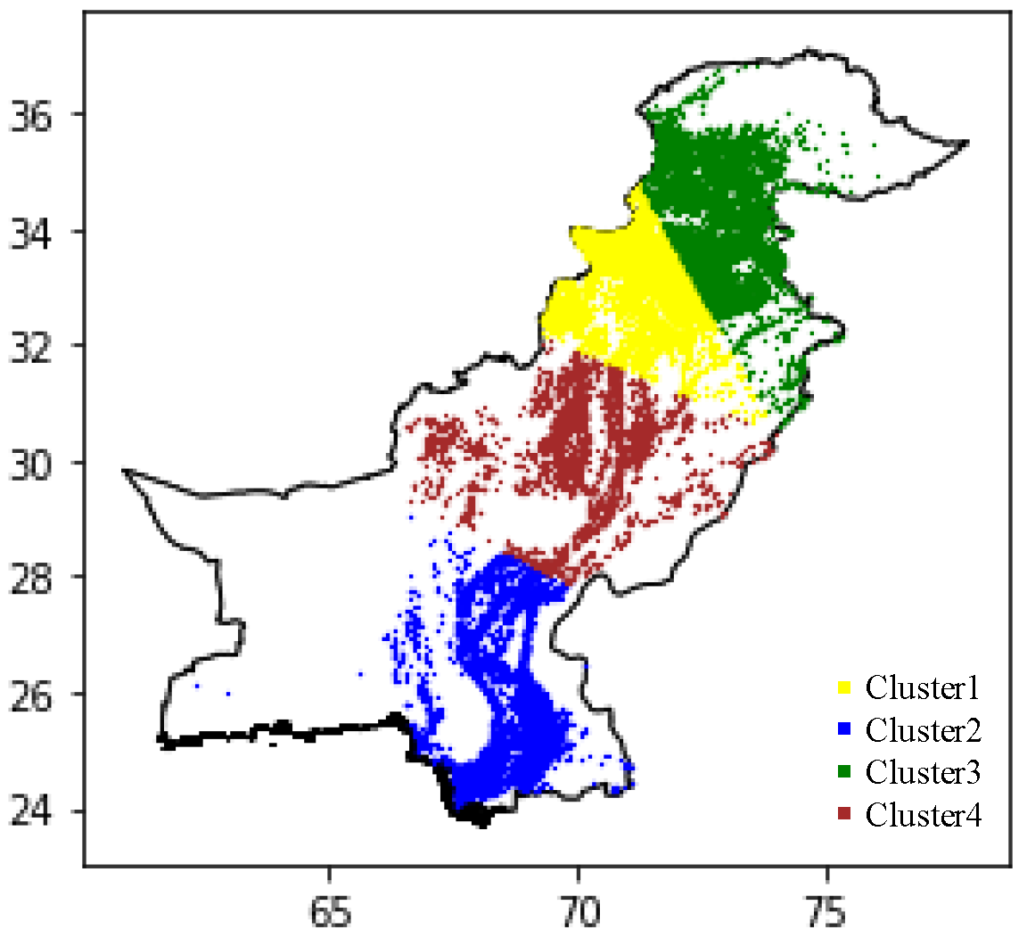
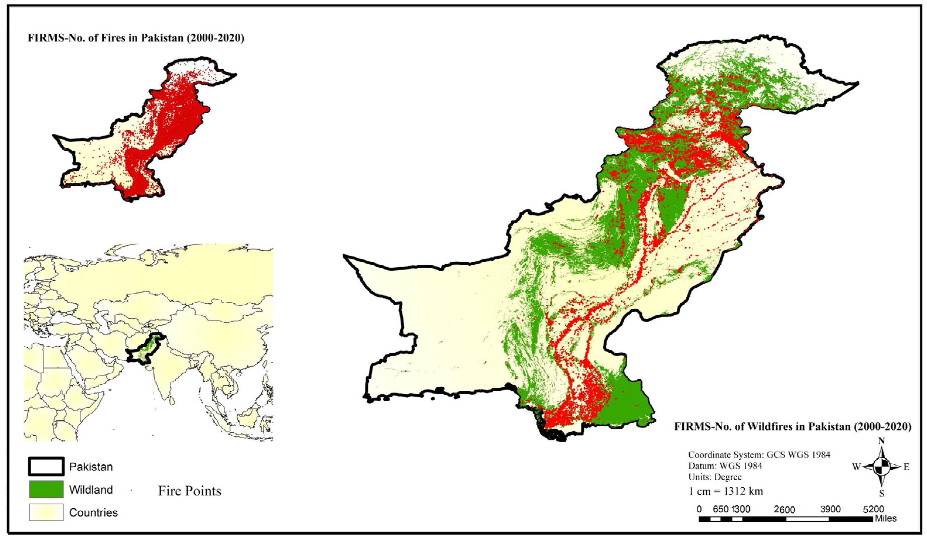
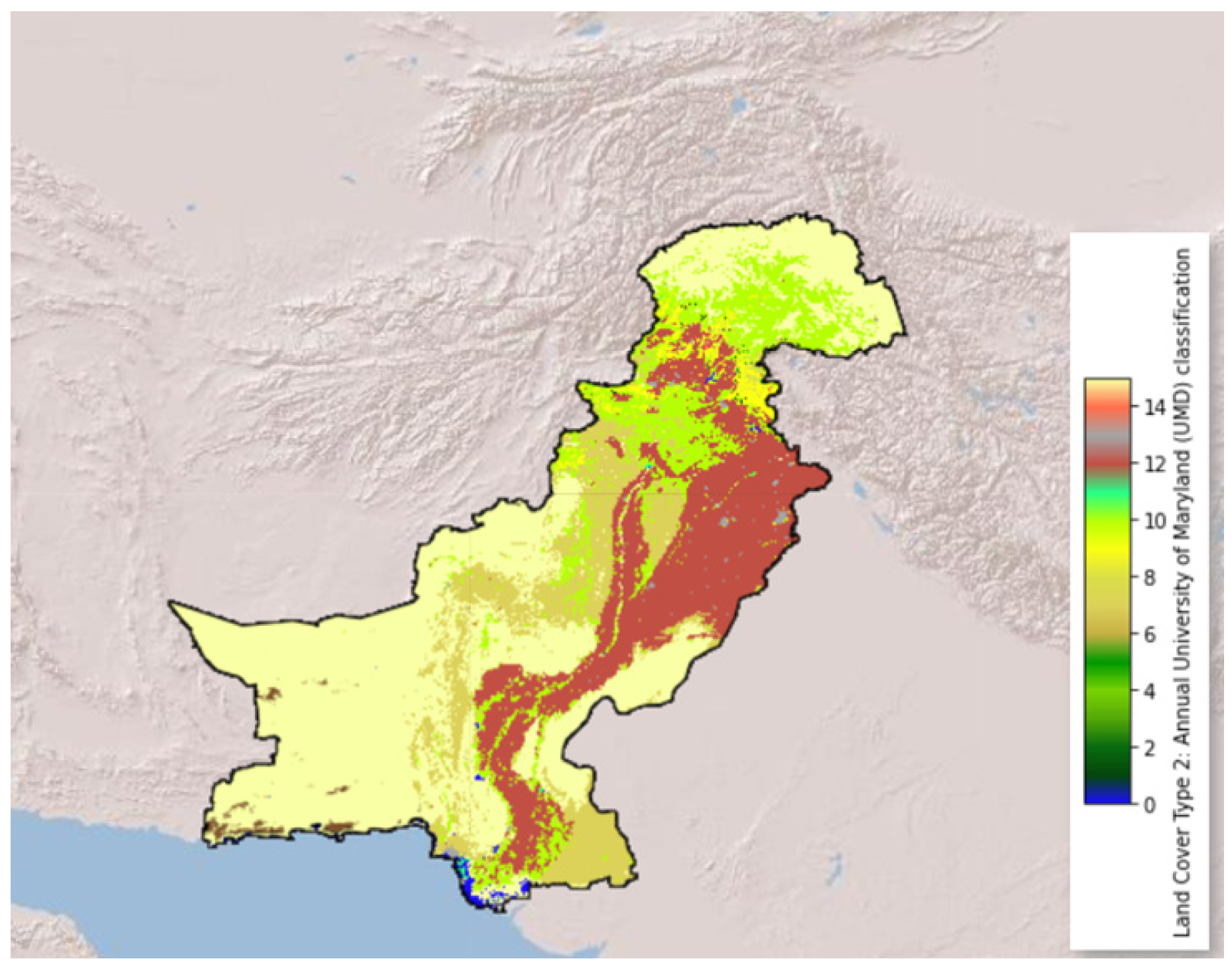
3. Study Area
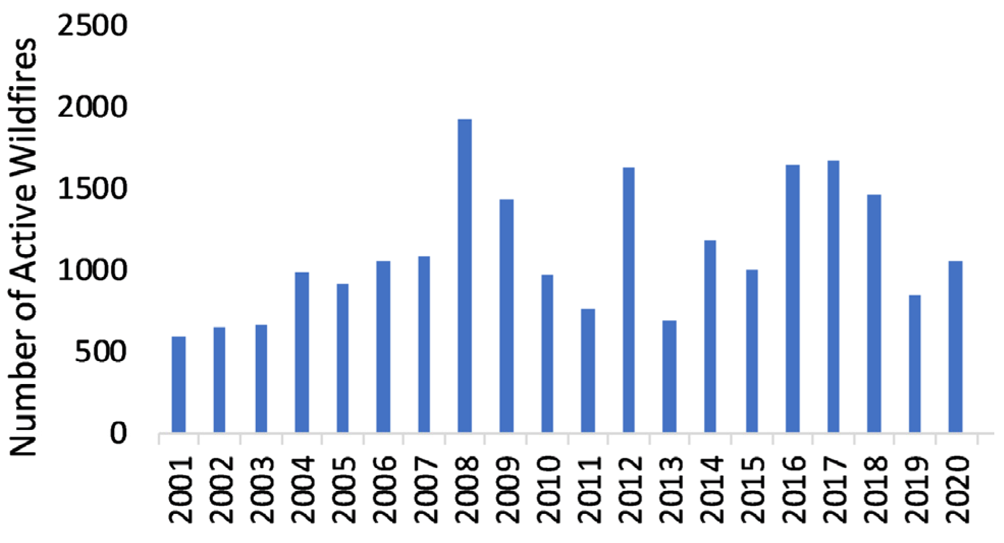
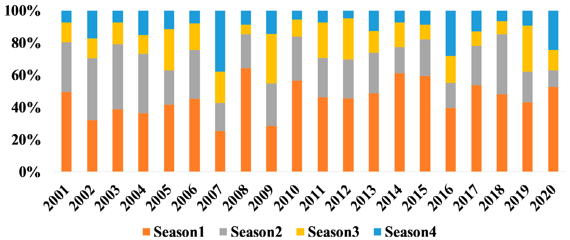
Exploratory Data Analysis: Historical Fire Events
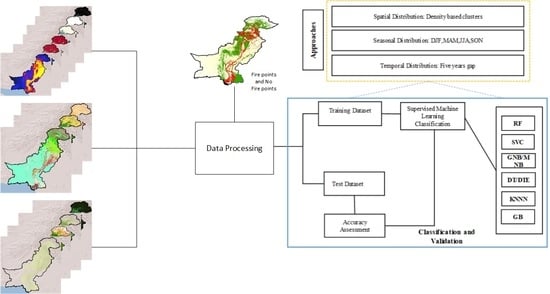
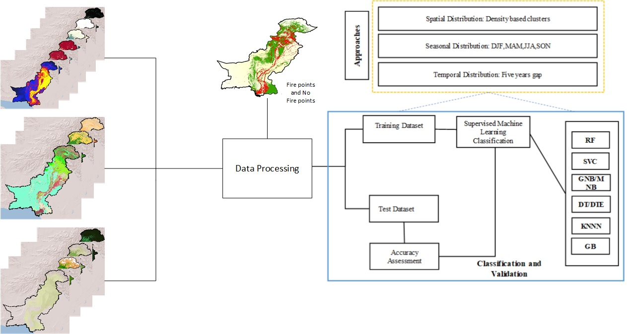
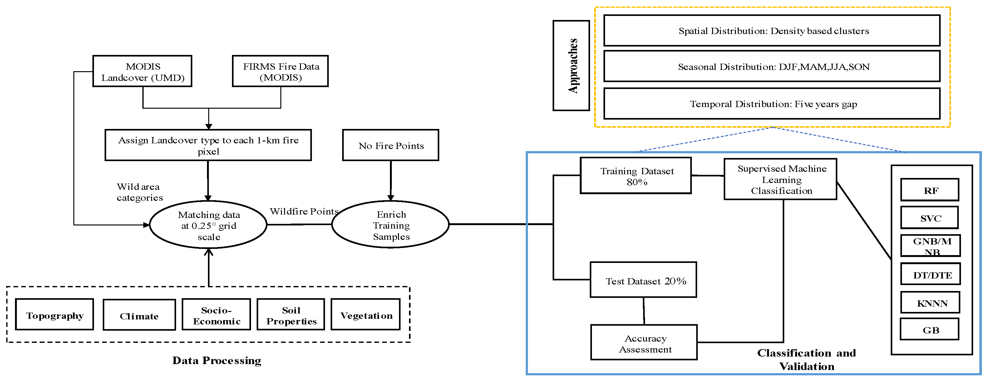
4. Methodology
4.1. Data Preparation and Preprocessing

| Category | Parameter | Source | Resolution | Unit | Time |
|---|---|---|---|---|---|
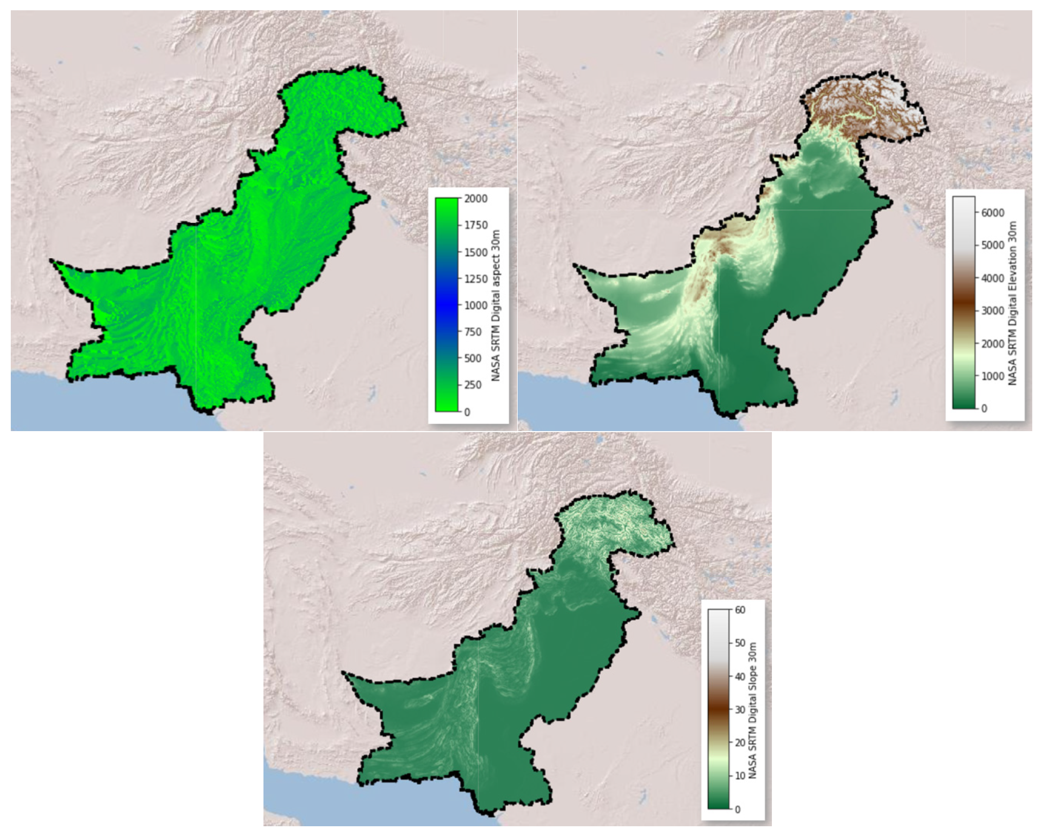
| Topography | Elevation | NASA SRTM Digital Elevation [79] | 30 m | m | 2000 |
| Slope | ° | ||||
| Aspect | |||||
| Hill shadow | |||||
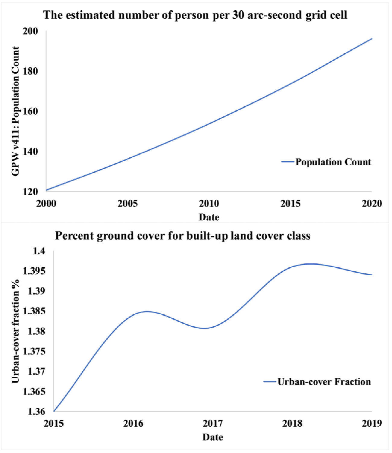
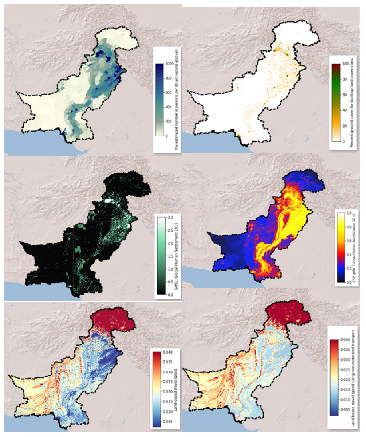
| Socioeconomic | Population | GPWv411: Population Count (Population Count) | 927.67 m | Count | 2000, 2005, 2010, 2015, and 2020 |
| Human modification | CSP gHM: Global Human Modification [80] | 1000 m | km2 | 2016 | |
| Travel speed | Oxford/MAP/friction_surface_2019 [81] | 927.67 m | min/m | 2019 | |
| Travel speed walk | |||||
| Settlement | GHSL: Global Human Settlement Layers [82] | 1000 m | classes | 1975–1990–2000–2014 (P2016) | |
| Urban cover | Copernicus Global Land Service (CGLS) [83] | % | 2015–2019 | ||
| Climate | Precipitation | Global Land Data Assimilation System [78] | 27,830 m | kg/m2/s | 2000–2021 |
| Transpiration | W/m2 | ||||
| Wind speed | m/s | ||||
| Soil temperature | k | ||||
| Humidity | kg/kg | ||||
| Heat flux | W/m2 | ||||
| Albedo | % | ||||
| Average surface skin temperature | k | ||||
| Soil moisture | kg/m2 | ||||
| Actual evapotranspiration | Terra Climate: Monthly Climate global [77] | 4638.3 m | mm | 1958–2020 | |
| Water deficit | |||||
| Precipitation accumulation | |||||
| Downward surface shortwave radiation | W/m2 | ||||
| Minimum temperature | °C | ||||
| Maximum temperature | |||||
| Vapor pressure | kPa | ||||
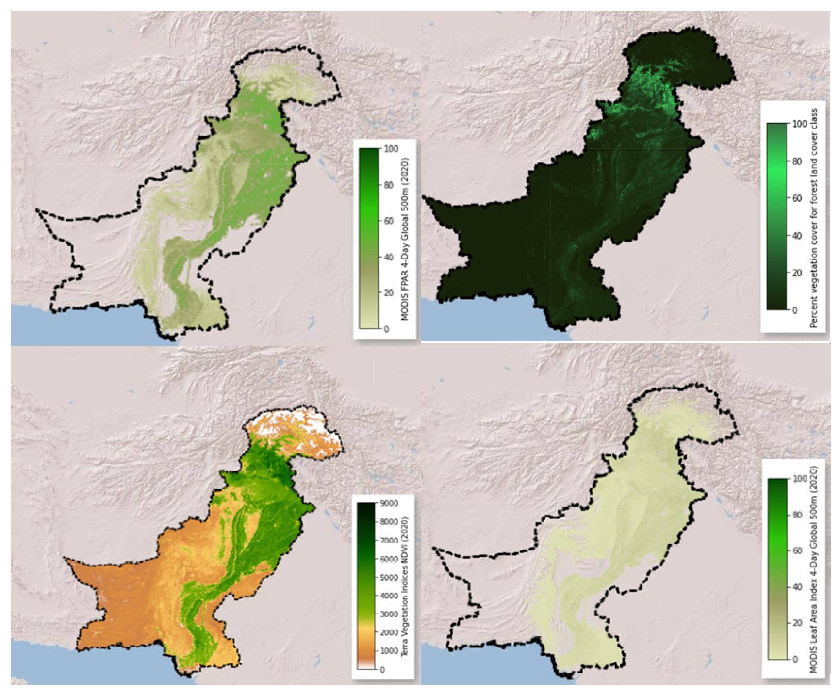
| Vegetation | Tree cover | Copernicus Global Land Service (CGLS) [82] | 1000 m | % | 2015–2019 |
| NDVI | MOD13A1.006 Terra Vegetation Indices (Terra Vegetation Indices) | 500 m | nm | 2000–2022 | |
| FPAR | MCD15A3H.006 MODIS Leaf Area Index/FPAR0m (Copernicus.) | ||||
| LAI | m2 | ||||
| Land cover | MCD12Q1.006 MODIS Land Cover Type (Modis Landcover) | classes | 2001–2020 | ||
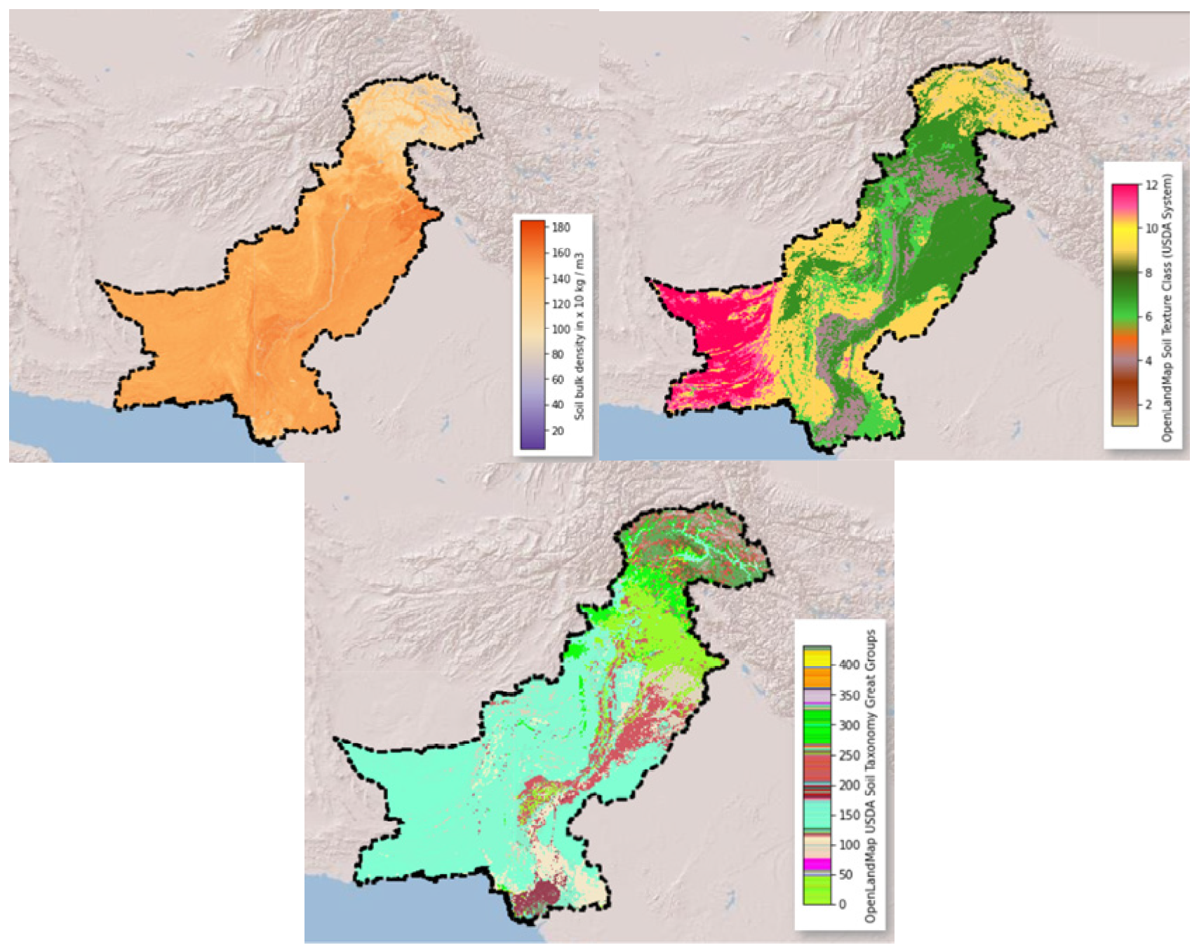
| Soil | Soil bulk density | OpenLandMap USDA [84] | 250 m | kg/m3 | 1950–2018 |
| Soil taxonomy | OpenLandMap USDA [85] | classes | 1950–2019 | ||
| Soil texture | OpenLandMap USDA [86] |
4.2. Classification
4.3. Validation and Evaluation Matrix
5. Results
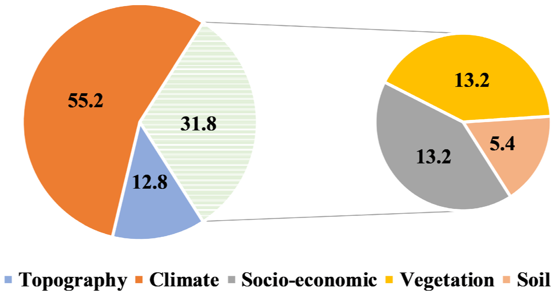
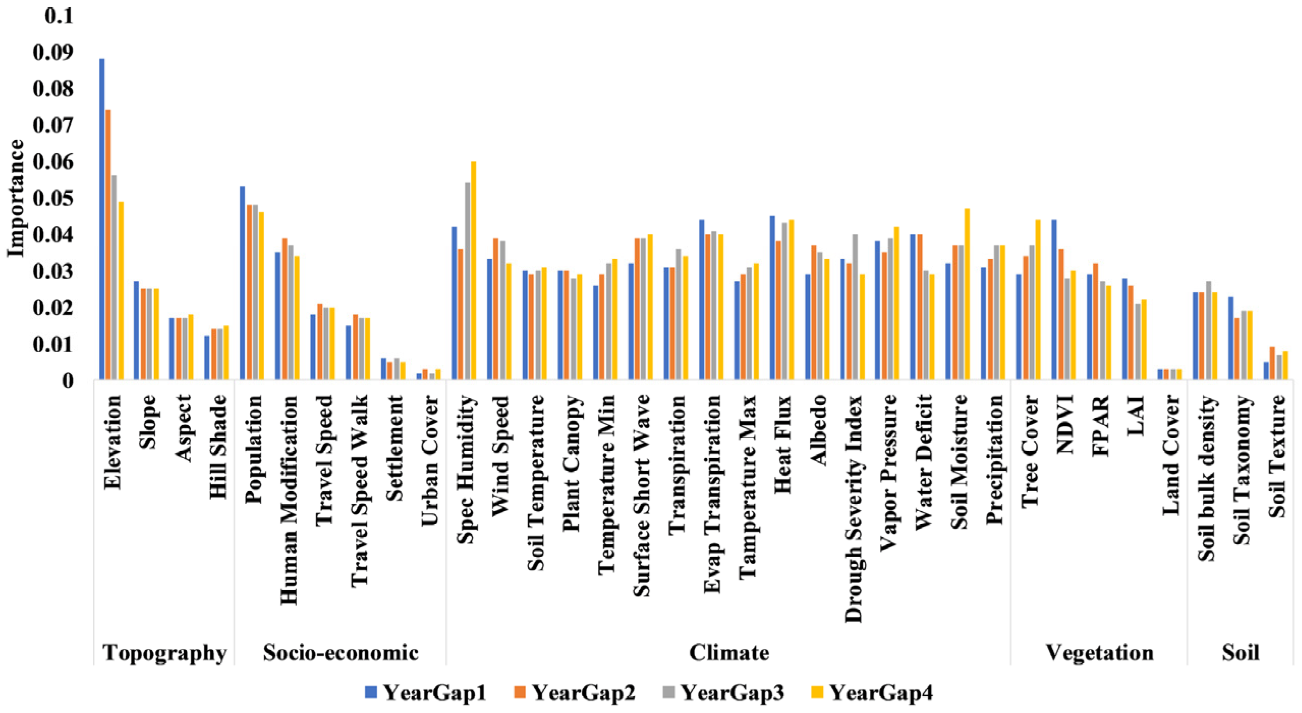
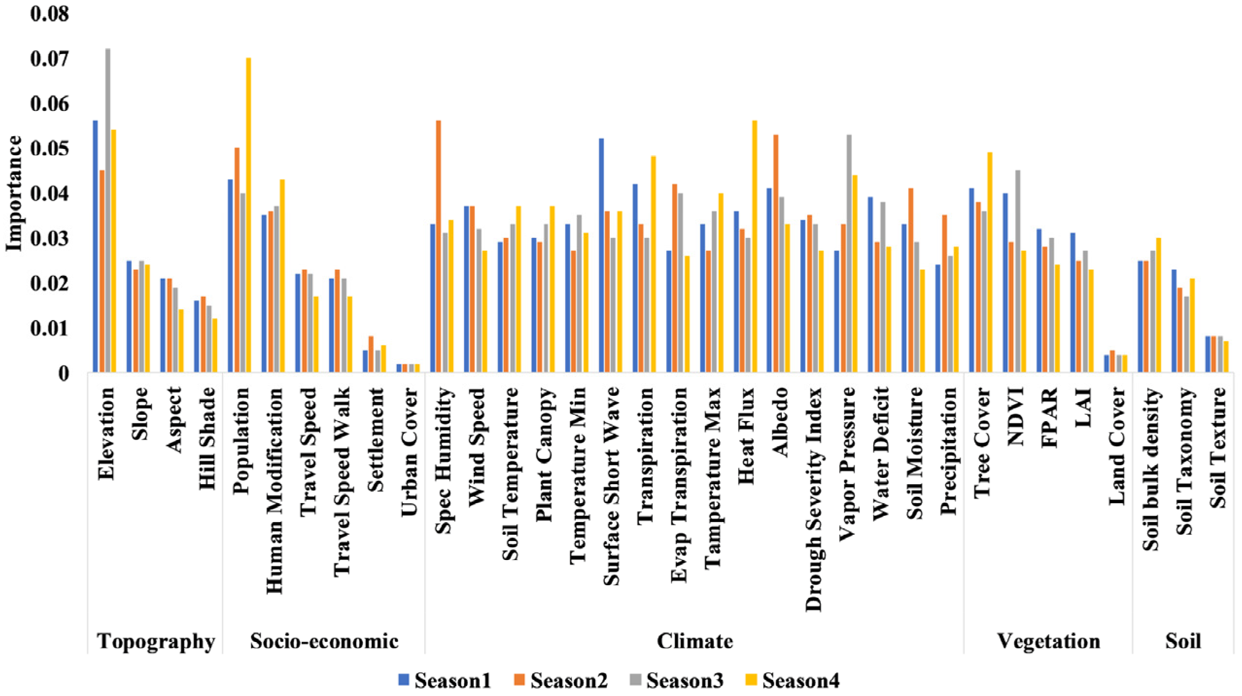
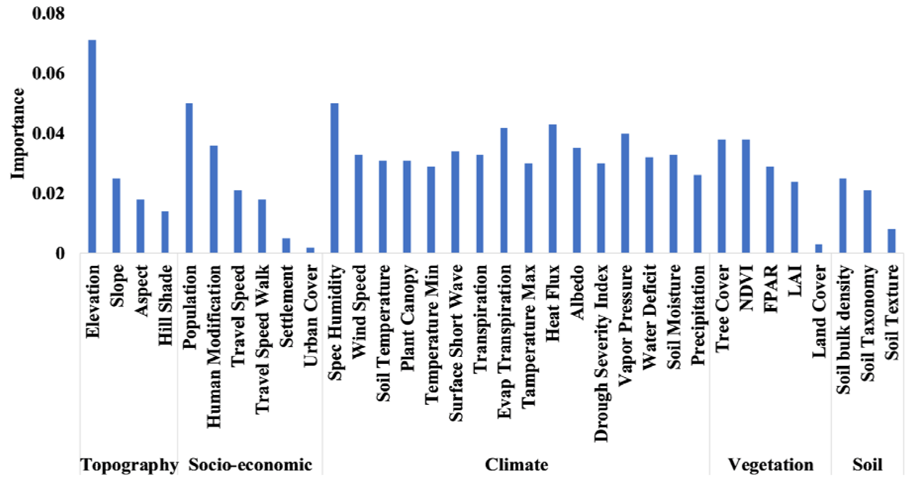
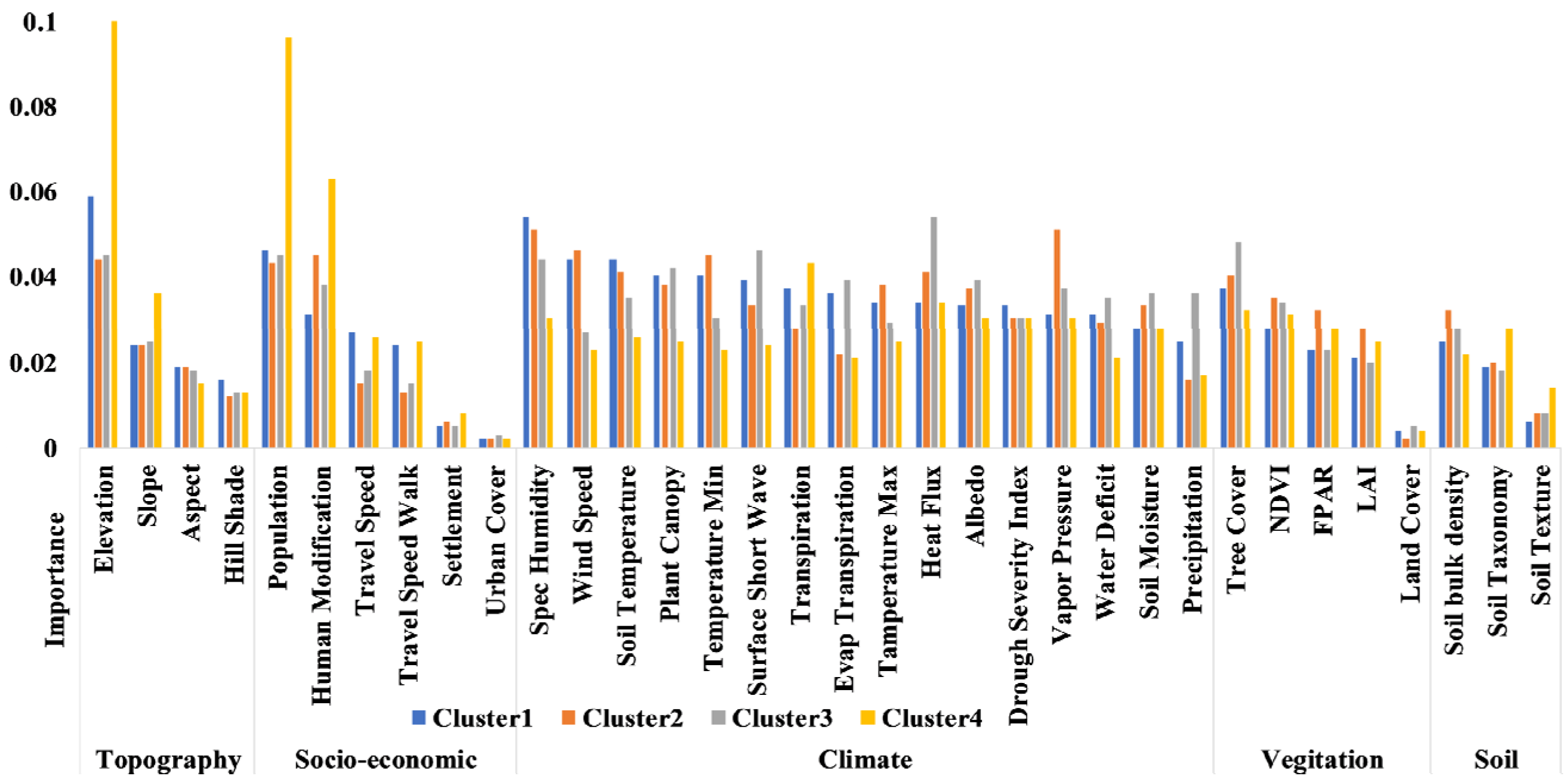
6. Feature Importance: Driving Factors
7. Discussion
8. Conclusions
9. Recommendations
- It is suggested that each subarea develop its own fire management plan. The management of wildland areas should be divided into subareas on the basis of density clusters, and the model should be trained using the appropriate datasets.
- The management of wildland areas should investigate fire behavior in different seasons, and a seasonal methodology plan for wildfire mitigation and management is unavoidable.
- One immediate application of our findings would be to transfer the population and essential facilities that are located in fire-prone regions, thus reducing the financial and public health losses.
- Our work can benefit the presently operational decision support systems for wildfire control in Pakistan in terms of data and model selection, as well as platform development.
- Using freely available global databases, all emerging countries can assess catastrophic risk and can utilize the information for better management.
10. Constraints and limitations
Author Contributions
Funding
Data Availability Statement
Conflicts of Interest
References
- Verde, J.; Zêzere, J. Assessment and validation of wildfire susceptibility and hazard in Portugal. Nat. Hazards Earth Syst. Sci. 2010, 10, 485–497. [Google Scholar] [CrossRef]
- FerreirA-leiTe, F.; Lourenço, L.; Bento-Gonçalves, A. Large forest fires in mainland Portugal, brief characterization. J. Mediterr. Geogr. 2013, 19, 53–65. [Google Scholar] [CrossRef]
- Tedim, F.; Remelgado, R.; Borges, C.; Carvalho, S.; Martins, J. Exploring the occurrence of mega-fires in Portugal. For. Ecol. Manag. 2013, 294, 86–96. [Google Scholar] [CrossRef]
- Neary, D.G.; Ryan, K.C.; DeBano, L.F. Wildland Fire in Ecosystems: Effects of Fire on Soils and Water, General Technical Report RMRSGTR-42-Volume 4; USDA, Forest Service, Rocky Mountain Research Station: Ogden, UT, USA, 2005; p. 250.
- Brown, J.K.; Smith, J.K. Wildland Fire in Ecosystems: Effects of Fire on Flora; US Department of Agriculture, Forest Service, Rocky Mountain Research Station: Ogden, UT, USA, 2000; p. 257.
- Xu, R.; Yu, P.; Abramson, M.J.; Johnston, F.H.; Samet, J.M.; Bell, M.L.; Haines, A.; Ebi, K.L.; Li, S.; Guo, Y. Wildfires, global climate change, and human health. N. Engl. J. Med. 2020, 383, 2173–2181. [Google Scholar] [CrossRef]
- Sandberg, D.V. Wildland Fire in Ecosystems: Effects of Fire on Air; US Department of Agriculture, Forest Service, Rocky Mountain Research Station: Ogden, UT, USA, 2003.
- Johnston, L.M.; Wang, X.; Erni, S.; Taylor, S.W.; McFayden, C.B.; Oliver, J.A.; Stockdale, C.; Christianson, A.; Boulanger, Y.; Gauthier, S. Wildland fire risk research in Canada. Environ. Rev. 2020, 28, 164–186. [Google Scholar] [CrossRef]
- Martell, D.L. Forest fire management. In Handbook of Operations Research in Natural Resources; Springer: Berlin/Heidelberg, Germany, 2007; pp. 489–509. [Google Scholar]
- González-Cabán, A. The economic dimension of wildland fires. In Vegetation Fires and Global Change—Challenges for Concerted International Action; Johann Georg, G., Ed.; A White Paper Directed to the United Nations and International Organizations; Kassel Publishing House: Kassel, Germany, 2013; pp. 229–237. [Google Scholar]
- Lavorel, S.; Flannigan, M.D.; Lambin, E.F.; Scholes, M.C. Vulnerability of land systems to fire: Interactions among humans, climate, the atmosphere, and ecosystems. Mitig. Adapt. Strateg. Glob. Chang. 2007, 12, 33–53. [Google Scholar] [CrossRef]
- Hantson, S.; Pueyo, S.; Chuvieco, E. Global fire size distribution is driven by human impact and climate. Glob. Ecol. Biogeogr. 2015, 24, 77–86. [Google Scholar] [CrossRef]
- Jolly, W.M.; Cochrane, M.A.; Freeborn, P.H.; Holden, Z.A.; Brown, T.J.; Williamson, G.J.; Bowman, D.M. Climate-induced variations in global wildfire danger from 1979 to 2013. Nat. Commun. 2015, 6, 7537. [Google Scholar] [CrossRef]
- Barbero, R.; Abatzoglou, J.T.; Pimont, F.; Ruffault, J.; Curt, T. Attributing increases in fire weather to anthropogenic climate change over France. Front. Earth Sci. 2020, 8, 104. [Google Scholar] [CrossRef]
- Oliveira, S.L.; Pereira, J.M.; Carreiras, J.M. Fire frequency analysis in Portugal (1975–2005), using Landsat-based burnt area maps. Int. J. Wildland Fire 2011, 21, 48–60. [Google Scholar] [CrossRef]
- Azevedo, J.; Pinto, M.; Perera, A. Forest Landscape Ecology and Global Change: What Are the Next Steps? Springer: Berlin/Heidelberg, Germany, 2014; pp. 249–260. [Google Scholar]
- Stacey, R.; Gibson, S.; Hedley, P. European Glossary for Wildfires and Forest Fires; European Union-INTERREG IVC: Cham, Switzerland, 2012. [Google Scholar]
- Álvarez-Díaz, M.; González-Gómez, M.; Otero-Giraldez, M.S. Detecting the socioeconomic driving forces of the fire catastrophe in NW Spain. Eur. J. For. Res. 2015, 134, 1087–1094. [Google Scholar] [CrossRef]
- Flannigan, M.D.; Wotton, B.M. Climate, weather, and area burned. In Forest Fires; Elsevier: Amsterdam, The Netherlands, 2001; pp. 351–373. [Google Scholar]
- Tymstra, C.; Jain, P.; Flannigan, M.D. Characterisation of initial fire weather conditions for large spring wildfires in Alberta, Canada. Int. J. Wildland Fire 2021, 30, 823–835. [Google Scholar] [CrossRef]
- Ganteaume, A.; Camia, A.; Jappiot, M.; San-Miguel-Ayanz, J.; Long-Fournel, M.; Lampin, C. A review of the main driving factors of forest fire ignition over Europe. Environ. Manag. 2013, 51, 651–662. [Google Scholar] [CrossRef] [PubMed] [Green Version]
- Keeley, J.E.; Syphard, A.D. Climate change and future fire regimes: Examples from California. Geosciences 2016, 6, 37. [Google Scholar] [CrossRef] [Green Version]
- Nunes, A.; Lourenço, L.; Meira, A.C. Exploring spatial patterns and drivers of forest fires in Portugal (1980–2014). Sci. Total Environ. 2016, 573, 1190–1202. [Google Scholar] [CrossRef] [PubMed]
- Cao, X.; Cui, X.; Yue, M.; Chen, J.; Tanikawa, H.; Ye, Y. Evaluation of wildfire propagation susceptibility in grasslands using burned areas and multivariate logistic regression. Int. J. Remote Sens. 2013, 34, 6679–6700. [Google Scholar] [CrossRef]
- Holsinger, L.; Parks, S.A.; Miller, C. Weather, fuels, and topography impede wildland fire spread in western US landscapes. For. Ecol. Manag. 2016, 380, 59–69. [Google Scholar] [CrossRef]
- Calviño-Cancela, M.; Chas-Amil, M.L.; García-Martínez, E.D.; Touza, J. Wildfire risk associated with different vegetation types within and outside wildland-urban interfaces. For. Ecol. Manag. 2016, 372, 1–9. [Google Scholar] [CrossRef] [Green Version]
- Barreiro, J.B.; HerMosillA, T. Socio-geographic analysis of the causes of the 2006’s wildfires in Galicia (Spain). For. Syst. 2013, 22, 497–509. [Google Scholar] [CrossRef] [Green Version]
- Keeley, J.E.; Syphard, A.D. Historical patterns of wildfire ignition sources in California ecosystems. Int. J. Wildland Fire 2018, 27, 781–799. [Google Scholar] [CrossRef] [Green Version]
- Rodrigues, M.; Jiménez, A.; de la Riva, J. Analysis of recent spatial–temporal evolution of human driving factors of wildfires in Spain. Nat. Hazards 2016, 84, 2049–2070. [Google Scholar] [CrossRef] [Green Version]
- Vilar del Hoyo, L.; Martín Isabel, M.P.; Martínez Vega, F.J. Logistic regression models for human-caused wildfire risk estimation: Analysing the effect of the spatial accuracy in fire occurrence data. Eur. J. For. Res. 2011, 130, 983–996. [Google Scholar] [CrossRef]
- Tien Bui, D.; Le, K.-T.T.; Nguyen, V.C.; Le, H.D.; Revhaug, I. Tropical forest fire susceptibility mapping at the Cat Ba National Park Area, Hai Phong City, Vietnam, using GIS-based kernel logistic regression. Remote Sens. 2016, 8, 347. [Google Scholar] [CrossRef] [Green Version]
- Ghorbanzadeh, O.; Valizadeh Kamran, K.; Blaschke, T.; Aryal, J.; Naboureh, A.; Einali, J.; Bian, J. Spatial prediction of wildfire susceptibility using field survey gps data and machine learning approaches. Fire 2019, 2, 43. [Google Scholar] [CrossRef] [Green Version]
- Tyagi, A.K. Machine learning with big data (March 20, 2019). In Proceedings of the International Conference on Sustainable Computing in Science, Technology and Management (SUSCOM), Amity University Rajasthan, Jaipur, India, 26–28 February 2019. [Google Scholar]
- Iqbal, M.; Sameem, M.S.I.; Naqvi, N.; Kanwal, S.; Ye, Z. A deep learning approach for face recognition based on angularly discriminative features. Pattern Recognit. Lett. 2019, 128, 414–419. [Google Scholar] [CrossRef]
- Gould, J.S.; McCaw, W.; Cheney, N.; Ellis, P.F.; Knight, I.; Sullivan, A.L. Project Vesta: Fire in Dry Eucalypt Forest: Fuel Structure, Fuel Dynamics and Fire Behaviour; Csiro Publishing: Clayton, Australia, 2008. [Google Scholar]
- Cruz, M.; McCaw, L.; Anderson, W.; Gould, J. Fire behaviour modelling in semi-arid mallee-heath shrublands of southern Australia. Environ. Model. Softw. 2013, 40, 21–34. [Google Scholar] [CrossRef]
- Phelps, N.; Woolford, D.G. Comparing calibrated statistical and machine learning methods for wildland fire occurrence prediction: A case study of human-caused fires in Lac La Biche, Alberta, Canada. Int. J. Wildland Fire 2021, 30, 850–870. [Google Scholar] [CrossRef]
- Khalid, N.; Ahmad, S.; Erum, S.; Butt, A. Monitoring forest cover change of Margalla Hills over a period of two decades (1992–2011): A spatiotemporal perspective. J. Ecosyst. Ecography 2015, 6, 174–181. [Google Scholar] [CrossRef]
- chAs-AMil, M.L.; TouzA, J.; García-Martínez, E. Forest fires in the wildland–urban interface: A spatial analysis of forest fragmentation and human impacts. Appl. Geogr. 2013, 43, 127–137. [Google Scholar] [CrossRef]
- Bowman, D.M.; Balch, J.; Artaxo, P.; Bond, W.J.; Cochrane, M.A.; D’antonio, C.M.; DeFries, R.; Johnston, F.H.; Keeley, J.E.; Krawchuk, M.A. The human dimension of fire regimes on Earth. J. Biogeogr. 2011, 38, 2223–2236. [Google Scholar] [CrossRef] [Green Version]
- Syphard, A.D.; Radeloff, V.C.; Keeley, J.E.; Hawbaker, T.J.; Clayton, M.K.; Stewart, S.I.; Hammer, R.B. Human influence on California fire regimes. Ecol. Appl. 2007, 17, 1388–1402. [Google Scholar] [CrossRef] [PubMed]
- Narayanaraj, G.; Wimberly, M.C. Influences of forest roads on the spatial patterns of human- and lightning-caused wildfire ignitions. Appl. Geogr. 2012, 32, 878–888. [Google Scholar] [CrossRef]
- Roy, D.; Wulder, M.; Loveland, T. Landsat-8: Science and product vision for terrestrial global change research. Remote Sens. Environ. 2014, 15, 154–172. [Google Scholar] [CrossRef] [Green Version]
- Plucinski, M.; McCaw, W.; Gould, J.; Wotton, B. Predicting the number of daily human-caused bushfires to assist suppression planning in south-west Western Australia. Int. J. Wildland Fire 2014, 23, 520–531. [Google Scholar] [CrossRef]
- Costafreda-Aumedes, S.; Comas, C.; Vega-Garcia, C. Human-caused fire occurrence modelling in perspective: A review. Int. J. Wildland Fire 2017, 26, 983–998. [Google Scholar] [CrossRef]
- Taylor, S.W.; Woolford, D.G.; Dean, C.; Martell, D.L. Wildfire prediction to inform fire management: Statistical science challenges. Stat. Sci. 2013, 28, 586–615. [Google Scholar] [CrossRef] [Green Version]
- Nadeem, K.; Taylor, S.; Woolford, D.G.; Dean, C. Mesoscale spatiotemporal predictive models of daily human-and lightning-caused wildland fire occurrence in British Columbia. Int. J. Wildland Fire 2019, 29, 11–27. [Google Scholar] [CrossRef]
- Woolford, D.G.; Martell, D.L.; McFayden, C.B.; Evens, J.; Stacey, A.; Wotton, B.M.; Boychuk, D. The development and implementation of a human-caused wildland fire occurrence prediction system for the province of Ontario, Canada. Can. J. For. Res. 2021, 51, 303–325. [Google Scholar] [CrossRef]
- Ghorbanzadeh, O.; Blaschke, T.; Gholamnia, K.; Aryal, J. Forest fire susceptibility and risk mapping using social/infrastructural vulnerability and environmental variables. Fire 2019, 2, 50. [Google Scholar] [CrossRef] [Green Version]
- Gigović, L.; Pourghasemi, H.R.; Drobnjak, S.; Bai, S. Testing a new ensemble model based on SVM and random forest in forest fire susceptibility assessment and its mapping in Serbia’s Tara National Park. Forests 2019, 10, 408. [Google Scholar] [CrossRef] [Green Version]
- Tehrany, M.S.; Jones, S.; Shabani, F.; Martínez-Álvarez, F.; Tien Bui, D. A novel ensemble modeling approach for the spatial prediction of tropical forest fire susceptibility using LogitBoost machine learning classifier and multi-source geospatial data. Theor. Appl. Climatol. 2019, 137, 637–653. [Google Scholar] [CrossRef]
- Mohajane, M.; Costache, R.; Karimi, F.; Pham, Q.B.; Essahlaoui, A.; Nguyen, H.; Laneve, G.; Oudija, F. Application of remote sensing and machine learning algorithms for forest fire mapping in a Mediterranean area. Ecol. Indic. 2021, 129, 107869. [Google Scholar] [CrossRef]
- Gholamnia, K.; Gudiyangada Nachappa, T.; Ghorbanzadeh, O.; Blaschke, T. Comparisons of diverse machine learning approaches for wildfire susceptibility mapping. Symmetry 2020, 12, 604. [Google Scholar] [CrossRef] [Green Version]
- Wang, S.S.C.; Qian, Y.; Leung, L.R.; Zhang, Y. Identifying key drivers of wildfires in the contiguous US using machine learning and game theory interpretation. Earth Future 2021, 9, e2020EF001910. [Google Scholar] [CrossRef] [PubMed]
- Calviño-Cancela, M.; Chas-Amil, M.L.; García-Martínez, E.D.; Touza, J. Interacting effects of topography, vegetation, human activities and wildland-urban interfaces on wildfire ignition risk. For. Ecol. Manag. 2017, 397, 10–17. [Google Scholar] [CrossRef] [Green Version]
- San-Miguel-Ayanz, J.; Moreno, J.M.; Camia, A. Analysis of large fires in European Mediterranean landscapes: Lessons learned and perspectives. For. Ecol. Manag. 2013, 294, 11–22. [Google Scholar] [CrossRef]
- Xi, D.D.; Taylor, S.W.; Woolford, D.G.; Dean, C. Statistical models of key components of wildfire risk. Annu. Rev. Stat. Its Appl. 2019, 6, 197–222. [Google Scholar] [CrossRef]
- Ghorbanzadeh, O.; Meena, S.R.; Abadi, H.S.S.; Piralilou, S.T.; Zhiyong, L.; Blaschke, T. Landslide Mapping Using Two Main Deep-Learning Convolution Neural Network Streams Combined by the Dempster–Shafer Model. IEEE J. Sel. Top. Appl. Earth Obs. Remote Sens. 2020, 14, 452–463. [Google Scholar] [CrossRef]
- Neale, T.; Vergani, M.; Begg, C.; Kilinc, M.; Wouters, M.; Harris, S. ‘Any prediction is better than none’? A study of the perceptions of fire behaviour analysis users in Australia. Int. J. Wildland Fire 2021, 30, 946–953. [Google Scholar] [CrossRef]
- Wotton, B.M. Interpreting and using outputs from the Canadian Forest Fire Danger Rating System in research applications. Environ. Ecol. Stat. 2009, 16, 107–131. [Google Scholar] [CrossRef]
- Turner, R. Point patterns of forest fire locations. Environ. Ecol. Stat. 2009, 16, 197–223. [Google Scholar] [CrossRef]
- Kattel, D.B.; Yao, T.; Ullah, K.; Rana, A.S. Seasonal near-surface air temperature dependence on elevation and geographical coordinates for Pakistan. Theor. Appl. Climatol. 2019, 138, 1591–1613. [Google Scholar] [CrossRef]
- Begum, B.A.; Biswas, S.K.; Pandit, G.G.; Saradhi, I.V.; Waheed, S.; Siddique, N.; Seneviratne, M.S.; Cohen, D.D.; Markwitz, A.; Hopke, P.K. Long–range transport of soil dust and smoke pollution in the South Asian region. Atmos. Pollut. Res. 2011, 2, 151–157. [Google Scholar] [CrossRef] [Green Version]
- MODIS/Aqua + Terra Thermal Anomalies/Fire Locations 1 km FIRMS V006 NRT (Vector Data). Available online: https://data.amerigeoss.org/nl/dataset/modis-aqua-terra-thermal-anomalies-fire-locations-1km-firms-v006-nrt-vector-data (accessed on 15 March 2022).
- Hanson, M.; Defries, R.; Townshend, J.; Sohlberg, R. Global land cover classification at 1 km spatial resolution using a classifcation tree approach. Int. J. Remote Sens 2000, 21, 1331–1364. [Google Scholar] [CrossRef]
- Meira Castro, A.C.; Nunes, A.; Sousa, A.; Lourenço, L. Mapping the causes of forest fires in portugal by clustering analysis. Geosciences 2020, 10, 53. [Google Scholar] [CrossRef] [Green Version]
- Nolan, R.H.; Boer, M.M.; Collins, L.; Resco de Dios, V.; Clarke, H.G.; Jenkins, M.; Kenny, B.; Bradstock, R.A. Causes and consequences of eastern Australia’s 2019-20 season of mega-fires. Glob. Chang. Biol. 2020, 26, 1039–1041. [Google Scholar] [CrossRef] [Green Version]
- Edwards, R.B.; Naylor, R.L.; Higgins, M.M.; Falcon, W.P. Causes of Indonesia’s forest fires. World Dev. 2020, 127, 104717. [Google Scholar] [CrossRef]
- Tien Bui, D.; Tuan, T.A.; Hoang, N.-D.; Thanh, N.Q.; Nguyen, D.B.; Van Liem, N.; Pradhan, B. Spatial prediction of rainfall-induced landslides for the Lao Cai area (Vietnam) using a hybrid intelligent approach of least squares support vector machines inference model and artificial bee colony optimization. Landslides 2017, 14, 447–458. [Google Scholar] [CrossRef]
- Van Wagner, C.; Forest, P. Development and Structure of the Canadian Forest Fireweather Index System. Can. For. Serv. For. Tech. Rep. 1987. Available online: http://citeseerx.ist.psu.edu/viewdoc/summary?doi=10.1.1.460.3231 (accessed on 15 March 2022).
- Lawson, B.D.; Armitage, O. Weather Guide for the Canadian Forest Fire Danger Rating System; Northern Forestry Centre: Edmonton, AB, Canada, 2008. [Google Scholar]
- Mölders, N. Suitability of the Weather Research and Forecasting (WRF) model to predict the June 2005 fire weather for Interior Alaska. Weather Forecast. 2008, 23, 953–973. [Google Scholar] [CrossRef]
- Horel, J.D.; Ziel, R.; Galli, C.; Pechmann, J.; Dong, X. An evaluation of fire danger and behaviour indices in the Great Lakes Region calculated from station and gridded weather information. Int. J. Wildland Fire 2014, 23, 202–214. [Google Scholar] [CrossRef]
- De Jong, M.C.; Wooster, M.J.; Kitchen, K.; Manley, C.; Gazzard, R.; McCall, F.F. Calibration and evaluation of the Canadian Forest Fire Weather Index (FWI) System for improved wildland fire danger rating in the United Kingdom. Nat. Hazards Earth Syst. Sci. 2016, 16, 1217–1237. [Google Scholar] [CrossRef] [Green Version]
- Romero, R.; Mestre, A.; Botey, R. A New Calibration for Fire Weather Index in Spain (AEMET); Imprensa da Universidade de Coimbra: Coimbra, Portugal, 2014; Available online: http://hdl.handle.net/10316.2/34013 (accessed on 15 March 2022).
- Tian, X.-R.; Zhao, F.-J.; Shu, L.-F.; Wang, M.-Y. Changes in forest fire danger for south-western China in the 21st century. Int. J. Wildland Fire 2014, 23, 185–195. [Google Scholar] [CrossRef]
- Abatzoglou, J.T.; Dobrowski, S.Z.; Parks, S.A.; Hegewisch, K.C. TerraClimate, a high-resolution global dataset of monthly climate and climatic water balance from 1958–2015. Sci. Data 2018, 5, 170191. [Google Scholar] [CrossRef] [PubMed] [Green Version]
- Rodell, M.; Houser, P.; Jambor, U.; Gottschalck, J.; Mitchell, K.; Meng, C.-J.; Arsenault, K.; Cosgrove, B.; Radakovich, J.; Bosilovich, M. The global land data assimilation system. Bull. Am. Meteorol. Soc. 2004, 85, 381–394. [Google Scholar] [CrossRef] [Green Version]
- Farr, T.G.; Rosen, P.A.; Caro, E.; Crippen, R.; Duren, R.; Hensley, S.; Kobrick, M.; Paller, M.; Rodriguez, E.; Roth, L.; et al. The Shuttle Radar Topography Mission. Rev. Geophys. 2007, 45, RG2004. [Google Scholar] [CrossRef] [Green Version]
- Kennedy, C.M.; Oakleaf, J.R.; Theobald, D.M.; Baruch-Mordo, S.; Kiesecker, J. Managing the middle: A shift in conservation priorities based on the global human modification gradient. Glob. Chang. Biol. 2019, 25, 811–826. [Google Scholar] [CrossRef]
- Weiss, D.; Nelson, A.; Vargas-Ruiz, C.; Gligorić, K.; Bavadekar, S.; Gabrilovich, E.; Bertozzi-Villa, A.; Rozier, J.; Gibson, H.; Shekel, T. Global maps of travel time to healthcare facilities. Nat. Med. 2020, 26, 1835–1838. [Google Scholar] [CrossRef]
- Buchhorn, M.; Lesiv, M.; Tsendbazar, N.-E.; Herold, M.; Bertels, L.; Smets, B. Copernicus global land cover layers—Collection 2. Remote Sens. 2020, 12, 1044. [Google Scholar] [CrossRef] [Green Version]
- Pesaresi, M.; Huadong, G.; Blaes, X.; Ehrlich, D.; Ferri, S.; Gueguen, L.; Halkia, M.; Kauffmann, M.; Kemper, T.; Linlin Lu, M.-H.; et al. A global human settlement layer from optical HR/VHR RS data: Concept and first results. IEEE J. Sel. Top. Appl. Earth Obs. Remote Sens. 2013, 6, 2102–2131. [Google Scholar] [CrossRef]
- Hengl, T. Soil Bulk Density (Fine Earth) 10 × kg/m-Cubic at 6 Standard Depths (0, 10, 30, 60, 100 and 200 cm) at 250 m Resolution; Zenodo: Geneva, Switzerland, 2018. [Google Scholar]
- Hengl, T.; Nauman, T. Predicted USDA SOIL Great Groups at 250 m (Probabilities), v0.2 ed.; Zenodo: Geneva, Switzerland, 2018. [Google Scholar]
- Hengl, T. Soil Texture Classes (USDA System) for 6 Soil Depths (0, 10, 30, 60, 100 and 200 cm) at 250 m, v0.2 ed.; Zenodo: Geneva, Switzerland, 2018. [Google Scholar]
- Breiman, L. Bagging predictors. Mach. Learn. 1996, 24, 123–140. [Google Scholar] [CrossRef] [Green Version]
- Naumovich, V.V.; Vlamimir, V. Statistical Learning Theory; Wiley: New York, NY, USA, 1998. [Google Scholar]
- Cherkassky, V.; Mulier, F.M. Learning from Data: Concepts, Theory, and Methods; John Wiley & Sons: Hoboken, NJ, USA, 2007. [Google Scholar]
- Theodoridis, S. Machine Learning: A Bayesian and Optimization Perspective; Academic Press: Cambridge, MA, USA, 2015. [Google Scholar]
- Altman, N.S. An introduction to kernel and nearest-neighbor nonparametric regression. Am. Stat. 1992, 46, 175–185. [Google Scholar]
- Chen, T.; Guestrin, C. XGBoost: A Scalable Tree Boosting System. In Proceedings of the 22nd ACM SIGKDD International Conference on Knowledge Discovery and Data Mining, San Francisco, CA, USA, 13–17 August 2016; pp. 785–794. [Google Scholar]
- Metz, C. Basic principles of ROC analysis. [ROC = receiver operating characteristic, a factor used in decision making regarding the optimization of diagnostic techniques]. Semin. Nucl. Med. 1978, 8, 283–298. [Google Scholar] [CrossRef]
- Choubin, B.; Abdolshahnejad, M.; Moradi, E.; Querol, X.; Mosavi, A.; Shamshirband, S.; Ghamisi, P. Spatial hazard assessment of the PM10 using machine learning models in Barcelona, Spain. Sci. Total Environ. 2020, 701, 134474. [Google Scholar] [CrossRef] [PubMed]
- Donoho, D. 50 Years of Data Science. J. Comput. Graph. Stat. 2017, 26, 745–766. [Google Scholar] [CrossRef]
- Li, Y.; Wu, H. A clustering method based on K-means algorithm. Phys. Procedia 2012, 25, 1104–1109. [Google Scholar] [CrossRef] [Green Version]
- Van Beusekom, A.E.; Gould, W.A.; Monmany, A.; Khalyani, A.H.; Quiñones, M.; Fain, S.J.; Andrade-Núñez, M.J.; González, G. Fire weather and likelihood: Characterizing climate space for fire occurrence and extent in Puerto Rico. Clim. Chang. 2018, 146, 117–131. [Google Scholar] [CrossRef]
- Stojanova, D.; Kobler, A.; Ogrinc, P.; Ženko, B.; Džeroski, S. Estimating the risk of fire outbreaks in the natural environment. Data Min. Knowl. Discov. 2012, 24, 411–442. [Google Scholar] [CrossRef]


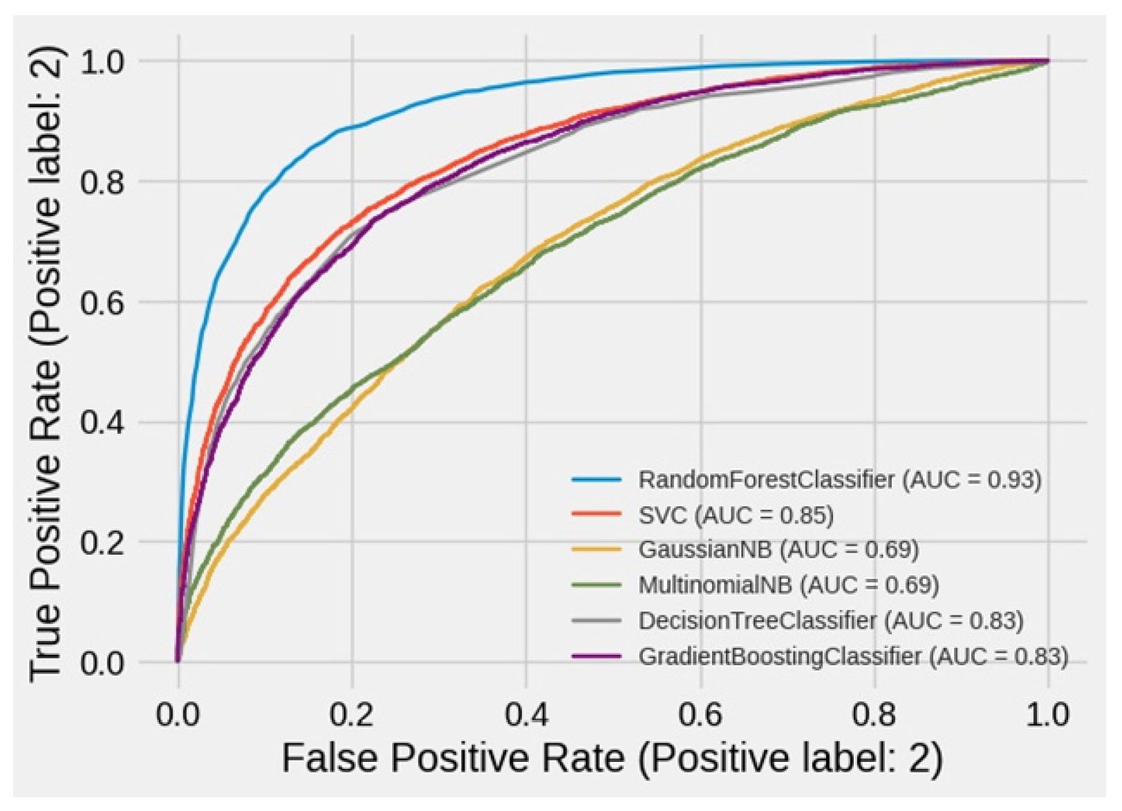
| Classifier | Accuracy Score | AUC Score | Precision Score |
|---|---|---|---|
| RF | 85.19 | 84.72 | 83.82 |
| SVC | 76.59 | 75.93 | 73.66 |
| GNB | 59.47 | 61.62 | 52 |
| MNB | 57.66 | 51.21 | 62.19 |
| DT | 75.12 | 75.11 | 69.62 |
| DTE | 74.06 | 74.33 | 67.64 |
| KNN | 75.89 | 75.81 | 70.7 |
| GB | 75.43 | 74.65 | 72.63 |
| Classifier | Accuracy Score | AUC Score | Precision Score |
|---|---|---|---|
| RF | 85.38 | 84.93 | 83.98 |
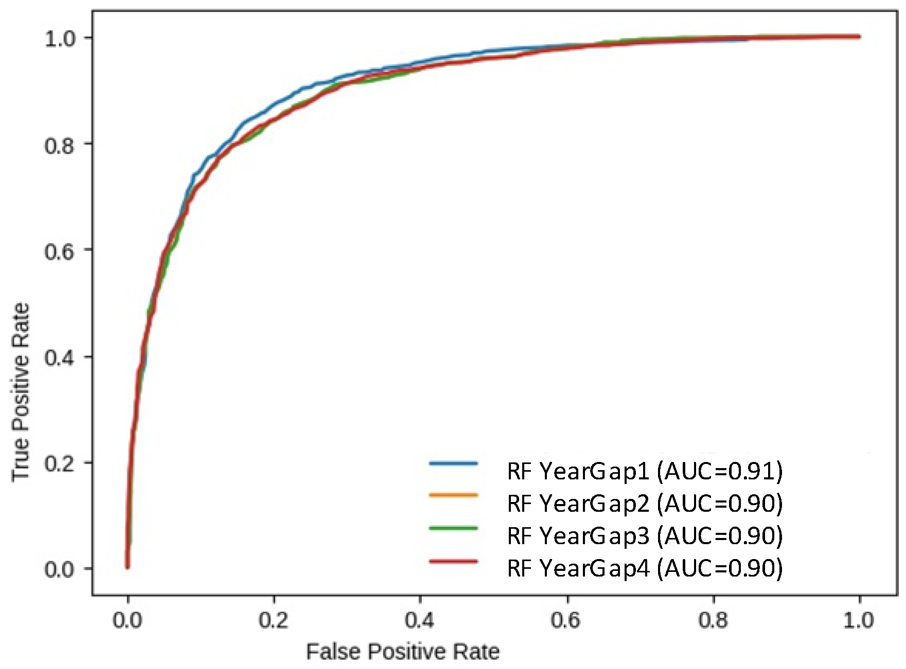
| Classifier | Accuracy Score | AUC Score | Precision Score |
|---|---|---|---|
| RFY1 | 84.74 | 82.2 | 82.6 |
| RFY2 | 82.24 | 82.07 | 81.92 |
| RFY3 | 83.95 | 83.63 | 84.46 |
| RFY4 | 82.39 | 82.31 | 81.16 |
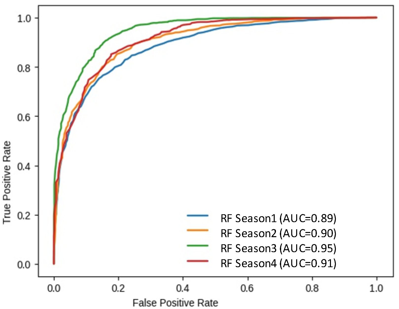
| Classifier | Accuracy Score | AUC Score | Precision Score |
|---|---|---|---|
| RFS1 | 81.47 | 79.35 | 81.58 |
| RFS2 | 82.61 | 81.92 | 82.25 |
| RFS3 | 89.25 | 86.17 | 88.02 |
| RFS4 | 86.02 | 78.84 | 85.43 |
| Classifier | Accuracy Score | AUC Score | Precision Score |
|---|---|---|---|
| RFC1 | 84.82 | 82.33 | 82.59 |
| RFC2 | 81.43 | 80.47 | 81.57 |
| RFC3 | 85.43 | 83.85 | 85.78 |
| RFC4 | 86.18 | 85.81 | 81.62 |
Publisher’s Note: MDPI stays neutral with regard to jurisdictional claims in published maps and institutional affiliations. |
© 2022 by the authors. Licensee MDPI, Basel, Switzerland. This article is an open access article distributed under the terms and conditions of the Creative Commons Attribution (CC BY) license (https://creativecommons.org/licenses/by/4.0/).
Share and Cite
Rafaqat, W.; Iqbal, M.; Kanwal, R.; Song, W. Study of Driving Factors Using Machine Learning to Determine the Effect of Topography, Climate, and Fuel on Wildfire in Pakistan. Remote Sens. 2022, 14, 1918. https://doi.org/10.3390/rs14081918
Rafaqat W, Iqbal M, Kanwal R, Song W. Study of Driving Factors Using Machine Learning to Determine the Effect of Topography, Climate, and Fuel on Wildfire in Pakistan. Remote Sensing. 2022; 14(8):1918. https://doi.org/10.3390/rs14081918
Chicago/Turabian StyleRafaqat, Warda, Mansoor Iqbal, Rida Kanwal, and Weiguo Song. 2022. "Study of Driving Factors Using Machine Learning to Determine the Effect of Topography, Climate, and Fuel on Wildfire in Pakistan" Remote Sensing 14, no. 8: 1918. https://doi.org/10.3390/rs14081918
APA StyleRafaqat, W., Iqbal, M., Kanwal, R., & Song, W. (2022). Study of Driving Factors Using Machine Learning to Determine the Effect of Topography, Climate, and Fuel on Wildfire in Pakistan. Remote Sensing, 14(8), 1918. https://doi.org/10.3390/rs14081918