Response of Ecohydrological Variables to Meteorological Drought under Climate Change

Abstract

Drought is the most widespread climatic extreme that has negative impacts on ecohydrology. Studies have shown that drought can cause certain degrees of disturbances to different ecohydrological variables, but the duration and severity thresholds of drought that are sufficient to cause changes in ecohydrological variables remain largely unknown. At the same time, we should not ignore the dynamic variation of drought’s effect on ecohydrological variables under the condition of climate change. Here, we derived the thresholds of several ecohydrological variables in response to drought in a historical period (1982–2015), including evapotranspiration (ET), soil moisture (SM), the vapor pressure deficit (VPD) and the normalized difference vegetation index (NDVI), and we projected the occurrence probability’s change trend of drought events that cause changes in ecohydrological variables under future climate change. The results show that the impact of drought on ecohydrological variables is not dependent on drought indicators. ET and NDVI were expected to decrease in most parts of the world due to increases in radiation (RAD) and temperature (TEMP) and decreases in precipitation (PRE) during drought periods. SM decreased in most regions of the world (93.47%) during the drought period, while VPD increased in 85.41% of the globe. The response thresholds for different ecohydrological variables to drought in the same area did not differ significantly (especially for ET, SM and VPD). When a drought lasted for 8 to 15 months and the corresponding drought severity reached 10 to 15 (the inverse of the cumulative values of the drought index when the drought occurs), the drought caused changes in the ecohydrological variables in most regions of the world. Compared with arid and semiarid regions, ecohydrological variables are more sensitive to drought in humid and semihumid regions (p < 0.05), and high-intensity human activities in different climatic conditions increased significantly the severity of drought processes. Between 2071 and 2100, more than half of the world’s ecohydrological variables are expected to be more susceptible to drought disturbances (regions with shorter return periods of drought events that cause significant changes in ET, SM, VPD and NDVI account for 60.1%, 64.4%, 59.6% and 54.5% of the global land area, respectively).

1. Introduction

Drought has caused widespread concern as a natural disaster due to its negative impacts on human and natural systems [1,2]. The global temperature has risen markedly, and the changes in extreme droughts caused by global warming and climate anomalies will undoubtedly generate serious influences on water security and ecological security [3,4,5]. As climate change and human activities continue to increase disturbances in ecohydrological processes, exploring the response mechanisms of different ecohydrological variables, such as evapotranspiration (ET), soil moisture (SM), vapor pressure deficit (VPD) and normalized difference vegetation index (NDVI), to drought has become a research hotspot [6].

As an essential part of the hydrological cycle, ET is a key process involving material and energy exchanges in the ecosystem. SM plays an important role in affecting runoff generation, soil erosion, vegetation cover and surface material redistribution processes [7]. VPD affects plant stomatal closure, which controls plant transpiration and photosynthetic and other physiological processes [8,9]. Remote-sensing-based NDVI can reflect the characteristics of the growth status of vegetation and is an important carrier linking ecohydrological processes [10,11]. Studies have shown that drought can cause a certain degree of disturbance to various ecohydrological variables. For example, Vicente-Serrano et al. [12] found that vegetation is affected by drought, and the persistence of a water deficit could play a key role in determining the response of land biomes to drought. Differences in ET sensitivity to drought in different regions further cause changes in hydrological processes [6]. Moreover, van Schaik et al. [13] found that drought caused SM’s large reductions over the Amazon basin. In addition, drought is closely related to VPD, which is an important driving factor for the observed decline in agricultural production and widespread tree mortality [14,15,16]. These studies only reveal the phenomenon that drought can negatively affect the ecohydrological variables, but quantitative determination of what level of drought is sufficient to cause significant change in ecohydrological variables is challenging and critical to prevent the negative effects of drought on ecosystems. In this study, we defined the drought characteristics (drought duration and drought severity) that can cause significant changes in ecohydrological variables as thresholds for the response of ecohydrological variables to drought; i.e., the ecohydrological variables are significantly changed by drought disturbance when drought duration and drought severity do not fall below these thresholds. Moreover, whether the thresholds of ecohydrological variables in response to drought are influenced by various climate zones and different land cover types needs to be further investigated. Therefore, it is of great significance to understand the impacts of global changes on terrestrial ecohydrological processes by identifying the thresholds of ET, SM, VPD and NDVI to drought and exploring the differences in the responses of these ecohydrological variables to drought under various climate conditions.

The impact of a drought process on the ecosystem is substantially determined by its duration, severity, magnitude and so on [17]. Therefore, a univariate drought feature (for example, drought duration or severity) is not sufficient to characterize the complexity and its widespread effects. We need to consider the correlation of multiple drought characteristics and establish multivariate joint distribution of drought with multiple drought characteristics, which are based on the univariate distributions and the dependence structure among random variables. Copulas can be used to couple multiple variables and construct the joint probability distribution of these variables on the basis of considering their correlations, which are functions that link univariate distribution functions to form multivariate distribution functions [18]. Copulas are now widely used in drought-related research. For example, Yusof et al. [19] proposed a joint distribution of drought duration and severity using a bivariate copula model and applied it to daily rainfall data in Peninsular Malaysia. Xu et al. [20] developed a regional drought frequency analysis model based on trivariate copulas by considering the spatio-temporal variations of drought events (including duration, area and severity) in southwest China between 1961 and 2012. Nabaei et al. [21] accessed the meteorological drought characteristics of Iran by coupling drought severity, peak and duration based on copulas. Besides, the copulas can also be used to calculate the probability of occurrence and the return period of drought events to characterize the drought risk [22,23,24]. For example, AghaKouchak et al. [25] argued that a multivariate viewpoint is necessary for assessing the risk of extreme events using a case study of the 2014 California drought. Madadgar et al. [26] developed a multivariate probability model that uses precipitation to estimate the probability distribution of crop yields in Australia. Guo et al. [27] assessed socioeconomic drought dynamic risk from a macro perspective based on copulas. Fang et al. [28] constructed a bivariate probabilistic framework to assess vegetation vulnerability to drought and map drought-prone ecosystems. However, as drought is a spatio-temporal dynamic process, we need to focus on the spatial and temporal variability of the effects of drought on ecohydrological variables under the condition of climate change. Since the current drought risk research using copulas is mainly based on a certain historical period, we also need to construct a joint distribution function of drought characteristics under future climate scenarios to further reveal the drought risk of ecohydrological variables. Predicting the occurrence probability’s change trend of drought events that cause changes in ecohydrological variables under future climate change can facilitate the scientific prevention and mitigate the impact of drought on ecosystems.

Generally, droughts can be categorized into meteorological, agricultural, hydrological and socioeconomic droughts [29]. These drought types are related to each other and can be defined as a water deficit for a certain period of time. A number of drought indices have been developed to monitor drought at global and regional scales due to complexity of the drought phenomena, such as the Standardized Precipitation Index (SPI), the Standardized Precipitation Evapotranspiration Index (SPEI), the Palmer Moisture Anomaly Index (Z-index), the Palmer Drought Severity (PDSI), the Evapotranspiration Stress Index (ESI), the Vegetation Condition Index (VCI), the Multivariate Standardized Drought Index (MSDI) and so on [30,31,32,33]. SPI, SPEI and scPDSI (self-calibrated PDSI, calibrating the PDSI by considering local conditions) are three commonly used drought indices in the existing global scale drought studies [34,35,36]. In this study, we use these three meteorological drought indices to extract drought events in the same historical period to reveal whether there are discrepancies in the response of ecohydrological variables to drought under different drought indices.

In this study, we hypothesized the existence of duration and severity thresholds that can cause significant changes in different ecohydrological variables. Various climate zones as well as different land cover types may influence differences in the response of ecohydrological variables to drought thresholds. In addition, the response of ecohydrological variables to drought may change in the future due to the effect of global climate change. Therefore, the objectives of our study are to reveal the response of ecohydrological variables to drought and their evolution under climate change. We first identify drought events in the historical period (1982–2015) through three drought indices (SPI, SPEI and scPDSI). Then, we analyze the impact of drought on ET, SM, VPD and NDVI and determine the thresholds of these ecohydrological variables in response to drought. Finally, we construct a joint drought duration and severity distribution based on copulas to estimate the probability of occurrence and the return period of drought events that cause significant changes in ecohydrological variables and their trends under historical and future climate change scenarios.

2. Materials and Methods

2.1. Data

2.1.1. Climate Datasets

In this study, global monthly gridded temperature (TEMP), precipitation (PRE), potential evapotranspiration (PET) and vapor pressure data from 1982 to 2015 were obtained from the CRU TS Version 4.02, which covers all land areas (excluding Antarctica) at a 0.5° resolution [37]. We used the monthly gridded temperature and vapor pressure data to calculate VPD based on Goff–Gratch formulations [38]. Shortwave solar radiation data (RAD) were obtained from the CRU-NCEP V7 dataset with a spatial resolution of 0.5° and a 6 h time interval [39], which were aggregated into monthly values (as shown in Table 1).

For future climate scenarios, we used outputs from 6 climate models (including CNRM-CM5, GFDL-CM3, HadGEM2-ES, IPSL-CM5A-LR, MIROC-ESM and MPI-ESM-LR) that participate in the Coupled Model Intercomparison Project phase 5 (CMIP5) under both historical (1982–2005) and representative concentration pathway 8.5 (RCP 8.5) experiments (2006–2100). Only these six models, which we can downloaded for free, contain all the meteorological data for which we calculated potential evapotranspiration based on the Penman–Monteith equation. At the same time, the main text of this study focuses on RCP8.5 scenario as it shows the maximum potential changes. We used monthly outputs of precipitation, temperature, near-surface relative humidity, surface air pressure, surface downwelling longwave radiation, surface upwelling longwave radiation, surface downwelling shortwave radiation, surface upwelling shortwave radiation, surface upwelling shortwave radiation, near-surface wind speed, daily maximum near-surface air temperature and daily minimum near-surface air temperature data. These data were used to calculate monthly PET in each grid cell between 2006 and 2100 based on the FAO Penman–Monteith equation [10]. The PRE and PET derived from CRU TS4.02 were used to calibrate PRE and calculated PET derived from CMIP5 model simulated between 1982 and 2005, and then the monthly PRE and PET from 2006 to 2100 were calibrated based on the linear relationship between the observed and the simulated values in the historical period (1982–2005). All the outputs from the 6 CMIP5 models were resampled to 0.5° spatial resolution by using the bilinear interpolation algorithm [40]. The concrete model ensemble information is shown in Table S1.

2.1.2. Vegetation Index

We used the NDVI dataset from the Global Inventory Modeling and Mapping Studies (GIMMS), which is semimonthly at a spatial resolution of 1/12°. This dataset is derived from the National Oceanic and Atmospheric Administration Advanced Very High Resolution Radiometer (NOAA AVHRR) instruments and spans the period from July 1981 to December 2015 [41]. We derived monthly NDVI data from 1982 to 2015 using the maximum value composite (MVC) method [42] and bilinearly interpolated to 0.5° for analysis. The grids with mean annual NDVI < 0.1 were masked. Water bodies, bare land and snow/ice were also removed according to land cover maps deriving from the Moderate Resolution Imaging Spectroradiometer land cover product MCD 12C1 [43]. The land cover data used in this study include evergreen needle-leaf forest (ENF), evergreen broad-leaf forest (EBF), deciduous needle-leaf forest (DNF), deciduous broad-leaf forest (DBF), mixed forest (MF), open shrublands (OS), woody savannas (WSA), savannas (SAV), grasslands (GRA), permanent wetlands (WET) and croplands (CRO).

2.1.3. Evapotranspiration and Soil Moisture Data

The global monthly ET and SM data used in this study were derived from the Global Land Evaporation Amsterdam Model (GLEAM) data, which is designed to be driven by remote sensing observations only [44]. The GLEAM_V3.3a dataset has a 0.25° spatial resolution at a monthly time step spanning the 39-year period from 1980 to 2018; we used monthly ET and SM (including surface SM and root-zone SM) from 1982 to 2015 and bilinearly interpolated to 0.5°.

2.1.4. Population Density Data, Rained Croplands and Irrigated Croplands Data

In order to analyze whether high-intensity human activities can affect the response of ecohydrological variables to drought, we used global population density spatial distribution data derived from the Gridded Population of the World, version 4 (GPWv4) data to characterize the strength of human activities. The population density grids are created by dividing the population count grids by the land area grids and consist of estimates of the number of persons per 30 arc-second (~1 km) grid cell for each of the five target years: 2000, 2005, 2010, 2015 and 2020 [45]. In this study, we used population density data in 2015, resampled to 0.5° for analysis, and defined high-intensity human activity area as population density more than 10 persons/km². The global distribution data of rained and irrigated croplands are provided by Chen et al. [46], which has a spatial resolution of 0.25° and resampled to 0.25° for analysis (as shown in Figure S1).

Table 1. The information of datasets for climate and ecohydrological variables used in this study.

Index	Data Source	Spatial Resolution	Resample in This Study	Time Period
Climate datasets	CRU TS 4.02	0.5° × 0.5°	0.5° × 0.5°	1982–2015
	CRU-NCEP V7	0.5° × 0.5°		1982–2015
	CMIP5	1°~3°		1982–2100
NDVI	GIMMS NDVI 3g	1/12° × 1/12°		1982–2015
Land cover classification	MODIS MCD 12C1	0.05° × 0.05°		2001–2012
ET/SM	GLEAM v3.3a	0.25° × 0.25°		1982–2015
Population density	GPWv4	0.01° × 0.01°		2015
Rained and irrigated croplands	Provided by Chen et al. [46]	0.25° × 0.25°		2005
Drought indices	SPI-12	0.5° × 0.5°		1982–2015
	SPEI-12	0.5° × 0.5°		1982–2015 (based on CRU TS3.24.01 dataset)
				1982–2100 (based on CMIP5 dataset)
	scPDSI	0.5° × 0.5°		1982–2015
Aridity index	AI	0.5° × 0.5°		1982–2015

Table 1. The information of datasets for climate and ecohydrological variables used in this study.

Index	Data Source	Spatial Resolution	Resample in This Study	Time Period
Climate datasets	CRU TS 4.02	0.5° × 0.5°	0.5° × 0.5°	1982–2015
	CRU-NCEP V7	0.5° × 0.5°		1982–2015
	CMIP5	1°~3°		1982–2100
NDVI	GIMMS NDVI 3g	1/12° × 1/12°		1982–2015
Land cover classification	MODIS MCD 12C1	0.05° × 0.05°		2001–2012
ET/SM	GLEAM v3.3a	0.25° × 0.25°		1982–2015
Population density	GPWv4	0.01° × 0.01°		2015
Rained and irrigated croplands	Provided by Chen et al. [46]	0.25° × 0.25°		2005
Drought indices	SPI-12	0.5° × 0.5°		1982–2015
	SPEI-12	0.5° × 0.5°		1982–2015 (based on CRU TS3.24.01 dataset)
				1982–2100 (based on CMIP5 dataset)
	scPDSI	0.5° × 0.5°		1982–2015
Aridity index	AI	0.5° × 0.5°		1982–2015

2.2. Drought Indices

The SPI is a statistical monthly indicator that compares the cumulated precipitation during a period of n months with the long-term cumulated rainfall distribution for the same location and accumulation period [32]. Similar to SPI, SPEI represents the accumulation of water deficit/surplus (the difference between precipitation and potential evapotranspiration) at different time scales and adjustment to a log-logistic probability distribution; it includes the role of precipitation and temperature [33]. The scPDSI enables measurement of both wetness and dryness based on the supply and demand concept of the water balance equation, and thus it incorporates prior precipitation, moisture supply, runoff and evaporation demand at the surface level [47]. In this study, we first calculated the SPI from 1982 to 2015 by fitting a gamma probability density function based on monthly precipitation data in each pixel. A global gridded dataset of the SPEI is calculated using monthly PRE and PET from the CRU TS3.24.01 dataset. This dataset is generated at a 0.5° spatial resolution and at a monthly time step and covers the period from 1982 to 2015. Note that the SPI-12 and SPEI-12 were selected in this study because a medium-term accumulation period (12 months) is more suitable for depicting the various precipitation regimes than shorter (3 months, 6 months) or longer periods (24 months, 48 months) [36]. The SPEI-12 values from 1982 to 2100 were also calculated based on calibrated monthly P and PET, which were derived from CMIP5 simulations. The detailed calculation procedure for SPEI index can be found in Vicente-Serrano et al. [33]. Global maps of monthly scPDSI were calculated for the period from 1982 to 2015, driven by the CRU TS3.24 monthly climate dataset [47]. The yearly aridity index (AI) is a quantitative indicator of the degree of water deficiency at a given location and is defined as the ratio of annual precipitation to annual potential evapotranspiration, which was calculated from the formula given by Feng and Fu [48]. According to this dataset, global land can be classified into arid (0.05 ≤ AI < 0.2), semiarid (0.2 ≤ AI < 0.5), semihumid (0.5 ≤ AI < 0.65) and humid zones (AI ≥ 0.65) [49].

2.3. Pre-Processing of Datasets

Firstly, a 3-month forward window was used to smooth sub-seasonal variation for both ecohydrological variables (including ET, SM, VPD and NDVI) and drought indices (including SPI-12, SPEI-12 and scPDSI). Then, we applied the least squares fitting to detrend the time series of monthly ecohydrological variables. In addition, the ecohydrological variables for each grid cell were also deseasonalized by removing the mean monthly seasonal cycle relative to 1982–2015.

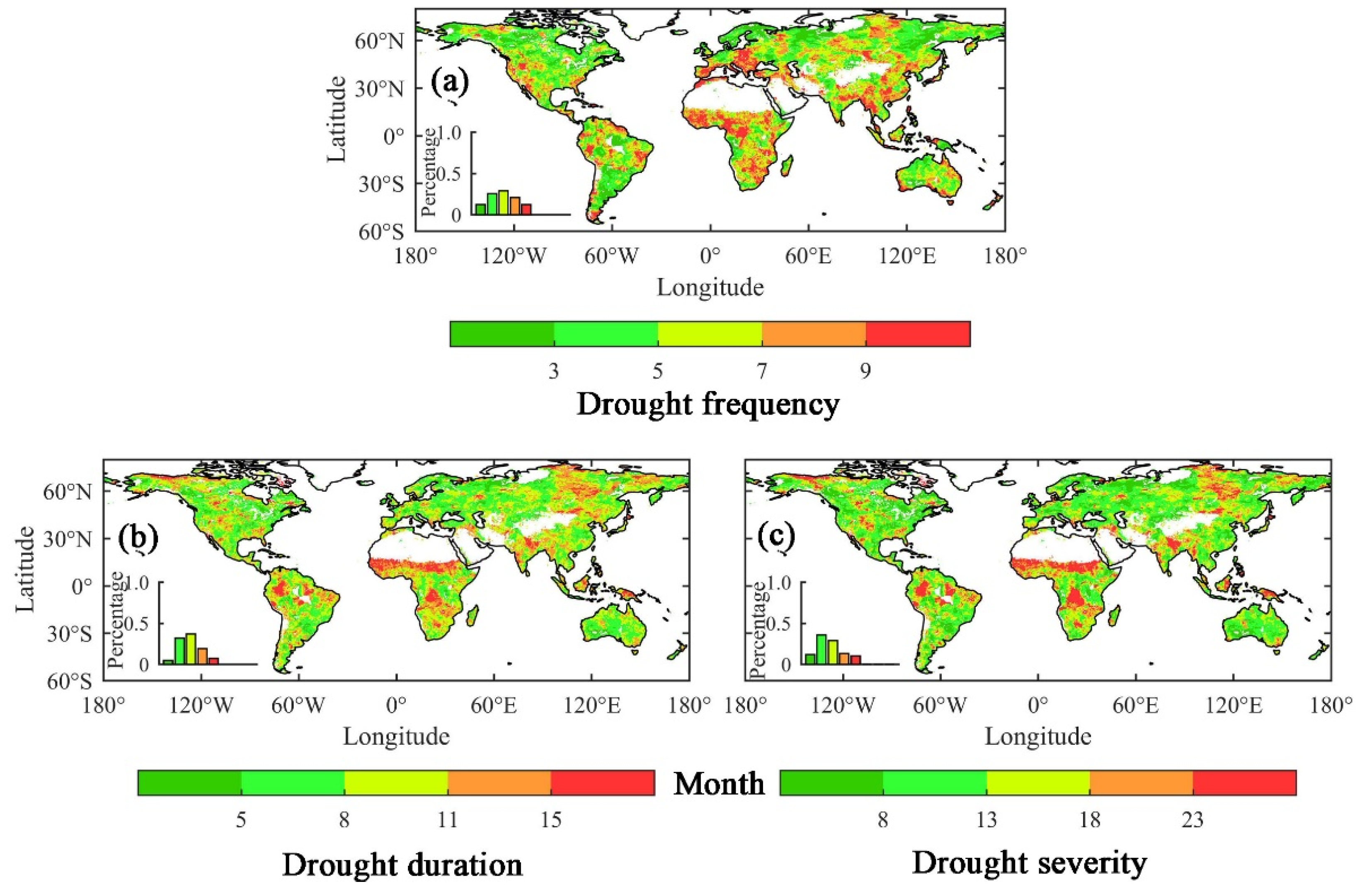
2.4. Identification of the Drought Events and Drought Characteristics

A drought event was defined as a period during which the drought index was below a predetermined truncation level. Based on the classification criteria of different drought levels corresponding to the different drought indices mentioned above, only negative values of these indicators may lead to drought events. In this study, a drought event was identified when the drought indices (including SPI-12, SPEI-12 and scPDSI) were less than or equal to −1 for at least three consecutive months and ended when drought indices were greater than −1. We defined the drought frequency as the number of drought events that occurred between 1982 and 2015 in each grid cell of the globe. For the drought events extracted in this study, the drought duration (D) was defined as a period (at least three continuous months) in which the drought index was below −1. Cumulated drought index during the drought duration was used to measure the magnitude of a drought event and called the drought severity (S) in this study (here, we take the opposite of S).

The duration and severity of all drought events in each grid on the globe were extracted from 1982 to 2015 based on above-mentioned three drought indices. We also extracted drought characteristics between 1982 and 2100 based on SPEI-12 (calculated by the mean of six models from the CMIP5 experiments). The Mann–Kendall test [50] was used to detect the trends of drought duration and drought severity between 1982 and 2100. Before constructing a joint drought duration and severity distribution by using copulas, we need to establish the optimal marginal distribution functions for drought duration and drought severity. In this study, we chose the extreme value (EV), generalized extreme value (GEV), exponential (EXP), gamma (GAM), Poisson (POISS), normal (NOR), generalized Pareto (GP) and Weibull (WBL) distribution functions as the candidate margins for drought duration and severity (Table S2). The F_D(d) and F_S(s) are assumed as the probability distribution functions of D and S, respectively, and the optimal F_D(d) and F_S(s) are established by the Kolmogorov–Smirnov (K-S) test [51]. The joint distribution function of F_D(d) and F_S(s) can be defined as a copula C:

$$F_{D,S}\left(d,s\right)=C\left(F_D\left(d\right),F_S\left(s\right)\right)$$

In this study, we used the methods of maximum likelihood and inference functions for margins to estimate the fit parameters in F_D(d), F_S(s) and F_D,S(d,s) [2]. The bivariate distribution functions commonly used, including Frank copula, Clayton copula, Gumbel copula, t copula and Normal copula, were constructed to coupled F_D(d) and F_S(s) in each pixel of the globe (as shown in Table S3). Then, we obtained the optimal joint distribution function of F_D(d) and F_S(s) by referring the method of the goodness of fit test given by Zhang et al. [2] and Berg [52].

2.5. Detecting the Response of Ecohydrological Variables to Drought

We evaluated the effect of drought on ecohydrological variables by calculating the anomalies in ecohydrological variables in drought period relative to non-drought period between 1982 and 2015. Partial correlation analysis was used to investigate the influence of different climate factors (including TMEP, RAD and SM) on NDVI and ET. In addition, we need to pay more attention to the degree of drought that can cause changes in ecohydrological variables. To examine whether the ecohydrological variables underwent significant changes during drought periods relative to non-drought periods, we adopted the Mann–Whitney–Wilcoxon test [53]. The drought thresholds were characterized by drought duration and drought severity when the drought caused the ecohydrological variables significant change. We used an example to clarify how threshold for ET response to drought at a given grid cell was identified. If there were 10 drought events at a given grid cell between 1982 and 2015, we first compared the change in ET values within each of these 10 drought events relative to the non-drought period. As not all drought events can cause significant changes in ET, the Mann–Whitney–Wilcoxon test was used to extract the drought events that caused significant changes in ET (p < 0.05) among the 10 drought events, and the corresponding drought event characteristics (including drought duration and drought severity) were counted. Then, the mean drought duration and drought severity of the drought events that caused significant changes were determined as the response threshold of ET to drought at that grid point (i.e., the duration and severity thresholds of drought that are sufficient to cause changes in ET). The same method was used to determine drought thresholds for other ecohydrological variables.

2.6. Evaluating the Occurrence Probability of Drought Events

Some important information for drought management can be obtained from the joint distribution function of multiple drought features. For example, the joint cumulative probability that both the drought duration and severity simultaneously up to certain values is recognized as a critical condition for a specific water-supply system and used to trigger a drought contingency plan [18]. In this study, we focused on the joint cumulative probability of drought duration and drought severity of drought events that can cause significant changes in ecohydrological variables. When the probability that both the drought duration and severity simultaneously exceed the thresholds for the response of ecohydrological variables to drought, drought will pose large threats to human and natural systems. We used the optimal joint distribution function of F_D(d) and F_S(s) constructed in each grid of the globe in Section 2.4 to estimate the occurrence probability of drought events that cause significant changes in ecohydrological variables in historical period (1982–2015) and project its change trend under future climate change (2011–2100). The change in occurrence probability (including joint cumulative probability and return period, calculated as follows) of drought events that cause changes in ecohydrological variables in the future (2011–2100) relative to historical period (1982–2015) will be used to evaluate the drought risk of ecohydrological variables under future climate change.

$$F\left(d,s\right)=P\left(D\le d,S\le s\right)={{\displaystyle \int }}_{-\infty }^s{{\displaystyle \int }}_{-\infty }^{d}f\left(s,d\right)d_u{d}_v$$

where d and s represent the drought duration and drought severity of drought events that cause significant changes in ecohydrological variables, respectively.

The return period of drought events that can cause ecohydrological variables significant changes in each grid of the globe were calculated, containing the joint return periods (T_α(d, s)) and cooccurrence return periods (T_β(d, s)) of D and S as follows:

$$\begin{array}{c}{T}_a\left(d,s\right)=\frac{N}{nP\left(D\ge d{\displaystyle \cup }S\ge s\right)}=\frac{N}{n\left(1-C\left(F_D\left(d\right),F_S\left(s\right)\right)\right)}\\ T_{\beta }\left(d,s\right)=\frac{N}{nP\left(D\ge d{\displaystyle \cap }S\ge s\right)}=\frac{N}{n\left(1-F_D\left(d\right)-F_S\left(s\right)+C\left(F_D\left(d\right),F_S\left(s\right)\right)\right)}\end{array}$$

where N is the length of the study period and n is the frequency of drought events.

3. Results

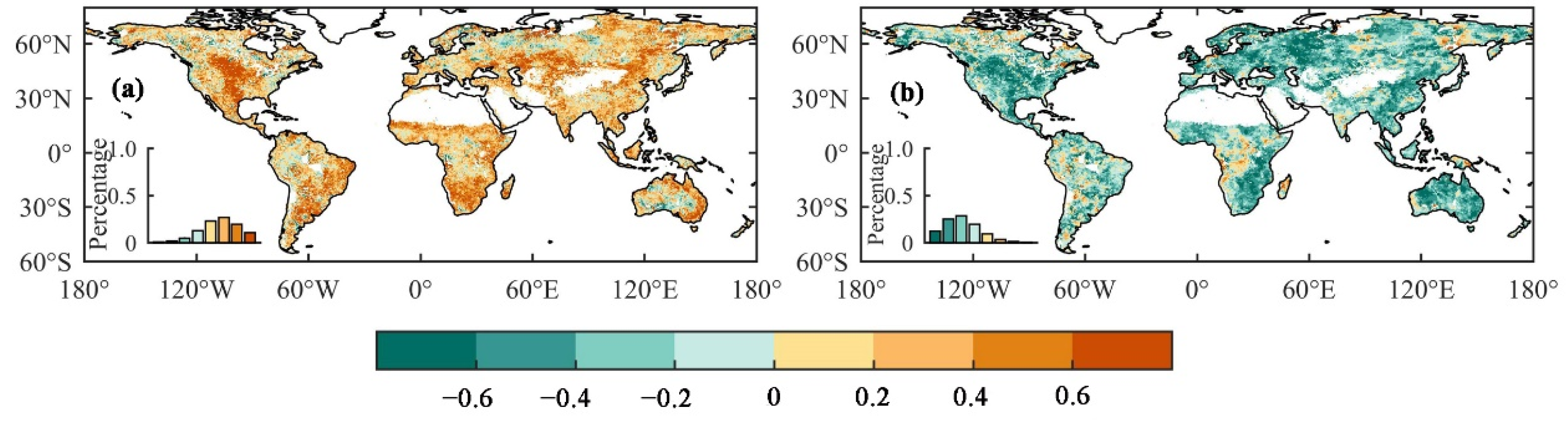
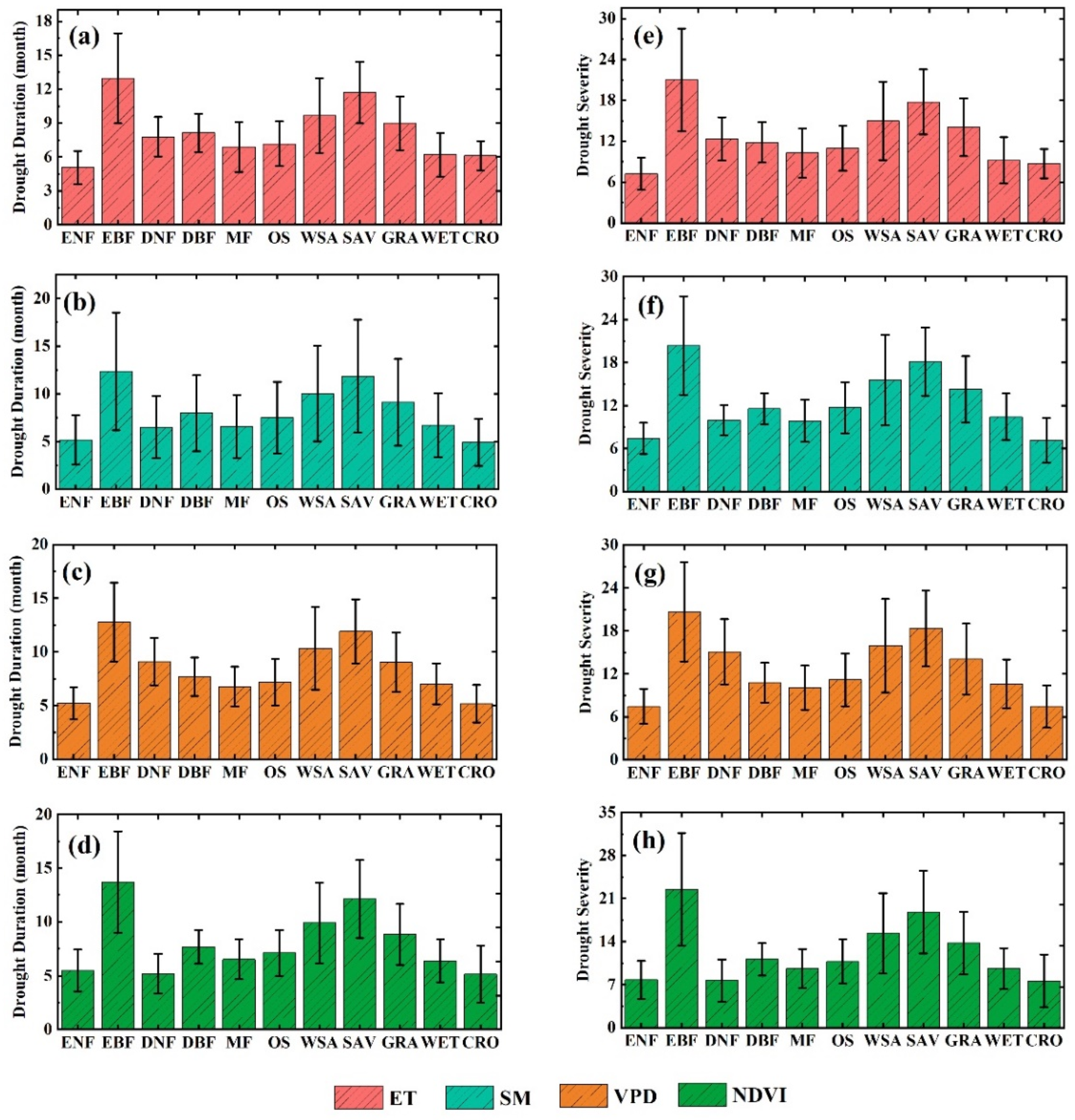
3.1. The Influence of Drought on Ecohydrological Variables

We counted the frequency of drought events, the average drought duration and the average drought severity that occurred between 1982 and 2015 in each grid of the globe base on SPI-12, SPEI-12 and scPDSI (as shown in Figure 1, Figures S2 and S3). Between 1982 and 2015, the drought hotspots according to drought frequency were located in the western United States, Venezuela, Colombia, eastern Brazil and southern Argentina in South America, southern Europe, central and southern Africa, central Russia, southeastern China and Myanmar and Laos. The average drought frequency of droughts in these regions can be more than nine times. The average drought duration and drought duration maps show similar spatial patterns as they are connected. The spatial patterns of drought frequency, average drought duration and severity counted based on SPEI-12 are consistent with SPI-12, while the main differences between scPDSI and SPI-12 (or SPEI-12) are in the western United States and mid-western Australia.

To evaluate the effect of drought on ecohydrological variables, we computed the anomalies in the ecohydrological variables in the drought period relative to the non-drought period between 1982 and 2015. The results show that, in the high latitudes of the Northern Hemisphere, eastern Asia, the Amazon Basin and central Africa, ET and NDVI increased under drought conditions (the areas with increased ET and NDVI accounted for 24.03% and 32.98% of the total global terrestrial vegetation land, respectively), while, in the other regions of the world, the occurrence of drought caused decreases in ET and NDVI (the area percentage were 75.97% and 67.02%, respectively) (Figure 2a,d). SM decreased in most regions of the global terrestrial vegetation land (93.47%) during the drought period, while VPD increased in 85.41% of the globe (Figure 2b,c). We further calculated the Spearman correlation coefficient of NDVI and ET, SM and VPD during the drought period based on SPI-12 between 1982 and 2015. The results show that NDVI was positively correlated with ET in 80.47% of the total global vegetation land (Figure 3a), and 85.23% of the regional SM was negatively correlated with VPD (Figure 3b). Consequently, it is apparent that a decrease in surface SM caused by drought is often accompanied by an increase in VPD in most parts of the world; a decrease (or increase) in NDVI in more than 80% of the total global vegetation land is often accompanied by a decrease (or increase) in ET during a drought period. The variation in ecohydrological variables during the drought period based on the SPEI-12 and scPDSI is consistent with that of the SPI-12 (Figures S4 and S5), indicating that the impact of drought on ecohydrological variables does not vary depending on the selected drought indicators.

Generally, due to the low water availability during drought periods, fewer water sources lead to a decrease in ET. At the same time, drought stress triggers plant stomata to partially close to minimize water loss, thereby reducing the vegetation transpiration. In addition, drought decreases NDVI through limiting photosynthesis (i.e., productivity). However, approximately 30% of the global ET and NDVI values increased after being disturbed by drought. To further reveal the cause of this phenomenon, we used partial correlation analysis to study the effects of temperature (TEMP), solar radiation (RAD) and precipitation (PRE) on ET and NDVI during the drought period. As shown in Figure 4a,b, TEMP and RAD play important roles in the changes in ET and NDVI in the high latitudes of the Northern Hemisphere, eastern Asia, the Amazon Basin and central Africa during the drought period, while, in other regions, ET and NDVI are mainly limited by PRE. In arid and semiarid areas, ET (or NDVI) is negatively correlated with TEMP and RAD (the mean correlation coefficients of ET with TEMP and RAD were −0.27 and −0.19, respectively, and the mean correlation coefficients of NDVI with TEMP and RAD were −0.04 and −0.05, respectively), while, in humid and semihumid areas, the opposite is true (the mean correlation coefficients of ET with TEMP and RAD were 0.05 and 0.14, respectively, and the mean correlation coefficients of NDVI with TEMP and RAD were 0.04 and 0.08, respectively). ET and NDVI are positively correlated with PRE globally (based on spatially averaged ET and NDVI, Figure 4c). At the same time, we also calculated the anomalies in climate factors (including TEMP, RAD and PRE) in the drought period relative to the non-drought period. As shown in Figure S6, we can observe that TEMP and RAD decreased in areas where ET and NDVI increased during the drought period, especially in the high latitudes of the Northern Hemisphere. Therefore, the increase in ET and NDVI in the high latitudes of the Northern Hemisphere is mainly caused by the decreased TEMP, and the TEMP and RAD in humid and semihumid regions play a dominant role in the change in ET and NDVI during the drought period. It has been shown that, in humid and semihumid areas, changes in TMEP and PRE during a drought period lead to a decrease in cloud cover, which promotes vegetation growth and a corresponding increase in evapotranspiration by absorbing more CO₂ [54]. In the area around the Bering Strait, the increase in ET/NDVI during the drought period is strongly correlated with the decrease in radiation, which may be related to the influence of the ocean circulation on the climate [55]. In contrast, in most parts of the world, ET and NDVI decreased during drought periods because of the increase in RAD and TEMP and the decrease in PRE.

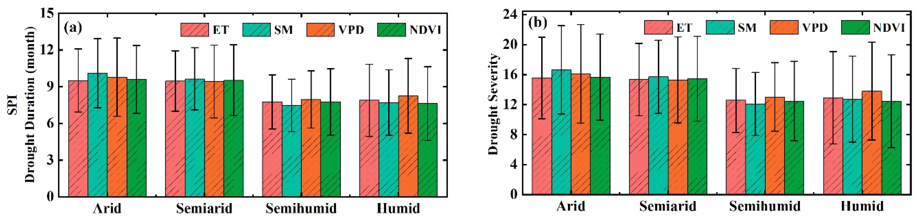
3.2. The Thresholds of Ecohydrological Variables in Response to Drought

We defined the thresholds of ecohydrological variables in response to drought as the extent to which drought can cause significant change in ecohydrological variables, characterized by drought duration and drought severity. The thresholds calculation of ecohydrological variables in response to drought refers to the examples given in the methodology. Therefore, we only extracted the drought events and corresponding drought features (drought duration and severity) that can lead to significant changes in ecohydrological variables at the grid cell level. As shown in Figure 5, the response thresholds for different ecohydrological variables to drought in the same area did not differ significantly (especially for ET, SM and VPD); i.e., when drought duration and drought severity can cause significant changes in one ecohydrological variable, other ecohydrological variables also change significantly under such drought characteristics. If a drought event lasted for 8 to 15 months and the corresponding drought severity reached the range of 10 to 20 (the opposite of the cumulative values of the drought index when the drought occurs), the drought would cause changes in the ecohydrological variables in more than half of the world. In western Europe, the northeastern part of North America and the southeastern part of Asia and South America, ecohydrological variables are more susceptible to drought disturbance. Generally, when a drought event lasts no more than 8 months, this drought process can cause changes in ET, SM, VPD and NDVI in the abovementioned areas. Based on SPEI-12 and scPDSI, the drought response thresholds of different ecohydrological variables in the same area are different from those based on SPI-12 (especially for scPDSI) but are consistent in their spatial distribution patterns (Figures S7 and S8).

Comparing the differences in the disturbance of ecohydrological variables caused by drought in various climatic regions, we found that different drought indicators showed that drought processes with longer duration and greater severity (the average drought duration and drought severity were 9.63 ± 2.78 months, 15.73 ± 5.60) could cause changes in ET, SM, VPD and NDVI in arid and semiarid regions compared to those in humid and semihumid regions (the average drought duration and drought severity were 7.80 ± 2.63 months, 12.77 ± 5.34). This significant discrepancy (p < 0.05) suggested that ecohydrological variables in humid and semihumid regions are more sensitive to drought (Figure 6 and Figure S9). To eliminate the impacts of high-intensity human activities on ecohydrological variables, we removed areas with high population densities (>10 persons/km²) based on the obtained population density data. The results consistently showed that humid and semihumid regions were more sensitive to drought (shorter duration and lower severity of drought event in semihumid and humid regions; the average drought duration and drought severity were 7.37± 2.62 months, 12.11 ± 5.39) than arid and semiarid regions (the average drought duration and drought severity were 9.20 ± 2.55 months, 14.89 ± 5.09) (Figure 7a,b, Figures S10a,b and S11a,b). At the same time, the durations and severities of drought events that caused disturbances to ecohydrological variables in areas with high population densities under the same climatic conditions were larger than those in areas with fewer human disturbances (Figure 7c,d, Figures S9c,d and S11c,d). We further assessed whether these differences were significant based on the Mann–Whitney–Wilcoxon test, and the results indicate that there were significant discrepancies in the response thresholds to drought for the same ecohydrological variable in the same condition under the influence of human activities (p < 0.05, Table S4), which means that high-intensity human activities in different climatic conditions increased the severity of drought processes. We further compared the differences in the response thresholds of ecohydrological variables to drought in rained croplands and irrigated croplands. The results show that the durations and severities of drought events that caused disturbances to ecohydrological variables in irrigated croplands regions (the average drought duration and drought severity were 11.08 ± 3.12 months, 18.10 ± 6.33) were larger than those in rained croplands regions (the average drought duration and drought severity were 10.84 ± 2.50 months, 17.38 ± 4.92) (as shown in Figure S12). We also assessed whether these differences were significant based on the Mann–Whitney–Wilcoxon test, and the results illustrated that there were significant discrepancies in the response thresholds to drought for the same ecohydrological variable between rained croplands and irrigated croplands (p < 0.05). Compared with rained croplands, irrigated croplands are more strongly affected by human activities, so the above results also indicated that high-intensity human activities can increase the severity of regional drought processes.

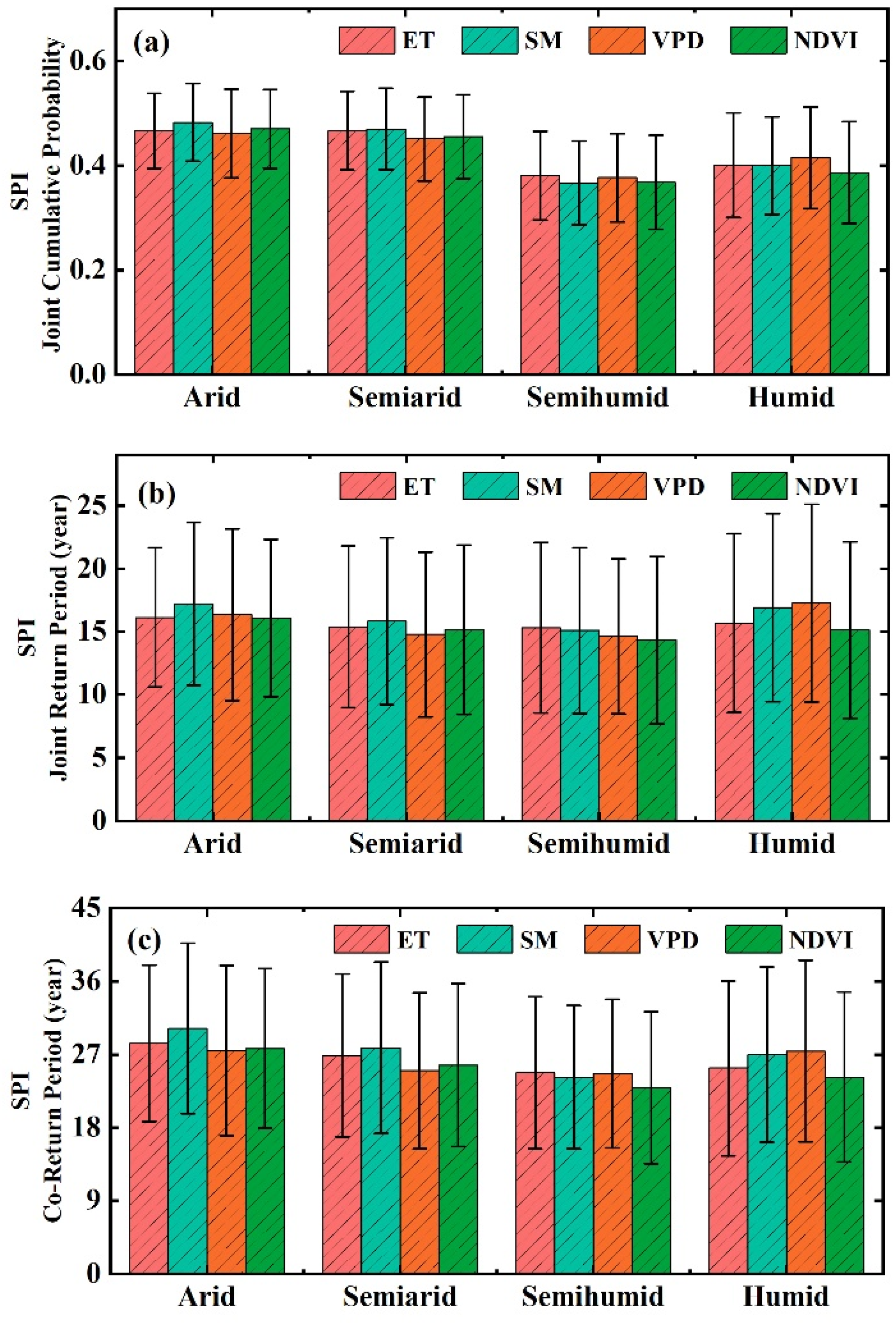
3.3. The Occurrence Probability of Drought Events That Can Cause Ecohydrological Variables Change

In this study, we focused on the occurrence probability of drought events that can cause significant changes in ecohydrological variables. When the probability is that both the drought duration and severity simultaneously exceed the thresholds for the response of ecohydrological variables to drought, drought will pose large threats to human and natural systems. Therefore, estimating the occurrence probability of drought events that cause significant changes in ecohydrological variables is important to facilitate the scientific prevention and mitigate the impact of drought on ecosystems. Before constructing a joint drought duration and severity distribution by using copulas, we need to establish the optimal marginal distribution functions for drought duration and drought severity. The optimal marginal distribution functions for drought duration and drought severity in each grid cell of the globe were fitted based on the K-S test (p ≤ 0.05, as shown in Figures S13 and S14a–f. Then, the optimal copula function with the drought duration and drought severity was fitted in each grid cell (Figure S14g–i), which was used to calculate the occurrence probability of drought events. The results illustrate that the joint cumulative probability of corresponding drought characteristics when different ecohydrological variables changes occurred was mainly concentrated in the range of 0.4 to 0.8 (based on SPI-12 and SPEI-12) (Figure S15a–h). For scPDSI, because the extracted drought process had a longer duration and higher drought severity, the joint cumulative probability increased, reaching more than 0.6 in more than 85% of the world (Figure S15i–l). In various climatic regions, the joint cumulative probability of the drought characteristics that caused changes in ecohydrological variables in humid and semihumid climate regions (the average joint cumulative probability was 0.38 ± 0.09) was lower than that in arid and semiarid regions; the average joint cumulative probability was 0.47 ± 0.07), mainly due to the humid and subhumid regions being more sensitive to drought (Figure 8a, Figures S18a and S19a).

Periodicity is a fundamental feature of natural disasters. Based on the joint cumulative probability and the frequency of droughts during the study period, we further studied the return periods of corresponding drought events when different ecohydrological variables changed. The shorter the return period, the more drought events occur that cause changes in ecohydrological variables in a given region. As shown in Figure S16, we found that, when the ecohydrological variables of eastern Asia, the Mediterranean coast, western North America, the Amazon River basin, eastern Australia and the northern and southern regions of Africa were disturbed by drought, similar drought processes occurred again in a short period of time (approximately 10 years), and these recurring drought events will have serious impacts on the local ecohydrological processes once again. The spatial distribution of the corresponding co-return period is consistent with that of the joint return period (Figure S17). Comparing the return periods of corresponding drought episodes after the ecohydrological variables in various climatic regions are disturbed by drought, it can be seen that there was no significant difference in the return period of drought events that cause changes in ecohydrological variables in various climatic zones; this is mainly attributed to the higher frequency of drought events in arid and semi-arid regions. The joint return period was within the range of 16.08 ± 1.77 years, and the corresponding co-recurrence period was 26.30 ± 2.63 years (Figure 8b,c, Figures S18b,c and S19b,c)

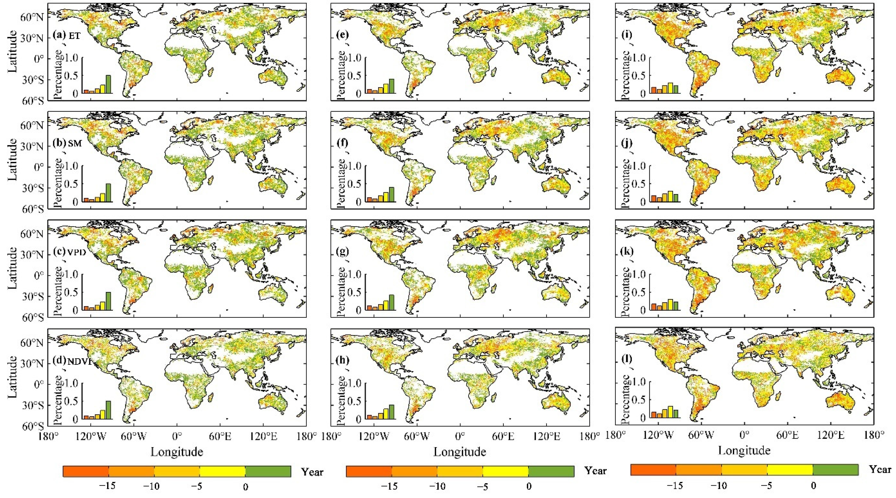
3.4. Drought Risk of Ecohydrological Variables in the Future

We analyzed the changes in joint cumulative probability and return period of drought characteristics that caused the changes in ecohydrological variables in the historical period (1982–2015) and in the future (2011–2040, 2041–2070 and 2071–2100). Note that, when the joint cumulative probability decreases and corresponding return period is shortened for a given region in the future, indicating that the drought risk of the ecohydrological variables in the area increases, and vice versa. As shown in Figure 9, the joint cumulative probabilities and return periods of the duration and severity of drought events that are expected to cause changes in ecohydrological variables in different climate regions under future climate scenarios show a significant downward trend. The joint cumulative probability of arid and semiarid regions decreased from 0.48 ± 0.07 in 1982–2015 to 0.33 ± 0.11 in 2071–2100, and the corresponding return period decreased from 15.29 ± 6.14 years to 8.70 ± 4.76 years. The joint cumulative probability of humid and semihumid areas decreased from 0.39 ± 0.09 in 1982–2015 to 0.32 ± 0.11 in 2071–2100, and the corresponding return period decreased from 13.71 ± 6.13 years to 8.90 ± 5.45 years. This phenomenon indicates that global ecohydrological variables will generally be more sensitive to drought in the future under the influence of climate change).

We further analyzed the relative changes in the joint return period at different stages in the future (2011–2040, 2041–2071 and 2071–2100) relative to the historical period (1982–2015). We found that, compared with the period from 1982 to 2015, the proportion of areas with shortened drought return periods in 2011–2040, 2041–2071 and 2071–2100 will gradually increase (Figure 10). Between 2071 and 2100, more than half of the world’s ecohydrological variables will be more susceptible to drought disturbances. The regions with shortened return periods of drought events that cause significant changes in ET, SM, VPD and NDVI account for 60.1%, 64.4%, 59.6% and 54.5% of the global land area, respectively, as shown in Figure 10i–l. Especially at the junction of Europe and Russia and in the central United States, the Amazon River Basin, southern Argentina, South Africa, southeastern China, Southeast Asia and most parts of Australia, higher frequencies of drought events that cause changes in ecohydrological variables under the background of global warming are expected. Ecosystem managers should conduct comprehensive management practices in response to global climate change based on the thresholds associated with significant changes in different ecohydrological variables caused by drought disturbances.

4. Discussion

4.1. Differences in the Influences of Various Drought Indicators on Ecohydrological Variables

Due to discrepancies in climate conditions in different regions, a single drought index may not provide more comprehensive and consistent drought information than results obtained by combining multiple drought indices [56,57]. Here, we chose the SPI considering precipitation only, the SPEI considering precipitation and evaporation demand and the scPDSI involving antecedent and current moisture supply and demand to capture all the drought episodes between 1982 and 2015. We found that the impact of drought on ecohydrological variables is not dependent on drought indicators. The changes in the ecohydrological variables in the drought period derived from three drought indices showed consistent spatial distribution characteristics (Figure 2, Figures S4 and S5); a decrease in surface SM caused by drought is often accompanied by an increase in VPD, while ET and NDVI are spatially consistent; that is, a decrease (or increase) in NDVI is often accompanied by a decrease (or increase) in ET during a drought period. This result stems from the similar variation trends of different drought indices used in this study. Wang et al. [58] also found SPI, SPEI and PDSI displayed high agreement spatial patterns of wetting/drying trends, especially in the Northern Hemisphere. The drought response thresholds of different ecohydrological variables in the same area derived from SPI are similar to SPEI, both in terms of variation amplitude and spatial distribution (Figure 5, Figure S7, Figure 7 and Figure S9a,b). However, ecohydrological variables had higher response thresholds to drought based on scPDSI, although it displayed similar spatial distribution patterns with SPI-12 and SPEI-12 (Figures S8 and S9c,d), which is mainly attributed to the extracted drought processes derived from scPDSI having longer durations and higher drought severities. In addition, the joint cumulative probabilities and return periods of drought events that caused changes in ecohydrological variables identified by different drought indicators also showed consistent variation amplitude and spatial distribution with drought thresholds (Figures S15–S17). Previous studies demonstrated that the SPI and SPEI have a superior capability compared to the PDSI to capture the drought impact on the ecohydrological variables because they can be calculated on various time scales [12,59]. Although we found that the SPI and the SPEI have similar results in characterizing drought’s impact on ecohydrological variables and their drought thresholds between 1982 and 2015, we recommend using the SPEI as a meteorological drought indicator to assess the impact of drought on ecosystems in the context of future global warming, which can further highlight the effect of temperature on drought [60,61].

4.2. Drought Thresholds of Ecohydrological Variables

Understanding ecosystem dynamics and predicting directional changes in ecosystems in response to extreme weather events is a continuous challenge in ecology. Previous studies have shown that there widely exists a threshold effect in ecosystem structure/functioning responses, such as photosynthesis, soil nitrogen and fungal abundance [62,63]. In this study, we identified the thresholds of ecohydrological variables (ET, SM, VPD and NDVI) in response to drought as the extent to which drought can cause a significant change in ecohydrological variables, characterized by drought duration and drought severity. The results illustrate that there was no significant difference in the spatial distribution of the response thresholds for different ecohydrological variables to drought (especially for ET, SM and VPD) (Figure 5, Figures S7 and S8). That is to say, when the drought causes significant changes in one ecohydrological variable, other ecohydrological variables are usually also strongly perturbed by this drought process. When the drought duration lasted for 8 to 15 months and the corresponding drought severity reached the range of 10 to 20, the drought would cause changes in ecohydrological variables in more than half of the world. Huang et al. [64] found that the persistence of a water deficit (11 months) with an intensity of −1.64 (SPEI) may lead to differential mortality of conifer species, which is consistent with our study results regarding the vegetation response to drought (Figure 5d,h and Figure S7d,h).

Various climate zones or biome types may have large differences in the extent and magnitude of water deficit required to cause negative impacts on ecohydrological variables [12,65]. Comparing the differences in the disturbances of ecohydrological variables caused by drought in various climatic regions, we found that different ecohydrological variables are more sensitive to drought in humid and semihumid regions regardless of which drought indicator is adopted (Figure 6 and Figure S9). On the one hand, arid and semiarid ecosystems can adapt well to water surplus/deficit [66]. Species in arid zones adapt to water scarcity through physiological, anatomical and functional strategies to reduce water loss, respiration costs, photosynthetic activity and growth rates [67,68]. Due to the arid and semiarid ecosystems having adapted to the long-term water deficit conditions, short-duration and low-severity droughts are unlikely to cause significant changes in ecohydrological variables [67]. On the other hand, the frequency of long-duration and high-severity drought events is higher in arid regions because of the limitation of water conditions [36]. Studies have shown that differences in biodiversity and soil texture in various climate regions can also affect the discrepancy in the response of ecohydrological variables to drought [69,70]. In addition, we also found that there were significant differences in the thresholds of ecohydrological variables’ response to drought in different biome types (Figure 11). It can be explained by the high correlation between biome distributions and climate zones. The thresholds of different vegetation types to drought from low to high was ENF, CRO, WET, MF, OS, DBF, DNF, GRA, WSA, SAV and EBF. There was also no obvious difference in the response degrees of the different ecohydrological variables to drought under the same vegetation type.

Studies have shown that anthropogenic activities (such as groundwater abstractions, reservoirs and mixed influences) were found to impact the duration, rate and timing of the recovery of drought events [71,72]. Our results illustrate that the durations and severities of drought events that caused disturbances to ecohydrological variables in areas with high population densities under the same climatic conditions were larger than those in areas with fewer human disturbances (Figure 7c,d, Figures S10c,d and S11c,d), indicating that high-intensity human activities increased the severity of drought processes. In addition, the durations and severities of drought events that caused disturbances to ecohydrological variables in irrigated croplands regions (the average drought duration and drought severity were 11.08 ± 3.12 months, 18.10 ± 6.33) were larger than those in rained croplands regions (the average drought duration and drought severity were 10.84 ± 2.50 months, 17.38 ± 4.92), and these discrepancies were significant (p < 0.05, based on Mann–Whitney–Wilcoxon test). Compared with rained croplands, irrigated croplands are more strongly affected by human activities, so the above results also indicate that high-intensity human activities can increase the severity of regional drought processes. These are in agreement with studies that human activities increased the average duration of drought termination and drought risk [71,72].

We also projected the occurrence probability’s change trend of drought events that cause changes in ecohydrological variables under future climate change. The results show that global ecohydrological variables will generally be more sensitive to drought in the future under the influence of climate change (Figure 9). The drought risk areas are mainly concentrated in the junction of Europe and Russia and in the central United States, the Amazon River Basin, southern Argentina, South Africa, southeastern China, southeast Asia and most parts of Australia in the future under the background of global warming (Figure 10). The duration and severity of future drought events will increase significantly in most parts of the world compared to historical periods, resulting in the frequent occurrence of high-intensity drought events and making more than half of the global vegetation area more prone to drought disturbances than the areas have been in the past (Figure 12).

4.3. The Limits of the Study

There are many uncertainties in different ecohydrological variables’ datasets (including satellite-derived, reanalysis and model simulations) due to varied forcing datasets and algorithms used [73]. For each ecohydrological variable, multiple datasets are currently available, and only one set of ecohydrological data was used in this study, which may cause some uncertainty in the results. We will further evaluate the variability of different data products in future work. The atmospheric and oceanic decadal variability (e.g., Pacific Decadal Oscillation) have an impact on ecohydrological variables [74], which may create some uncertainty in our results. In addition, in this study, we resampled all the datasets into 0.5° spatial resolution, which may also cause some uncertainty. We also made some efforts to reduce some uncertainties as much as possible. Due to ecohydrological variables not only being influenced by drought, we detrended and deseasonalized the time series of monthly ecohydrological variables to increase the robustness of the results.

5. Conclusions

This article revealed the extent and magnitude of meteorological drought in terms of causing changes in ecohydrological variables (including ET, SM, VPD and NDVI) and projected the occurrence probability’s change trend of drought events that cause changes in ecohydrological variables under future climate change. The results show that the impact of drought on ecohydrological variables is not dependent on drought indicators. SM decreased significantly in most regions of the world (93.47%) during the drought period, while VPD increased in 85.41% of the globe. ET and NDVI were expected to decrease in most parts of the world due to increases in RAD and TEMP and decreases in SM during drought periods. There was no obvious difference in the response degrees of the different ecohydrological variables to drought in the same area. If a drought event lasted for 8 to 15 months and the corresponding drought severity reached the range of 10 to 20, the drought would cause changes in the ecohydrological variables in more than half of the world. Ecohydrological variables are more sensitive to drought in humid and semihumid regions regardless of which drought indicator is adopted. The joint return period of drought events that cause changes in ecohydrological variables was within the range of 16.08 ± 1.77 years. Between 2071 and 2100, more than half of the world’s ecohydrological variables are expected to be more susceptible to drought disturbances (regions with shorter return periods of drought events that cause significant changes in ET, SM, VPD and NDVI account for 60.1%, 64.4%, 59.6% and 54.5% of the global land area, respectively). Although certain uncertainties still exist, our findings provide some theoretical and practical reference for policy development and ecosystem management.

References

1. Etkin, D.; Medalye, J.; Higuchi, K. Climate warming and natural disaster management: An exploration of the issues. Clim. Chang. 2012, 112, 585–599. [Google Scholar] [CrossRef]
2. Zhang, Y.; Feng, X.; Wang, X.; Fu, B. Characterizing drought in terms of changes in the precipitation–runoff relationship: A case study of the Loess Plateau, China. Hydrol. Earth Syst. Sci. 2018, 22, 1749–1766. [Google Scholar] [CrossRef] [Green Version]
3. Alfieri, L.; Burek, P.; Feyen, L.; Forzieri, G. Global warming increases the frequency of river floods in Europe. Hydrol. Earth Syst. Sci. 2015, 19, 2247–2260. [Google Scholar] [CrossRef] [Green Version]
4. Chen, Y.; Li, Z.; Li, W.; Deng, H.; Shen, Y. Water and ecological security: Dealing with hydroclimatic challenges at the heart of China’s Silk Road. Environ. Earth Sci. 2016, 75, 881. [Google Scholar] [CrossRef]
5. Cook, B.I.; Smerdon, J.E.; Seager, R.; Coats, S. Global warming and 21st century drying. Clim. Dyn. 2014, 43, 2607–2627. [Google Scholar] [CrossRef] [Green Version]
6. Vose, J.M.; Miniat, C.F.; Luce, C.H.; Asbjornsen, H.; Caldwell, P.V.; Campbell, J.L.; Grant, G.E.; Isaak, D.J.; Loheide, S.P., II; Sun, G. Ecohydrological implications of drought for forests in the United States. For. Ecol. Manag. 2016, 380, 335–345. [Google Scholar] [CrossRef] [Green Version]
7. Seneviratne, S.I.; Corti, T.; Davin, E.L.; Hirschi, M.; Jaeger, E.B.; Lehner, I.; Orlowsky, B.; Teuling, A.J. Investigating soil moisture—Climate interactions in a changing climate: A review. Earth-Sci. Rev. 2010, 99, 125–161. [Google Scholar] [CrossRef]
8. Hashimoto, H.; Dungan, J.; White, M.; Yang, F.; Michaelis, A.; Running, S.; Nemani, R. Satellite-based estimation of surface vapor pressure deficits using MODIS land surface temperature data. Remote Sens. Environ. 2008, 112, 142–155. [Google Scholar] [CrossRef]
9. He, M.; Kimball, J.S.; Running, S.; Ballantyne, A.; Guan, K.; Huemmrich, F. Satellite detection of soil moisture related water stress impacts on ecosystem productivity using the MODIS-based photochemical reflectance index. Remote Sens. Environ. 2016, 186, 173–183. [Google Scholar] [CrossRef] [Green Version]
10. Cai, J.; Liu, Y.; Lei, T.; Pereira, L.S. Estimating reference evapotranspiration with the FAO Penman–Monteith equation using daily weather forecast messages. Agric. For. Meteorol. 2007, 145, 22–35. [Google Scholar] [CrossRef]
11. Joiner, J.; Yoshida, Y.; Anderson, M.; Holmes, T.; Hain, C.; Reichle, R.; Koster, R.; Middleton, E.; Zeng, F.-W. Global relationships among traditional reflectance vegetation indices (NDVI and NDII), evapotranspiration (ET), and soil moisture variability on weekly timescales. Remote Sens. Environ. 2018, 219, 339–352. [Google Scholar] [CrossRef] [PubMed] [Green Version]
12. Vicente-Serrano, S.M.; Gouveia, C.; Camarero, J.J.; Beguería, S.; Trigo, R.; López-Moreno, J.I.; Azorín-Molina, C.; Pasho, E.; Lorenzo-Lacruz, J.; Revuelto, J.; et al. Response of vegetation to drought time-scales across global land biomes. Proc. Natl. Acad. Sci. USA 2013, 110, 52–57. [Google Scholar] [CrossRef] [PubMed] [Green Version]
13. van Schaik, E.; Killaars, L.; Smith, N.E.; Koren, G.; Van Beek, L.; Peters, W.; van der Laan-Luijkx, I.T. Changes in surface hydrology, soil moisture and gross primary production in the Amazon during the 2015/2016 El Niño. Philos. Trans. R. Soc. B Biol. Sci. 2018, 373, 20180084. [Google Scholar] [CrossRef] [PubMed]
14. Anderegg, W.R.L.; Kane, J.M.; Anderegg, L.D.L. Consequences of widespread tree mortality triggered by drought and temperature stress. Nat. Clim. Chang. 2012, 3, 30–36. [Google Scholar] [CrossRef]
15. Liu, L.; Gudmundsson, L.; Hauser, M.; Qin, D.; Li, S.; Seneviratne, S.I. Soil moisture dominates dryness stress on ecosystem production globally. Nat. Commun. 2020, 11, 4892. [Google Scholar] [CrossRef]
16. Ma, Z.; Lei, X.; Zhu, Q.; Chen, H.; Peng, C. A drought-induced pervasive increase in tree mortality across Canada’s boreal forests. Nat. Clim. Chang. 2011, 1, 467–471. [Google Scholar]
17. Mukherjee, S.; Mishra, A.; Trenberth, K.E. Climate Change and Drought: A Perspective on Drought Indices. Curr. Clim. Chang. Rep. 2018, 4, 145–163. [Google Scholar] [CrossRef]
18. Shiau, J. Fitting Drought Duration and Severity with Two-Dimensional Copulas. Water Resour. Manag. 2006, 20, 795–815. [Google Scholar] [CrossRef]
19. Yusof, F.; Hui-Mean, F.; Suhaila, J.; Yusof, Z. Characterisation of Drought Properties with Bivariate Copula Analysis. Water Resour. Manag. 2013, 27, 4183–4207. [Google Scholar] [CrossRef]
20. Xu, K.; Yang, D.; Xu, X.; Lei, H. Copula based drought frequency analysis considering the spatio-temporal variability in Southwest China. J. Hydrol. 2015, 527, 630–640. [Google Scholar] [CrossRef]
21. Nabaei, S.; Sharafati, A.; Yaseen, Z.M.; Shahid, S. Copula based assessment of meteorological drought characteristics: Regional investigation of Iran. Agric. For. Meteorol. 2019, 276–277, 107611. [Google Scholar] [CrossRef]
22. Bárdossy, A. Copula-based geostatistical models for groundwater quality parameters. Water Resour. Res. 2006, 42, W11416. [Google Scholar] [CrossRef]
23. Borgomeo, E.; Pflug, G.; Hall, J.W.; Hochrainer-Stigler, S. Assessing water resource system vulnerability to unprecedented hydrological drought using copulas to characterize drought duration and deficit. Water Resour. Res. 2015, 51, 8927–8948. [Google Scholar] [CrossRef] [PubMed] [Green Version]
24. Salvadori, G.; De Michele, C. Multivariate multiparameter extreme value models and return periods: A copula approach. Water Resour. Res. 2010, 46, W10501. [Google Scholar] [CrossRef]
25. AghaKouchak, A.; Cheng, L.; Mazdiyasni, O.; Farahmand, A. Global warming and changes in risk of concurrent climate extremes: Insights from the 2014 California drought. Geophys. Res. Lett. 2014, 41, 8847–8852. [Google Scholar] [CrossRef] [Green Version]
26. Madadgar, S.; AghaKouchak, A.; Farahmand, A.; Davis, S.J. Probabilistic estimates of drought impacts on agricultural production. Geophys. Res. Lett. 2017, 44, 7799–7807. [Google Scholar] [CrossRef]
27. Guo, Y.; Huang, S.; Huang, Q.; Wang, H.; Wang, L.; Fang, W. Copulas-based bivariate socioeconomic drought dynamic risk assessment in a changing environment. J. Hydrol. 2019, 575, 1052–1064. [Google Scholar] [CrossRef]
28. Fang, W.; Huang, S.; Huang, Q.; Huang, G.; Wang, H.; Leng, G.; Wang, L.; Guo, Y. Probabilistic assessment of remote sensing-based terrestrial vegetation vulnerability to drought stress of the Loess Plateau in China. Remote Sens. Environ. 2019, 232, 111290. [Google Scholar] [CrossRef]
29. Wilhite, D.A.; Glantz, M.H. Understanding: The Drought Phenomenon: The Role of Definitions. Water Int. 1985, 10, 111–120. [Google Scholar] [CrossRef] [Green Version]
30. Hao, Z.; AghaKouchak, A.; Nakhjiri, N.; Farahmand, A. Global integrated drought monitoring and prediction system. Sci. Data 2014, 1, 140001. [Google Scholar] [CrossRef]
31. Kogan, F.N. Remote sensing of weather impacts on vegetation in non-homogeneous areas. Int. J. Remote Sens. 1990, 11, 1405–1419. [Google Scholar] [CrossRef]
32. McKee, T.B.; Doesken, N.J.; Kleist, J. The relationship of drought frequency and duration to time scales. In Proceedings of the 8th Conference on Applied Climatology, Boston, MA, USA, 17–22 January 1993; pp. 179–183. [Google Scholar]
33. Vicente-Serrano, S.M.; Beguería, S.; López-Moreno, J.I. A Multiscalar Drought Index Sensitive to Global Warming: The Standardized Precipitation Evapotranspiration Index. J. Clim. 2010, 23, 1696–1718. [Google Scholar] [CrossRef] [Green Version]
34. Beguería, S.; Vicente-Serrano, S.M.; Reig, F.; Latorre, B. Standardized precipitation evapotranspiration index (SPEI) revisited: Parameter fitting, evapotranspiration models, tools, datasets and drought monitoring. Int. J. Clim. 2014, 34, 3001–3023. [Google Scholar] [CrossRef] [Green Version]
35. Trenberth, K.E.; Dai, A.; Van Der Schrier, G.; Jones, P.D.; Barichivich, J.; Briffa, K.R.; Sheffield, J. Global warming and changes in drought. Nat. Clim. Chang. 2013, 4, 17–22. [Google Scholar] [CrossRef]
36. Spinoni, J.; Naumann, G.; Carrao, H.; Barbosa, P.; Vogt, J. World drought frequency, duration, and severity for 1951–2010. Int. J. Clim. 2014, 34, 2792–2804. [Google Scholar] [CrossRef] [Green Version]
37. Harris, I.; Jones, P.D.; Osborn, T.J.; Lister, D.H. Updated high-resolution grids of monthly climatic observations–the CRU TS3. 10 Dataset. Int. J. Climatol. 2014, 34, 623–642. [Google Scholar] [CrossRef] [Green Version]
38. Detwiler, A. Extrapolation of the Goff-Gratch Formula for Vapor Pressure of Liquid Water at Temperatures Below 0 °C. J. Clim. Appl. Meteorol. 1983, 22, 503–504. [Google Scholar] [CrossRef] [Green Version]
39. Viovy, N. CRUNECP Version 7-Atmospheric Forcing Data for the Community Land Model; Research Data Archive at the National Center for Atmospheric Research, Computational and Information Systems Laboratory: Boulder, CO, USA, 2018; Available online: https://rda.ucar.edu/datasets/ds314.3/ (accessed on 10 January 2021).
40. Gribbon, K.T.; Bailey, D.G. A novel approach to real-time bilinear interpolation. In Proceedings of the IEEE International Workshop on Electronic Design, Perth, WA, Australia, 26–31 January 2004. [Google Scholar]
41. Pinzon, J.E.; Tucker, C.J. A non-stationary 1981–2012 AVHRR NDVI3g time series. Remote Sens. 2014, 6, 6929–6960. [Google Scholar] [CrossRef] [Green Version]
42. Holben, B.N. Characteristics of maximum-value composite images from temporal AVHRR data. Int. J. Remote Sens. 2007, 7, 1417–1434. [Google Scholar] [CrossRef]
43. Friedl, M.A.; Sulla-Menashe, D.; Tan, B.; Schneider, A.; Ramankutty, N.; Sibley, A.; Huang, X. MODIS Collection 5 global land cover: Algorithm refinements and characterization of new datasets. Remote Sens. Environ. 2010, 114, 168–182. [Google Scholar] [CrossRef]
44. Martens, B.; Gonzalez Miralles, D.; Lievens, H.; Van Der Schalie, R.; De Jeu, R.A.M.; Fernández-Prieto, D.; Beck, H.E.; Dorigo, W.A.; Verhoest, N.E.C. GLEAM v3: Satellite-based land evaporation and root-zone soil moisture. Geosci. Model Dev. 2017, 10, 1903–1925. [Google Scholar] [CrossRef] [Green Version]
45. Doxsey-Whitfield, E.; MacManus, K.; Adamo, S.B.; Pistolesi, L.; Squires, J.; Borkovska, O.; Baptista, S.R. Taking Advantage of the Improved Availability of Census Data: A First Look at the Gridded Population of the World, Version 4. Pap. Appl. Geogr. 2015, 1, 226–234. [Google Scholar] [CrossRef]
46. Chen, Y.; Feng, X.; Fu, B.; Shi, W.; Yin, L.; Lv, Y. Recent Global Cropland Water Consumption Constrained by Observations. Water Resour. Res. 2019, 55, 3708–3738. [Google Scholar] [CrossRef]
47. van der Schrier, G.; Jones, P.D.; Briffa, K.R. The sensitivity of the PDSI to the Thornthwaite and Penman-Monteith parameterizations for potential evapotranspiration. J. Geophys. Res. Earth Surf. 2011, 116, D03106. [Google Scholar] [CrossRef]
48. Feng, S.; Fu, Q. Expansion of global drylands under a warming climate. Atmos. Chem. Phys. 2013, 13, 10081–10094. [Google Scholar] [CrossRef] [Green Version]
49. Kafle, H.; Bruins, H.J. Climatic trends in Israel 1970–2002: Warmer and increasing aridity inland. Clim. Chang. 2009, 96, 63–77. [Google Scholar] [CrossRef]
50. Mann, H.B. Nonparametric test against trend. Econometrica 1945, 13, 245–259. [Google Scholar] [CrossRef]
51. Massey, F.J. The Kolmogorov-Smirnov Test for Goodness of Fit. J. Am. Stat. Assoc. 1951, 46, 68–78. [Google Scholar] [CrossRef]
52. Berg, D. Copula goodness-of-fit testing: An overview and power comparison. Eur. J. Financ. 2009, 15, 675–701. [Google Scholar] [CrossRef]
53. Swain, S.; Hayhoe, K. CMIP5 projected changes in spring and summer drought and wet conditions over North America. Clim. Dyn. 2015, 44, 2737–2750. [Google Scholar] [CrossRef]
54. Bonal, D.; Bosc, A.; Ponton, S.; Goret, J.Y.; Burban, B.; Gross, P.; Bonnefond, J.M.; Elbers, J.; Longdoz, B.; Epron, D.; et al. Impact of severe dry season on net ecosystem exchange in the Neotropical rainforest of French Guiana. Glob. Chang. Biol. 2008, 14, 1917–1933. [Google Scholar] [CrossRef]
55. Winton, M.; Griffies, S.M.; Samuels, B.L.; Sarmiento, J.L.; Frölicher, T.L. Connecting Changing Ocean Circulation with Changing Climate. J. Clim. 2013, 26, 2268–2278. [Google Scholar] [CrossRef]
56. Adnan, S.; Ullah, K.; Shuanglin, L.; Gao, S.; Khan, A.H.; Mahmood, R. Comparison of various drought indices to monitor drought status in Pakistan. Clim. Dyn. 2018, 51, 1885–1899. [Google Scholar] [CrossRef]
57. Chen, S.; Gan, T.Y.; Tan, X.; Shao, D.; Zhu, J. Assessment of CFSR, ERA-Interim, JRA-55, MERRA-2, NCEP-2 reanalysis data for drought analysis over China. Clim. Dyn. 2019, 53, 737–757. [Google Scholar] [CrossRef]
58. Wang, H.; He, B.; Zhang, Y.; Huang, L.; Chen, Z.; Liu, J. Response of ecosystem productivity to dry/wet conditions indicated by different drought indices. Sci. Total Environ. 2018, 612, 347–357. [Google Scholar] [CrossRef] [PubMed]
59. Xu, H.-J.; Wang, X.-P.; Zhao, C.-Y.; Shan, S.-Y.; Guo, J. Seasonal and aridity influences on the relationships between drought indices and hydrological variables over China. Weather Clim. Extrem. 2021, 34, 100393. [Google Scholar] [CrossRef]
60. Tomas-Burguera, M.; Vicente-Serrano, S.M.; Peña-Angulo, D.; Domínguez-Castro, F.; Noguera, I.; El Kenawy, A. Global characterization of the varying responses of the standardized precipitation evapotranspiration index to atmospheric evaporative demand. J. Geophys. Res. Atmos. 2020, 125, e2020JD033017. [Google Scholar] [CrossRef]
61. Yang, S.; Zhang, J.; Han, J.; Wang, J.; Zhang, S.; Bai, Y.; Cao, D.; Xun, L.; Zheng, M.; Chen, H.; et al. Evaluating global ecosystem water use efficiency response to drought based on multi-model analysis. Sci. Total Environ. 2021, 778, 146356. [Google Scholar] [CrossRef]
62. Berdugo, M.; Delgado-Baquerizo, M.; Soliveres, S.; Hernández-Clemente, R.; Zhao, Y.; Gaitán, J.J.; Gross, N.; Saiz, H.; Maire, V.; Lehmann, A.; et al. Global ecosystem thresholds driven by aridity. Science 2020, 367, 787–790. [Google Scholar] [CrossRef] [Green Version]
63. Munson, S.M.; Reed, S.C.; Peñuelas, J.; McDowell, N.G.; Sala, O. Ecosystem thresholds, tipping points, and critical transitions. New Phytol. 2018, 218, 1315–1317. [Google Scholar] [CrossRef]
64. Huang, K.; Yi, C.; Wu, D.; Zhou, T.; Zhao, X.; Blanford, W.J.; Wei, S.; Wu, H.; Ling, D.; Li, Z. Tipping point of a conifer forest ecosystem under severe drought. Environ. Res. Lett. 2015, 10, 024011. [Google Scholar] [CrossRef]
65. Zhang, Y.; Feng, X.; Fu, B.; Chen, Y.; Wang, X. Satellite-Observed Global Terrestrial Vegetation Production in Response to Water Availability. Remote Sens. 2021, 13, 1289. [Google Scholar] [CrossRef]
66. Schwinning, S.; Sala, O.E. Hierarchy of responses to resource pulses in arid and semi-arid ecosystems. Oecologia 2004, 141, 211–220. [Google Scholar] [CrossRef] [PubMed]
67. Chaves, M.M.; Maroco, J.P.; Pereira, J.S. Understanding plant responses to drought—From genes to the whole plant. Funct. Plant Biol. 2003, 30, 239–264. [Google Scholar] [CrossRef]
68. Lundholm, B. Adaptations in arid ecosystems. Can Dessert Encroachment be Stopped? Ecological Bull. 1976, 19–27. [Google Scholar]
69. Rostampour, M.; Saghari, M. Evaluating Drought Effects on Soil Properties and Plant Species Diversity of Amiodendron Persicum Reserve in Haji Abad Rangelands, South Khorasan. Desert Ecosyst. Eng. J. 2020, 9, 87–102. [Google Scholar]
70. Jiang, P.; Ding, W.; Yuan, Y.; Ye, W. Diverse response of vegetation growth to multi-time-scale drought under different soil textures in China’s pastoral areas. J. Environ. Manag. 2020, 274, 110992. [Google Scholar] [CrossRef]
71. Diffenbaugh, N.S.; Swain, D.L.; Touma, D. Anthropogenic warming has increased drought risk in California. Proc. Natl. Acad. Sci. USA 2015, 112, 3931–3936. [Google Scholar] [CrossRef] [Green Version]
72. Margariti, J.; Rangecroft, S.; Parry, S.; Wendt, D.; Van Loon, A.; Chadwick, O. Anthropogenic activities alter drought termination. Elem. Sci. Anthr. 2019, 7, 27. [Google Scholar] [CrossRef] [Green Version]
73. Liu, W.; Sun, F.; Sun, S.; Guo, L.; Wang, H.; Cui, H. Multi-scale assessment of eco-hydrological resilience to drought in China over the last three decades. Sci. Total Environ. 2019, 672, 201–211. [Google Scholar] [CrossRef]
74. Salas, H.D.; Poveda, G.; Mesa, Ó.J.; Marwan, N. Generalized Synchronization between ENSO and Hydrological Variables in Colombia: A Recurrence Quantification Approach. Front. Appl. Math. Stat. 2020, 6, 3. [Google Scholar] [CrossRef]
Figure 1. Spatial distribution of drought frequency (a), average drought duration (b) and average drought severity (c) between 1982 and 2015 based on SPI-12. Water, barren land and regions without any relevant drought events were masked.
Remotesensing 14 01920 g001
Figure 2. Changes in ecohydrological variables during the drought period based on SPI-12. (ad) show the anomalies in ET, SM, VPD and NDVI, respectively, in the drought period compared to those in the non-drought period. Water, barren land and regions without any relevant drought events were masked.
Remotesensing 14 01920 g002
Figure 3. The spatial patterns of the Spearman correlation coefficient between NDVI and ET (a), SM and VPD (b) during the drought period based on SPI-12 from 1982 to 2015. Water, barren land and regions without any relevant drought events were masked.
Remotesensing 14 01920 g003
Figure 4. Spatial distribution of the influence of potential climate factors (TEMP, RAD and PRE) on (a) ET and (b) NDVI during the 1982–2015 drought period, (c) Spearman correlation coefficients of average ET (or NDVI) and potential climate factors (TEMP, RAD and PRE) in different climate regions. The error bars indicate ±1 standard error. Water, barren land and regions without any relevant drought events were masked.
Remotesensing 14 01920 g004
Figure 5. Spatial patterns of drought thresholds (characterized by drought duration and drought severity) when the drought caused the ecohydrological variables change (SPI-12). The left and right columns show the results for the drought duration (ad) and drought severity (eh), respectively. The rows from top to bottom represent ET, SM, VPD and NDVI, respectively. Water, barren land and regions without any relevant drought events were masked.
Remotesensing 14 01920 g005
Figure 6. Drought thresholds (characterized by drought duration (a) and drought severity (b)) when the drought caused the ecohydrological variables change in different climate regions. The error bars indicate ±1 standard error.
Remotesensing 14 01920 g006
Figure 7. Drought thresholds (characterized by drought duration and drought severity) in various climate regions (excluding regions with high population densities (population density > 10/km2, (a,b)). (c,d) represent the relative changes in drought thresholds in various climate regions (thresholds in whole study area minus thresholds in areas with low population densities)). The error bars indicate ±1 standard error.
Remotesensing 14 01920 g007
Figure 8. The joint cumulative probabilities (a) and return periods (b,c) of drought characteristics when the ecohydrological variables changes were caused by drought in various climate regions (SPI-12). The error bars indicate ±1 standard error.
Remotesensing 14 01920 g008
Figure 9. Changes in the joint cumulative probabilities (ad) and joint return periods (eh) of corresponding drought characteristics when the ecohydrological variables change in various climate regions. Each climate zone represents the joint cumulative probability and joint return period values of ET, SM, VPD and NDVI in the four time periods of 1982–2015, 2011–2040, 2041–2070 and 2071–2100. The error bars indicate ±1 standard error.
Remotesensing 14 01920 g009
Figure 10. The spatial distribution of changes in the joint return period at different stages in the future relative to the historical period. The left, middle and right columns show the changes in the joint return periods 2011–2040 (ad), 2041–2070 (eh) and 2071–2100 (il) relative to 1982–2015, respectively. The rows represent, from top to bottom, ET, SM, VPD and NDVI, respectively. Water, barren land and regions without any relevant drought events were masked.
Remotesensing 14 01920 g010
Figure 11. Drought thresholds (characterized by drought duration (ad) and drought severity (eh)) of ecohydrological variables in different biome types. The error bars indicate ±1 standard error.
Remotesensing 14 01920 g011
Figure 12. Spatial distribution of trends in drought duration (a) and drought severity (b) over the period 1982–2100 (black “+” indicates the trend is statistically significant at the 5% level).
Remotesensing 14 01920 g012
Publisher’s Note: MDPI stays neutral with regard to jurisdictional claims in published maps and institutional affiliations.