Abstract
Caatinga biome, located in the Brazilian semi-arid region, is the most populous semi-arid region in the world, causing intensification in land degradation and loss of biodiversity over time. The main objective of this paper is to determine and analyze the changes in land cover and use, over time, on the biophysical parameters in the Caatinga biome in the semi-arid region of Brazil using remote sensing. Landsat-8 images were used, along with the Surface Energy Balance Algorithm for Land (SEBAL) in the Google Earth Engine platform, from 2013 to 2019, through spatiotemporal modeling of vegetation indices, i.e., leaf area index (LAI) and vegetation cover (VC). Moreover, land surface temperature (LST) and actual evapotranspiration (ETa) in Petrolina, the semi-arid region of Brazil, was used. The principal component analysis was used to select descriptive variables and multiple regression analysis to predict ETa. The results indicated significant effects of land use and land cover changes on energy balances over time. In 2013, 70.2% of the study area was composed of Caatinga, while the lowest percentages were identified in 2015 (67.8%) and 2017 (68.7%). Rainfall records in 2013 ranged from 270 to 480 mm, with values higher than 410 mm in 46.5% of the study area, concentrated in the northern part of the municipality. On the other hand, in 2017 the lowest annual rainfall values (from 200 to 340 mm) occurred. Low vegetation cover rate was observed by LAI and VC values, with a range of 0 to 25% vegetation cover in 52.3% of the area, which exposes the effects of the dry season on vegetation. The highest LST was mainly found in urban areas and/or exposed soil. In 2013, 40.5% of the region’s area had LST between 48.0 and 52.0 °C, raising ETa rates (~4.7 mm day−1). Our model has shown good outcomes in terms of accuracy and concordance (coefficient of determination = 0.98, root mean square error = 0.498, and Lin’s concordance correlation coefficient = 0.907). The significant increase in agricultural areas has resulted in the progressive reduction of the Caatinga biome. Therefore, mitigation and sustainable planning is vital to decrease the impacts of anthropic actions.
1. Introduction
The Caatinga biome occupies a large portion of the Brazilian semi-arid region. It has a high ecological diversity of plant species, and it is considered the largest in the world under semi-arid conditions [1,2]. It occupies an area of 900,000 km2, which corresponds to approximately 70% of the northeast region of Brazil (NEB). However, only 7.5% of this habitat is protected by law [3,4,5]. The municipality of Petrolina, PE, Brazil, is located in the semi-arid region of the Caatinga biome. It is within the hydrographic basin of the São Francisco river, which favors the development of irrigated agriculture in the region, mainly fruit-growing (e.g., grapes and mangoes) [6,7,8], and it leads to positive socioeconomic implications, but also increases conflicts regarding water use [2,9].
Caatinga is located in the world’s most populated dry area, with more than 53 million inhabitants and a population density close to 34 inhabitants per km2. This biome has been affected by environmental degradation and loss of biodiversity over the last decades, mainly by the intensification of agriculture (e.g., rainfed and irrigated crops cultivation), urban expansion, and the advance of pasture areas replacing the natural vegetation [10,11,12]. Expanding agricultural activities has led to the deforestation of native areas, soil disturbance, changes in the hydrological cycle, and higher carbon emissions [13,14,15]. Together with climate changes, such as reduced rainfall and intensified drought events, this makes the Caatinga biome and the Brazilian ecosystem the most threatened and susceptible to desertification. Furthermore, these changes have been increasingly compromising natural resources and environmental sustainability [16,17,18,19] due to the changes in surface properties and biophysical variables, such as vegetation cover (VC), land surface temperature (LST), and evapotranspiration (ET) [20,21,22]. ET is one of the main response parameters of vegetated areas as a function of local water conditions, and it is also an important component of the hydrological cycle [23,24].
Therefore, monitoring physical–water indicators of environmental change conditions, such as the loss of biodiversity of biomes and land use and occupation, is vital in managing scarce water resources. Furthermore, these indicators may be helpful in the planning of agricultural activities, as well as in the management of dry areas and the sustainable use and management of natural resources [17,25,26,27,28,29,30].
In this scenario, remote sensing has been used as a tool that presents fast and low operational costs, being efficient in calculating the biophysical parameters used in the energy, water, and vegetation balances (e.g., [31,32,33]). In recent years, remote sensing has also been considered a good alternative for replacing expensive and difficult-to-obtain equipment used in in situ studies [34]. Furthermore, the modeling used in these balances is performed with the help of algorithms, which are essential techniques in the extraction of information from satellite images on a regional and global scale [27,28,33,35]. It may have its efficiency improved by the use of open-source cloud programming languages, e.g., Google Earth Engine (GEE). In GEE, the user can effectively implement algorithms and process large data volumes [36].
In this context, there are several surface energy balance models, such as Mapping EvapoTranspiration at high Resolution with Internalized Calibration (METRIC), Surface Energy Balance System (SEBS), Simple Algorithm for Evapotranspiration Retrieving (SAFER), Atmosphere–Land Exchange Inverse (Alexi), and the Energy Balance Algorithm for Land (SEBAL), based on remote sensing data. The approach is substantiated on biophysical parameters, such as LST, albedo, Normalized Difference Vegetation Index (NDVI), and emissivity, that are crucial for estimating ET [16,37,38,39,40,41,42]. The SEBAL algorithm has been widely and successfully applied to various world ecosystems, including semi-arid conditions in Brazil [43,44,45,46]. Moreover, this method seeks to eliminate the propagation of errors in the partitioning of the energy balance and the need for atmospheric correction in the estimate of surface temperature. These interactions allow the generation of the sensible heat flux corrected for atmospheric stability and instability conditions [47,48,49,50,51]. NDVI is one of the most widely used indices in the literature for vegetation cover analysis, environmental degradation, and vegetation primary production resilience, and it also helps in monitoring agricultural crops, forest ecosystems, and drought assessments [52,53,54,55]. With applications in several countries, Bastiaanssen et al. [49] have obtained highly accurate results using the SEBAL algorithm on different vegetated surfaces with forests, agricultural crops (irrigated and rainfed), and even extreme landscapes, such as desert areas. Previous studies have shown that the SEBAL can be used in Petrolina, PE, Brazil, for the algorithm has already been calibrated and validated for the region in various ecosystems with good agreement between orbital images and field measurements [44,56,57,58,59].
Based on the above, the main objective of this paper is to determine and analyze the changes in land cover, land use, and occupation on biophysical parameters in the Caatinga biome in the semi-arid region of Brazil. In the present study, the changes were assessed from 2013 to 2019 using Landsat imagery, and biophysical parameters (net radiation, energy balance, LAI, VC, ETa, and LST) were estimated by utilizing remote sensing. Additionally, the SEBAL model was applied to determine the surface energy balance in different vegetation environments. After applying the model, the dataset provided by SEBAL allowed us to determine the turbulent fluxes and actual evapotranspiration (ETa) of the different land use and land cover (LULC) types. Thus, through the SEBAL products, the spatiotemporal variation patterns of ETa in agricultural and forestry areas were evaluated.
2. Materials and Methods
2.1. Study Area
The study was carried out in the municipality of Petrolina, located in the State of Pernambuco, Brazil. The region comprises the domain of the Caatinga biome and it belongs to the semi-arid region of the sub-mean of the São Francisco Valley. The town is considered the largest fruit-growing center of the Brazilian semi-arid region due to the easy access to the São Francisco river, which supplies the irrigated perimeters. The municipality comprises a territorial area of 4561.870 km2 (Figure 1), with an estimated population of 349,145 inhabitants [38].
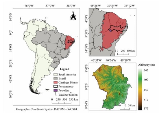
Figure 1.
Spatial location of the study area, municipality of Petrolina, Pernambuco, Northeast Brazil.
A characteristic of the Caatinga biome is the presence of different floristic mosaics, consisting of an area of tree and shrub vegetation, which presents its distribution conditioned to climatic and environmental variations, especially rainfall intensity and frequency [60], as well as geological configurations and soil properties [5]. The vegetation of this biome presents deciduous species adapted to water deficit conditions and with expressive biomass production in rainy seasons, resulting from the local climatic conditions [40,61]. The canopy cover of the species of the Caatinga biome presents discontinuous characteristics, making possible the soil exposure in dry periods, presence of herbaceous stratum, cactus species, and shrubs [23,61]. It is worth noting that this region presents an expressive modification of the native landscape (Caatinga) in areas of irrigated agricultural cultivation.
According to the Köppen–Geiger climate classification, the region’s climate is of the BSh type, characterized as semi-arid tropical, with an average air temperature of 26.4 °C, average relative humidity of 62%, and annual rainfall of 520 mm [62,63]. Rainfall pattern is irregular throughout the year, resulting from its geographical location and the Intertropical Convergence Zone (ITCZ) influence, with rainfall predominating from February to May [10,64,65]. The predominant soils in the municipality are Typic Quartzipsamment, Ultisol Plinthic, Arenosol, and Haplic Acrisol [66,67,68].
2.2. Satellite Images and Weather Datasets
Annual records of average air temperature (°C), global radiation (MJ m−2), relative humidity (%), atmospheric pressure (kPa), wind speed (m s−1), and rainfall (mm) were obtained from the database of the National Institute of Meteorology [69] (Figure 2). The average air temperature (Ta) ranged between 24.1 and 30.7 °C, in which 2015 and 2019 were the warmest years studied (Ta 28 °C). Overall, November, December, January, February, and March presented Ta values above 28 °C (Figure 2).
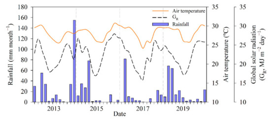
Figure 2.
Monthly meteorological variations (rainfall, average air temperature, and global solar radiation) of the municipality of Petrolina, Brazil, from 2013 to 2019.
The years 2013 (334.4 mm) and 2019 (221.6 mm) showed the highest rainfall rates. Most of the rainfall recorded for Petrolina was concentrated from December to March (Figure 2). Such climatic conditions concerning the municipality were also reported in the literature (e.g., [2,70]).
Rainfall data corresponding to the 30 days prior to the four imaging dates studied used were obtained from the Climate Hazards Group InfraRed Precipitation with Station (CHIRPS). CHIRPS are new precipitation products covering the coordinates 50°S–50°N and 180°E–180°W, with 0.05° (±5.3 km) spatial resolution and daily to seasonal, temporal resolutions, available worldwide since 1981 [71]. CHIRPS data were extracted from the Google Earth Engine platform (https://earthengine.google.com/, accessed on 20 August 2021) using JavaScript programming language. Then, they were exported in spreadsheet format (*.xls), using the dataset since 1981 from the collection ee.ImageCollection (“UCSB-CHG/CHIRPS/DAILY”).
We used Operational Land Imager (OLI) Collection 1 Level 1 bands 2 (0.450–0.51 µm), 3 (0.53–0.59 µm), and 4 (0.64–0.67 µm) in the visible spectrum, 5 (0.85–0.88 µm) in the near-infrared, and 6 (1.57–1.65 µm) and 7 (2.11–2.29 µm) in the shortwave infrared, all with a spatial resolution of 30 m, as well as band 10 from the Thermal Infrared Sensor (TIRS) with a 100 m spatial resolution. Besides this, we used four Landsat-8 OLI/TIRS images, path 217 and row 66, corresponding to the years 2013, 2015, 2017, and 2019 (for the dates and times of the satellite overpass, see Table 1). The choice criteria adopted were the absence of clouds (10%) and the images corresponding to the transition period between the dry and rainy seasons in the region under study, from the years of 2013 to 2019. This period presented severe and extreme drought events in the northeast [23,72]. All the images were obtained from the United States Geological Survey (USGS) platform (https://earthexplorer.usgs.gov/, accessed on 10 August 2021) and processed through the Land Surface Reflectance Code (LaSRC).

Table 1.
Date of the Landsat-8 satellite pass, followed by the Julian day (JD), Earth–Sun distance (dr, astronomical units—AU), local time of the equator pass (h, hour; min, minutes), zenith angle (θ, °), solar elevation angle (E, °), and sun azimuth angle (φ, °) for the municipality of Petrolina, Pernambuco, Brazil.
2.3. Vegetation Indices
The Normalized Difference Vegetation Index (NDVI) was calculated to represent the amount and quality of vegetation present on the surface, characterized as an indicator of wet conditions, calculated using Equation (1).
where ρNIR and ρRed are the reflectances measured in the near-infrared and red bands (i.e., Landsat-8 multispectral bands 5 and 4 of the OLI sensor), respectively, they range from −1 to +1. Values close to 1 on a positive scale correspond to high photosynthetic activity, and when negative, generally correspond to water bodies.
Based on the NDVI, we calculated the vegetation cover (VC) of the study area (Equation (2)), according to Gao et al. [54].
where VC is the vegetation cover, NDVIS is the minimum NDVI value from bare soil pixels obtained in the study area, and NDVIV is the maximum NDVI value found in vegetated areas, i.e., from fully vegetated pixels. The NDVIS and NDVIV used to calculate VC were obtained from the domain of each NDVI image percentile map obtained from the NDVI histograms.
Soil-Adjusted Vegetation Index (SAVI) was calculated to observe the vegetation cover of the area (Equation (3)).
where L is the adjustment factor to the soil, which varies between 0 and 1. The value 0 does not reach change, and resembles the NDVI. In areas with low-density vegetation, the value 1 is assigned; for intermediate-density vegetation areas, the value of 0.5; and for areas with high-density vegetation, the value 0.25 is assigned [74]. The adjustment factor of 0.5 was adopted due to the study region indicating an intermediate vegetation coverage in most of the year, with predominant vegetation of the Caatinga biome, in the Brazilian semi-arid region [75,76,77].
To evaluate changes in vegetation biomass, the leaf area index (LAI, m2 m−2) was determined (Equation (4)), a fundamental biophysical variable for monitoring studies of agricultural land and vegetation moisture conditions [50].
2.4. Methodology for Estimating Evapotranspiration Using Satellite Images
Evapotranspiration was estimated using the Energy Balance Algorithm for Land (SEBAL). For this, routine meteorological data and spectral bands from the Landsat-8 satellite were used. The SEBAL algorithm was implemented using JavaScript code through the Google Earth Engine (GEE) platform. The data were exported in spreadsheet format (*.xls). SEBAL uses mathematical modeling and operations to calculate the surface energy balance components and determine evapotranspiration. Thus, energy balance components are computed pixel-by-pixel, as described in Figure 3. Here, we show that the algorithm has a good performance and high accuracy, as well as being calibrated and validated with simultaneous field and Landsat satellite measurements [47,48,49,56,59,61,78,79].
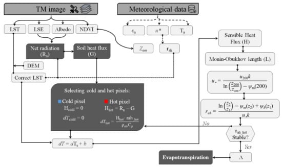
Figure 3.
Flowchart of the SEBAL model for estimating evapotranspiration. Note: LST and LSE are the land surface temperature and land surface emissivity, respectively, NDVI is the Normalized Difference Vegetation Index, εa is the atmospheric emissivity, u* is the friction velocity, Ta is the air temperature, Rn is the net radiation, G is the soil heat flux, zom is the momentum roughness length, z1 and z2 are the two heights between the surface of the anchor pixels, rah is the near-surface aerodynamic resistance to heat transport, DEM is the digital elevation model, dT is the near-surface air temperature gradient, a and b are the calibration coefficients, LST or Ts is the land surface temperature, ρair is the air density, Cp is the specific heat of air, H is the sensible heat flux, ψm and ψh are the stability correction factors for momentum and sensible heat, respectively, k is the von Karman constant, u200 is the wind speed at the height of 200 m, and Λ is the evaporative fraction. These pre- and processing steps were performed inside Google Earth Engine (GEE) cloud platform. The acronyms and symbols used in this study are summarized in the Abbreviations section.
Surface Albedo Adjustment
The surface albedo (αsup) corresponds to a measure of the reflectivity of the Earth’s surface, for each pixel, with atmospheric correction obtained according to Equation (5) [50,80].
where αtoa is the albedo at the top of the atmosphere, that is, before atmospheric correction, αpath is the atmospheric reflectance (set to 0.03, as used by Silva et al. [80]), and τsw is the atmospheric transmissivity for clear sky conditions, according to Equation (6) [50,80]:
where Pa is the atmospheric pressure (kPa), with dataset available freely in https://portal.inmet.gov.br/ (accessed on 10 August 2021), Kt is the turbidity coefficient of the atmosphere (Kt = 1.0, for a clear sky day), according to Allen et al. [47] and Silva et al. [80], θ is the solar zenith angle, and W is the precipitable water (mm), estimated from Equation (7) [81].
where ea is the actual atmospheric water vapor pressure (kPa), estimated from Equation (8).
where HR is the instantaneous relative humidity (%), and es is the water vapor saturation pressure (kPa), estimated from Equation (9).
where T0 is the instantaneous air temperature (°C) at the moment of the satellite pass.
For obtaining αtoa, a linear combination of the spectral reflectance of the six reflective OLI bands was performed according to Equation (10) [80]:
where r2, r3, r4, r5, r6, and r7 are the surface spectral reflectances for bands 2, 3, 4, 5, 6, and 7 of the Landsat-8 OLI, respectively.
We use Equation (11) to obtain each of the spectral reflectances.
where the terms Addb and Multb belong to the radiometric rescaling group, specifically reflectance_add_band (equal to −0.1) and reflectance_mult_band (equal to 0.00002), respectively, presented in the metadata of each OLI—Landsat-8 image, DN is the digital number value corresponding to the pixel, θ is the solar zenith angle at the data acquisition time, and dr is the Earth–Sun distance in astronomical units.
2.5. Determination of Surface-energy Partitioning
Based on the surface energy balance components, the evaporative fraction was determined. Initially, the surface radiation balance or net radiation—Rn was calculated, which is distributed by the energy partitioning in front of the sensible heat fluxes—H, latent—LE, and soil heat flux—G [47,48,49,50,61,78,79]. By performing this process, a linear relationship between the surface and air temperature gradient was considered to exist. From this relationship and the internal calibration process for extreme conditions such as temperature and humidity, it was established the need for obtaining the knowledge of the so-called “anchor pixels”, i.e., hot and cold pixels, which are indicative of zero and maximum evapotranspiration, respectively [47,48,61] (Figure 3).
The land surface temperature (LST) in K (Kelvin) was obtained using the spectral radiance in band 10 of the TIRS sensor and the emissivity in the nearest band—εnb by the modified Planck’s Law [82], as described in Equation (12).
where K1 and K2 are radiation constants specific for the Landsat-8 TIRS band 10, equaling 774.89 W m−2 sr−1 μm−1 and 1321.08 K, respectively, provided by NASA/USGS; and L10 is the radiance at the wavelength received by the sensors (band 10, the thermal band).
The εnb was calculated based on the LAI for each pixel according to Equation (13) [41].
Initially, the temperature variation and aerodynamic resistance to heat transport in all pixels of the study area (Petrolina, Pernambuco) were determined. The atmosphere was initially assumed to be in a neutral stability condition. For this study, the hot pixel was considered in the exposed soil plots (i.e., no vegetation cover and/or little vegetation and low moisture content), assuming LE equal to zero. The cold pixel was considered in grape orchard plots irrigated by micro-sprinklers, when H can be considered zero [47,48,61,78,79,83] (see Figure 3). Since turbulent effects affect atmospheric conditions and air resistance, the Monin–Obukhov similarity theory was applied and considered in the computation of H in all pixels of the study area. It is worth noting that the Monin–Obukhov length was used for corrections to the initial stable condition of the atmosphere [47,48,49,78,79].
Calculation of Energy Fluxes (H and LE) and Evaporative Fraction
The sensible heat flux (H) in SEBAL is calculated using an iterative procedure from the aerodynamic function (Equation (14)) [47,48,49,78,79].
where ρair is the moist air density (kg m−3), Cp is the air specific heat at constant pressure (1004 J kg−1 K−1), a and b are calibration constants of the temperature difference between two heights (i.e., between the roughness length for heat transfer and the reference height, usually 0.1 and 2.0 m above the displacement plane), and rah is the near-surface aerodynamic resistance to heat transport (s m−1). Fundamentally, the coefficients a and b are determined through an internal calibration for each satellite image by interactive processes. We consider extreme pixels of wet/cold and dry/hot spots. They were selected to develop a linear relationship between the aerodynamic temperature of the surface and the air temperature difference, and the LST.
By knowing the components of the surface energy balance, such as the net radiation (Rn, W m−2), sensible heat flux (H, W m−2), and soil heat flux (G, W m−2), the latent heat flux (LE, W m−2) was determined, both corresponding to the time of the satellite pass over the study area, according to Equation (15).
Subsequently, we determined the evaporative fraction (Λ) according to Equation (16).
2.6. Estimate of ETa Using SEBAL Method
Finally, as a SEBAL product, we determine the actual evapotranspiration (ETa, mm day−1) [84] based on Equation (17) below, for each satellite image used. In this study, the implemented SEBAL model had already been extensively validated and calibrated under forests and agricultural land conditions [56,61,85].
where Rn24 is the daily net radiation (W m−2), 86,400 is a constant for daily timescale conversion (i.e., converts from seconds to days), and λ is the latent heat of vaporization of water (J kg−1). Then, the latent heat of vaporization allows the ETa expression in mm day−1. Hence, accurate estimation of Rn24 (Equation (18)) was determined according to Bastiaanssen et al. [49], and Lee and Kim [86]:
where a is a regression coefficient of the relationship between net longwave radiation and atmospheric transmissivity on a daily scale, to which we assigned the value 143, as proposed by Teixeira et al. [61]. The acronyms and symbols used in this study are summarized in the Abbreviations section.
2.7. Land Use and Land Cover Dynamics
In the present study, we sought to evaluate the impacts of changes in land use and land cover (LULC) under the biophysical variables in the municipality of Petrolina. Thus, we performed the extraction of descriptive statistical parameters (i.e., minimum, maximum, mean, median, and standard deviation) for the variables LAI, VC, ETa, LE, H, LST, emissivity, and Rn in each class of LULC, from the maps available on the MapBiomas Brazil platform [87]. This collection is highly reliable and it includes annual land use and land cover (LULC) data for the period 1985–2019 and it prioritizes the following classes: (1) arboreal Caatinga, (2) shrub Caatinga, (3) herbaceous Caatinga, (4) pasture, (5) agriculture, (6) mosaic of agriculture and pasture, (7) urban area, and (8) water bodies with a spatial resolution of 30 meters [27,88].
The MapBiomas classification is a hierarchical system combining land use and land cover. This classification is based on a pixel-by-pixel classification of Landsat images, where we use the machine learning algorithm random forest. Thus, the LULC classes for 2013, 2015, 2017, and 2019 were converted from raster files to vector files. We use the “polygonise” tool, which transforms classes into polygons with the help of QGIS 3.16 software [89]. After the new datasets were converted, the vector files were used to extract the statistical parameters by using the “zonal statistics” tool of the QGIS 3.16 software [89]. This procedure provided a basis with greater data amplitude and greater coverage of the region’s surface under study, making it possible to compare the different land use and land cover types. In addition, as a result of this process, four maps were generated, indicating the land use and land cover changes.
2.8. Statistical Analyses
In this study, we applied a principal component analysis (PCA) on the biophysical variables—e.g., LAI, VC, ETa, LE, H, LST, albedo, emissivity, and Rn—for 2013, 2015, 2017, and 2019. Principal component analysis was performed to reduce the large dataset and convert the data series into sets of uncorrelated linear values without losing relevant information [35,65]. PCA consists of computing the eigenvalues and eigenvectors of the covariance matrix. Moreover, in the generation of PCA, diverse components are created, and the first component is the most important, as it explains the highest percentage of the data variance, while the later components created in the analysis represent a lower variation of the data. Thus, the data were standardized, subtracting the minimum values from each value and dividing by their interval in order to obtain the maximum amount of information extracted. Only eigenvalues greater than 1.0 were taken into account, for they present expressive information from the newly created dataset [90]. The generated loadings indicate the relative importance of a given raw variable from the data sample in the principal component (PC) [65]. Moreover, 400 random points were generated to compose the data of our regression model. One hundred random points were generated across the study area (for variables LST, H, and ETa using SEBAL) for each assessment date [2] through the QGIS (e.g., using the “random points inside polygon” and “point sampling” functions [89]).
Subsequently, we built a multiple linear regression model to determine ETa (predictand) in a simplified way. The selected variables were LST and H (predictors) due to their strong correlation over the years with land use and land cover classes (results obtained using PCA). This type of regression model assumes that there is a linear relationship between the response variable y and the predictor variables (e.g., x1, x2, …, xn); it may be described as follows: y = β0 + β1x1 + β2x2 + … + βnxn + εrr, wherein β0 is the constant value, β1, …, βn are regression coefficients, and εrr is the random error. The threshold for predictor variable inclusion was p < 0.05.
Goodness of Fit
The model performance analysis was based on the root mean square error (RMSE, the values close to zero reduce error and increase accuracy), the mean absolute error (MAE), percent bias (PBIAS), Nash–Sutcliffe efficiency coefficient (NSE), Lin’s concordance correlation coefficient (LCCC), Willmott’s index of agreement (d), which ranges from 0 to 1 (i.e., indicates no agreement at all and perfect agreement, respectively) [91,92,93,94], and coefficient of determination (R2, i.e., indicates the model’s accuracy in the prediction of response for a dataset) above 0.90. These metrics allowed us to evaluate the models’ quality and enabled the extraction of relevant information in terms of applicability. Therefore, the lower the PBIAS and RMSE values, the better the model prediction performance. Furthermore, NSE is a reliable criterion for evaluating the model’s predictive ability. We also used LCCC to measure precision and accuracy between predicted and measured values. Moreover, it indicates the degree of agreement between two methods by measuring the variation of their linear relationship from the 45-degree line through the origin. Thus, good models have LCCC equal or close to 1 [92,93,94]. Additionally, we applied analysis of variance (ANOVA) and the F-test (p < 0.05, Fisher’s F-test) to investigate the statistical significance between ETa values measured by the SEBAL algorithm and predicted by the model proposed in this study. All statistical analyses were performed using the R software [95].
3. Results and Discussion
3.1. Comparisons of Land Use and Land Cover (LULC)
Based on the classification via the MapBiomas platform and on the Landsat-8 satellite, the thematic maps of land use and land cover for the years 2013, 2015, 2017, and 2019 were highlighted, with the main classes represented in Figure 4.
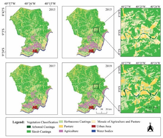
Figure 4.
Thematic classification of cover and land use and occupation from MapBiomas between the years 2013 and 2019 for Petrolina, Pernambuco, Brazil.
The advances in exploration of agricultural areas for the municipality of Petrolina occurred mainly in areas nearby the São Francisco river, with a predominance of irrigated fruit farming. Moreover, the irrigated perimeters “Senador Nilo Coelho” and “Bebedouro” in these areas are located there, which, in the 1970s with the construction of the Sobradinho dam, boosted the exploitation and change in land use, impacting the Caatinga [37,96].
In 2013, 70.20% of the area (320,265.44 ha) of Petrolina was composed of Caatinga, being 51.60% shrub, 18.48% herbaceous, and the other 0.12% arboreal (see Figure 4 and Table 2).
Table 2.
Annual quantification of land use and land cover conditions from 2013 to 2019 for the semi-arid region of Petrolina, Pernambuco, Brazil.
The lowest percentages of areas occupied by Caatinga vegetation were observed in 2015 (67.8%) and 2017 (68.7%), respectively. Compared to 2013, there was an average reduction of 2%, equivalent to 9123.65 ha of native forest (Caatinga), while in 2019, the reduction was only 0.45% (Table 2). It is important to emphasize that the reduction in Caatinga refers to herbaceous native vegetation. Such phenomena are related to the increase in areas of agriculture, pasture, and urban infrastructure, along with the occurrence of lower rainfall rates recorded between 2015 and 2017. However, between 2013 and 2019, an increase of 0.07 and 0.66% was observed in the native trees and shrubs vegetation areas, respectively (Figure 4 and Table 2). Furthermore, the expansion of arboreal vegetation areas occurred close to water bodies; on the other hand, the expansion of shrub vegetation occurred to replace areas previously occupied by agricultural activities (3234.56 ha), mainly pasture or in the ecological succession of areas of herbaceous vegetation (3679.17 ha) (Supplementary Table S1 and Figure S1). Silva et al. [97] studied the spatial–temporal evolution of agricultural activity in the Brazilian semi-arid region from 1998 to 2018, seeking to investigate the resilience of the Caatinga biome during the dry season. The authors mention that the expansion of the Caatinga biome occurred mainly with the reduction of agricultural activity, which reinforces the results obtained in the present study.
In 2013, the areas occupied with pasture represented 11.7%, agriculture 7.0%, and the mosaic of agriculture and pasture 8.64%, while areas with urban infrastructure and water bodies presented an occupation of 1.06 and 1.40%, respectively (Figure 4 and Table 2). From 2013 to 2019, there was an increase in areas with agricultural activity in the region, while a decrease in native herbaceous vegetation (Caatinga) was observed, which caused the conversion of 10,972.34 ha of native herbaceous vegetation to areas of agricultural activity (see Supplementary Table S1 and Figure S1). The types of LULC indicated the different intensities of human activities in the area. Several authors have reported the occurrence of severe drought events in NEB in the period between 2012 to 2016, in addition to the intensification of anthropic activities in the study region [10,23,27,72,98,99]. Those factors are responsible for significant changes in the phytosociology and floristic composition of the biome [10,23,27,72,98,99].
Drought is costly to Brazil, for it causes strong impacts on agriculture and cattle ranching. For example, the 2012–2013 drought resulted in economic losses of USD 1.5 billion for more than ten important crops in the region and USD 1.6 billion in cattle mortality [100]. Furthermore, Marengo et al. [10] emphasize that among adverse natural climate phenomena, drought is the factor that most affects society, as it impacts large territorial extensions of NEB, with intensified and increasingly long-lasting events over the years.
The agricultural and cattle ranching activity were significant in 2015, 2017, and 2019 with 29.6, 28.7, and 27.7%, respectively. Among the agricultural activities, the class of pastures (in this study, there is no detailed distinction between irrigated and non-irrigated pasture areas) was responsible for the largest occupied area, with values of 55,356 ha in 2015; 60,156 ha in 2017, and 60,176 ha in 2019 (see Table 2). The expansion of pasture areas resulted from the growing demand for food and for animal production, which favored changes in land use and occupation and, consequently, it increased the deforestation rate of the Caatinga biome [19]. Fleischer et al. [101] reported that the constant changes in land use and land cover might cause a significant impact on the flux and carbon stock since they are responsible for changing the sink capacity or carbon source of the ecosystem.
The agriculture class in 2015, 2017, and 2019 showed territorial occupation of 34,209, 35,678, and 36,718 ha, respectively, with an average increase of 0.80% (3616 ha) compared to 2013 (Table 2). This growth was favored by the development of irrigated agriculture in the region, due to the proximity of the São Francisco river’s channel, maximizing mainly fruit farming, e.g., grape and mango [6,7]. Most of the times, irrigated fields are inserted in areas previously occupied by Caatinga, which results in changes in the physical, chemical, and biological soil properties [6,66]. In addition, changes in greenhouse gas (GHG) emission fluxes resulting from anthropogenic modifications on native vegetation are also reported in the literature [19,101].
3.2. Rainfall Variability in Land Cover Classes
Analyzing the spatiotemporal rainfall dynamics in the region over the 30 days preceding the passage of the Landsat-8 satellite on the four assessment dates (5 October 2013, 12 November 2015, 16 October 2017, and 7 November 2019) allowed us to observe the variation in rainfall distribution and volume, whose average accumulated values were 5.63, 1.7, 0.59, and 10.4 mm, for the respective dates. Despite the low rainfall volume observed in the region, some areas showed a tendency for higher rainfall occurrence, which may be conditioned to the native vegetation and orographic effects of the region (Figure 5).
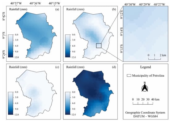
Figure 5.
Spatiotemporal rainfall distribution (mm) for the CHIRPS satellite product in the municipality of Petrolina, Pernambuco, Brazil, in the 30-day period before the imaging dates 5 October 2013 (a), 12 November 2015 (b), 16 October 2017 (c), and 7 November 2019 (d).
Variations in rainfall distributions and volumes may have caused changes in vegetation cover, surface temperature, and evapotranspiration of the land portions observed in this study. Predominant vegetation of the Caatinga biome is quickly responsive to rainfall regimes, reducing foliage in the dry period (through deciduousness) and gaining biomass by the arrival of a new rainy period, which is considered a condition of defense and physiological adaptation of these highly efficient plants [102,103].
3.3. Vegetation Cover Indices of the Municipality
Figure 6 shows the percent vegetation cover (VC) in Petrolina. The first three imaging dates in the study showed that, on average, 52.26% of the territorial area of the region had 0 to 25% vegetation cover (Figure 6a–c), revealing the direct effects of low rainfall volumes resulting from the dry season on native vegetation.
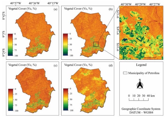
Figure 6.
Condition of the different types of vegetation cover in the Caatinga agroecosystem in the municipality of Petrolina, Pernambuco, Brazil, on the imaging dates 5 October 2013 (a), 12 November 2015 (b), 16 October 2017 (c) and 7 November 2019 (d).
Under these conditions, variations in NDVI values are strongly linked to biomass production [102]. In studies carried out in the Caatinga, Cunha et al. [22], Leivas et al. [21], and Leivas et al. [104] reported that monitoring large-scale variations of water indicators and vegetation status is of crucial importance to minimize the adverse effects of climate and land use changes on mixed agroecosystems. Moreover, it can help in planning and decision-making processes for rational use of natural resources to mitigate the effects and duration of large-scale drought events.
The results reported here contribute to understanding water limitations and vegetation behavior. Due to the proximity of the São Francisco river, which supplies the irrigation systems, the areas of higher vegetation cover are found in the irrigated agriculture sites in the southern part of the municipality and the few remaining fragments of arboreal Caatinga, reaching average values of 58.71 ± 22.18% and 59.78 ± 18.94%, respectively, throughout the period under study (Figure 6). However, it can be observed that in areas dominated by pasture, herbaceous, and shrub Caatinga, the mean values of VC for the dates studied are lower (22.84 ± 6.70%, 27.17 ± 5.45%, and 24.56 ± 4.74%, respectively) (see also Figure 4). The advanced stage of pasture degradation and the intense grazing activity in natural areas of Caatinga also impact the vegetation density and, hence, its spatiotemporal dynamics and related surface variables such as NDVI, LST, albedo, and emissivity [2,72,105].
Santos et al. [103] emphasize that the arboreal vegetation is less susceptible to climatic variations than shrub and herbaceous vegetation, leading to less drastic reductions in VC throughout the dry season. This characteristic is intrinsically linked to the adaptive capacity of species, favoring them to withstand the stressful effects of abiotic factors [106].
It is essential to highlight that on 7 November 2019, there was an average increase of 46.81% of areas with VC higher than 50% in the northern part of the municipality (Figure 6d), which indicates a response of vegetation to the behavior of rainfall in this period, since this was the fraction of the polygon with the highest rainfall index during the 30 days prior to this evaluation date (Figure 5 and Figure 6). The interrelationship of vegetation with meteorological variables plays a crucial role in the ability to slow the advance of aridity, loss of soil quality, and ecological diversity. In areas with consolidated vegetation, soil exposure to solar radiation becomes lower, causing the maintenance of soil moisture and consequently favoring the water availability in the environment for species. The intensification of anthropic activities can directly cause damage to native vegetation, such as soil and vegetation degradation; however, these changes can also influence climatic conditions and cause severe damage to ecosystem services.
During the studied dates, the LAI varied between 0.00 and 3.3 m2 m−2 (Figure 7). However, in 97% of the region under study, the LAI values were lower than 0.825 m2 m−2, for in periods with low water availability, the Caatinga usually presents low LAI [107]. The low LAI values can be justified not only by drought events but also by the characteristics of the soils, which, in general, are shallow and have low water storage capacity. In addition, it is worth noting that factors such as deforestation and intensive grazing activity in areas of native vegetation, as well as a high degree of degradation of pasture areas, historically, are common in this region, causing an imbalance of natural ecosystems [108,109].
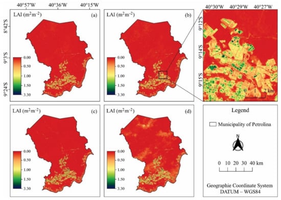
Figure 7.
Spatiotemporal distribution of leaf area index (LAI, m2 m−2) in the municipality of Petrolina, Pernambuco, Brazil, on the imaging dates 5 October 2013 (a), 12 November 2015 (b), 16 October 2017 (c), and 7 November 2019 (d).
The highest heterogeneity in LAI values was seen on 7 November 2019 (0.24 ± 0.22 m2 m−2) (Figure 7d), increasing from the greater variability in the spatial distribution of rainfall accumulation in the previous days. On the other hand, during the dates studied here, the highest mean LAI values stood out only in areas of arboreal Caatinga (0.58 ± 0.45 m2 m−2) and agriculture (0.75 ± 0.49 m2 m−2), with the maximum values being associated with irrigated agricultural areas, more specifically orchards, with increased biomass production. However, in areas of pasture, urban infrastructure, and areas of arboreal and herbaceous Caatinga, the LAI values were close to or equal to zero, making its variation more homogeneous, that is, closer to the daily mean, with standard deviation (SD) ranging between 0.05 and 0.10 m2 m−2 within the land cover classes (Figure 7).
3.4. Land Surface Temperature (LST) in the Studied Classes
In the present study, the minimum LST values were seen in areas of water bodies, while the maximum LST values were seen in areas of exposed soils, located at points of pasture and degraded Caatinga, urban infrastructure (asphalt, concrete, and gravel surfaces), and agricultural areas undergoing soil preparation for cultivation (Figure 8). This result is expected in bare soil locations under intense anthropic activity due to the transformation of land use/land cover classes into non-evaporating surfaces. This makes the place’s temperature higher and reduces water availability in the soil, which causes serious problems in agricultural crops. The computed LST map is shown in Figure 8.
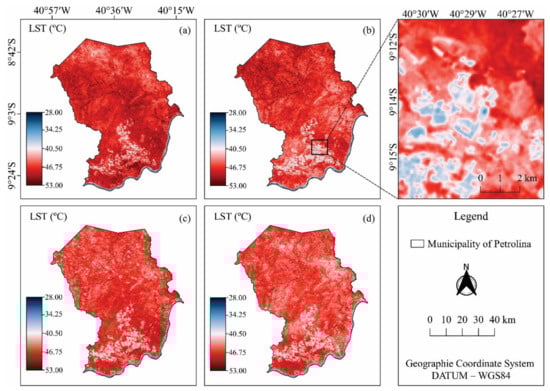
Figure 8.
Spatiotemporal distribution of the land surface temperature—LST (°C) in the municipality of Petrolina, Pernambuco, Brazil, on the imaging dates 5 October 2013 (a), 12 November 2015 (b), 16 October 2017 (c) and 7 November 2019 (d).
Due to the replacement of primary vegetation with pastures, agricultural crops, and urban occupation, changes in land use can substantially affect the heat and mass exchange in the soil–plant–atmosphere system, propitiating the retention of a higher amount of heat by the Earth’s surface [2,52]. Land abandonment and excessive mechanical disturbance of the soil may also alter the heat exchange with the environment and cause lower thermal and radiant energy lag; thus, the land conversion had increased LST in the area of the non-evaporating surfaces.
It can be observed that the average LST values for the dates studied were higher in the areas dominated by pasture (47.69 ± 1.47 °C), herbaceous Caatinga (47.28 ± 1.27 °C), and shrub Caatinga (46.07 ± 1.44 °C), even higher than those observed in areas with urban infrastructure (45.80 ± 1.52 °C) (Figure 8). According to Zhao et al. [110,111], sites with different land cover types may have an LST increase gradient along the urban to rural profile. The high LST in the pasture, herbaceous, and shrub Caatinga areas is related to the lower percentage of ground covering by vegetation (see Figure 6), which results in drier exposed soil, with higher albedos and lower evaporative cooling flux rates, a factor that increases LST. Another related factor contributing to the high LST of pastures is that grasses have shallower roots. Therefore, they can only access the water available in the superficial soil layers, which depletes faster than in deeper layers [2]. Vegetation canopy can retain rainwater and decrease groundwater recharge by altering evaporative flux and raising the land surface temperature.
On the other hand, it is observed, in general, that in areas dominated by arboreal Caatinga and agriculture, the average LST values are lower (38.99 ± 2.48 °C and 43.11 ± 2.30 °C, respectively) (Figure 8). The highest vegetation cover and the highest soil humidity in the areas dominated by these classes favor LST reduction. However, they present the greatest spatial variations of LST among all land use and land cover classes, according to the standard deviation values (±SD). The main advantage of using LST data from satellite images is the total surface coverage. In this way, each time series of pixels of the LST map can be considered a “virtual weather station” [112].
3.5. Variations of the Actual Evapotranspiration (ETa) of Land Use Classes
Rainfall regime directly influenced ETa, so that on 16 October 2017 (Figure 9c), the date with the lowest rainfall accumulation in the previous days, the lowest ETa rates were found, with an average value of 2.02 mm day−1. On the other hand, on 7 November 2019 (Figure 9d), the period with the highest rainfall accumulation, average ETa rates were 2.62 mm day−1 (Figure 9). According to Teixeira et al. [20], high evapotranspiration values in Caatinga areas occur right after rains. Therefore, the previous rainfall raises soil water availability and keeps native species with turgid structures and greener canopy.
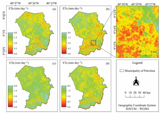
Figure 9.
Spatiotemporal distribution of actual evapotranspiration (ETa, mm day−1), calculated with Surface Energy Balance Algorithm for Land (SEBAL), in the municipality of Petrolina, Pernambuco, Brazil, on the imaging dates 5 October 2013 (a), 12 November 2015 (b), 16 October 2017 (c), and 7 November 2019 (d).
The ETa estimated by the SEBAL model showed variation both within and between land use and land cover classes. The lowest ETa observations in all the evaluated dates were observed in the areas occupied by pasture and mosaic of agriculture and pasture classes, with average values of 0.70 ± 0.73 mm day−1 and 1.01 ± 0.96 mm day−1, respectively (Figure 9). These areas have dryland cultivation practices, which causes the lower water availability to affect the evapotranspiration rates; moreover, the heterogeneity of the areas causes sudden variations in ETa.
On the other hand, due to the effect of the increase in air temperature and atmospheric demand verified throughout the dry season in Petrolina, combined with the presence of preserved riparian forests along stretches of water bodies and continuous irrigation in crops, higher mean ETa values were observed in the arboreal Caatinga (4.73 ± 0.49 mm day−1) and agriculture (3.07 ± 1.23 mm day−1) classes. For presenting areas with irrigated and dry cultivation, the average values of this class become more variable. When there is a greater contribution of moisture added to more dense vegetation, there is a favoring of the local microclimate in the region [113,114], a phenomenon reported in areas of arboreal vegetation.
The shrub and herbaceous Caatinga classes showed greater heterogeneity indicated by the largest standard deviations (2.42 ± 0.76 mm day−1) and (1.46 ± 0.71 mm day−1), respectively, relative to the arboreal Caatinga class (Figure 9). Folhes et al. [115] reported that the evapotranspiration values (2.0 mm day−1) during the dry season for species of herbaceous–shrubby Caatinga. In dry periods, the Caatinga vegetation uses the available energy as sensible heat flux (H), limiting transpiration and photosynthesis, thus reducing evapotranspiration values [20]. However, arboreal vegetation is able to compensate the high vapor pressure deficit in the air, even in dry periods, when compared to shrub and herbaceous vegetation, due to the deep root system keeping up with the water stored in the soil [70,116,117].
The arboreal and shrub species play a fundamental eco-hydrological role, maintaining soil humidity and structuring its porosity, guaranteeing the maintenance of infiltration capacity and favoring the survival of species [116].
3.6. Statistical Relations between the Variables Studied and Land Use
In this study, we performed a PCA of the environmental variables in relation to land use and land cover classes. Therefore, the first two components with eigenvalues greater than 1.0 were extracted separately for the years 2013, 2015, 2017, and 2019 (Figure 10). In 2013, the two principal components explained 94.77% of the total variation, with 70.39% in the principal component 1 (PC1) and 24.38% in the principal component 2 (PC2). On the other hand, in 2015, 2017, and 2019, when added together, PC1 and PC2 represented 94.01, 92.34, and 94.56% of the total variation, respectively (Figure 10). In addition, it can be seen that the LULC class, with the least influence on components 1 and 2 in all years, is shrub Caatinga, with average eigenvalues (0.31 and 0.37, respectively). In addition, the classes with the greatest influence on PC1 with positive and negative eigenvalues are water bodies (2.69), agriculture (−2.35), arboreal Caatinga (−1.92), pasture (0.34), mosaic (0.16), and urban area (0.35). In PC2, the classes of LULC were water bodies (−4.36), mosaic (2.10), agriculture (−1.0), and arboreal Caatinga (−3.40) (Figure 10).
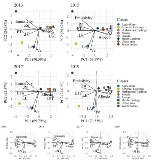
Figure 10.
Scores obtained by principal component analysis (PCA) of environmental variables and land use and land cover. PC1 and PC2 are the first and second dimensions of PCA data, respectively. The four inserted panels below the PCA scores plots refer to the loadings plots of the first two principal components from 2013 to 2019.
Through PCA, we observed that the ordering of variables in each principal component (PC) of the axes was influenced by the degree of vegetation cover and surface water status of the LULC classes (Figure 10). Thus, PC1 contributed more to the variability of the response of variables related to energy balance. Therefore, in PC2, the land use and land cover classes (i.e., pasture, mosaic, urban area, and herbaceous Caatinga) influenced the variables Rn, LE, ETa, and emissivity with higher mean loadings (−0.95, −0.94, −0.99, and −0.80, respectively). On the other hand, they showed a high correlation with the variables H, LST, and albedo. For these LULC classes, this may be related to the presence of bare soil and thin vegetation covers that affect the regional microclimate and soil–plant–atmosphere system fluxes, resulting in higher albedos, lower rates of evaporative cooling fluxes, and highest LST [2,105].
On the other hand, PC2 contributed more to the variability of the responses of the variables regarding the canopy interactions (LAI and VC) due to the strong negative correlation with cultivated land (i.e., agriculture class) (Figure 10). In all years, there was a predominance for LE and LAI in areas with arboreal Caatinga and agriculture, with agriculture presenting the highest VC. Caatinga presents a strong relationship with LAI in rainy periods due to the greater availability of water in the soil [118]. In the present study, the samples were taken in the period with low rainfall, so the LAI was not expressive compared to agricultural areas, which use irrigation and therefore increase the LAI. Thus, the emissivity in the Caatinga vegetation is lower, for the emissivity of the soil is generally lower than that of the leaves [2].
The results of the analysis of variance (ANOVA) and multiple regression analysis of the established model are presented in Table 3. For the combination of two-variable models, the two best pre-established parameters based on the PCA results were the variables LST and H, used to build the regression model. In particular, these two variables are of great relevance in transferring energy to the atmosphere. The ANOVA results also showed that the model values are significant. Due to the observations, a joint analysis of the coefficient of determination obtained (R2 = 0.98) can be performed, emphasizing the P-value obtained from our regression model, which was less than 0.001, thus indicating greater model accuracy and reliability (Table 3). Notably, it can be seen that the model’s F-value was 16,692.84, being greater than the critical value of F0.05 = 3.018, which confirms the significance of the proposed model. In addition, the variables used provided a high R2 and LCCC, being essential for the model’s accuracy. Furthermore, the results showed that the multiple linear regression model to determine ETa achieved a coefficient of determination of 0.98, RMSE of 0.498, MAE of 0.413, and d equal to 0.9620. It also resulted in PBIAS, NSE, and LCCC values averaged between −13.32%, 0.826, and 0.907, respectively (Table 3). From the statistical analysis, this model is described as ETa = 6.89 − 0.0527LST − 0.0120H. Based on the RMSE, LCCC, and d of this application, the use of the ETa model, besides presenting a strong correlation between the variables H and LST, as seen in Figure 10, expresses a biophysical model with enough efficiency and high agreement to determine ETa.
Table 3.
Analysis of variance (ANOVA) and regression coefficients results for the suggested model.
The high d (0.9620) values for ETa indicated that there was a good agreement between simulated and measured ETa. In general, the ETa model showed excellent agreement (LCCC 0.9), high performance, and low RMSE (0.498) (Table 3). The PBIAS and MAE values for ETa were between −13.32% and 0.413, confirming the close agreement. Consequently, this result describes the ability to simplify and accurately predict ETa in deficit environments. Applications of regression model analysis with environmental variables are common in the literature in dry forests [118,119,120]. However, these implementations of variables in previous studies may be challenging to acquire for specific locations, requiring more simplified models. Our results also indicate the relationship between H and the LST of ecosystems to determine ETa, an important variable in the energy balances of environments worldwide.
4. Conclusions
In this study, we point out a significant tendency to increase the agricultural areas, which results in the progressive decrease of the Brazilian Caatinga biome. The vegetation cover is directly influenced by the soil–water regime; years of higher rainfall result in a lower percentage of suppression of the native forest in the municipality of Petrolina, Pernambuco (Brazil). The areas with pasture class presented hotspots due to degradative processes and higher surface temperatures, influenced by the sensible heat flux. A gradual increase in LST is observed in the municipality and it may cause future risks to forest areas.
The SEBAL algorithm used in a semi-arid environment is a helpful tool to determine the energy and mass fluxes in different ecosystems. Notably, the Caatinga biome has particularities in biophysical parameters, according to the land cover and soil exposure on intra and inter-annual scales. The heterogeneity of the surface of the municipality of Petrolina, as a function of land use and land cover patterns, alters the energy exchange with the atmosphere. Our results also suggest a simplified and validated model for ETa determination in a semi-arid environment. The regression model could accurately predict the spatial distribution of ETa, with high R2 and LCCC and low RMSE value.
Thus, it is possible to suggest that the implementation of agricultural activities in the Petrolina should be carried out in a planned and sustainable way in order to mitigate the impacts that anthropic action causes on the Caatinga, especially with the increased vulnerability of this biome to the desertification process. However, further research is needed to investigate the spatial variations of the types of crops covering the soil in the municipality, as well as the dynamics of fires and their impacts on the diversity of the Caatinga biome. Field surveys and the use of unmanned aerial systems (UAS) could provide more detailed information at an intermediate and fine scale.
Supplementary Materials
The following are available online at https://www.mdpi.com/article/10.3390/rs14081911/s1, Figure S1: Land use/land cover changes in Petrolina between 2013 and 2019. Positive values indicate an expansion of the respective land cover, negative values a contraction. The vertical axe is in million hectares (Mha). Please see Supplementary Table S1 to access values of land use/land cover changes; Table S1: Areas of expansion and contraction of land use/land cover changes in Petrolina between 2013 and 2019. Positive values indicate an expansion of the respective land cover, negative values a contraction. The values are in million hectares (Mha).
Author Contributions
Conceptualization, A.M.d.R.F.J. and G.d.N.A.J.; methodology, M.V.d.S., A.d.S., and A.M.d.R.F.J.; software, M.V.d.S., A.d.S., and A.M.d.R.F.J.; validation, J.F.d.O.-J. and A.H.d.C.T.; investigation, J.L.B.d.S., H.P., P.E.T., L.S.B.d.S., and C.A.d.S.J.; data curation, M.V.d.S., A.d.S., A.M.d.R.F.J., and G.d.N.A.J.; writing—original draft preparation, A.M.d.R.F.J.; writing—review and editing, T.G.F.d.S., J.L.M.P.d.L., and E.A.S.; visualization, J.L.M.P.d.L. and A.H.d.C.T.; supervision, A.H.d.C.T., T.G.F.d.S., and J.F.d.O.-J.; project administration, T.G.F.d.S. and J.L.M.P.d.L.; funding acquisition, J.L.M.P.d.L. All authors have read and agreed to the published version of the manuscript.
Funding
This research was funded by the Portuguese Foundation for Science and Technology (FCT), through projects ASHMOB (CENTRO-01-0145-FEDER-029351), GOLis (PDR2020-101-030913, Partnership nr. 344/Initiative nr. 21), MUSSELFLOW (PTDC/BIA-EVL/29199/2017), MEDWATERICE (PRIMA/0006/2018), and through the strategic project UIDB/04292/2020 granted to MARE—Marine and Environmental Sciences Centre, University of Coimbra, Coimbra, Portugal.
Institutional Review Board Statement
Not applicable.
Informed Consent Statement
Not applicable.
Data Availability Statement
Landsat-8 image courtesy of the USGS/NASA (https://www.usgs.gov/core-science-systems/nli/landsat, accessed on 10 August 2021); MapBiomas data presented in this study are available at websites of Brazilian Annual Land Use and Land Cover Mapping Project (https://mapbiomas.org/en/project, accessed on 20 August 2021); and the meteorological data presented in this study are available at the website of the National Institute of Meteorology (https://portal.inmet.gov.br/, accessed on 10 August 2021).
Acknowledgments
The authors would like to thank the Research Support Foundation of the Pernambuco State (FACEPE, Brazil—APQ-0215-5.01/10 and FACEPE - APQ-1159-1.07/14), the National Council for Scientific and Technological Development (CNPq, Brazil) and also funds through the fellowship of the Research Productivity Program (CNPq 305286/2015-3, 304060/2016-0, 309681/2019-7, and 303767/2020-0), and the Coordination for the Improvement of Higher Education Personnel (CAPES, Brazil - Finance Code 001) for the research and study grants. The authors are also grateful for financial support from the Portuguese Foundation for Science and Technology (FCT), and the University of Coimbra, Portugal. In addition, we also would like to thank the anonymous reviewers for their insightful comments, of which significantly increased the value of this study.
Conflicts of Interest
The authors declare no conflict of interest.
Abbreviations
Summary of all the symbols and acronyms used in this paper.
| Item | Description |
| a and b | Are the calibration coefficients |
| Cp | Specific heat of air |
| d | Willmott’s index of agreement |
| DEM | Digital elevation model |
| dT | Near-surface air temperature gradient |
| ea | Actual atmospheric water vapor pressure |
| es | Water vapor saturation pressure |
| ETa | Actual evapotranspiration |
| G | Soil heat flux |
| GEE | Google Earth Engine |
| H | Sensible heat flux |
| HR | Instantaneous relative humidity |
| k | von Karman constant |
| LAI | Leaf area index |
| LCCC | Lin’s concordance correlation coefficient |
| LE | Latent heat flux |
| LSE | Land surface emissivity |
| LST | Land surface temperature |
| LULC | Land use and land cover |
| MAE | Mean absolute error |
| NDVI | Normalized Difference Vegetation Index |
| NSE | Nash-Sutcliffe efficiency coefficient |
| PBIAS | Percent bias |
| PCA | Principal component analysis |
| rah | Near-surface aerodynamic resistance to heat transport |
| RMSE | Root mean square error |
| Rn | Net radiation |
| Rn24 | Daily net radiation |
| R2 | Coefficient of determination |
| SAVI | Soil-Adjusted Vegetation Index |
| T0 | Instantaneous air temperature |
| Ta | Air temperature |
| u* | Friction velocity |
| u200 | Wind speed at the height of 200 m |
| VC | Vegetation cover |
| W | Precipitable water |
| z1 and z2 | Are the two heights between the surface of the anchor pixels |
| zom | Momentum roughness length |
| αsup | Surface albedo |
| εa | Atmospheric emissivity |
| Λ | Evaporative fraction |
| λ | Latent heat of vaporization of water |
| ρair | Air density |
| ψm and ψh | Stability correction factors for momentum and sensible heat, respectively |
References
- Arnan, X.; Leal, I.R.; Tabarelli, M.; Andrade, J.F.; Barros, M.F.; Câmara, T.; Jamelli, D.; Knoechelmann, C.M.; Menezes, T.G.C.; Menezes, A.G.S.; et al. A framework for deriving measures of chronic anthropogenic disturbance: Surrogate, direct, single and multi-metric indices in Brazilian Caatinga. Ecol. Indic. 2018, 94, 274–282. [Google Scholar] [CrossRef]
- Ferreira, T.R.; Silva, B.B.D.; De Moura, M.S.B.; Verhoef, A.; Nóbrega, R.L.B. The use of remote sensing for reliable estimation of net radiation and its components: A case study for contrasting land covers in an agricultural hotspot of the Brazilian semiarid region. Agric. For. Meteorol. 2020, 291, 108052. [Google Scholar] [CrossRef]
- Moro, M.F.; Nic Lughadha, E.; de Araújo, F.S.; Martins, F.R. A Phytogeographical Metaanalysis of the Semiarid Caatinga Domain in Brazil. Bot. Rev. 2016, 82, 91–148. [Google Scholar] [CrossRef]
- Magalhães, K.D.N.; Guarniz, W.A.S.; Sá, K.M.; Freire, A.B.; Monteiro, M.P.; Nojosa, R.T.; Bieski, I.G.C.; Custódio, J.B.; Balogun, S.O.; Bandeira, M.A.M. Medicinal plants of the Caatinga, northeastern Brazil: Ethnopharmacopeia (1980–1990) of the late professor Francisco José de Abreu Matos. J. Ethnopharmacol. 2019, 237, 314–353. [Google Scholar] [CrossRef]
- de Medeiros e Silva, É.; Paixão, V.H.F.; Torquato, J.L.; Lunardi, D.G.; de Oliveira Lunardi, V. Fruiting phenology and consumption of zoochoric fruits by wild vertebrates in a seasonally dry tropical forest in the Brazilian Caatinga. Acta Oecologica 2020, 105, 103553. [Google Scholar] [CrossRef]
- dos Santos, L.R.; Nascimento Lima, A.M.; Cunha, J.C.; Rodrigues, M.S.; Barros Soares, E.M.; dos Santos, L.P.A.; da Silva, A.V.L.; Ferreira Fontes, M.P. Does irrigated mango cultivation alter organic carbon stocks under fragile soils in semiarid climate? Sci. Hortic. 2019, 255, 121–127. [Google Scholar] [CrossRef]
- de Souza Leão, P.C.; do Nascimento, J.H.B.; de Moraes, D.S.; de Souza, E.R. Yield components of the new seedless table grape ‘BRS Ísis’ as affected by the rootstock under semi-arid tropical conditions. Sci. Hortic. 2020, 263, 109114. [Google Scholar] [CrossRef]
- Rallo, G.; Paço, T.A.; Paredes, P.; Puig-Sirera, À.; Massai, R.; Provenzano, G.; Pereira, L.S. Updated single and dual crop coefficients for tree and vine fruit crops. Agric. Water Manag. 2021, 250, 106645. [Google Scholar] [CrossRef]
- Gomes, L.S.; Maia, A.G.; de Medeiros, J.D.F. Fuzzified hedging rules for a reservoir in the Brazilian semiarid region. Environ. Chall. 2021, 4, 100125. [Google Scholar] [CrossRef]
- Marengo, J.A.; Torres, R.R.; Alves, L.M. Drought in Northeast Brazil—Past, present, and future. Theor. Appl. Climatol. 2017, 129, 1189–1200. [Google Scholar] [CrossRef]
- Martins, M.A.; Tomasella, J.; Rodriguez, D.A.; Alvalá, R.C.S.; Giarolla, A.; Garofolo, L.L.; Júnior, J.L.S.; Paolicchi, L.T.L.C.; Pinto, G.L.N. Improving drought management in the Brazilian semiarid through crop forecasting. Agric. Syst. 2018, 160, 21–30. [Google Scholar] [CrossRef]
- de Queiroz, M.G.; da Silva, T.G.F.; de Souza, C.A.A.; da Rosa Ferraz Jardim, A.M.; Araújo Júnior, G.D.N.; Souza, L.S.B.; Moura, M.S.B. Composition of Caatinga Species under Anthropic Disturbance and Its Correlation with Rainfall Partitioning. Floresta Ambient. 2021, 28, 20190044. [Google Scholar] [CrossRef]
- Barlow, J.; Lennox, G.D.; Ferreira, J.; Berenguer, E.; Lees, A.C.; Nally, R.M.; Thomson, J.R.; de Barros Ferraz, S.F.; Louzada, J.; Oliveira, V.H.F.; et al. Anthropogenic disturbance in tropical forests can double biodiversity loss from deforestation. Nature 2016, 535, 144–147. [Google Scholar] [CrossRef]
- da Silva Junior, C.A.; Teodoro, P.E.; Delgado, R.C.; Teodoro, L.P.R.; Lima, M.; de Andréa Pantaleão, A.; Baio, F.H.R.; De Azevedo, G.B.; de Oliveira Sousa Azevedo, G.T.; Capristo-Silva, G.F.; et al. Persistent fire foci in all biomes undermine the Paris Agreement in Brazil. Sci. Rep. 2020, 10, 16246. [Google Scholar] [CrossRef]
- da Rosa Ferraz Jardim, A.M.; da Silva, T.G.F.; de Souza, L.S.B.; do Nascimento Araújo Júnior, G.; Alves, H.K.M.N.; de Sá Souza, M.; de Araújo, G.G.L.; de Moura, M.S.B. Intercropping forage cactus and sorghum in a semi-arid environment improves biological efficiency and competitive ability through interspecific complementarity. J. Arid Environ. 2021, 188, 104464. [Google Scholar] [CrossRef]
- Costa, M.D.S.; De Oliveira-Júnior, J.F.; Dos Santos, P.J.; Correia Filho, W.L.F.; De Gois, G.; Blanco, C.J.C.; Teodoro, P.E.; da Silva, C.A., Jr.; Santiago, D.D.B.; Souza, E.D.O.; et al. Rainfall extremes and drought in Northeast Brazil and its relationship with El Niño–Southern Oscillation. Int. J. Climatol. 2021, 41, E2111–E2135. [Google Scholar] [CrossRef]
- Tomasella, J.; Vieira, R.M.; Barbosa, A.A.; Rodriguez, D.A.; Santana, M.D.O.; Sestini, M.F. Desertification trends in the Northeast of Brazil over the period 2000–2016. Int. J. Appl. Earth Obs. Geoinf. 2018, 73, 197–206. [Google Scholar] [CrossRef]
- Vieira, R.M.S.P.; Tomasella, J.; Alvalá, R.C.S.; Sestini, M.F.; Affonso, A.G.; Rodriguez, D.A.; Barbosa, A.A.; Cunha, A.P.M.A.; Valles, G.F.; Crepani, E.; et al. Identifying areas susceptible to desertification in the Brazilian northeast. Solid Earth 2015, 6, 347–360. [Google Scholar] [CrossRef]
- Ribeiro, K.; de Sousa-Neto, E.R.; de Carvalho, J.A.; Lima, J.R.D.S.; Menezes, R.; Duarte-Neto, P.J.; Guerra, G.D.S.; Ometto, J.P.H.B. Land cover changes and greenhouse gas emissions in two different soil covers in the Brazilian Caatinga. Sci. Total Environ. 2016, 571, 1048–1057. [Google Scholar] [CrossRef]
- de Castro Teixeira, A.H.; Leivas, J.F.; Andrade, R.G.; Hernandez, F.B.T. Water productivity assessments with Landsat 8 images in the Nilo Coelho irrigation scheme. IRRIGA 2015, 1, 1–10. [Google Scholar] [CrossRef]
- Ronquim, C.C.; Leivas, J.F.; de Castro Teixeira, A.H.; Silva, G.B.; Garçon, E.A.M. Water indicators based on SPOT 6 satellite images in irrigated area at the Paracatu River Basin, Brazil. In Remote Sensing for Agriculture, Ecosystems, and Hydrology XIX, 104211I; International Society for Optics and Photonics: Bellingham, WA, USA, 2017; Volume 10421, p. 104211I. [Google Scholar]
- Cunha, J.; Nóbrega, R.L.B.; Rufino, I.; Erasmi, S.; Galvão, C.; Valente, F. Surface albedo as a proxy for land-cover clearing in seasonally dry forests: Evidence from the Brazilian Caatinga. Remote Sens. Environ. 2020, 238, 111250. [Google Scholar] [CrossRef]
- Barbosa, H.A.; Lakshmi Kumar, T.V.; Paredes, F.; Elliott, S.; Ayuga, J.G. Assessment of Caatinga response to drought using Meteosat-SEVIRI Normalized Difference Vegetation Index (2008–2016). ISPRS J. Photogramm. Remote Sens. 2019, 148, 235–252. [Google Scholar] [CrossRef]
- de Queiroz, M.G.; da Silva, T.G.F.; Zolnier, S.; da Rosa Ferraz Jardim, A.M.; de Souza, C.A.A.; do Nascimento Araújo Júnior, G.; de Morais, J.E.F.; de Souza, L.S.B. Spatial and temporal dynamics of soil moisture for surfaces with a change in land use in the semi-arid region of Brazil. Catena 2020, 188, 104457. [Google Scholar] [CrossRef]
- Fisher, J.B.; Melton, F.; Middleton, E.; Hain, C.; Anderson, M.; Allen, R.; McCabe, M.F.; Hook, S.; Baldocchi, D.; Townsend, P.A.; et al. The future of evapotranspiration: Global requirements for ecosystem functioning, carbon and climate feedbacks, agricultural management, and water resources. Water Resour. Res. 2017, 53, 2618–2626. [Google Scholar] [CrossRef]
- Souza, R.; Hartzell, S.; Feng, X.; Antonino, A.C.D.; de Souza, E.S.; Menezes, R.S.C.; Porporato, A. Optimal management of cattle grazing in a seasonally dry tropical forest ecosystem under rainfall fluctuations. J. Hydrol. 2020, 588, 125102. [Google Scholar] [CrossRef]
- Fendrich, A.N.; Barretto, A.; de Faria, V.G.; de Bastiani, F.; Tenneson, K.; Guedes Pinto, L.F.; Sparovek, G. Disclosing contrasting scenarios for future land cover in Brazil: Results from a high-resolution spatiotemporal model. Sci. Total Environ. 2020, 742, 140477. [Google Scholar] [CrossRef]
- Lopes, V.C.; Parente, L.L.; Baumann, L.R.F.; Miziara, F.; Ferreira, L.G. Land-use dynamics in a Brazilian agricultural frontier region, 1985–2017. Land Use Policy 2020, 97, 104740. [Google Scholar] [CrossRef]
- Blondeel, H.; Landuyt, D.; Vangansbeke, P.; De Frenne, P.; Verheyen, K.; Perring, M.P. The need for an understory decision support system for temperate deciduous forest management. For. Ecol. Manag. 2021, 480, 118634. [Google Scholar] [CrossRef]
- de Araujo, H.F.; Machado, C.C.; Pareyn, F.G.; Nascimento, N.F.D.; Araújo, L.D.; de A. P. Borges, L.A.; Santos, B.A.; Beirigo, R.M.; Vasconcellos, A.; Dias, B.D.O.; et al. A sustainable agricultural landscape model for tropical drylands. Land Use Policy 2021, 100, 104913. [Google Scholar] [CrossRef]
- Liu, S.; Su, H.; Zhang, R.; Tian, J.; Chen, S.; Wang, W. Regional Estimation of Remotely Sensed Evapotranspiration Using the Surface Energy Balance-Advection (SEB-A) Method. Remote Sens. 2016, 8, 644. [Google Scholar] [CrossRef]
- Mutti, P.R.; da Silva, L.L.; Medeiros, S.D.S.; Dubreuil, V.; Mendes, K.R.; Marques, T.V.; Lúcio, P.S.; e Silva, C.M.S.; Bezerra, B.G. Basin scale rainfall-evapotranspiration dynamics in a tropical semiarid environment during dry and wet years. Int. J. Appl. Earth Obs. Geoinf. 2019, 75, 29–43. [Google Scholar] [CrossRef]
- Teixeira, A.D.C.; de Miranda, F.; Leivas, J.; Pacheco, E.; Garçon, E. Water productivity assessments for dwarf coconut by using Landsat 8 images and agrometeorological data. ISPRS J. Photogramm. Remote Sens. 2019, 155, 150–158. [Google Scholar] [CrossRef]
- Moreira, E.B.M.; Nóbrega, R.S.; Da Silva, B.B.; Ribeiro, E.P. Estimativa da evapotranspiração em área urbana através de imagens digitais TM-Landsat 5. Geosul 2019, 34, 559–585. [Google Scholar] [CrossRef]
- da Silva, M.V.; Pandorfi, H.; de Almeida, G.L.P.; de Lima, R.P.; dos Santos, A.; da Rosa Ferraz Jardim, A.M.; Rolim, M.M.; da Silva, J.L.B.; Batista, P.H.D.; da Silva, R.A.B.; et al. Spatio-temporal monitoring of soil and plant indicators under forage cactus cultivation by geoprocessing in Brazilian semi-arid region. J. S. Am. Earth Sci. 2021, 107, 103155. [Google Scholar] [CrossRef]
- Mhawej, M.; Faour, G. Open-source Google Earth Engine 30-m evapotranspiration rates retrieval: The SEBALIGEE system. Environ. Model. Softw. 2020, 133, 104845. [Google Scholar] [CrossRef]
- Júnior, J.B.C.; e Silva, C.M.S.; De Almeida, H.A.; Bezerra, B.; Spyrides, M.H.C. Detecting linear trend of reference evapotranspiration in irrigated farming areas in Brazil’s semiarid region. Theor. Appl. Climatol. 2019, 138, 215–225. [Google Scholar] [CrossRef]
- IBGE Instituto Brasileiro de Geografia e Estatística. Available online: https://cidades.ibge.gov.br/brasil/pe/petrolina/panorama (accessed on 29 August 2021).
- NASA Giovanni. National Aeronautics and Space Administration. Available online: https://giovanni.gsfc.nasa.gov/giovanni/ (accessed on 29 August 2021).
- Santos, C.; da Silva, R.M.; Silva, A.M.; Neto, R.M.B. Estimation of evapotranspiration for different land covers in a Brazilian semi-arid region: A case study of the Brígida River basin, Brazil. J. S. Am. Earth Sci. 2017, 74, 54–66. [Google Scholar] [CrossRef]
- Tasumi, M. Progress in Operational Estimation of Regional Evapotranspiration Using Satellite Imagery; University of Idaho: Moscow, ID, USA, 2003. [Google Scholar]
- Moletto-Lobos, I.; Mattar, C.; Barichivich, J. Performance of Satellite-Based Evapotranspiration Models in Temperate Pastures of Southern Chile. Water 2020, 12, 3587. [Google Scholar] [CrossRef]
- Consoli, S.; Inglese, P.; Inglese, G. Determination of evapotranspiration and crop coefficient of cactus pear (Opuntia ficus-indica Mill.) with an energy balance technique. Acta Hortic. 2013, 995, 117–124. [Google Scholar] [CrossRef]
- Liu, J.; You, Y.; Li, J.; Sitch, S.; Gu, X.; Nabel, J.E.M.S.; Lombardozzi, D.; Luo, M.; Feng, X.; Arneth, A.; et al. Response of global land evapotranspiration to climate change, elevated CO2, and land use change. Agric. For. Meteorol. 2021, 311, 108663. [Google Scholar] [CrossRef]
- Hartzell, S.; Bartlett, M.S.; Porporato, A. Unified representation of the C3, C4, and CAM photosynthetic pathways with the Photo3 model. Ecol. Model. 2018, 384, 173–187. [Google Scholar] [CrossRef]
- Laipelt, L.; Ruhoff, A.L.; Fleischmann, A.; Kayser, R.H.B.; Kich, E.D.M.; Da Rocha, H.R.; Neale, C.M.U. Assessment of an Automated Calibration of the SEBAL Algorithm to Estimate Dry-Season Surface-Energy Partitioning in a Forest–Savanna Transition in Brazil. Remote Sens. 2020, 12, 1108. [Google Scholar] [CrossRef]
- Allen, R.; Waters, R.; Bastiaanssen, W.; Tasumi, M.; Trezza, R. SEBAL (Surface Energy Balance Algorithms for Land)—Idaho Implementation, Advanced Training and Users Manual, Version 1.0; Idaho Department of Water Resources: Boise, ID, USA, 2002. [Google Scholar]
- Bastiaanssen, W.G.M. SEBAL-based sensible and latent heat fluxes in the irrigated Gediz Basin, Turkey. J. Hydrol. 2000, 229, 87–100. [Google Scholar] [CrossRef]
- Bastiaanssen, W.G.M.; Noordman, E.J.M.; Pelgrum, H.; Davids, G.; Thoreson, B.P.; Allen, R.G. SEBAL Model with Remotely Sensed Data to Improve Water-Resources Management under Actual Field Conditions. J. Irrig. Drain. Eng. 2005, 131, 85–93. [Google Scholar] [CrossRef]
- Allen, R.G.; Tasumi, M.; Trezza, R. Satellite-Based Energy Balance for Mapping Evapotranspiration with Internalized Calibration (METRIC)—Model. J. Irrig. Drain. Eng. 2007, 133, 380–394. [Google Scholar] [CrossRef]
- Cheng, M.; Jiao, X.; Li, B.; Yu, X.; Shao, M.; Jin, X. Long time series of daily evapotranspiration in China based on the SEBAL model and multisource images and validation. Earth Syst. Sci. Data 2021, 13, 3995–4017. [Google Scholar] [CrossRef]
- Filho, W.L.F.C.; Santiago, D.D.B.; de Oliveira-Júnior, J.F.; Junior, C.A.D.S. Impact of urban decadal advance on land use and land cover and surface temperature in the city of Maceió, Brazil. Land Use Policy 2019, 87, 104026. [Google Scholar] [CrossRef]
- Rouse, J.W.; Haas, R.H.; Schell, J.A.; Deering, D.W.; Harlan, J.C. Monitoring the Vernal Advancement and Retrogradation (Greenwave Effect) of Natural Vegetation. NASA/GSFCT Type III Final Report; NASA/GSFCT: Greenbelt, MD, USA, 1974; pp. 1–390. [Google Scholar]
- Gao, Q.; Li, Y.; Wan, Y.; Lin, E.; Xiong, W.; Jiangcun, W.; Wang, B.; Li, W. Grassland degradation in Northern Tibet based on remote sensing data. J. Geogr. Sci. 2006, 16, 165–173. [Google Scholar] [CrossRef]
- de Lima, I.P.; Jorge, R.G.; de Lima, J.L.M.P. Remote Sensing Monitoring of Rice Fields: Towards Assessing Water Saving Irrigation Management Practices. Front. Remote Sens. 2021, 2, 762093. [Google Scholar] [CrossRef]
- Teixeira, A.H.C.; Bastiaanssen, W.G.M.; Ahmad, M.D.; Bos, M.G. Reviewing SEBAL input parameters for assessing evapotranspiration and water productivity for the Low-Middle São Francisco River basin, Brazil: Part B: Application to the regional scale. Agric. For. Meteorol. 2009, 149, 477–490. [Google Scholar] [CrossRef]
- Bright, R.M.; Davin, E.; O’Halloran, T.; Pongratz, J.; Zhao, K.; Cescatti, A. Local temperature response to land cover and management change driven by non-radiative processes. Nat. Clim. Chang. 2017, 7, 296–302. [Google Scholar] [CrossRef]
- Bastiaanssen, W.G.M.; Pelgrum, H.; Soppe, R.W.O.; Thoreson, B.P.; Allen, R.G.; Teixeira, A.H.C. Thermal-infrared technology for local and regional scale irrigation analyses in horticultural systems. Acta Hortic. 2008, 792, 33–46. [Google Scholar] [CrossRef]
- Teixeira, A.H.C.; Bastiaanssen, W.G.M.; Moura, M.S.B.; Soares, J.M.; Ahmad, M.D.; Bos, M.G. Energy and water balance measurements for water productivity analysis in irrigated mango trees, Northeast Brazil. Agric. For. Meteorol. 2008, 148, 1524–1537. [Google Scholar] [CrossRef]
- Filho, W.L.F.C.; De Oliveira-Júnior, J.F.; De Barros Santiago, D.; De Bodas Terassi, P.M.; Teodoro, P.E.; De Gois, G.; Blanco, C.J.C.; De Almeida Souza, P.H.; da Silva Costa, M.; Gomes, H.B.; et al. Rainfall variability in the Brazilian northeast biomes and their interactions with meteorological systems and ENSO via CHELSA product. Big Earth Data 2019, 3, 315–337. [Google Scholar] [CrossRef]
- Teixeira, A.D.C.; Bastiaanssen, W.; Ahmad, M.-U.; Bos, M. Reviewing SEBAL input parameters for assessing evapotranspiration and water productivity for the Low-Middle São Francisco River basin, Brazil: Part A: Calibration and validation. Agric. For. Meteorol. 2009, 149, 462–476. [Google Scholar] [CrossRef]
- Alvares, C.A.; Stape, J.L.; Sentelhas, P.C.; de Moraes Gonçalves, J.L.; Sparovek, G. Köppen’s climate classification map for Brazil. Meteorol. Z. 2013, 22, 711–728. [Google Scholar] [CrossRef]
- Beck, H.E.; Zimmermann, N.E.; McVicar, T.R.; Vergopolan, N.; Berg, A.; Wood, E.F. Present and future Köppen-Geiger climate classification maps at 1-km resolution. Sci. Data 2018, 5, 180214. [Google Scholar] [CrossRef]
- Oliveira, P.T.; e Silva, C.M.S.; Lima, K.C. Climatology and trend analysis of extreme precipitation in subregions of Northeast Brazil. Theor. Appl. Climatol. 2017, 130, 77–90. [Google Scholar] [CrossRef]
- da Rosa Ferraz Jardim, A.M.; da Silva, M.V.; Silva, A.R.; dos Santos, A.; Pandorfi, H.; de Oliveira-Júnior, J.F.; de Lima, J.L.; de Souza, L.S.B.; do Nascimento Araújo Júnior, G.; Lopes, P.M.O.; et al. Spatiotemporal climatic analysis in Pernambuco State, Northeast Brazil. J. Atmos. Solar-Terr. Phys. 2021, 223, 105733. [Google Scholar] [CrossRef]
- Preston, W.; Nascimento, C.; Silva, Y.; Silva, D.J.; Ferreira, H.A. Soil fertility changes in vineyards of a semiarid region in Brazil. J. Soil Sci. Plant Nutr. 2017, 17, 672–685. [Google Scholar] [CrossRef]
- Menezes, K.M.S.; Silva, D.K.A.; Gouveia, G.V.; da Costa, M.M.; Queiroz, M.A.A.; Yano-Melo, A.M. Shading and intercropping with buffelgrass pasture affect soil biological properties in the Brazilian semi-arid region. Catena 2019, 175, 236–250. [Google Scholar] [CrossRef]
- Giongo, V.; Coleman, K.; da Silva Santana, M.; Salviano, A.M.; Olszveski, N.; Silva, D.J.; Cunha, T.J.F.; Parente, A.; Whitmore, A.P.; Richter, G.M. Optimizing multifunctional agroecosystems in irrigated dryland agriculture to restore soil carbon—Experiments and modelling. Sci. Total Environ. 2020, 725, 138072. [Google Scholar] [CrossRef]
- INMET Instituto Nacional de Meteorologia. Available online: https://portal.inmet.gov.br/ (accessed on 29 August 2021).
- Borges, C.K.; dos Santos, C.A.C.; Carneiro, R.G.; da Silva, L.L.; de Oliveira, G.; Mariano, D.; Silva, M.T.; da Silva, B.B.; Bezerra, B.G.; Perez-Marin, A.M.; et al. Seasonal variation of surface radiation and energy balances over two contrasting areas of the seasonally dry tropical forest (Caatinga) in the Brazilian semi-arid. Environ. Monit. Assess. 2020, 192, 524. [Google Scholar] [CrossRef]
- Funk, C.C.; Peterson, P.J.; Landsfeld, M.F.; Pedreros, D.H.; Verdin, J.P.; Rowland, J.D.; Romero, B.E.; Husak, G.J.; Michaelsen, J.C.; Verdin, A.P. A Quasi-Global Precipitation Time Series for Drought Monitoring; U.S. Geological Survey Data Series; USGS: Menlo Park, CA, USA, 2014; Volume 832. [Google Scholar]
- Marengo, J.A.; Aalves, L.M.; Alvala, R.C.; Cunha, A.P.; Brito, S.; Moraes, O.L.L. Climatic characteristics of the 2010–2016 drought in the semiarid Northeast Brazil region. An. Acad. Bras. Cienc. 2018, 90, 1973–1985. [Google Scholar] [CrossRef]
- USGS (United States Geological Survey). Landsat Missions Timeline. Available online: https://landsat.usgs.gov/landsat-missions-timeline (accessed on 29 August 2021).
- Huete, A.R. A soil-adjusted vegetation index (SAVI). Remote Sens. Environ. 1988, 25, 295–309. [Google Scholar] [CrossRef]
- da Silva, J.L.B.; de Albuquerque Moura, G.B.; de França e Silva, F.; Lopes, P.M.O.; Silva, T.; Lins, F.A.C.; de Oliveira Silva, D.A.; Ortiz, P.F.S. Spatial-temporal dynamics of the Caatinga vegetation cover by remote sensing in municipality of the Brazilian semi-arid. Rev. Bras. Ciênc. Agrár. 2019, 14, 1–10. [Google Scholar] [CrossRef]
- de Moraes Rodrigues, J.A.; Lopes, P.M.O.; da Silva, J.L.B.; Araújo, H.L.; da Silva, M.V.; dos Santos, A.; de Albuquerque Moura, G.B. Spatial-temporal dynamics of Caatinga vegetation cover by remote sensing in the Brazilian semiarid region. DYNA 2020, 87, 109–117. [Google Scholar] [CrossRef]
- Batista, P.H.D.; de Almeida, G.L.P.; da Silva, J.L.B.; Pandorfi, H.; Da Silva, M.V.; da Silva, R.A.B.; de Melo, M.V.N.; Lins, F.A.C.; Junior, J.J.F.C. Short-term grazing and its impacts on soil and pasture degradation. DYNA 2020, 87, 123–128. [Google Scholar] [CrossRef]
- Bastiaanssen, W.G.M.; Pelgrum, H.; Wang, J.; Ma, Y.; Moreno, J.F.; Roerink, G.J.; Van Der Wal, T. A remote sensing surface energy balance algorithm for land (SEBAL).: Part 2: Validation. J. Hydrol. 1998, 212–213, 213–229. [Google Scholar] [CrossRef]
- Bastiaanssen, W.G.M.; Menenti, M.; Feddes, R.A.; Holtslag, A.A.M. A remote sensing surface energy balance algorithm for land (SEBAL). 1. Formulation. J. Hydrol. 1998, 212–213, 198–212. [Google Scholar] [CrossRef]
- Da Silva, B.B.; Braga, A.C.; Braga, C.C.; De Oliveira, L.M.M.; Montenegro, S.M.G.L.; Junior, B.B. Procedures for calculation of the albedo with OLI-Landsat 8 images: Application to the Brazilian semi-arid. Rev. Bras. Eng. Agríc. Ambient. 2016, 20, 3–8. [Google Scholar] [CrossRef]
- Garrison, J.D.; Adler, G.P. Estimation of precipitable water over the United States for application to the division of solar radiation into its direct and diffuse components. Sol. Energy 1990, 44, 225–241. [Google Scholar] [CrossRef]
- Markham, B.L.; Barker, J.L. Landsat MSS and TM post-calibration dynamic ranges, exoatmospheric reflectances and at-satellite temperatures. Landsat Tech. Notes 1986, 1, 3–8. [Google Scholar]
- Tang, R.; Li, Z.L.; Chen, K.S.; Jia, Y.; Li, C.; Sun, X. Spatial-scale effect on the SEBAL model for evapotranspiration estimation using remote sensing data. Agric. For. Meteorol. 2013, 174–175, 28–42. [Google Scholar] [CrossRef]
- Chang, Y.; Ding, Y.; Zhao, Q.; Zhang, S. Remote estimation of terrestrial evapotranspiration by Landsat 5 TM and the SEBAL model in cold and high-altitude regions: A case study of the upper reach of the Shule River Basin, China. Hydrol. Process. 2017, 31, 514–524. [Google Scholar] [CrossRef]
- Teixeira, A.D.C.; Bastiaanssen, W.; Ahmad, M.-U.; Moura, M.; Bos, M. Analysis of energy fluxes and vegetation-atmosphere parameters in irrigated and natural ecosystems of semi-arid Brazil. J. Hydrol. 2008, 362, 110–127. [Google Scholar] [CrossRef]
- Lee, Y.; Kim, S. The Modified SEBAL for Mapping Daily Spatial Evapotranspiration of South Korea Using Three Flux Towers and Terra MODIS Data. Remote Sens. 2016, 8, 983. [Google Scholar] [CrossRef]
- MapBiomas Brasil Plataforma de Mapas e Dados. Available online: https://mapbiomas.org/ (accessed on 29 August 2021).
- Pérez-Hoyos, A.; Rembold, F.; Kerdiles, H.; Gallego, J. Comparison of Global Land Cover Datasets for Cropland Monitoring. Remote Sens. 2017, 9, 1118. [Google Scholar] [CrossRef]
- QGIS Development Team. QGIS Geographic Information System; Open Source Geospatial Foundation Project; QGIS: Chur, Switzerland, 2021. [Google Scholar]
- Kaiser, H.F. The application of electronic computers to factor analysis. Educ. Psychol. Meas. 1960, 20, 141–151. [Google Scholar] [CrossRef]
- Holtum, J.A.M.; Hancock, L.P.; Edwards, E.J.; Crisp, M.D.; Crayn, D.M.; Sage, R.; Winter, K. Australia lacks stem succulents but is it depauperate in plants with crassulacean acid metabolism (CAM)? Curr. Opin. Plant Biol. 2016, 31, 109–117. [Google Scholar] [CrossRef]
- Zhao, D.; Li, N.; Zare, E.; Wang, J.; Triantafilis, J. Mapping cation exchange capacity using a quasi-3d joint inversion of EM38 and EM31 data. Soil Tillage Res. 2020, 200, 104618. [Google Scholar] [CrossRef]
- Lin, L.I.-K. A Concordance Correlation Coefficient to Evaluate Reproducibility. Biometrics 1989, 45, 268. [Google Scholar] [CrossRef]
- Zhao, D.; Arshad, M.; Wang, J.; Triantafilis, J. Soil exchangeable cations estimation using Vis-NIR spectroscopy in different depths: Effects of multiple calibration models and spiking. Comput. Electron. Agric. 2021, 182, 105990. [Google Scholar] [CrossRef]
- R Core Team R: The R Project for Statistical Computing. Available online: https://www.r-project.org/ (accessed on 29 August 2021).
- Correia, M.F.; da Silva Dias, M.A.F.; da Silva Aragão, M.R. Soil occupation and atmospheric variations over Sobradinho Lake area. Part two: A regional modeling study. Meteorol. Atmos. Phys. 2006, 94, 115–128. [Google Scholar] [CrossRef]
- da Silva, M.V.; Pandorfi, H.; Lopes, P.M.O.; da Silva, J.L.B.; de Almeida, G.L.P.; Silva, D.A.D.O.; dos Santos, A.; Rodrigues, J.A.D.M.; Batista, P.H.D.; Jardim, A.M.D.R.F. Pilot monitoring of caatinga spatial-temporal dynamics through the action of agriculture and livestock in the brazilian semiarid. Remote Sens. Appl. Soc. Environ. 2020, 19, 100353. [Google Scholar] [CrossRef]
- Gutiérrez, A.P.A.; Engle, N.L.; De Nys, E.; Molejón, C.; Martins, E.S. Drought preparedness in Brazil. Weather Clim. Extrem. 2014, 3, 95–106. [Google Scholar] [CrossRef]
- Ferreira, P.S.M.; Lopes, S.D.F.; Trovão, D.M.D.B.M. Patterns of species richness and abundance among cactus communities receiving different rainfall levels in the semiarid region of Brazil. Acta Bot. Bras. 2016, 30, 569–576. [Google Scholar] [CrossRef]
- Cunha, A.P.M.; Alvalá, R.C.; Nobre, C.A.; Carvalho, M.A. Monitoring vegetative drought dynamics in the Brazilian semiarid region. Agric. For. Meteorol. 2015, 214–215, 494–505. [Google Scholar] [CrossRef]
- Fleischer, E.; Khashimov, I.; Hölzel, N.; Klemm, O. Carbon exchange fluxes over peatlands in Western Siberia: Possible feedback between land-use change and climate change. Sci. Total Environ. 2016, 545–546, 424–433. [Google Scholar] [CrossRef]
- da Silva Filho, R.; Vasconcelos, R.S.; de Oliveira Galvão, C.; de Brito leite Cunha, J.E.; Rufino, I.A.A. Representação matemática do comportamento intra-anual do NDVI no Bioma Caatinga. Ciênc. Florest. 2020, 30, 473–488. [Google Scholar] [CrossRef]
- dos Santos, A.; Lopes, P.M.O.; da Silva, M.V.; da Rosa Ferraz Jardim, A.M.; de Albuquerque Moura, G.B.; Fernandes, G.S.T.; de Oliveira Silva, D.A.; da Silva, J.L.B.; de Moraes Rodrigues, J.A.; Silva, E.A.; et al. Causes and consequences of seasonal changes in the water flow of the São Francisco river in the semiarid of Brazil. Environ. Sustain. Indic. 2020, 8, 100084. [Google Scholar] [CrossRef]
- Leivas, J.F.; Andrade, R.G.; Victoria, D.D.C.; Torresan, F.E.; Bolfe, E.L. Monitoramento da seca 2011/2012 no Nordeste brasileiro a partir do satélite SPOT-Vegetation e TRMM. Rev. Eng. Agric. 2014, 22, 211–221. [Google Scholar] [CrossRef]
- Silveira, H.L.F.; Galvão, L.S.; Sanches, I.D.A.; LastNamede Sá, I.B.; Taura, T.A. Use of MSI/Sentinel-2 and airborne LiDAR data for mapping vegetation and studying the relationships with soil attributes in the Brazilian semi-arid region. Int. J. Appl. Earth Obs. Geoinf. 2018, 73, 179–190. [Google Scholar] [CrossRef]
- da Rosa Ferraz Jardim, A.M.; Santos, H.R.B.; Alves, H.K.M.N.; Ferreira-Silva, S.L.; de Souza, L.S.B.; do Nascimento Araújo Júnior, G.; Souza, M.D.S.; de Araújo, G.G.L.; de Souza, C.A.A.; da Silva, T.G.F. Genotypic differences relative photochemical activity, inorganic and organic solutes and yield performance in clones of the forage cactus under semi-arid environment. Plant Physiol. Biochem. 2021, 162, 421–430. [Google Scholar] [CrossRef]
- Miranda, R.D.Q.; Nóbrega, R.L.B.; de Moura, M.S.B.; Raghavan, S.; Galvíncio, J.D. Realistic and simplified models of plant and leaf area indices for a seasonally dry tropical forest. Int. J. Appl. Earth Obs. Geoinf. 2020, 85, 101992. [Google Scholar] [CrossRef]
- de Almeida, C.L.; de Carvalho, T.R.A.; de Araújo, J.C. Leaf area index of Caatinga biome and its relationship with hydrological and spectral variables. Agric. For. Meteorol. 2019, 279, 107705. [Google Scholar] [CrossRef]
- Pinheiro, E.A.R.; Metselaar, K.; Lier, Q.D.J.V.; de Araújo, J.C. Importance of soil-water to the Caatinga biome, Brazil. Ecohydrology 2016, 9, 1313–1327. [Google Scholar] [CrossRef]
- Zhao, Z.; Sharifi, A.; Dong, X.; Shen, L.; He, B.J. Spatial Variability and Temporal Heterogeneity of Surface Urban Heat Island Patterns and the Suitability of Local Climate Zones for Land Surface Temperature Characterization. Remote Sens. 2021, 13, 4338. [Google Scholar] [CrossRef]
- Zhao, Z.Q.; He, B.J.; Li, L.G.; Wang, H.B.; Darko, A. Profile and concentric zonal analysis of relationships between land use/land cover and land surface temperature: Case study of Shenyang, China. Energy Build. 2017, 155, 282–295. [Google Scholar] [CrossRef]
- Feizizadeh, B.; Blaschke, T.; Nazmfar, H.; Akbari, E.; Kohbanani, H.R. Monitoring land surface temperature relationship to land use/land cover from satellite imagery in Maraqeh County, Iran. J. Environ. Plan. Manag. 2013, 56, 1290–1315. [Google Scholar] [CrossRef]
- Arraes, F.D.D.; Andrade, E.M.; Silva, D.A. Dinâmica do balanço de energia sobre o açude Orós e suas adjacências. Rev. Caatinga 2012, 25, 119–127. [Google Scholar]
- Bezerra, J.M.; de A. Moura, G.B.; Da Silva, B.B.; Lopes, P.M.O.; de F. e Silva, Ê.F. Parâmetros biofísicos obtidos por sensoriamento remoto em região semiárida do estado do Rio Grande do Norte, Brasil. Rev. Bras. Eng. Agríc. Ambient. 2014, 18, 73–84. [Google Scholar] [CrossRef][Green Version]
- Folhes, M.T.; Rennó, C.D.; Soares, J.V. Remote sensing for irrigation water management in the semi-arid Northeast of Brazil. Agric. Water Manag. 2009, 96, 1398–1408. [Google Scholar] [CrossRef]
- Eldridge, D.J.; Wang, L.; Ruiz-Colmenero, M. Shrub encroachment alters the spatial patterns of infiltration. Ecohydrology 2015, 8, 83–93. [Google Scholar] [CrossRef]
- Geissler, K.; Hahn, C.; Joubert, D.; Blaum, N. Functional responses of the herbaceous plant community explain ecohydrological impacts of savanna shrub encroachment. Perspect. Plant Ecol. Evol. Syst. 2019, 39, 125458. [Google Scholar] [CrossRef]
- Marques, T.V.; Mendes, K.; Mutti, P.; Medeiros, S.; Silva, L.; Perez-Marin, A.M.; Campos, S.; Lúcio, P.S.; Lima, K.; dos Reis, J.; et al. Environmental and biophysical controls of evapotranspiration from Seasonally Dry Tropical Forests (Caatinga) in the Brazilian Semiarid. Agric. For. Meteorol. 2020, 287, 107957. [Google Scholar] [CrossRef]
- Santos, C.A.C.; Mariano, D.A.; das Chagas, A.; do Nascimento, F.; Fabiane, F.R.; de Oliveira, G.; Silva, M.T.; da Silva, L.L.; da Silva, B.B.; Bezerra, B.G.; et al. Spatio-temporal patterns of energy exchange and evapotranspiration during an intense drought for drylands in Brazil. Int. J. Appl. Earth Obs. Geoinf. 2020, 85, 101982. [Google Scholar] [CrossRef]
- de Lima, C.E.S.; de Oliveira Costa, V.S.; Galvíncio, J.D.; da Silva, R.M.; Santos, C.A.G. Assessment of automated evapotranspiration estimates obtained using the GP-SEBAL algorithm for dry forest vegetation (Caatinga) and agricultural areas in the Brazilian semiarid region. Agric. Water Manag. 2021, 250, 106863. [Google Scholar] [CrossRef]
Publisher’s Note: MDPI stays neutral with regard to jurisdictional claims in published maps and institutional affiliations. |
© 2022 by the authors. Licensee MDPI, Basel, Switzerland. This article is an open access article distributed under the terms and conditions of the Creative Commons Attribution (CC BY) license (https://creativecommons.org/licenses/by/4.0/).