Abstract
In the process of acquiring a point cloud, due to the shielding of the building itself and other ground objects (such as vegetation), the collected point cloud cannot cover the building facades surface uniformly and completely, and can produce several holes of different sizes. The existing hole-filling methods cannot obtain satisfying repaired results. To solve this problem, this paper proposes a new hole-filling approach considering the local similarity among floors. The proposed approach first detects holes in the building facade surface and then identifies the building floors; next, according to the fact that building data are similar in the same position on different floors, the holes of the building facade point cloud can be filled using the data of different floors. The study examines three large buildings to verify the proposed method. The experimental results show that the proposed method outperforms the state-of-the-art filling methods; the filling results of the proposed method are closer to the real shape and can be smoothly connected with the original building point cloud. Moreover, the proposed method has greater accuracy when comparing the root mean square error (RMSE).
1. Introduction
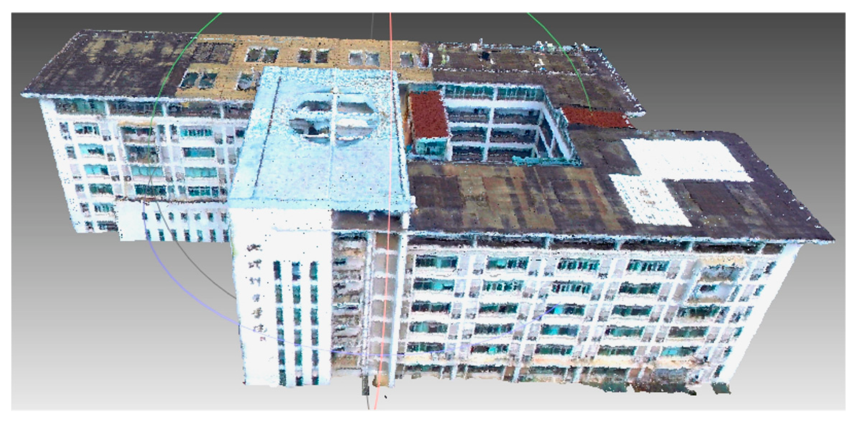
The oblique photogrammetry or airborne LiDAR is the main way to collect three-dimensional (3D) data of large-scale urban scenes [1,2]. However, the 3D model of an urban scene constructed via oblique photogrammetry or airborne LiDAR technology comprises a whole and a set of many objects [3]. Although this kind of reconstructed 3D model can satisfy the scene visualization requirements, it is difficult to perform recognition and attribute assignment to target objects. Further, it cannot be applied to spatial analysis. Thus, to obtain a meaningful 3D model of each building, the single building extraction processing should be performed on the buildings, which are the main objects in the 3D model [2]. However, in acquiring the building point cloud, due to the shielding of the building itself and other ground objects (such as vegetation), the collected building point cloud is incomplete and may contain some holes. Especially at the bottom of the building, the point cloud of facade surfaces is incomplete after filtering processing due to the shielding of vegetation and vehicles. For example, Figure 1 shows an example of a building point cloud; there are many holes at the bottom of the building due to the shielding of vegetation. Therefore, these holes need to be filled to obtain the complete point cloud for each single building, which can lay a foundation for the automatic construction of its 3D model.
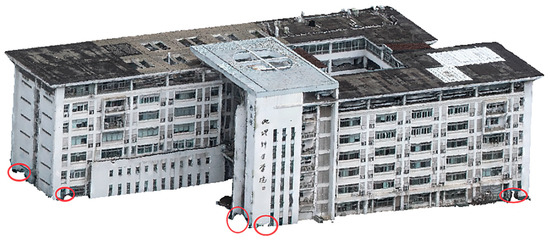
Figure 1.
Example of a building point cloud (red circles represent the location of holes).
The holes of the building point cloud can be classified into two groups. The first group consists of the holes in the building itself. For instance, while collecting the LiDAR data, some objects, such as windows, do not reflect the laser and appear as holes in the LiDAR data. The second type group consists of the holes generated by the shielding of objects, such as vegetation and vehicles; these holes are mainly located at the bottom of the building. The former type of hole is unique for the building and does not need to be repaired, whereas the latter is a blind area generated by the obstruction of obstacles in data acquisition. These holes do not belong to the structure of the building itself; they must be filled to achieve complete modeling of the building.
With the commonly used hole-filling methods, data fitting and interpolation are performed on the hole areas to complete the hole filling according to the similarity between each building hole and its neighborhood data. Such methods mainly include implicit surface fitting [4,5] and mesh model repairing [6], which can process holes of various shapes and sizes. However, they ignore the original data features of the building, and the repaired data are relatively smooth and do not retain the sharp features of the building completely.
To solve the problems of existing methods, a new hole-filling approach considering the local similarity among floors for a building point cloud is proposed. The proposed method can repair the holes of the building point cloud and lay a foundation for the complete modeling of a single building. More specifically, our contributions can be summarized as follows:
- (1)
- We propose a hole-filling method considering the local similarity among floors that can repair holes automatically without manual intervention in the processing.
- (2)
- Experimental results on three different buildings show that the proposed method outperforms the state-of-the-art hole-filling methods.
The remaining part of this paper is organized as follows: Section 2 briefly introduces related works. The principle of the proposed hole-filling method is introduced in Section 3. Section 4 presents the detailed experimental results and discussion. Finally, conclusions and future work are presented in Section 5.
2. Related Works
The existing hole-filling methods for point clouds are mainly based on surface fitting algorithms. Based on the high similarity between the hole and its neighborhood data, the existing methods perform interpolation repair on the hole by analyzing the data’s spatial correlations and using them to fit the surface model where the hole is located [7]. The commonly used surface fitting algorithms include the moving least squares (MLS) method [8], B-spline curve method [9,10,11], radial basis function interpolation (RBF) [5], and deep learning method [12].
Although the obvious features in the missing data area can be completely repaired by using the RBF to fit the hole surface, the constructed implicit surface is smooth, and it is difficult to ensure a smooth connection with the original data [13]. Wang proposed a hole-filling method in which the main idea is to first construct a mesh model for the point cloud, and then to repair the holes with an implicit surface [14]. However, this method was only suitable for small-sized holes. The feature point matching method uses the idea of “divide and conquer” to decompose the complex hole into several simple holes, and then uses the wave-front algorithm to complete the hole filling [15]. However, when the hole’s area is large and essential information is lost, the local repair effect of the hole is poor since the important feature points cannot be matched. Wang used the gray theory to complete the repair and refinement of the target surface, which only had an ideal performance for the specific model and lacked broad applicability to other models [16].
Brunton proposed another method to fill the holes of a point cloud [17]; it projected the hole’s boundary in the 3D models to the two-dimensional (2D) plane, used the improved Delaunay triangulation algorithm to divide the region of the hole on the 2D plane, and then used the minimized energy function to convert the 2D plane to the mesh surface in 3D space. Unfortunately, this method was limited by the size of the hole boundary and caused some damage to the original model to a certain extent. Based on Brunton’s method, Fortes proposed a shape feature determination method [4]. Based on the minimum energy function, it generated hole patches for the original holes. However, this method requires good quality data around the holes. Wang proposed a method based on feature line extraction to fill the holes [18]. Using this method, feature lines were first extracted to obtain the sequence of control points of each hole, and Non-Uniform Rational B-Splines (NURBS) was used to fit and fill the holes. Frias proposed a method of filling the holes based on the superposition and comparison of the two cutwaters [19]. First, two cutwaters are segmented, then the translation-fitting of the whole cutwater over the damaged one is performed. Second, the damaged cutwater can be reconstructed when two cutwaters of the bridge point cloud are correctly aligned. The method can obtain better results, but it requires much manual intervention in the processing; therefore, the method is difficult to apply to buildings in the city.
Although the methods mentioned above can complete the repair of the holes in a building point cloud, they ignore the building’s unique geometric and texture features in the filling process. The repair results for buildings with complex textures and geometric features are non-ideal, and the repaired data cannot be smoothly connected with the original data. These existing problems have motivated us to propose a new hole-filling method for a single building point cloud considering the inter-floor characteristics of the building. The proposed method can repair the holes and obtain the complete point cloud of the single building, which lays a foundation for constructing the 3D model of the single building.
3. Proposed Method
This section gives the main details of the proposed holes filling approach. First, the main idea of the proposed method is introduced. Then, the method of detecting holes in building facades is given. Next, the main processes of identifying building floors are presented. Finally, the hole-filling approach based on the local similarity among floors is proposed.
3.1. Main Idea
The geometric and textural features of high-rise buildings present some patterns, especially in China; features of the point cloud in similar parts between different floors of buildings have high similarity [20]. Our hole-filling method for a building point cloud is proposed. The main process is shown in Figure 2. First, the building point cloud is extracted from all point clouds, and the boundary of the hole is identified. Second, the building floors are identified according to the building’s height. Third, the similarities between the hole data and the same area of adjacent floors are calculated. Finally, the holes are filled, and a 3D model of the single building is obtained.
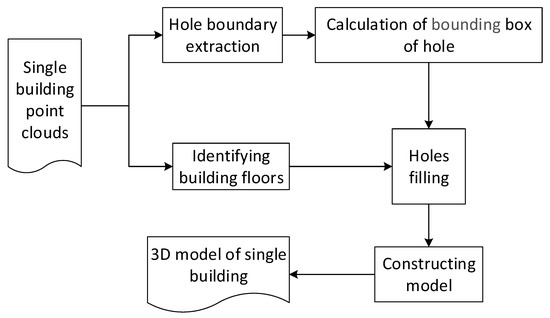
Figure 2.
Flow diagram of the proposed approach.
3.2. Building Rotation
Since the orientation of the building point cloud in the coordinate system is arbitrary, to better perform the following work and simplify the calculation, it is essential to rotate and translate the building parallel to the coordinate axis. The principal component analysis is a good approach to rotate buildings.
Given the building point cloud , its centroid is and the covariance matrix is COV. Then, the eigenvector of the covariance matrix is calculated, which represents three mutually perpendicular coordinate axes. Therefore, a rectangular spatial coordinate is established, which is the new coordinate system of the building point cloud. Finally, the rotation of the building point cloud is achieved. The of P can be obtained from Equation (1). The covariance matrix COV of P can be obtained from Equation (2).
The covariance matrix is computed; the three eigenvectors are ,, and respectively, and they correspond to the three mutually perpendicular directions of the building data. Then, the three eigenvectors are unitized and rotated parallel to the coordinate axis. When the point cloud is rotated, the z-axis of the building remains unchanged.
The rotation matrix R is computed using Equation (3), and all original data can be rotated to the new coordinate system. The relationship between the original point and new point in the new coordinate system is shown in Equation (4):
where is the translation value of coordinates. To simplify the calculation, the coordinates of the point cloud of the building are shifted near the origin. The coordinate of the point at the left bottom for the building is [0, 0, 0] when the building is shifted.
3.3. Hole Boundary Extraction
- (1)
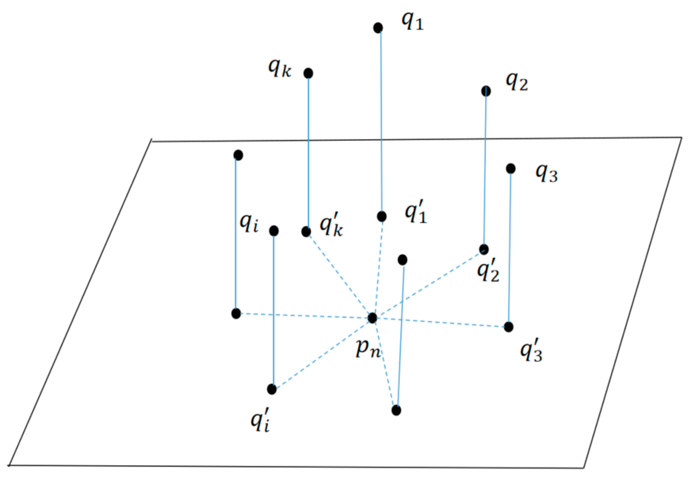
- Searching k nearest neighbor points and constructing the perpendicular plane of a normal vector
The k-d tree is a classical method of point cloud query which is a variant of a binary tree in multi-dimensional space [21]. Herein, the k-d tree was used to obtain the k nearest neighbor points (Q{}) of point pn. On how to choose the better k value, reference [22,23] gave some basic criteria. Based on reference [22,23], k is set as 20 in this paper. Afterward, points pn and Q are fitted into a spatial plane (x-y plane). Next, to compute the normal of as , the perpendicular plane of the normal vector (L) can be obtained from Equation (5):
Equation (5) is converted into the general form (Equation (6)), where D in Equation (6) can be converted into Equation (7):
To judge the uniformity of the distribution of k nearest neighbor points (Q), it is important to project Q on the perpendicular plane of the normal vector (L), which is shown in Figure 3.
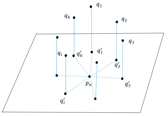
Figure 3.
k nearest neighbor points(Q) projected on the perpendicular plane of normal vector (L).
The coordinate of the neighboring point qi is (), and the coordinate of its projection point is . Thus, the projection point can be computed from Equation (8):
- (2)
- Identifying hole border points
The maximum angle difference is used to judge the uniformity of the distribution of k nearest neighbor points (Q) of point pn [24]. If the neighboring points are not distributed around the point pn, pn is viewed as the border point; otherwise, it is not. For instance, in Figure 4a, the neighboring points of the center point are not distributed around the center point; thus, it is a border point. In Figure 4b, the neighboring points of the center point are uniformly distributed around the center point; thus, it is not a border point.
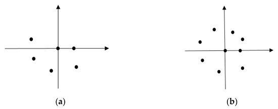
Figure 4.
Detection of the border point. (a) Border point, (b) no border points.
In Figure 3, the edge () is used as the starting edge, and the angles between each projection point and are computed. Then, these angles are sorted into ascending order: the maximum value () and minimum (0) values are added to the angle set; thus, a new ordered set () can be obtained. The differences in adjacent objects in are calculated from Equation (9), and the difference set can be obtained. If there exists an > threshold , the point is determined to be a border point. The selection of threshold is based on reference [22,23]; in reference [23], they give a range of threshold that does not exceed , and for a building point cloud, the threshold is . Therefore, the threshold is set as in this paper.
- (3)
- Connecting border points
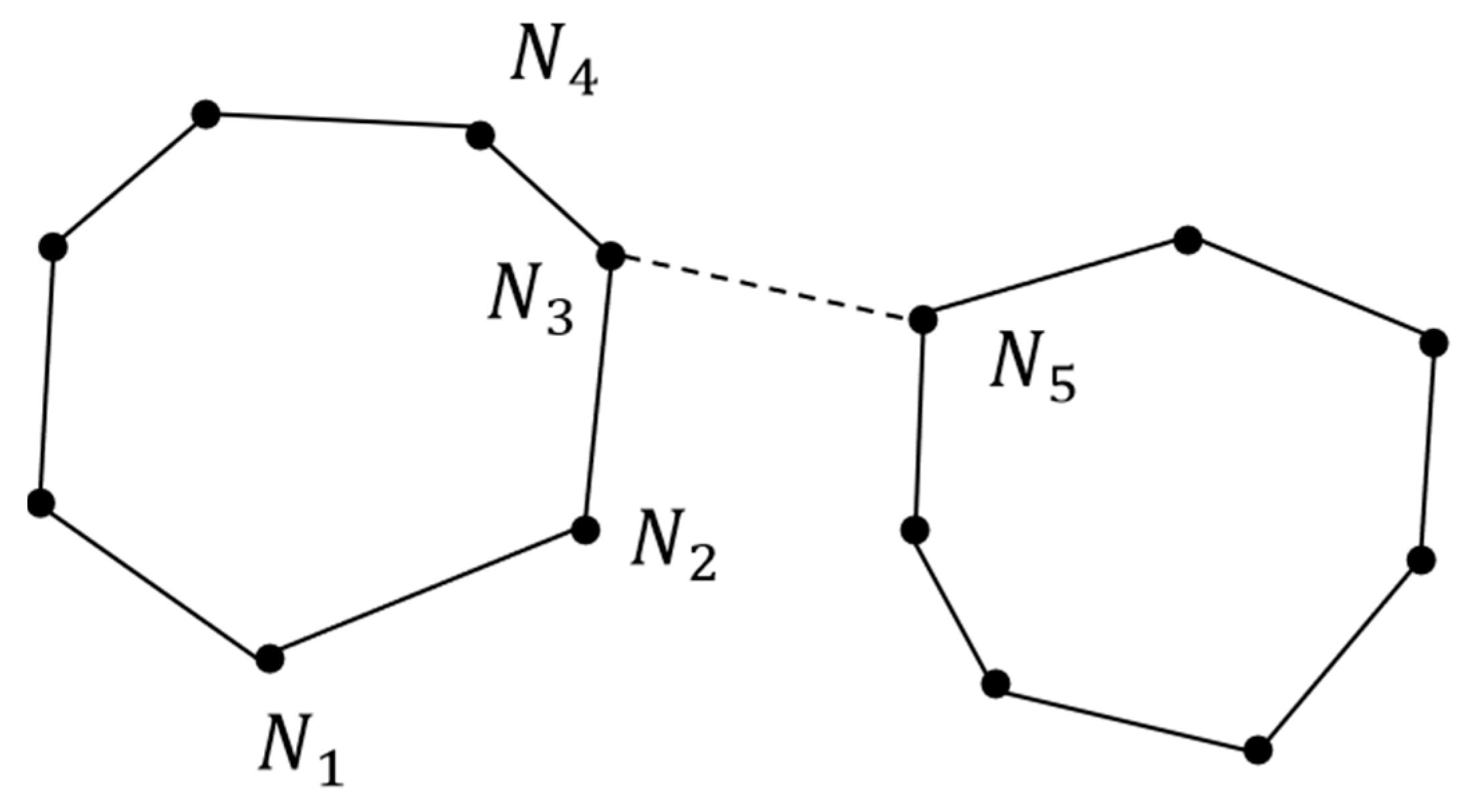
The border points are connected using the vector deflection angle (Equation (10)) and boundary coherence [22,23]. For example, the adjacent points of point are and (Figure 5). If only the distance is considered when the border points are connected, points , , and belong to the same boundary. However, they should belong to different boundaries. Thus, the vector deflection angle is used to sort the border points. The main processes of connecting border points are as follows: First, any border point can be viewed as the starting point, and then the boundary loop can be extracted using the breadth-first search. Next, any unconnected border point can be chosen as the initial point; the above process is performed. Finally, all boundaries can be identified exactly.
where Ni, Ni+1, and Ni+2 are adjacent points.

Figure 5.
Connection of border points.
3.4. Building Floor Identification
To fill holes by using similar features at the same place on different floors, it is essential to identify the different building floors. In identifying the building floors, the point cloud of the top appendage (such as the attic) and the basement are not considered. For instance, in Figure 1, there is a small attic that is located in the left front corner of the roof. The main processes of identifying the building floors are listed below:
Traversing all points, the maximum and minimum elevation () of the building point cloud can be found.
The 3D point clouds are projected on the spatial grid (the grid size (D) is two to three times the point cloud density [25]); this process is mainly to avoid the effect of false elevation.
The maximum elevation () of the point cloud in each grid unit is determined; the elevation value with the highest occurrence frequency is viewed as the evaluation of the roof elevation of the building ().
To ensure that the lowest elevation of the point cloud in each grid unit is the facade root of the building, the point with an elevation that is more than in the grid units is removed.
The lowest elevation () of the point cloud in each grid unit is determined, and the value with the highest occurrence frequency is viewed as the bottom elevation of the building ().
The actual number of floors of the building is N, which is set based on visual judgment; thus, the height of each floor is h (Equation (11)).
3.5. Filling Holes
Let the top height of each floor of the building with N floors be {}. Given the minimum bounding box of a hole , if and , the hole spans m () floors. The minimum bounding box of a similar area is . The coordinates of the data in a similar area and the hole are and , respectively.
The same area of the building’s adjacent floor is used to repair the holes of the building facade point cloud. According to Equation (12), the bounding box of the hole is shifted units upward, and the new bounding box of the hole can be obtained. If the new bounding box has complete data, the hole can be directly repaired. Otherwise, the bounding box of the hole continues to be shifted units upward. The holes can be wonderfully filled by the above processes; moreover, the filled results can contain the texture information as well as geometry information.
4. Experimental Evaluation and Discussion
Herein, Unmanned Aerial Vehicle (UAV) oblique photography was conducted by “DJI Phantom 4” on the Nanjing Normal University campus; the datasheet of the “DJI Phantom 4” is shown in Table 1. Moreover, Pix4D [26] was used for data processing of the oblique photography images to obtain the whole area point cloud. The building boundary was identified from the DOM, and the building point cloud was extracted. An experiment was performed based on the building point cloud, and the effectiveness and accuracy of the proposed method were evaluated. In the experiments, k was set as 20 and the threshold was set as .

Table 1.
DJI Phantom 4 main information.
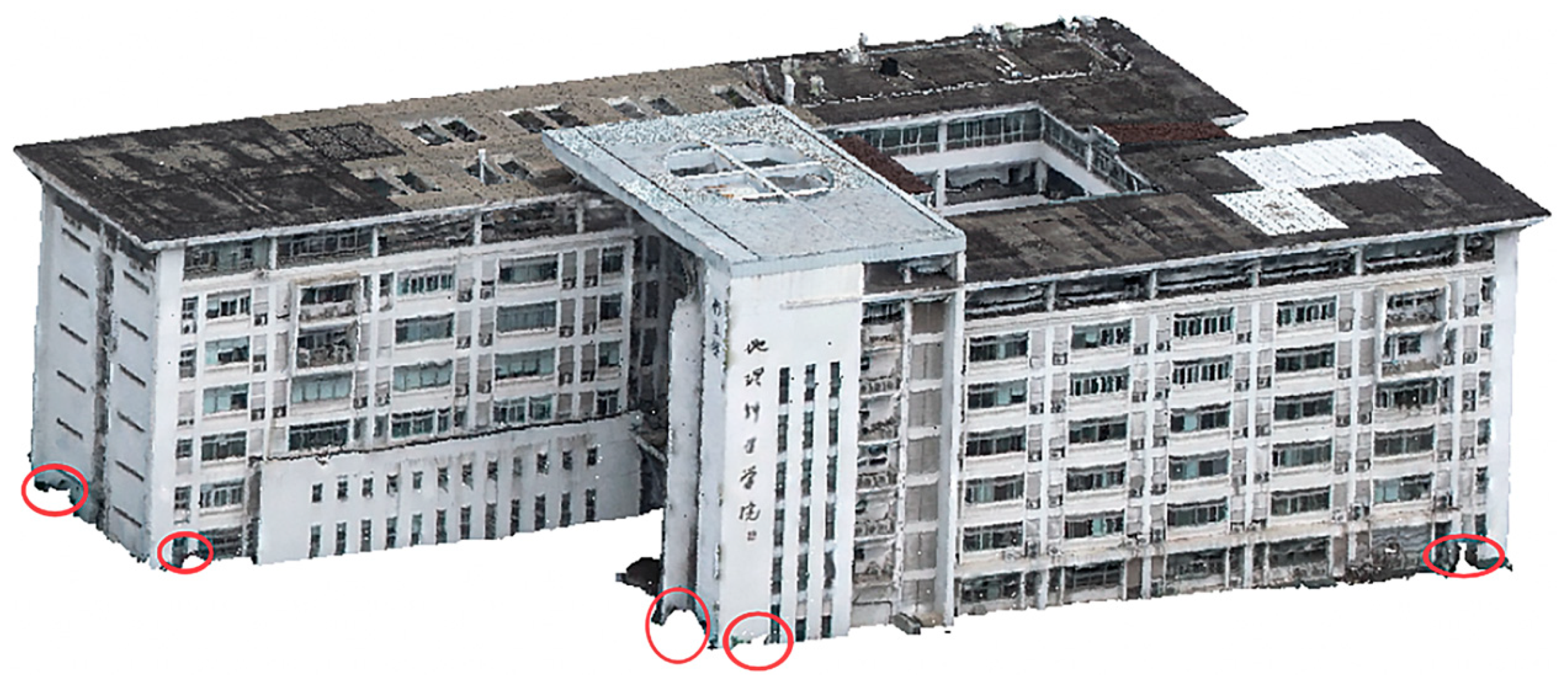
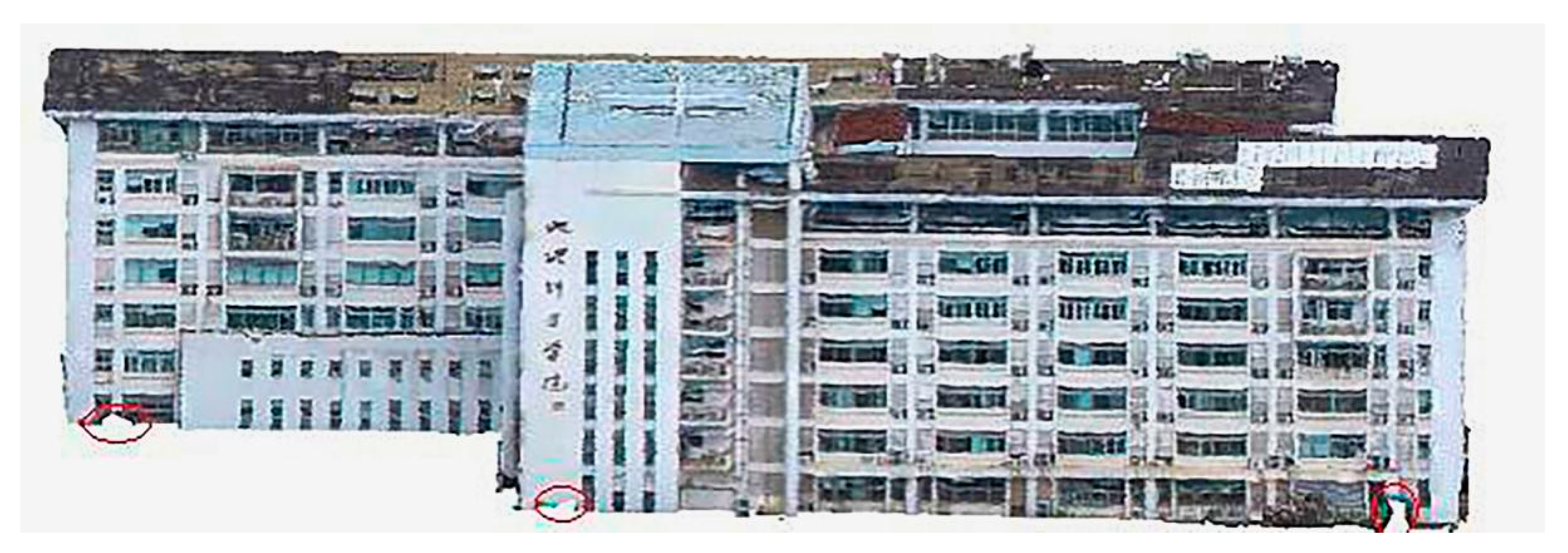
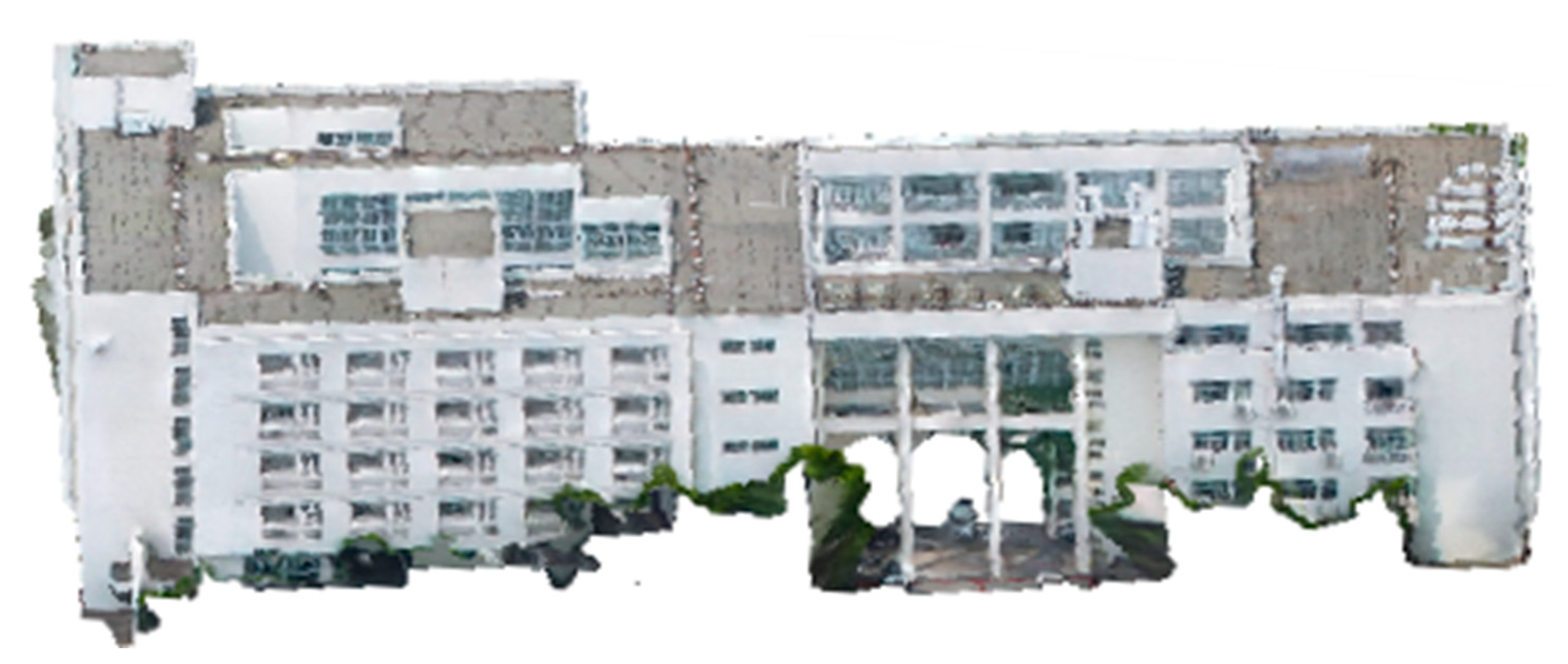
Figure 6 shows an extracted building point cloud, which is a pure point cloud that has filtered out vegetation and obstacles. Some holes that are marked by red circles appear on the facade surface of the building, which are mainly located on the bottom floor of the building near the ground.
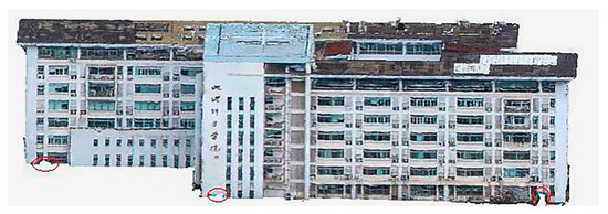
Figure 6.
Building point cloud with holes (red circles represent the location of holes).
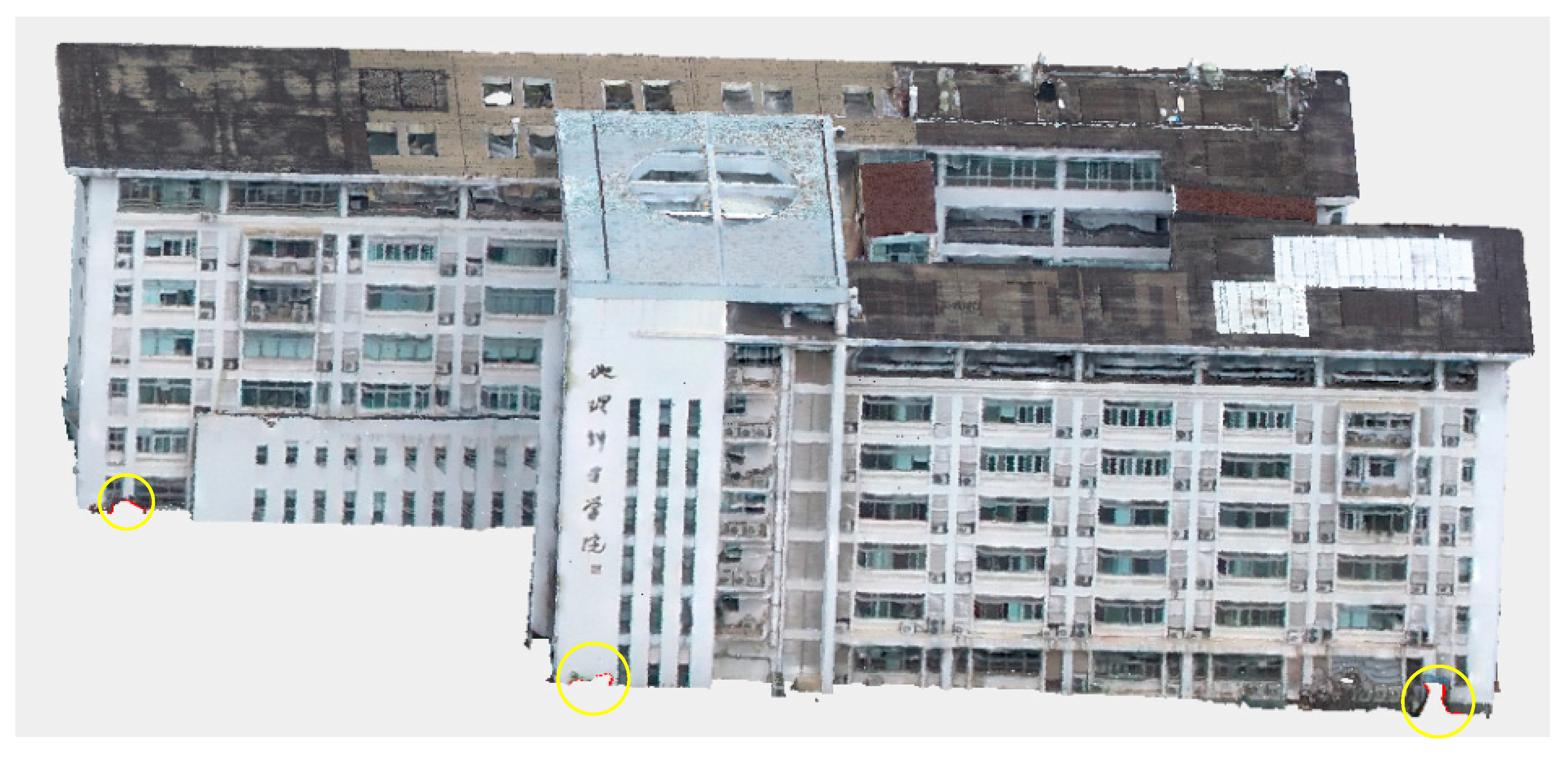
The important part of filling holes is to identify hole boundaries correctly. The 13 holes in the building were identified using the maximum angle difference. Figure 7 shows the holes in the front facade of the building; the red marks within the yellow circle are the identified hole boundaries. As depicted in Figure 7, the proposed method can identify the accurate boundary of all holes with different shapes and sizes. Since the holes are in different positions, they have complex features. Thus, it is a challenging task to fill the holes.
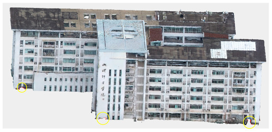
Figure 7.
Recognition results of hole boundaries (red points represent the identified border points; yellow circles represent the location of holes).
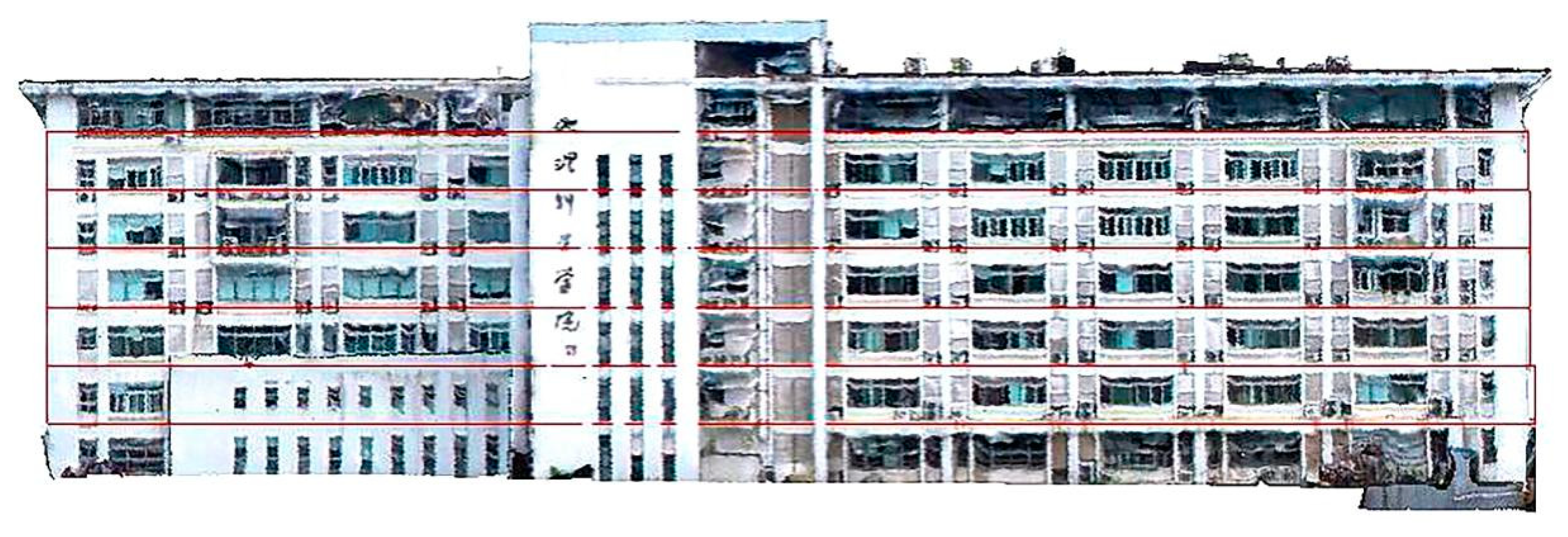
After the hole boundaries are obtained, the building floors are identified. The partitioned result is shown in Figure 8. The red lines indicate where each floor of the building is divided. The partitioned results are the same as the real floors of the building. Moreover, the building’s top appendage and bottom basement do not affect the partitioning result, which indicates the robustness and practicability of the proposed method.
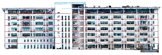
Figure 8.
Partitioned results of building floors (red horizontal lines represent building floors).
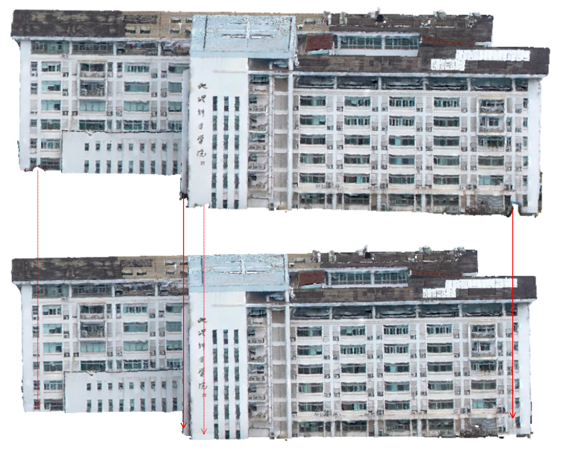
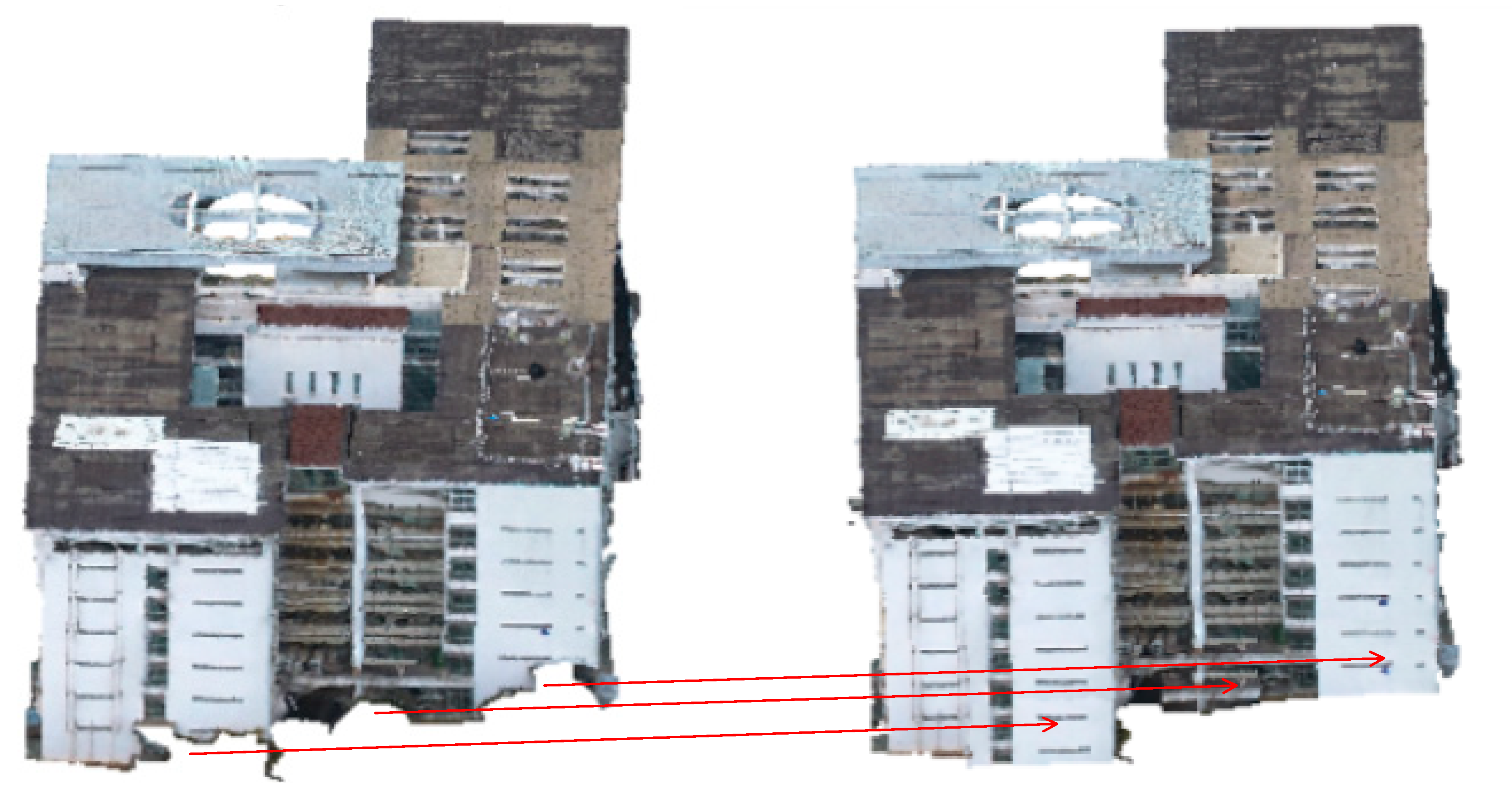
Some results of filling the holes are presented in Figure 9 and Figure 10, where the lower and right figures show the filled results of the front and lateral holes, respectively. The proposed method can wonderfully fill the holes and preserve their original features. Comparing the original data and filled results, it can be seen that the proposed method fills holes with different shapes and sizes quite well, and the complete building point cloud can be obtained. As expected, the filled results are the same as the original building.
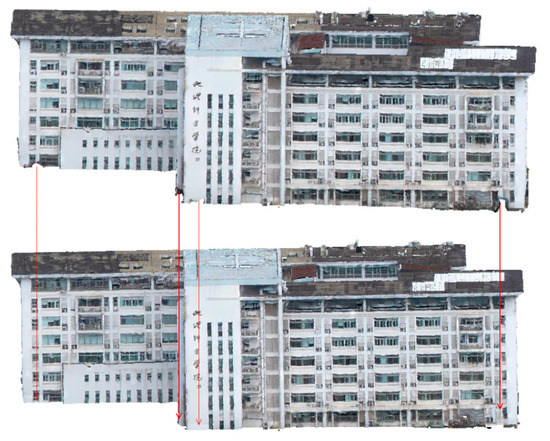
Figure 9.
Filled results of front holes (red lines represent the corresponding areas).
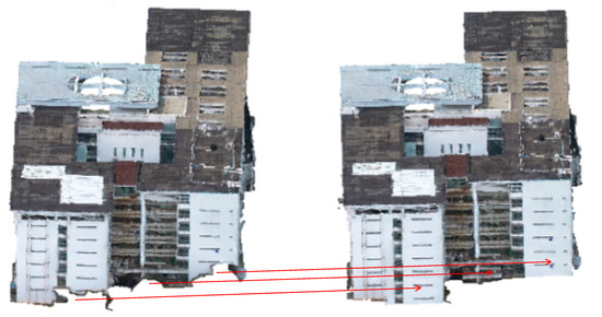
Figure 10.
Repaired results of lateral holes (red lines represent the corresponding areas).
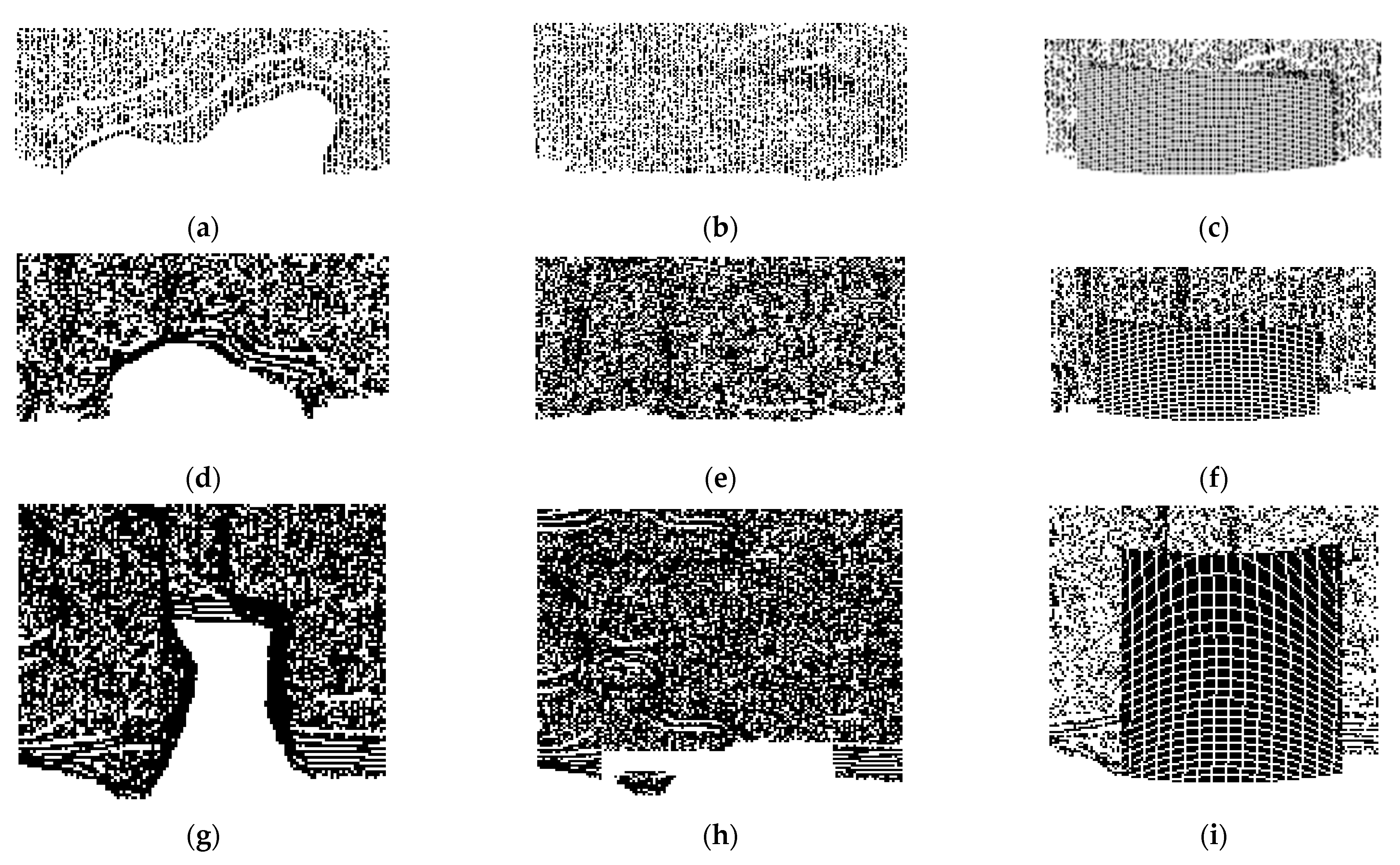
To better analyze the performance of the proposed method, it was compared with the MLS [8]. Figure 11 presents the filled results of some holes using the MLS and our method, respectively. Figure 11a,d,g shows the holes before filling; Figure 11b,e,h shows the repaired results using the proposed method. Figure 11c,f,i shows the filled results by the MLS. The point cloud of the repaired holes using the MLS is evenly distributed, but cannot be smoothly transitioned from the original point cloud, which is quite different from the original data. In contrast, the filled result by the proposed method can be smoothly connected with the original point cloud, which is similar to the distribution of the original building point cloud. Especially for the boundary, no discontinuity was found, and the filled result and the original point cloud can be connected well. Thus, the proposed method is superior to the MLS; the filled holes are more appropriate.
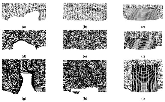
Figure 11.
Repaired results using moving least square and the proposed method. (a) Hole 1 before filling, (b) Filling hole 1 by our method, (c) Filling hole 1 by MLS, (d) Hole 2 before filling, (e) Filling hole 2 by our method, (f) Filling hole 2 by MLS, (g) Hole 3 before filling, (h) Filling hole 3 by our method, (i) Filling hole 2 by MLS.
To better evaluate and analyze the performance of the proposed method, some areas of buildings were artificially selected to dig holes with different features and sizes. Then, the artificial holes were filled using different methods, which are marked by red rectangles in Figure 12.

Figure 12.
The experimental area of artificial holes (red rectangles represent the location of artificial holes). (a) Artificial hole 1, (b) Artificial hole 2.
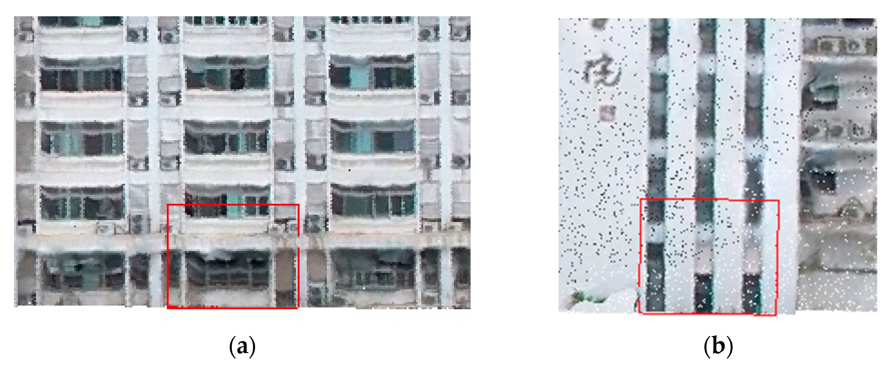
The filled results of artificial holes using different approaches are presented in Figure 13. Figure 13a,b shows the original point cloud of artificial holes 1 and 2, respectively; Figure 13c,d shows the corresponding repaired results using the proposed method; Figure 13e,f shows the corresponding filled results using the MLS. Overall, Figure 13 shows that the filled results using the proposed method are similar to the original building point cloud. Compared with Figure 13a,c, it is shown that the filled result can preserve the original building features and objects’ structural information, such as windows, quite well. Compared with Figure 13a,e, it is shown that the filled results using the MLS fit the smooth surface without preserving the details. Thus, the filled results cannot be smoothly connected with the original point cloud. Furthermore, although the artificial holes span two floors, the filled results using the proposed method are ideal.
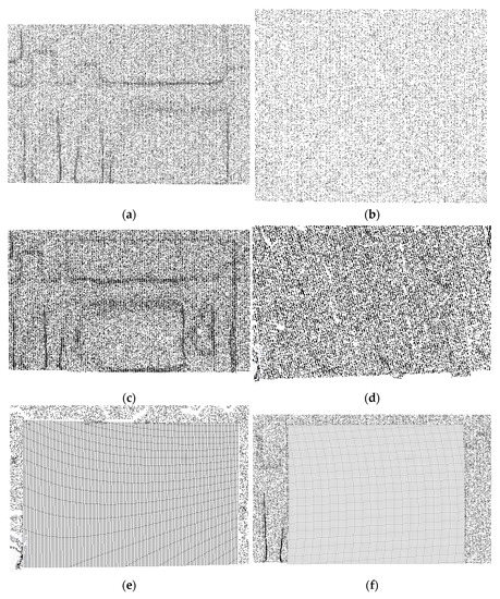
Figure 13.
Filled results of artificial holes using different methods. (a) Original point cloud of artificial holes 1, (b) Original point cloud of artificial hole 2, (c) Filling artificial hole 1 by our method, (d) Filling artificial hole 2 by our method, (e) Filling artificial hole 1 by MLS, (f) Filling artificial hole 2 by MLS.
The filled results were further evaluated and analyzed using root mean square error (RMSE) [8]. Table 2 presents the RMSE of different filled results. The original data were viewed as real values to calculate the RMSE of the two methods. The RMSE of the proposed method is less than that of the MLS. Therefore, the accuracy of the proposed method is higher, and the filled results using the proposed method are similar to the original data.
Table 2.
Comparison of RMSE values of the proposed method and moving least square method.
Hence, the proposed method can effectively fill the complex holes of the building point cloud and preserve the original features of the building quite well, and the filled results are similar to the original building point cloud. From this comparison, we can see that the proposed method always outperforms the MLS. The 3D model of the single building can be constructed when the complete building point clouds are obtained; the result is shown in Figure 14. The 3D model has a complete surface that does not show any obvious holes. Therefore, the effectiveness and practicability of the proposed method can be verified.

Figure 14.
Three-dimensional model of a building.
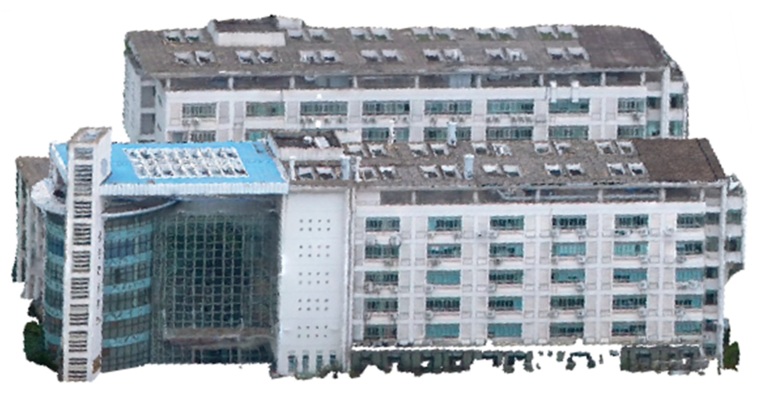
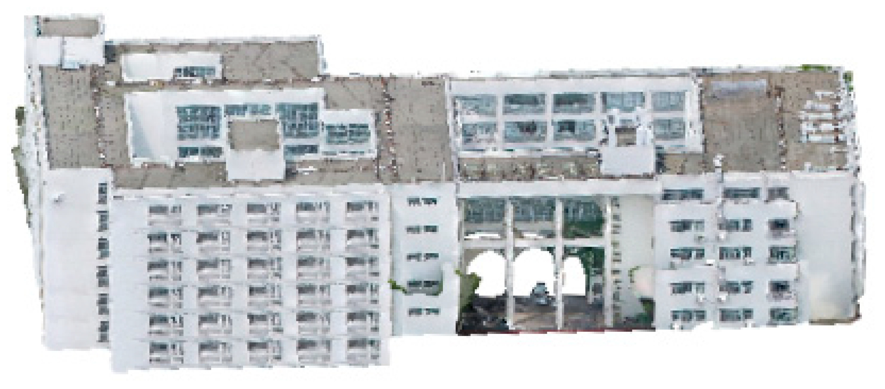
To better evaluate the effectiveness of the proposed method, the proposed hole-filling method is applied to two other buildings with different sizes of holes. Figure 15 and Figure 16 show building A and B before filling, respectively. Due to the shielding of vegetation and other ground objects, the collected building point cloud is incomplete and contains various holes, especially at the bottom of the two buildings. As shown in Figure 15, the facade point cloud of building A contains large holes, which are difficult to fill. From Figure 16, we can observe that the first-floor point cloud of building B contains very unique holes.
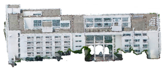
Figure 15.
Building A point cloud before filling.

Figure 16.
Building B point cloud before filling.
The proposed method is applied to building A; Figure 17 presents the filled result. We can observe that the different holes can be repaired and the original features and objects’ structural information can be preserved well. However, we can also find that the boundaries of large holes in two floors cannot be not filled well; some discontinuities are found. Figure 18 shows the repaired results of building B facade point cloud by the proposed method; it can be seen that the filled results preserve its original features. It can be seen that the proposed method can wonderfully fill the holes and preserve its original features. Moreover, the repaired result can be smoothly connected with the original point cloud, which is similar to the distribution of the original building point cloud.

Figure 17.
Filled results of building A by the proposed method.
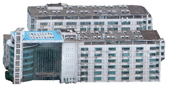
Figure 18.
Filled results of building B by the proposed method.
Comparative experimental results were examined to evaluate the proposed method using three different datasets. The results show that the filling method proposed in this paper successfully repairs the holes caused by the shielding of the building itself and other ground objects. The filled result by the proposed method can be smoothly connected with the original point cloud, which is similar to the distribution of the original building point cloud. Through comparison, we can see that the proposed method has greater reliability and outperforms the state-of-the-art holes filling method MLS. The proposed method presents an important advance in filling holes; it can repair holes automatically without manual intervention in the processing. Therefore, it has value in the field of 3D geospatial information collection based on photogrammetry.
Although the proposed method shows a major improvement in filling holes, several aspects can be improved. First, the filled results for the large holes in more than two floors show some discontinuities, especially on the boundary. Second, the proposed method could be improved to be applied to atypical buildings, especially opera houses or stadiums.
5. Conclusions
In the view of the application targets of constructing 3D models of buildings, the holes of the building facade point cloud need to be filled. This paper proposes a novel method for filling holes of the building facade point cloud considering local similarity among floors. More importantly, the proposed method can fill holes automatically without manual intervention in the processing. The experimental results demonstrate that the proposed method can fill the holes caused by the shielding of the building itself and other ground objects (such as vegetation) quite well, and completely preserve the building’s original geometric and textural features. Compared with the state-of-the-art method MLS, the proposed method can better preserve the original features of the building facades point cloud and has greater accuracy; moreover, the filled results can be smoothly connected with the original data. Thus, the filled result using the proposed method can better provide the complete building point cloud, and the 3D model of the building can be constructed based on these data. Although the proposed method represents a great advantage in filling holes, some limitations need to be addressed; for example, the proposed method is difficult to apply to floor buildings and atypical buildings.
In the next work, we intend to construct a refinement 3D model of the building, such as indoor. Second, for some buildings with atypical facades, mathematical morphology [27] could be a better method for filling large holes.
Author Contributions
X.M., Y.W. and Y.S. provided the core idea for this study. X.M. and Y.W. implemented the method and carried out the experimental evaluation. X.M., Y.W. and Y.S. wrote the main manuscript. Y.S., K.Z., J.Q. and Y.H. provided comments and suggestions for this paper. All authors have read and agreed to the published version of the manuscript.
Funding
This work is supported by the Key Fund of the National Natural Science Foundation of China (grant number 41631175), the Natural Science Foundation of Jiangsu Province (grant number BK20201372), and the Open Fund of Smart Health Big Data Analysis and Location Services Engineering Lab of Jiangsu Province (grant number SHEL221002).
Institutional Review Board Statement
Not Applicable.
Informed Consent Statement
Not Applicable.
Data Availability Statement
Not Applicable.
Conflicts of Interest
The authors declare no conflict of interest.
References
- Yalcin, G.; Selcuk, O. 3D city modelling with oblique photogrammetry method. Procedia Technol. 2015, 19, 424–431. [Google Scholar] [CrossRef] [Green Version]
- Lesparre, J.; Gorte, B. Simplified 3D city models from LIDAR. In Proceedings of the ISPRS—International Archives of the Photogram-metry Remote Sensing and Spatial Information Sciences, Melbourne, Australia, 25 August–1 September 2012; pp. 1–4. [Google Scholar]
- Tarsha Kurdi, F.; Awrangjeb, M.; Munir, N. Automatic filtering and 2D modelling of LiDAR building point cloud. Trans. GIS J. 2021, 25, 164–188. [Google Scholar] [CrossRef]
- Fortes, M.A.; Gonzalez, P.; Palomares, A.; Pasadas, M. Filling holes with shape preserving conditions. Math. Comput. Simul. 2015, 118, 198–212. [Google Scholar] [CrossRef]
- Branch, J.W.; Prieto, F.; Boulanger, P. Method of hole-filling on triangular meshes using local radial basis function. DYNA 2007, 74, 97–111. [Google Scholar]
- Xue, J.; Chen, Y.H. A Haptics-guided hole-filling system based on triangular mesh. Comput.-Aided Des. Appl. 2006, 3, 711–718. [Google Scholar]
- Chalmovianský, P.; Jüttler, B. Filling holes in point clouds. In Mathematics of Surfaces; Springer: Berlin/Heidelberg, Germany, 2003; pp. 196–212. [Google Scholar]
- Liang, P.; Zhou, G.Q.; Lu, Y.L.; Song, B. Hole-filling algorithm for airborne LIDAR point cloud. Int. Arch. Photogramm. Remote Sens. Spat. Inf. Sci. 2020, 42, 739–745. [Google Scholar] [CrossRef] [Green Version]
- Fortes, M.A.; González, P.; Pasadas, M.; Rodríguez, M.L. Hole filling on surfaces by discrete variational splines. Appl. Numer. Math. 2012, 62, 1050–1060. [Google Scholar] [CrossRef]
- Tekumalla, L.S.; Cohen, E. Reverse engineering point clouds to fit tensor product B-spline surfaces by blending local fits. arXiv 2014, arXiv:1411.5993. [Google Scholar]
- Yang, Z.; Deng, J.; Chen, F. Fitting unorganized point clouds with active implicit B-spline curves. Vis. Comput. 2005, 21, 831–839. [Google Scholar] [CrossRef]
- Tabib, R.A.; Jadhav, Y.V.; Tegginkeri, S.; Gani, K.; Desai, C.; Patil, U.; Mudenagudi, U. Learning-based hole detection in 3D point cloud towards hole filling. Procedia Comput. Sci. 2020, 171, 475–482. [Google Scholar] [CrossRef]
- Chen, C.; Cheng, K.; Liao, H.M. A sharpness dependent Approach to 3D polygon mesh hole filling. In Eurographics; Eurographics Digital Library: Geneve, Switzerland, 2005; pp. 13–16. [Google Scholar]
- Wang, J.; Oliveira, M. A hole-filling strategy for reconstruction of smooth surfaces in range images. In Proceedings of the Brazilian Symposium on Computer Graphics and Image Processing, Sao Carlos, Brazil, 12–15 October 2003; pp. 11–18. [Google Scholar]
- Wang, X.; Liu, X.; Lu, L.; Li, B.; Cao, J.; Yin, B.; Shi, X. Automatic hole-filling of CAD models with feature-preserving. Comput. Graph. 2012, 36, 101–110. [Google Scholar] [CrossRef]
- Wang, L.C.; Hung, Y.C. Hole filling of triangular mesh segments using systematic grey prediction. Comput. Aided Des. 2012, 44, 1182–1189. [Google Scholar] [CrossRef]
- Brunton, A.; Wuhrer, S.; Shu, C.; Bose, P.; Demaine, E.D. Filling holes in triangular meshes by curve unfolding. In Proceedings of the IEEE International Conference on Shape Modeling and Applications, Beijing, China, 26–28 June 2009; pp. 66–72. [Google Scholar]
- Wang, Y.; Tang, J.; Zhao, Y.; Hao, W.; Ning, X.; Lv, K. Point cloud hole filling based on feature lines extraction. In Proceedings of the 2017 International Conference on Virtual Reality and Visualization (ICVRV), Zhengzhou, China, 21–22 October 2017; pp. 61–66. [Google Scholar]
- Frias, J.B.; Sánchez-Rodríguez, A. Point Cloud Approach For Modelling The Lost Volume of The Fillaboa Bridge Cutwater. Surv. Geospat. Eng. J. 2021, 30, 13–20. [Google Scholar]
- Du, S.; Zhang, Y.; Zou, Z.; Xu, S.; He, X.; Chen, S. Automatic building extraction from LiDAR data fusion of point and grid-based features. ISPRS J. Photogramm. Remote Sens. 2017, 130, 294–307. [Google Scholar] [CrossRef]
- Bentley, J.L. Multidimensional binary search trees in database applications. IEEE Trans. Softw. Eng. 1979, SE-5, 333–340. [Google Scholar] [CrossRef]
- Bendels, G.H.; Schnabel, R.; Klein, R. Detecting Holes in Point Set Surfaces. J. WSCG 2006, 14, 89–96. [Google Scholar]
- Truong, H.L.; Laefer, D.F.; Hinks, T.; Carr, H. Combining an angle criterion with voxelization and the flying voxel method in reconstructing building models from LiDAR data. Comput.-Aided Civ. Infrastruct. Eng. 2013, 28, 112–129. [Google Scholar] [CrossRef] [Green Version]
- Kai, C.; Kai, Z.; Da, Z.; Chi, Z. The boundary extraction and hole restoration method of point cloud of 3D laser scanner for mine. In Proceedings of the 2020 IEEE 3rd International Conference on Information Systems and Computer Aided Education (ICISCAE), Dalian, China, 27–29 September 2020. [Google Scholar]
- Hanning, R.P. Spatial Data Analysis: Theory and Practice; Cambridge University Press: Cambridge, UK, 2003. [Google Scholar]
- Pix4D. Pix4D Mapper User Manual; Pix4D: Prilly, Switzerland, 2013. [Google Scholar]
- Balado, J.; Van Oosterom, P.; Díaz-Vilario, L.; Meijers, M. Mathematical morphology directly applied to point cloud data. ISPRS J. Photogramm. Remote Sens. 2020, 168, 208–220. [Google Scholar] [CrossRef]


Publisher’s Note: MDPI stays neutral with regard to jurisdictional claims in published maps and institutional affiliations. |
© 2022 by the authors. Licensee MDPI, Basel, Switzerland. This article is an open access article distributed under the terms and conditions of the Creative Commons Attribution (CC BY) license (https://creativecommons.org/licenses/by/4.0/).