Article

Heterogeneous Urban Thermal Contribution of Functional Construction Land Zones: A Case Study in Shenzhen, China

1
Key Laboratory for Urban Habitat Environmental Science and Technology, School of Urban Planning and Design, Peking University, Shenzhen 518055, China
2
Key Laboratory for Earth Surface Processes, Ministry of Education, College of Urban and Environmental Sciences, Peking University, Beijing 100871, China
3
School of Resource and Environmental Sciences, Wuhan University, Wuhan 430079, China
*
Author to whom correspondence should be addressed.
Remote Sens. 2022, 14(8), 1851; https://doi.org/10.3390/rs14081851
Submission received: 27 February 2022 / Revised: 8 April 2022 / Accepted: 9 April 2022 / Published: 12 April 2022
(This article belongs to the Special Issue Geographical Analysis and Modeling of Urban Heat Island Formation)

Abstract

:
Anthropogenic interferences through various intensive social-economic activities within construction land have induced and strengthened the Urban Heat Island (UHI) effects in global cities. Focused on the relative heat effect produced by different social-economic functions, this study established a general framework for functional construction land zones (FCLZs) mapping and investigated their heterogeneous contribution to the urban thermal environment, and then the thermal responses in FCLZs with 12 environmental indicators were analyzed. Taking Shenzhen as an example city, the results show that the total contribution and thermal effects within FCLZs are significantly different. Specifically, the FCLZs contribution to UHI regions highly exceeds the corresponding proportions of their area. The median warming capacity order of FCLZs is: Manufacture function (3.99 °C) > Warehousing and logistics function (3.69 °C) > Street and transportation function (3.61 °C) > Business services function (3.06 °C) > Administration and public services function (2.54 °C) > Green spaces and squares function (2.40 °C) > Residential function (2.21 °C). Both difference and consistency coexist in the responses of differential surface temperature (DST) to environmental indicators in FCLZs. The thermal responses of DST to biophysical and building indicators in groups of FCLZs are approximately consistent linear relationships with different intercepts, while the saturation effects shown in location and social-economic indicators indicate that distance and social-economic development control UHI effects in a non-linear way. This study could extend the understanding of urban thermal warming mechanisms and help to scientifically adjust environmental indicators in urban planning.

Graphical Abstract

1. Introduction

Intensive social-economic activities in urban areas have produced severe and irreversible interferences on natural landscape patterns and climate conditions in the urbanization processes [1,2,3]. According to [4], more than two-thirds of the world population will live in cities and modern towns by 2050. Over the decades, Urban Heat Islands (UHI) has already received critical attention [5,6]. Due to the induced heat threats and health risks to urban residents [7,8], UHI has become one of the key issues in the realization of sustainable urban development goals (SDG11) [9,10].
As a proxy in the social-ecological process of human activities on the natural environment, land use and land cover change (LUCC) have been considered the main drivers of UHI effects. The existing literature on UHI has revealed that urban land use and the resulting changes in surface biophysical properties of the landscape have led to the energy unbalance of the thermal environment [11,12,13], and the thermal difference between urban and rural areas in local regions have been the main object in UHI studies. To date, various studies have investigated the relationship between UHI and urban climate-related properties from different perspectives from urban land cover and land use differences. For example, the local climate zones (LCZ) framework [14] provides a basic framework to map land surface into 17 types of urban climate zones according to urban physical structure parameters [15,16,17] and evaluate UHI effects [18,19,20]. Urban Function Zones (UFZ) [21] is another LUCC scheme in UHI studies that divides the whole urban area into sub-zones in consideration of similar social-economic activities in the local blocks. General findings that the causes and characteristics of UHI are closely related to the landscape patterns and environmental parameters of the land surface have been demonstrated in many academic publications [22]. It has been argued that the spatial heterogeneity of land surface temperature (LST) across LCZ or UFZ is influenced by scale [5], composition [23], and patterns [24,25] in categories of the surface landscape. Conclusions about differentiated thermal effects between impervious surfaces [26] and green-blue landscapes [27] have been applied to provide empirical planning strategies to alleviate UHI effects.
However, there are still limitations in UHI planning practice and research. Landscape with natural cooling effects such as the waterbody [28], vegetation [29], and artificial green infrastructures (GI) [13,27,30,31] could help to alleviate urban heat island effects with natural-based solutions, while the fixed location and scale of areas of forests, rivers, and lakes mean that these methods are only locally effective and show a lack of extensibility in the whole area. The effects and causes of UHI have already been investigated at the block level in recent studies, however, blocks divided by road networks are frequently used as the basic research units in LCZ and UFZ frameworks, researchers may lose the delicate insight into the construction land of different functions in a single block caused by different sizes of the blocks in the real world. In addition, the quantitative distinction between anthropogenic and environmental heat in UHI studies remains unclear. The difference between anthropogenic and natural heat still needs further study. Therefore, it is crucial to measure the thermal contribution in urban construction land.
Understanding human activities in urban land and the resulting quantitative thermal effects would help to regulate human behaviors to control artificial heating effects on the urban environment. Nowadays, crowdsourced data like points of interest (POIs) are gradually used to promote urban mapping due to its directivity to specific social and economic activities and the lower cost and more convenient access than field surveys [32,33]. Compared to the visual features in remote sensing images [17,34,35,36], categories or tags of POIs, which are collected in the searching requirements of daily life and travel activities, could better quantify the patterns of human activities in the region [37,38] and provide a good option for anthropogenic heat measurement. However, they are established in different classification systems by commercial firms, e.g., AMap [39], Baidu Map [40], and Google Maps [41]. They are also usually inconsistent with the land use standards in the urban planning field. Moreover, the absolute difference in quantity across different categories of POIs and different research objectives make it a problem to determine the function in the research unit just by the quantities or densities [42]. Thus, we still need to integrate the advantages of POIs for the mapping of social-economic functions of construction land for urban planning and management in a more spatial-continuous way. When relocating and resizing the natural cooling area is diseconomy and impossible for the whole city [43], reasonable allocation of the function of construction land, after understanding its diversified thermal capacity and contribution to the urban thermal environment, may provide new scientific pathways for heat island effect reduction.
After more than 40 years of rapid development under the Reform and Opening policy, the urbanization rate of Shenzhen has continued to take the lead in China in the recent decade [44]. Thus, Shenzhen has become a megacity with high risks of the UHI effects [45] and limited natural cooling areas [46,47]. Taking Shenzhen as an example city, three questions are focused on: (1) Are there differential thermal effects within urban construction land among various social-economic functions? (2) What are the contributions of construction land with different social-economic functions to the UHI effect? (3) What are the response processes of thermal effects to the environmental factors in construction land? In this study, we proposed an extensible framework to map urban construction land for social-economic functions at the grid level into functional construction land zones (FCLZs) using POIs and then evaluated the relative thermal effects based on differential surface temperature (DST) among urban areas to the surrounding areas. This study aims to provide implications for the regulation of the anthropogenic influences in UHI reduction in both the natural and social solutions for urban social-ecological problems.

2. Materials and Methods

2.1. Study Area

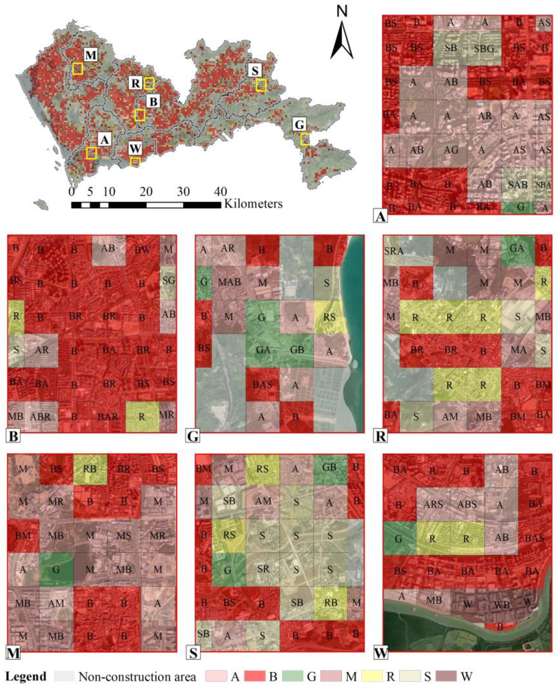
Shenzhen is a hilly megacity (21°25′N~24°30′N, 111°12′E~115°35′E) with a population of 17.56 million. Situated on the south coastline of China’s mainland and adjutant to the Peral River in the west, Shenzhen has a subtropical monsoon climate with a rainy and hot summer for 8 months and dry winter of less than 1 month during average recent years. The highly utilized construction land with a wide range of functional types is now widely distributed around woody hills and water bodies in the city (Figure 1), even if under the control of the urban master plan. Therefore, Shenzhen is one of the first cities to face not only insufficient space for urban development but also many severe urban ecological problems, e.g., an urban heat island.

2.2. Data Sources

In this study, we used points of interest (POIs) data collected from AMap [48] in June 2019 to recognize FCLZ types. The Landsat 8 Collection 2 Level 2 Science Product (L2SP) data processed based on Landsat 8 OLI/TIRS images (Table 1) were downloaded from the USGS website [49] due to similar higher air temperature and less cloud cover (<5%). To obtain the natural land surface temperature in non-construction areas, we extracted the waterbody and woodland cover from GlobeLand30 (2020) dataset [50]. Building survey data with shape and floor were provided by the Planning and Natural Resources Bureau of Shenzhen [51]. DEM data from ASTER GDEMV2 [52], night light data from Visible Infrared Imaging Radiometer [53], and population data from Landscan [54] were also employed to take into account the influences of building, topography, urban economic development, and demographic factors to the urban thermal environment, respectively.

2.3. Methods

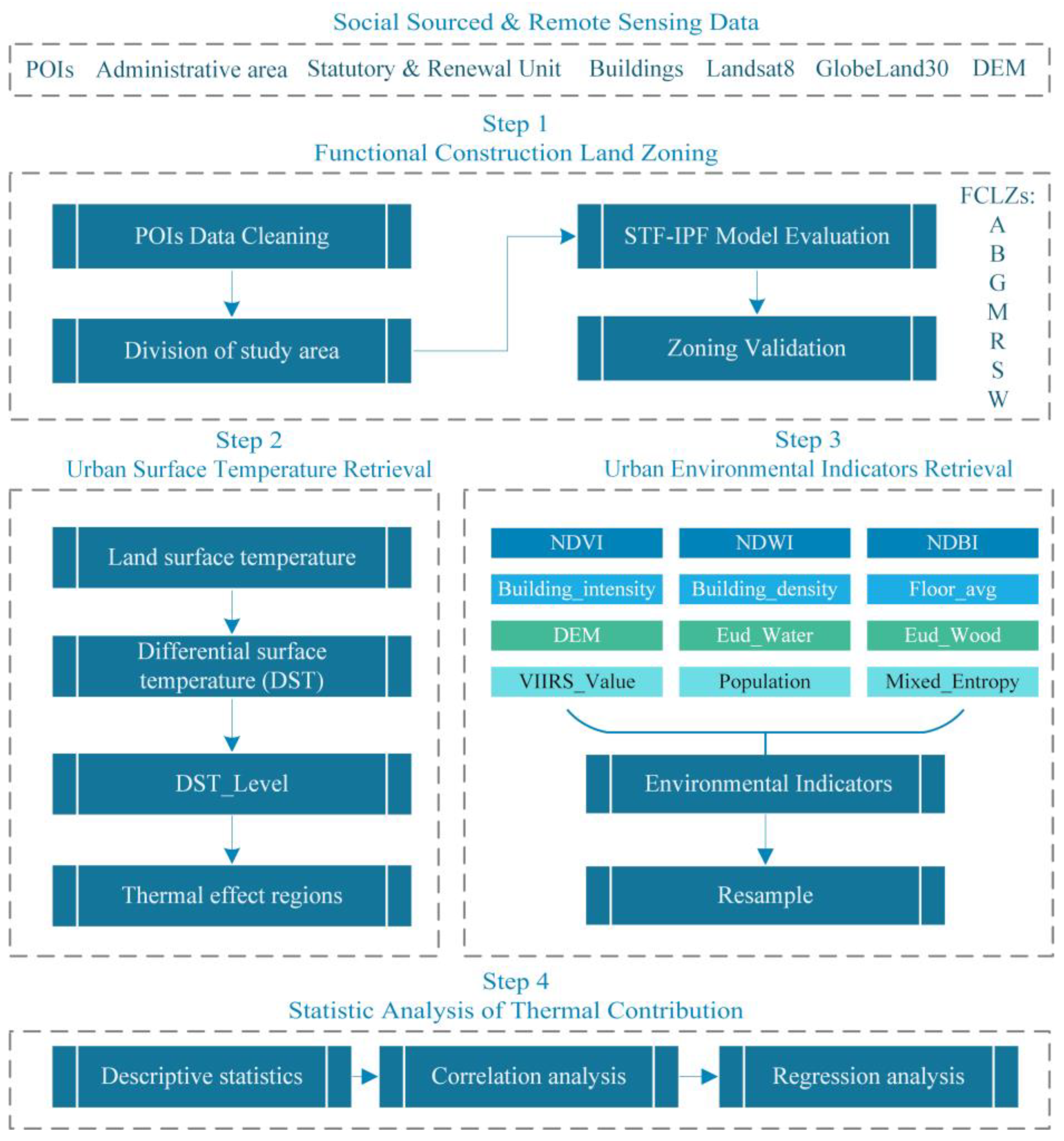
As shown in Figure 2, based on social sourced and remote sensing data, the research framework of this study consisted of three main steps.
First, functional construction land zoning (FCLZ) was implemented through the process of data cleaning, division of study area, spatial term frequency-inversed patches frequency (STF-IPF) model evaluation, and a results validation. Then, urban surface indicators including land surface temperature and four groups of environmental parameters, i.e., biophysical indicators, building indicators, location, and social-economic indicators, were retrieved and reprocessed across FCLZS using domain-based approaches. Finally, statistical analysis methods were used to explore the relationship between DST and environmental parameters in FCLZs. Next, those key processes are described in detail.

2.3.1. Functional Construction Land Zoning

  • Division of study area
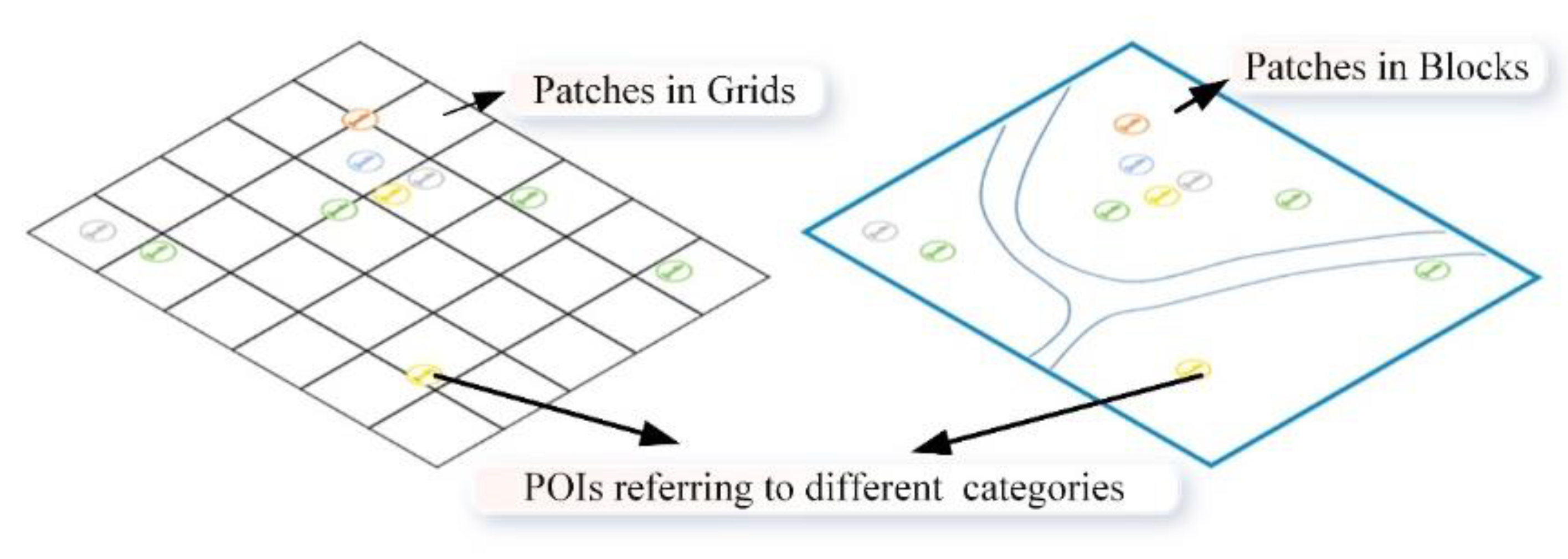
To depict the actual functional construction land in a more precise way, the first step was to divide the whole urban space into continuous grids at a certain scale to break the traditional boundary divided by road networks (Figure 3). An appropriate grid scale should be able to make the recognition results of functional constructional land as close as possible to reflect the spatial distribution and the focused problems. It was considered that 500 m might be enough distance to capture neighboring POIs in cities [55,56]. Therefore, we divided Shenzhen into 8575 grids at a scale of 500 m.
2.
Matching POIs attributions to functional construction land zones
To facilitate the FCLZs to guide urban planning and construction land use, we reclassified the POIs collected from AMap according to [57] into 7 types of construction land use by their defined categories and tags (Table A1), i.e., Residential function (R), Administration and public services function (A), Business services function (B), Green spaces and squares function (G), Street and transportation function (S), Manufacture function (M), and Warehousing and logistics function (W).
3.
Calculation of POIs representativeness in patches
Different types of POIs usually correspond to various degrees of public awareness although they have differences in quantity. For instance, the commercial service facilities such as stores, supermarkets, catering, and so on, are always around some places in large numbers while the more concerned POIs in urban planning, e.g., railway stations, logistics parks, or large-scale residential communities may have only one or several POIs. As a consequence, density and frequency methods [42,58] (Equation (1)) often mistakenly identify the functional construction land zone type based on biased quantity observation caused by differences in the number of collected points.
P O I _ D e n s i t y i , j = C o u n t   o f   P O I   m a t c h e d   t o   f u n c t i o n   j   i n   P a t c h   i T o t a l   C o u n t   o f   P O I   i n   P a t c h   i
Inspired by the Term Frequency-Inversed Document Frequency (TF-IDF) model (Equation (2)) [59] in the field of Natural Language Process (NLP), we proposed a Spatial Term Frequency-Inversed Patches Frequency (STF-IPF) model in consideration of both the amount and the global significance to recognize representative functional construction land types (Equation (3)).
T F _ I D F = C o u n t   o f   w o r d   o c c u r a n c e s T o t a l   w o r d s   i n   d o c u m e n t × l o g T o t a l   n u m b e r   o f   d o c s N u m b e r   o f   d o c s   w o r d   i s   i n
S T F _ I P F = C o u n t   o f   P O I   m a t c h e d   t o   s p e c i f i c   f u n c t i o n   T o t a l   n u m b e r   o f   P O I   i n   p a t c h e s × l o g T o t a l   n u m b e r   o f   p a t c h e s N u m b e r   o f   p a t c h e s   w h e r e   s p e c i f i c   P O I   a r e   i n
Given a study area divided into patches with a total number of m and a set of POIs matched to m kinds of functional construction land, then the vector UNump j and the matrix N U could be defined as the following Equations (4) and (5), where N u i , j is the number of POIs in the patch i matched functional construction land type j .
UNump j = ( N u 1 , j , N u 2 , j , , N u m 1 , j , N u m , j )
N U = ( UNump 1 T , UNump 1 T , , UNump n 1 T , UNump n T )
Then the normalized STF-IPF value for function j in patch i could be calculated according to Equation (6), which takes both numbers and repetitiveness into account by combining Equations (1) and (3).
S T F _ I P F i , j = N u i , j N u i , j j = 1 n N u i , j log m C O U N T ( UNump j , N u m , j > 0 ) i = 1 m N u s i , j N u i , j j = 1 n N u i , j log m C O U N T ( UNump j , N u m , j > 0 )
where C O U N T ( UNump j , N u m , j > 0 ) calculates the counts of patches where the functional construction land zone type j is not null. Higher normalized S T F _ I P F i , j means that functional construction land zone type j in patch i is more dominant and distinct from other types.
4.
Recognition vectors evaluation
As shown in Equation (7), an FCLZ recognition vector for patch i could be constructed after sorting the value of normalized STF_IPF values in the descending order with the corresponding functional zone type index j .
R e c _ v e c i = ( S T F _ I P F m a x i , j , S T F _ I P F s e c o n d a r y i , j , , S T F _ I P F m i n i , j )
The corresponding functions in the vector whose cumulative percentage is greater than a threshold value ε (0~100%) are defined as the functions of the patches, and the function with the maximal value is the main function in the patch. If there is no POI in the patch, the type is set to a non-construction area (N). According to suggestions on compatible types and proportions of urban construction land [57], ε was set to 70%. Therefore, we could infer the FCLZs types in each patch by evaluating the recognition vectors, and then describe the mixed status of FCLZs by calculating the mixed entropy in each patch by Equation (8).
M i x e d _ e n t r o p y = j = 1 n ( S T F _ I P F j ln S T F _ I P F j )
In this study, we implemented the above processes in python scripts.

2.3.2. Urban Surface Temperature Retrieval

The land surface temperature (LST) data were derived from Landsat 8 Collection 2 Level 2 Science Product (L2SP) [49]. This product provides thermal infrared bands using the Radiative Transfer Equation method [60] after radiometric calibration and atmospheric correction. Digital numbers (DN) were converted to land surface temperature ( L S T ) using Equation (9).
L S T = D N × S F + A F 273.15
where D N is the digital number for a given pixel. S F and A F are the multiplicative and additive scale factors of ST products, and their values are 0.00341802 and 149, respectively. The item 273.15 is the additive factor that converts L S T value from Kelvin to Celsius.
As there is no rural area in this concept but many forests in Shenzhen, we used the average L S T in the woodland ( L S T ¯ w o o d ) to reflect the natural surface land temperature because of the low impact of human activities. Then D S T could be calculated using Equation (10), which is a more reprehensive and comparable indicator to quantify the urban thermal environment change induced by human activities.
D S T = L S T L S T ¯ w o o d

2.3.3. Urban Environmental Indicators Retrieval

5.
Biophysical indicators
L2SP also provides surface reflectance (SR) data in 9 bands processed by the LaSRC algorithm after calibration and atmospheric correction routines [61]. Similar to Equation (9), the SR data was converted from DN value to reflectance using Equation (11).
S R i = D N × S F + A F
where S R i is the digital number for a given pixel in band i . S F = 0.0000275 , A F = 0.2 . The valid value range for each band except band 6 (1~65,535) is from 7272 to 43,636.
Then based on the previous findings, the normalized difference vegetation index (NDVI), normalized difference water index (NDWI), and normalized building index (NDBI) were calculated as indicators to quantify the surface bio-physical characters considering vegetation cover [26,62], moisture content [28,63], and building materials [64,65] in the land surface.
6.
Building indicators
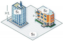
Buildings are still the most important feature in the construction area [25,66,67], thus we designed four building indicators (Table 2) using building survey data to quantify the building characters in the land grid.
7.
Location and social-economic indicators
DEM, Euclidean distance from the waterbody ( E u d _ W a t e r ) and wood ( E u d _ W o o d ) were used as location and neighborhood factors that would influence the urban thermal environment [19,68,69]. Night light data ( V I I R S _ V a l u e ) and Landscan data ( P o p u l a t i o n ) were indirect but explicit indicators to reflect the intensity of the economic development density and social activities intensity [70,71].
They were all extracted or calculated, resampled, and matched to the grids under the ArcGIS 10.2 platform.

2.3.4. Statistical Analysis

The Shapiro-Wilk normality test [72] was used to explore the distributions of DST among FCLZs, and the Kruskal-Wallis H test [73] was applied to find if there was a significant thermal difference between FCLZs. The Dunn test with Holm-Bofferoni correction [74] was used as a post hoc method in multiple comparisons to verify the specific difference in each pair of FCLZs. Then Spearman coefficients [75] between DST and environmental indicators among various types of FCLZs were calculated to figure out factors influencing the difference in thermal contribution capacity. Finally, multiple simple regression analyses were conducted to quantify the response processes of DST on environmental indicators.

3. Results

3.1. Mapping of FCLZs

According to the main functional type in each grid, grids with functional construction land of the 7 types are unevenly distributed in the 10 districts in Shenzhen (Figure 4).
To be more specific, the function of the most widely distributed grids which are agglomerated and distributed in clusters and strips is the Business services function (B), accounting for 41.62% of the total area of construction land. Grids of Administration and public services function (A), Street and transportation function (S), and Manufacture function (M) are clustered in patches of different sizes and show the aggregated distribution in each district, which takes up 19.77%, 14.90%, and 11.98% in the construction area, respectively. Residential function (R) and Green spaces and squares function (G) grids hold lesser area proportions of 6.94% and 4.16%, while they both show scattered distribution across districts. Warehousing and logistics function (W) grids with an area proportion of only 0.64% are significantly lower than others, which are distributed mainly at the edge and the center of every district.
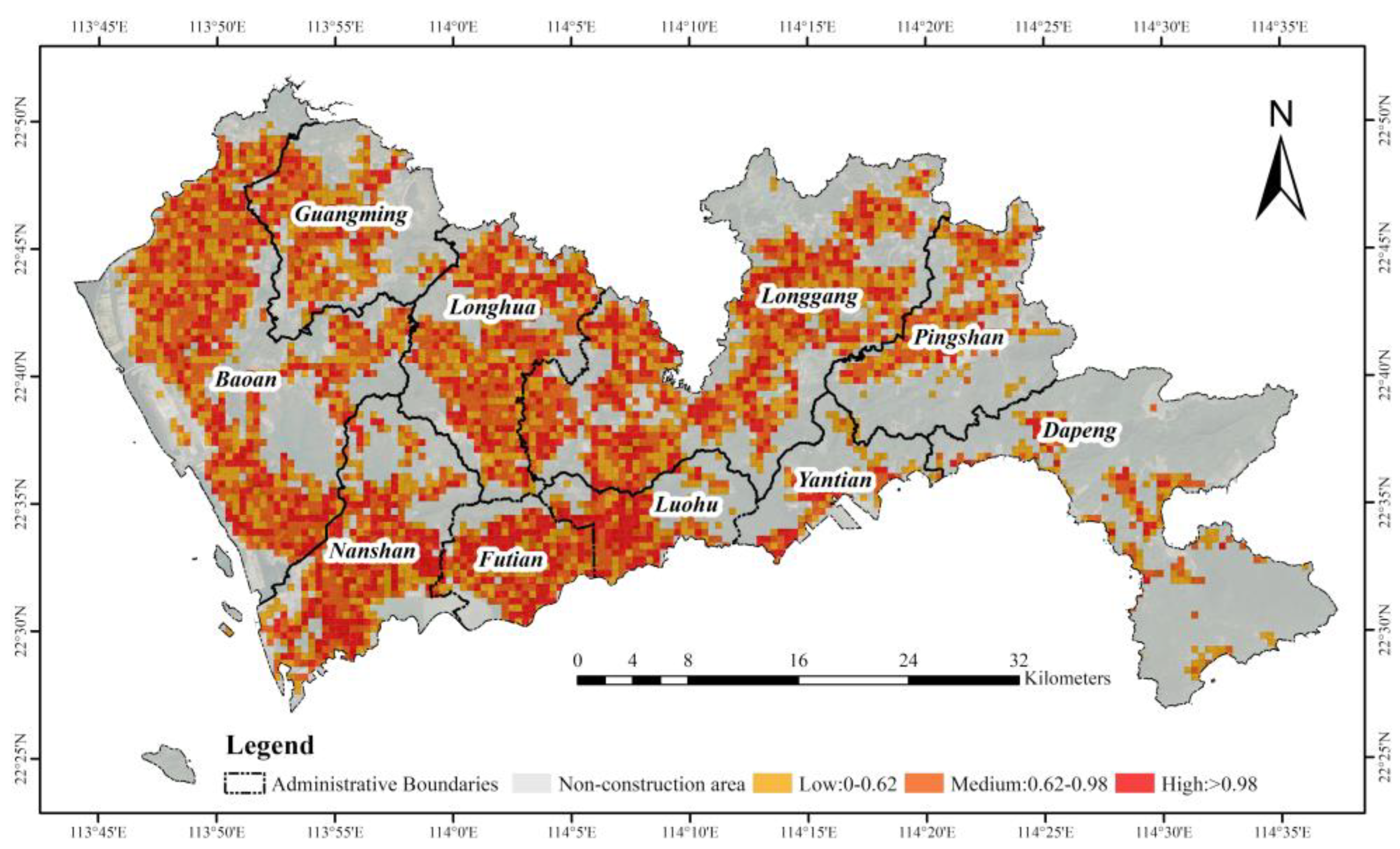
As Figure 5 shows, the mixed entropy (ME) of functional construction land in each grid was calculated and showed obvious spatial aggregation. The natural breaks (Jenks) method [76] was used to divide the mixing entropy values into three groups (0–0.62, 0.62–0.98, >0.98), representing the mixed degree of low, medium, and high, respectively. Most grids with a high mixed degree are concentrated in Futian, Luohu, Nanshan, and southern Baoan, which shows a similar distribution as grids of Business services function (B) and Street and transportation function (S).
In addition, the grids along the center of other districts are also with a high-level mixed degree, as it can be inferred that the grids with a high mixed degree are usually the regions with mature commercial activities and convenient traffic lines. Meanwhile, the grids with a medium mixed degree are mainly distributed in northern Baoan, Longhua, Pingshan, Longgang, and Yantian, where there is Manufacture function (M) and Residential function (R) grids are mainly distributed. Besides, the grids with a low mixed degree are mainly concentrated in mountainous areas, e.g., northern Yantian, Dapeng, and northern Nanshan, where there is less construction land but more ecological land (woodland and waterbody) distributed.

3.2. Differential Surface Temperature in FCLZs

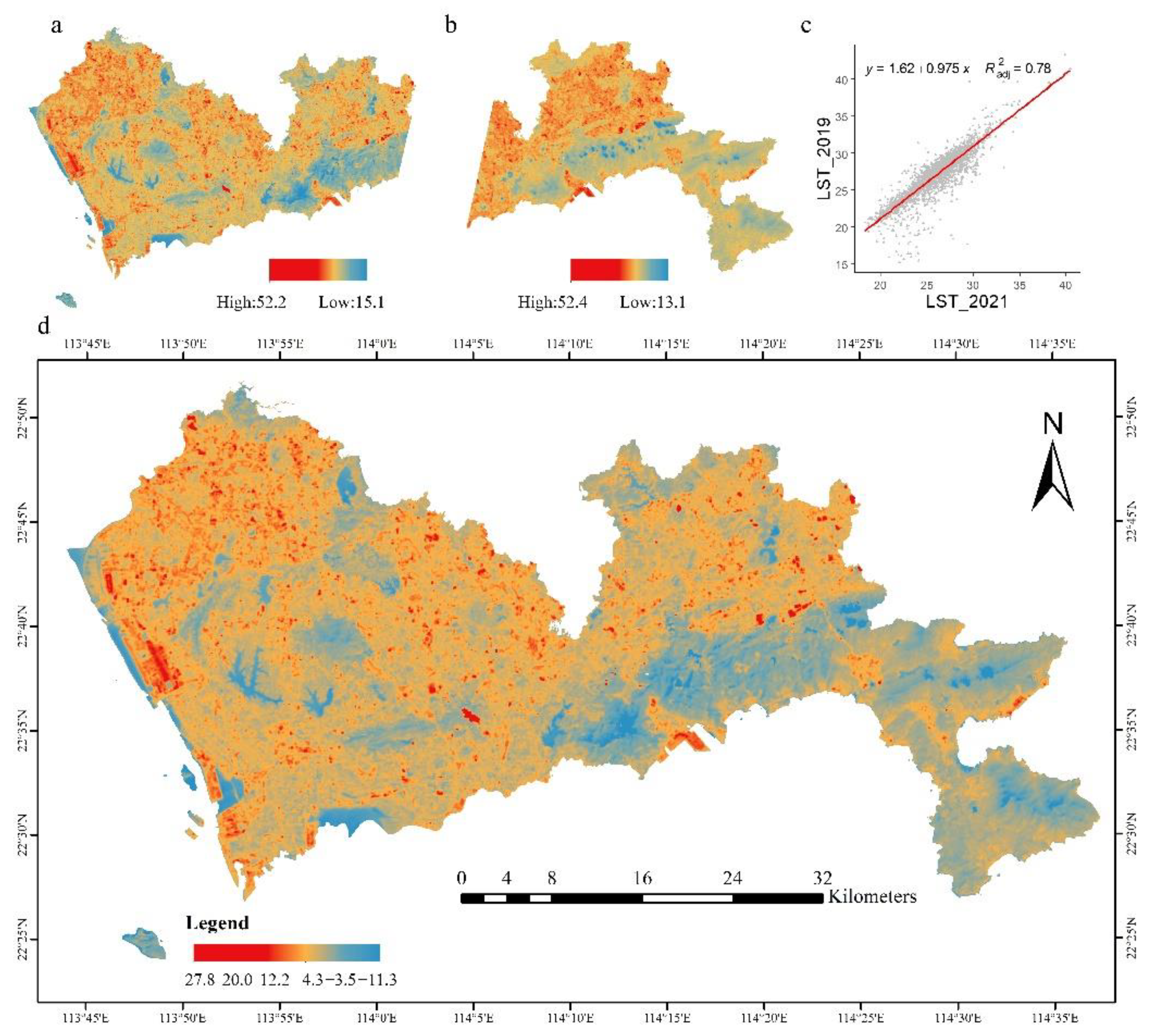
The LSTP images cannot cover the study area in a single scene due to the satellite orbits across both the two paths in different periods (Figure 6a,b), thus we scattered the retrieved LST values in the overlapping areas to find the relationship between them. The fitting curve and regression coefficient (Figure 6c) showed a high degree of linear consistency between the two images. Therefore, we finally obtained the DST data (Figure 6d) covering the whole area of Shenzhen computed based on mosaicking the two LST images after linear adjustment.
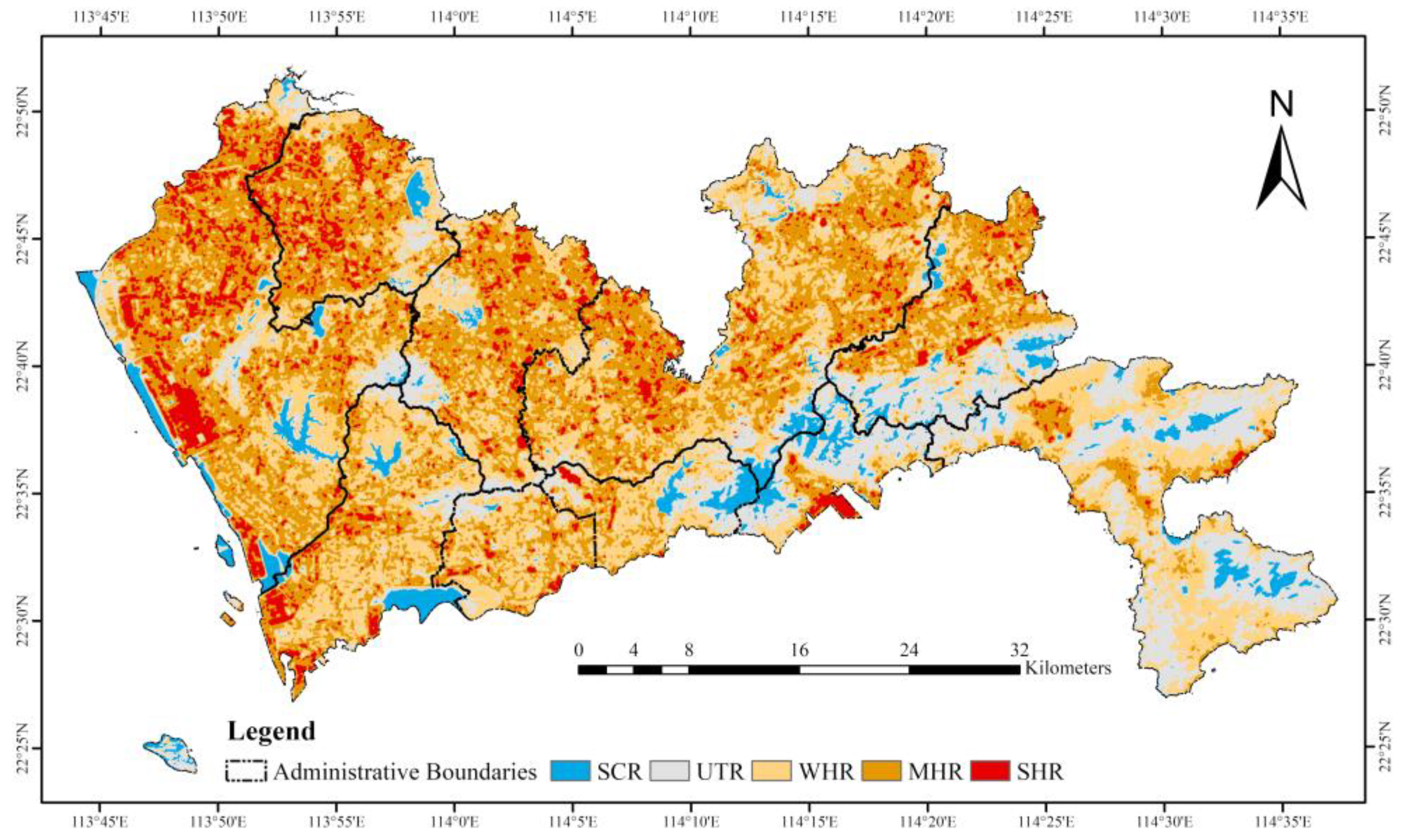
To reflect the DST difference in more detail, the mean-standard deviation method [77,78] was used to classify the DST data into five urban thermal effect levels, which correspond to the significant cooling effect region (SCR), the unnoticeable thermal difference region (UTR), the weak heat effect region (WHR), the moderate heat effect region (MHR), and the significant heat effect region (SHR) in Table 3 and Figure 7. It could be seen from the comparison between Figure 6 and Figure 7 that the regions with different levels of heat effect (WHR, MHR, and SHR) show a spatial distribution of high similarity to that of FCLZs. While SCR presents a spatial conjugate relationship to heat effect regions, UTR is mainly distributed in the mountainous woodland area and places adjacent to the waterbody areas.
Meanwhile, we calculated the area proportion of heat effect regions in both construction land and non-construction areas to explore the contribution of various types of FCLZs to the urban thermal environment. Results (Table 3) show that although it is clear that construction land contributes more to heat effect regions than non-construction areas, both the different degree of contribution between various FCLZs and the contribution from non-construction areas (at least >14.54%) cannot be ignored.
The Shapiro-Wilk test results (Table 4) show all DSTs in each functional construction land zone and non-construction areas were not statistically normal distributions except for functions G and R. The results of the Kruskal-Wallis H test and the multiple comparisons (Table 5) prove significant differences of DST among different FCLZs.
Although there were no significant differences in DST between functional land G and R, either W or M; it was significantly different for most pairs of construction land types. The above results indicate that the DST distribution in functional land G and R is similar to that in functional A, while the functional land W showed similar characteristics in DST of functional B, M, and S.

3.3. DST Relationships with Surface Environmental Indictors

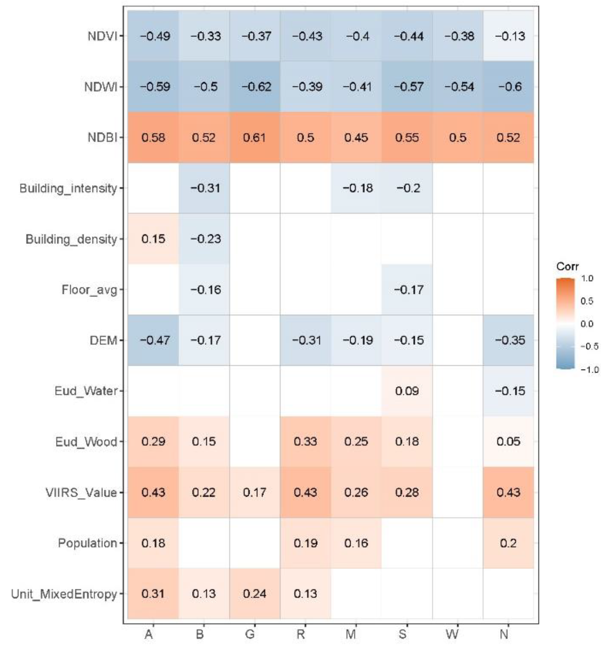
Figure 8 shows that the coefficients in functions A, G, and R are more consistent with non-construction areas while the building factors in function types B, M, S, and W present opposite effects to those in non-construction areas at a significant level of 0.05, which also supports the results in Table 5 from another quantitative perspective. Similar coefficients suggest similar relationships between DST to environmental indicators, while the different sizes of the coefficients indicate there are diversified differences in thermal capacity in construction land. Furthermore, according to the results of statistical differences (Table 5) and coefficients (Figure 8), we divided 7 types of construction land functional areas into 2 groups (group A, G, and R; group B, M, S, and W).
With different intercepts in the linear and approximate linear relationships between thermal responses of the three biophysical indicators to DST, it is found that the main differences are in the degree rather than the mode.
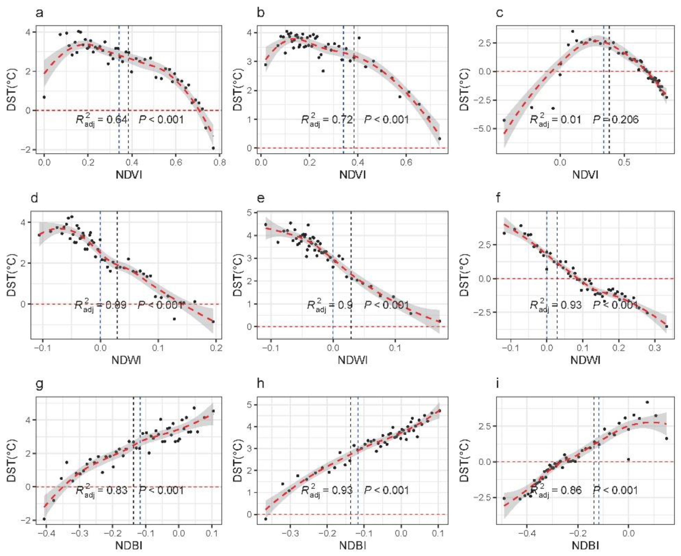
DST in two groups of FCLZs shows a downward trend on the whole (Figure 9a,b), even if an insignificant upward trend is shown when the NDVI value is small (<0.2). In the non-construction areas, the first-increase and then-decreasing trends are more obvious (Figure 9c). As for NDWI in both groups FCLZs and non-construction areas, a consistent linear decline appears simultaneously. Although the increase of NDWI reduces the size of DST in group B, M, S, and W, it is consistently found that the increase of NDWI cannot offset the warming effect (Figure 9e). While the cooling effect (DST < 0 °C) of NDWI is found both in the group for functions of A, G, and R and in non-construction areas when the values are larger than 0.15 and 0.1, respectively (Figure 9d,f). Similar findings are observed in the warming effect of NDBI. DST presents similar linear growing trends in both groups of FCLZs and the non-construction areas (Figure 9g–i) with the increase of NDBI. However, the same value of NDBI has different warming effects in the two groups, while in non-construction areas, the warming effect (DST > 0 °C) is coexisting with the cooling effect (DST > 0 °C) with a boundary value ~−0.25.
Figure 10 shows that the responses of DST to building indicators present different trends between the group of functions for A, G, and R and the group of functions for B, M, S, and W. The increases in Building_density and Building_intensity finally display stable warming effects with DST above 2.0 °C, however, the trends of curves indicate that intensifying and heightening buildings weaken the warm effects in the group of functions for B, M, S, and W (Figure 10b,e) but makes little significant contribution to the DST change in the group of function for A, G, and R (Figure 10a,d). A slight reduction of warming effects is also shown with the increase of Floor_avg in the group of functions for B, M, S, and W while in the group of functions for A, G, and R, the increase of Floor_avg leads to the DST increase first and then tends to be stable.
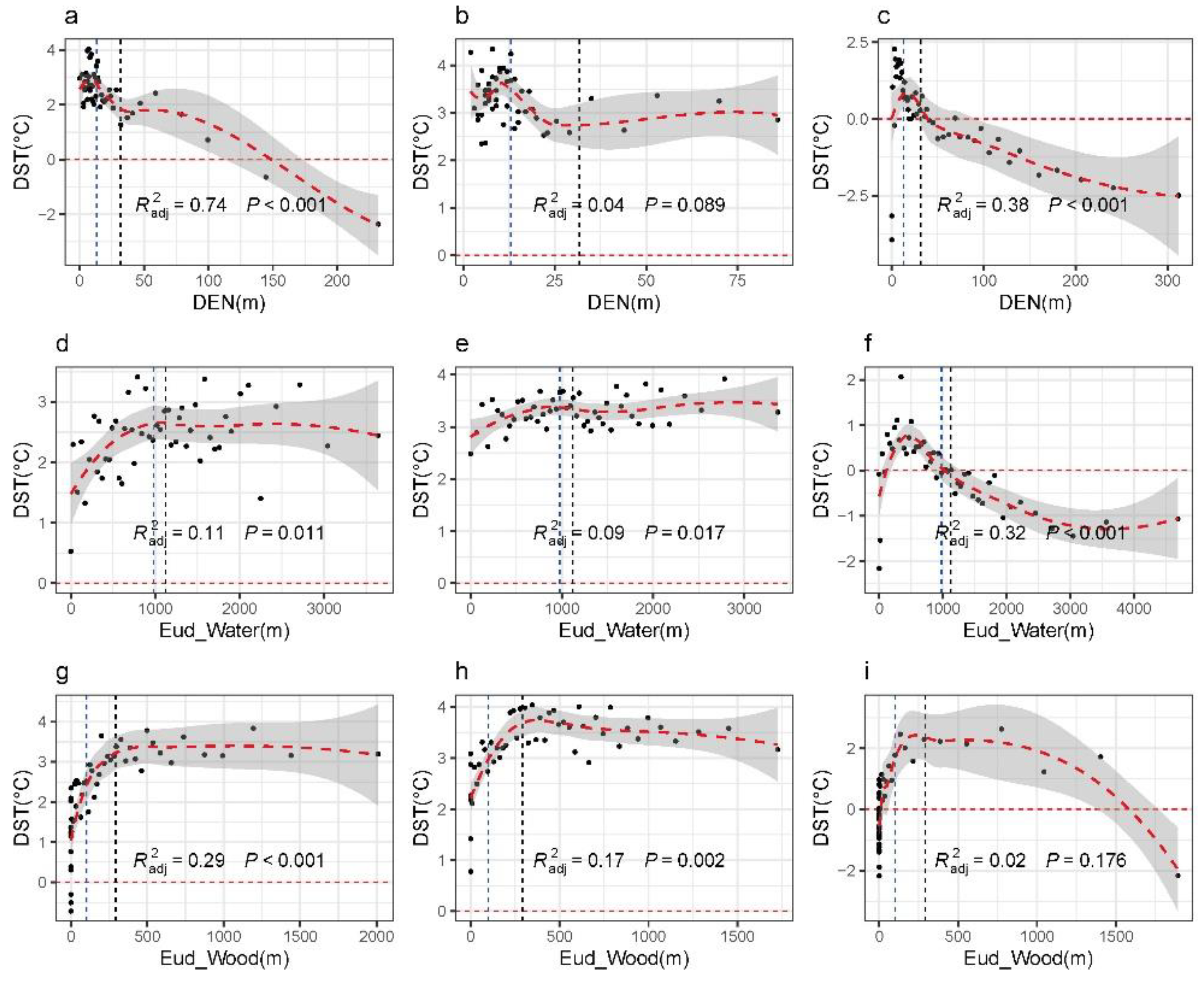
As is shown in Figure 11c, DST in the two groups both presents a short rising stage with the increase of elevation (DEM) before the altitude is less than average values (~25 m) and the cooling effect appears in the non-construction areas with the increase of DEM value. When the elevation is larger than median values (~30 m), the DST in the group of functions for A, G, and R shows a declining trend of warming effect and finally presents cooling effects when the elevation is larger than ~150 m. However, a stable state of warming effect at 2.75 °C after a rapid decline is also shown in the group of functions for B, M, S, and W.
The comparison of the other two location indicators (Eud_Water and Eud_Wood) represents the responses of DST to the distances from these two types of cooling areas. Different from the natural distance effects in non-construction areas (Figure 11f,i), DST increases then tend to be stable after different values as the increase of distance from cooling areas in different groups of FCLZs, showing that the limited spatial ranges of cooling effect are diversified (Figure 11d–h). Besides, the stable points of Eud_Water and Eud_Wood to the group functions for A, G, and R and B, M, S, and W are close to the median distances with values of ~1000 m and ~300 m, respectively.
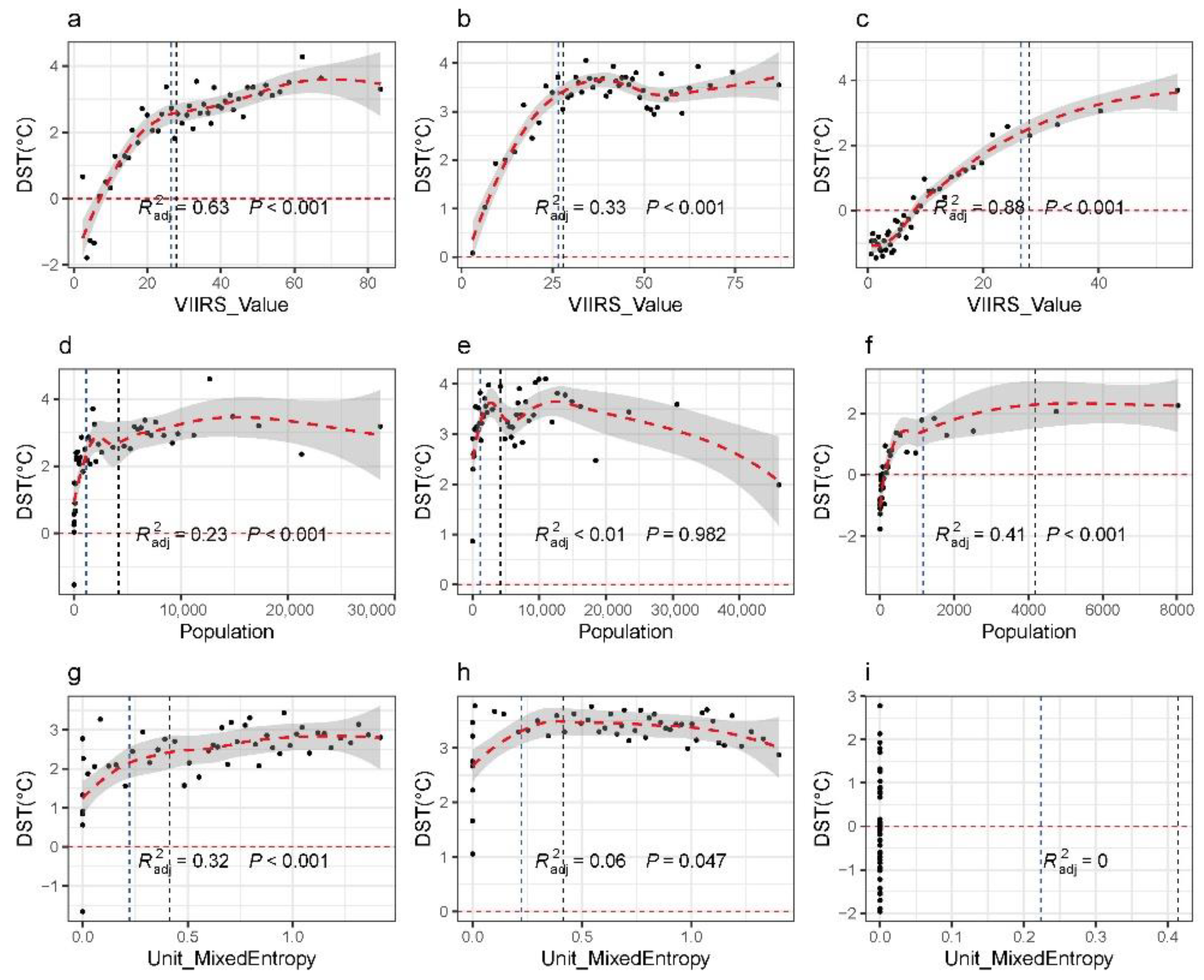
Further analysis revealed there is a saturation effect with similar trends in social-economic indicators like that with location indicators and the thresholds for saturation likewise varied between the groups of FCLZs (Figure 12). As with the increases of VIIRS_Value, DST increases at first and then tends to be stable below 4.0 °C for all FCLZs (Figure 12a,b) and in the non-construction areas, there is a linear increase trend (Figure 12c). The stable points are ~30 in the group of functions for B, M, S, and W, and ~60 in the group of functions for A, G, R. The increase in population (Figure 12d–f) would cause the warming effect to reach saturation points (3~4 °C for construction land and 2.5 °C for non-construction areas) at about 3000~5000 people per grid (0.25 square kilometers). Curves in Figure 12g,h indicate that even the same level of the mixed utilization of urban construction land (Unit_MixedEntropy) could lead to a stronger warming effect in FCLZs.

4. Discussion

4.1. Consistency Analysis of Recognized FCLZs

In this study, 4755 grids were identified as functional construction land zones and 3820 are non-construction areas (Figure 4). Comparing the total amount of construction land and manual discrimination of random samples could evaluate the effectiveness of recognized FCLZs quantitatively and qualitatively. Calculated with the functional proportion in each grid, the total area of functional construction land zones is 1171.1 square kilometers, of which the difference is 16.4% from the construction land area (1005.9 square kilometers) in the official report by the Planning and Natural Resources Bureau and Statistics Bureau of Shenzhen [51]. In addition, considering that the area of new construction land in 2019 was likely to increase according to the government’s land supply plan and development demands, the actual smaller difference suggests the method of FCLZs could measure the construction land total amount with relative quantity accuracy at a low cost and in a fast way. Moreover, the degree of mixed functional construction land zones in Shenzhen is closely related to the development status of the region, i.e., the higher the mixed degree of the grid indicates the more diverse human activities and land use patterns (Figure 5). Through random sampling and manual interpretation (Figure A1), we verified that different social-economic functions and the characteristic of mixed-use of construction land within the indistinguishable image features could be identified and reflected through FCLZs.
FCLZs map the attributes of POIs to the corresponding social function on a particular unit of space, which is different from land use and land cover types because the classification of construction land is more research-goal oriented due to the diversity and versatility of human activities in urban construction land. POIs or any other data with location information referring to functional land could be used and patches could be any spatial unit with valid meaning and shape besides grids or blocks. However, the grid size has a great influence on the final recognition result of urban functional land because the functional types of each grid unit are determined through the spatial distribution and quantities of POIs contained in each grid. Due to the limited number of POIs in real life, if the grid scale is too small or lower than the precision of the coordinates of POIs, the functional types inferred will not be meaningful due to collection errors. At the same time, too large a grid scale will make it difficult to show the transition and differences of regional changes in different types of functional construction land zones.

4.2. Differential Thermal Contribution in FCLZs

The non-parametric methods were used in the difference test, as the DST distributions in FCLZs except G and R followed left-skew distribution rather than a normal distribution [79]. FCLZs were divided into two groups according to the Dunn test (Table 5) and environmental indicators correlation validation (Figure 8), which indicates similarity and difference coexist in the thermal effects of urban construction land among various functional types. The results proved that the UHI is not only caused by construction land [66,80] but also has significant inner differences due to functions [70,79]. Although LCZ could divide the urban land through buildings and image characteristics [16], it lacks the detailed reflection of social-economic functions and is usually applied to study the problems caused by the physical environment in the heat island issues [14,15].
The thermal contribution proportions of different FCLZs are usually affected by the area size in terms of the total contribution, however, the thermal contribution at urban thermal effect levels is not completely consistent with the area. We found that the Business services function (B) contributes most with proportions of 32.63~43.96% to the considerable heat effect regions (MHR and SHR), which should be given priority in UHI control and mitigation in Shenzhen. Meanwhile, the non-construction areas (N) cannot be ignored, of which the contribution to WHR is 44.91%. All of the contribution proportions to heat effect regions for Street and transportation function (S), Manufacture function (M), and Warehousing and logistics function (W) increase rapidly from weak thermal effect to significant thermal effect.
DST between the FCLZs shows significantly different thermal capacity in construction land. The thermal difference in degrees among various FCLZs (Table 4) caused by social functions was measured. We found that the median thermal effects ranked from strong to weak are as follows: M (3.99 °C)> W (3.69 °C) > S (3.61 °C) > B (3.06 °C) > A (2.54 °C) > G (2.40 °C) > R (2.21 °C) > N (−0.06 °C), in which the ranks are similar to a case study conducted in Beijing [36] and thus it shows consistency in the degree of the thermal effect of social functions between cities in different climate zones [79]. In addition, it is noticeable that the minimum warming effect (R) is about 36.8 times that of non-construction areas in degrees, which indicates that regardless of the intensity and the way, the relative change of urban surface temperature induced by human activities is huge enough to increase hot extremes [81].

4.3. Differential Responses of DST to Environmental Indicators

Response processes of DST to environmental indicators have been key points to understand and regulate urban thermal effects. The indicators including the fraction of impervious surface have been discussed in previous studies [34,63,82], but the similarities and differences within construction land have not been clarified in detail. Our research investigated and refined the difference and consistency of various environmental indicators on DST in FCLZs. To further figure out the impacts of indicators on DST, we used the median resampled values to reduce random errors rather than the mean values because of the non-normality of DST data [79]. Equivalent repeated observation experiments were constructed by reorganizing the original grid-level data to ordered DST and corresponding indicator pairs. Scatter plots and single factor regression analyses were carried out on each pair of resampled values in the two groups of FCLZs with non-construction areas as the controlled group, to preliminarily explore the effect of each indicator on DST. On the whole, most of the indicators show similar trends but distinguished degrees of the effects on DST in the two groups, which proves that these indicators have similar effect modes [65] across the scale from a single city to global cities [26]. Non-linear relationships suggest the saturation effects exhibit in both distance and corresponding values of social-economic levels, for location indicators and social-economic indicators, respectively.

4.4. Potential Implication and Future Directions

This study investigated the thermal effects in construction land through a continuous division of social-economic functions at a 500-m grid-level using the FCLZs framework, which could extend the UHI analyses routine based on LUCC with more details about human-induced thermal contribution to the urban environment [10]. Our results show that urban heat island is not only mostly caused by the amount of different land use or land cover types, but there are also still significant differences within construction land induced by their social functions. Both similarities and differences exist in the responses to environmental indicators among FCLZs. Therefore, when the cooling capacities of GITs and [47,68,69] are insufficient or there are limits in maintaining and appropriately increasing green space and water bodies [27,68], except for controlling the expansion of urban areas [44], the relocation of the construction land with different social-economic functions and configuration with cooling and warming indicators at appropriate thresholds may be helpful ways to alleviate urban heat island problems.
The limitation of this work is that FCLZs do not have clear boundaries in reality because of fuzzy positions of POIs, and it is hard to get an absolute ground truth map to calculate a confusion matrix for absolute accuracy comparison. Random sampling for verification and comparison with official statics is the currently limited method to compare relative accuracy. Due to the different response processes among FCLZs, the tradeoff and synergies between environment indicators in construction should be the focus of future research.

5. Conclusions

This research established a general framework for functional construction land zones (FCLZs) mapping based on multi-sourced data to investigate their different contribution to the urban thermal environment in Shenzhen, China. The thermal environment is characterized by DST extracted from land surface temperature data. Based on the difference test of DST, FCLZs were then divided into groups of functions for A, G, and R and groups of functions for B, M, S, and W to analyze the thermal response with 12 environmental indicators considering surface biophysics, buildings, location, and social-economic development.
We found that: (1) The thermal effect and total contribution FCLZs are significantly different. Although construction land leads to an obvious warming effect with a median value of 2.94 °C in the urban environment, thermal contribution in FCLZs is significantly different. FCLZs contribute to MHR and SHR (moderate and significant heat regions) with a proportion of 82.63~85.46%, which highly exceeds the corresponding proportion in non-construction areas. As for weaker warming effect regions, the contribution of non-construction areas cannot be ignored because of the size (44.91%). The median thermal effects of various FCLZs are as follows: M (3.99 °C)> W (3.69 °C) > S (3.61 °C) > B (3.06 °C) > A (2.54 °C) > G (2.40 °C) > R (2.21 °C), and the minimum thermal warming effect of R is about 36.8 times than unnoticeable thermal effect (−0.06 °C) in the non-construction areas. (2) Difference and consistency coexist in responses of DST to various environmental indicators in FCLZs. Different intercepts in the consistent linear and approximate linear relationships indicated the differences between thermal responses of biophysical indicators (NDBI, NDVI, and NDWI) in FCLZs were mainly in degree rather than mode. Buildings indicators (Building_density, Building_intensity, and Floor_avg) showed weak inversed relationships with DST in the two groups. The saturation effects shown in response of DST to location (DEM, Eud_Water, and Eud_Wood) and social-economic indicators (Unit_MixedEnropy, VIIRS_Value, and Population) proved that distance and social-economic development contribute to the nonlinear change of urban thermal environment. The stable points for the two groups are ~1000 m and ~300 m, respectively, both of which are almost double the distances from the cooling region than the truing points in non-construction areas. Social-economic indicators would have no more impact on the thermal environment when reaching stable points.
It is an attempt to measure the differences in thermal environment in view of functional construction land zones. The findings of this research could extend the understanding of urban thermal warming mechanisms from the different social-economic activities reflected by the agent of FLCZs and provide new macroscopic perspectives on reducing the negative impacts of urban heat islands by combining scientific adjustment of environmental indicators according to their responses processes with the allocation of construction land in urban planning.

Author Contributions

Conceptualization, methodology, writing—original draft, visualization, writing—review and editing, H.W.; methodology, validation, writing—review and editing, B.L.; validation, writing—review and editing, T.Y.; formal analysis, supervision, funding acquisition, J.W. All authors have read and agreed to the published version of the manuscript.

Funding

This research was funded by Shenzhen Fundamental Research Program, grant number GXWD20201231165807007-20200816003026001.

Conflicts of Interest

The authors declare no conflict of interest.

Appendix A

Table A1. Reclassification system of POIs to functional construction land zones.
Functional ClassSub-Functional ClassClass CodeTag of POIs
Residential Function---RResidential community, villas, community centers
Administration and public services FunctionAdministrationA1Government agency, Industrial and commercial bureau, public security bureau, procuratorates, courts, democratic Parties, social organization, public institutions
Cultural facilitiesA2Public library, museum, science, and technology museum, art gallery, archives center, exhibition center, convention center
Education and research developmentA3Colleges and universities, technical secondary school, high school, middle school, primary school, research, and development institution
SportsA4Gymnasium, court, sports training sites
Medical Treatment and Public HealthA5Health care services, general hospital, specialized hospital, clinic, emergency center, disease prevention agency
Public welfareA6Welfare house, nursing home, orphanage
Conservation of historic landmarks and sitesA7Scenic spots and historical sites, tourist attractions, revolutionary site
Religious facilitiesA9Church, mosque, temple
Business
Services Function
(B)
Commercial FacilitiesB1Retail business (shopping malls, supermarkets, shops, etc.)
Wholesale market
Catering services (restaurant, bar, tea house, cake shop, cafe, cold drink, and dessert shop)
Accommodation services (hotels, guest houses, and resorts)
Business FacilitiesB2Financial insurance (banking and insurance company, ATM, securities company, financial and insurance service organization)
Art Media (Media organizations such as music, fine arts, film, television, advertising, network media, art groups)
Other business facilities companies
Recreation facilitiesB3Entertainment facilities (theatre, concert hall, cinema, song, dance hall, Internet cafe, amusement park)
Recreation and Sports facilities (Golf Driving Range Racecourse Skating Rink Skydiving Range Motorcycle Range Shooting Range)
Public utilitiesB4Refueling and filling stations (refueling and filling stations and other energy stations)
Public facilities business outlets (telecommunications, postal service, water supply, gas supply, heat supply, etc.)
OthersB9Scientific, educational and cultural services (training institutions) medical and health services (clinics, medical and health sales shops, animal medical places) automobile services life services funeral services
Green spaces and squares (G)park green spaceG1Park, zoo, botanical garden
street and square green areaG3City square
Street and transport function
(S)
Transport hubS3Railway station, long distance bus station, port and pier
Transport stationsS4Transport facilities (car parks, bus stops, MTR stations)
OthersS9Car training ground
Manufacture Function
(M)
----Industrial park, factory
Warehousing and logistics Function (W)----Logistics warehouse
Figure A1. Random sampling grids for functional construction land zones manual verification.
Remotesensing 14 01851 g0a1

References

  1. Kalnay, E.; Cai, M. Impact of urbanization and land-use change on climate. Nature 2003, 423, 528–531. [Google Scholar] [CrossRef] [PubMed]
  2. Deng, J.S.; Wang, K.; Hong, Y.; Qi, J.G. Spatio-temporal dynamics and evolution of land use change and landscape pattern in response to rapid urbanization. Landsc. Urban Plan. 2009, 92, 187–198. [Google Scholar] [CrossRef]
  3. Sun, L.; Chen, J.; Li, Q.; Huang, D. Dramatic uneven urbanization of large cities throughout the world in recent decades. Nat. Commun. 2020, 11, 5366. [Google Scholar] [CrossRef] [PubMed]
  4. Ritchie, H.; Roser, M. Urbanization. Available online: https://ourworldindata.org/urbanization (accessed on 25 June 2021).
  5. Peng, S.; Piao, S.; Ciais, P.; Friedlingstein, P.; Ottle, C.; Bréon, F.M.; Nan, H.; Zhou, L.; Myneni, R.B. Surface urban heat island across 419 global big cities. Environ. Sci. Technol. 2012, 46, 696–703. [Google Scholar] [CrossRef] [PubMed]
  6. Manoli, G.; Fatichi, S.; Schläpfer, M.; Yu, K.; Crowther, T.W.; Meili, N.; Burlando, P.; Katul, G.G.; Bou-Zeid, E. Magnitude of urban heat islands largely explained by climate and population. Nature 2019, 573, 55–60. [Google Scholar] [CrossRef] [PubMed]
  7. Tomlinson, C.J.; Chapman, L.; Thornes, J.E.; Baker, C.J. Including the urban heat island in spatial heat health risk assessment strategies: A case study for Birmingham, UK. Int. J. Health Geogr. 2011, 10, 42. [Google Scholar] [CrossRef] [PubMed] [Green Version]
  8. Estoque, R.C.; Ooba, M.; Seposo, X.T.; Togawa, T.; Hijioka, Y.; Takahashi, K.; Nakamura, S. Heat health risk assessment in Philippine cities using remotely sensed data and social-ecological indicators. Nat. Commun. 2020, 11, 1581. [Google Scholar] [CrossRef] [Green Version]
  9. Ravanelli, R.; Nascetti, A.; Cirigliano, R.V.; Di Rico, C.; Leuzzi, G.; Monti, P.; Crespi, M. Monitoring the impact of land cover change on surface urban heat island through Google Earth Engine: Proposal of a global methodology, first applications and problems. Remote Sens. 2018, 10, 1488. [Google Scholar] [CrossRef] [Green Version]
  10. Dong, J.; Peng, J.; He, X.; Corcoran, J.; Qiu, S.; Wang, X. Heatwave-induced human health risk assessment in megacities based on heat stress-social vulnerability-human exposure framework. Landsc. Urban Plan. 2020, 203, 103907. [Google Scholar] [CrossRef]
  11. Coseo, P.; Larsen, L. How factors of land use/land cover, building configuration, and adjacent heat sources and sinks explain Urban Heat Islands in Chicago. Landsc. Urban Plan. 2014, 125, 117–129. [Google Scholar] [CrossRef]
  12. Zhou, D.; Zhao, S.; Liu, S.; Zhang, L.; Zhu, C. Surface urban heat island in China’s 32 major cities: Spatial patterns and drivers. Remote Sens. Environ. 2014, 152, 51–61. [Google Scholar] [CrossRef]
  13. Lin, P.; Lau, S.S.Y.; Qin, H.; Gou, Z. Effects of urban planning indicators on urban heat island: A case study of pocket parks in high-rise high-density environment. Landsc. Urban Plan. 2017, 168, 48–60. [Google Scholar] [CrossRef]
  14. Stewart, I.D.; Oke, T.R. Local climate zones for urban temperature studies. Bull. Am. Meteorol. Soc. 2012, 93, 1879–1900. [Google Scholar] [CrossRef]
  15. Bechtel, B.; Alexander, P.J.; Böhner, J.; Ching, J.; Conrad, O.; Feddema, J.; Mills, G.; See, L.; Stewart, I. Mapping local climate zones for a worldwide database of the form and function of cities. ISPRS Int. J. Geo-Inf. 2015, 4, 199–219. [Google Scholar] [CrossRef] [Green Version]
  16. Quan, J. Multi-temporal effects of urban forms and functions on urban heat islands based on local climate zone classification. Int. J. Environ. Res. Public Health 2019, 16, 2140. [Google Scholar] [CrossRef] [Green Version]
  17. Liu, S.; Shi, Q. Local climate zone mapping as remote sensing scene classification using deep learning: A case study of metropolitan China. ISPRS J. Photogramm. Remote Sens. 2020, 164, 229–242. [Google Scholar] [CrossRef]
  18. Zhao, C.; Jensen, J.L.R.; Weng, Q.; Currit, N.; Weaver, R. Use of Local Climate Zones to investigate surface urban heat islands in Texas. GISci. Remote Sens. 2020, 57, 1083–1101. [Google Scholar] [CrossRef]
  19. Zhou, X.; Okaze, T.; Ren, C.; Cai, M.; Ishida, Y.; Watanabe, H.; Mochida, A. Evaluation of urban heat islands using local climate zones and the influence of sea-land breeze. Sustain. Cities Soc. 2020, 55, 102060. [Google Scholar] [CrossRef]
  20. Yu, Z.; Jing, Y.; Yang, G.; Sun, R. A new urban functional zone-based climate zoning system for urban temperature study. Remote Sens. 2021, 13, 1–17. [Google Scholar] [CrossRef]
  21. Sun, R.H.; Lü, Y.; Chen, L.D.; Yang, L.; Chen, A.L.; Lu, Y.H.; Chen, L.D.; Yang, L.; Chen, A.L. Assessing the stability of annual temperatures for different urban functional zones. Build. Environ. 2013, 65, 90–98. [Google Scholar] [CrossRef]
  22. Liu, Y.; Peng, J.; Wang, Y. Relationship between urban heat island and landscape patterns: From city size and landscape composition to spatial configuration. Acta Ecol. Sin. 2017, 37, 7769–7780. [Google Scholar] [CrossRef]
  23. Yan, J.; Zhou, W.; Jenerette, G.D. Testing an energy exchange and microclimate cooling hypothesis for the effect of vegetation configuration on urban heat. Agric. For. Meteorol. 2019, 279, 107666. [Google Scholar] [CrossRef]
  24. Wang, J.; Meng, B.; Fu, D.; Pei, T.; Xu, C. Mapping spatiotemporal patterns and multi-perspective analysis of the surface urban heat islands across 32 major cities in China. ISPRS Int. J. Geo-Inf. 2018, 7, 207. [Google Scholar] [CrossRef] [Green Version]
  25. Sun, F.; Liu, M.; Wang, Y.; Wang, H.; Che, Y. The effects of 3D architectural patterns on the urban surface temperature at a neighborhood scale: Relative contributions and marginal effects. J. Clean. Prod. 2020, 258, 120706. [Google Scholar] [CrossRef]
  26. Yang, Q.; Huang, X.; Yang, J.; Liu, Y. The relationship between land surface temperature and artificial impervious surface fraction in 682 global cities: Spatiotemporal variations and drivers. Environ. Res. Lett. 2021, 16, 24032. [Google Scholar] [CrossRef]
  27. Bartesaghi-Koc, C.; Osmond, P.; Peters, A. Quantifying the seasonal cooling capacity of ‘green infrastructure types’ (GITs): An approach to assess and mitigate surface urban heat island in Sydney, Australia. Landsc. Urban Plan. 2020, 203, 103893. [Google Scholar] [CrossRef]
  28. Nakayama, T.; Fujita, T. Cooling effect of water-holding pavements made of new materials on water and heat budgets in urban areas. Landsc. Urban Plan. 2010, 96, 57–67. [Google Scholar] [CrossRef]
  29. Kotharkar, R.; Bagade, A. Evaluating urban heat island in the critical local climate zones of an Indian city. Landsc. Urban Plan. 2018, 169, 92–104. [Google Scholar] [CrossRef]
  30. Georgescu, M.; Morefield, P.E.; Bierwagen, B.G.; Weaver, C.P. Urban adaptation can roll back warming of emerging megapolitan regions. Proc. Natl. Acad. Sci. USA 2014, 111, 2909–2914. [Google Scholar] [CrossRef] [Green Version]
  31. Zhang, Y.; Murray, A.T.; Turner, B.L. Optimizing green space locations to reduce daytime and nighttime urban heat island effects in Phoenix, Arizona. Landsc. Urban Plan. 2017, 165, 162–171. [Google Scholar] [CrossRef]
  32. Andrade, R.; Alves, A.; Bento, C. Exploring different combinations of data and methods for urban land use analysis: A survey. In Proceedings of the 2019 Joint Poster and Workshop Sessions of AmI, AmI 2019 and 2019 European Conference on Ambient Intelligence, Rome, Italy, 13–15 November 2019; Strinati, E.C., Charitos, D., Chatzigiannakis, I., Ciampolini, P., Cuomo, F., Di Lorenzo, P., Gavalas, D., Hanke, S., Komninos, A., Mylonas, G., Eds.; CEUR-WS: Aachen, Germany, 2019; Volume 2492, pp. 55–65. [Google Scholar]
  33. Niu, H.; Silva, E.A. Crowdsourced Data Mining for Urban Activity: Review of Data Sources, Applications, and Methods. J. Urban Plan. Dev. 2020, 146, 04020007. [Google Scholar] [CrossRef] [Green Version]
  34. Feng, Y.; Du, S.; Myint, S.W.; Shu, M. Do urban functional zones affect land surface temperature differently? A case study of Beijing, China. Remote Sens. 2019, 11, 1802. [Google Scholar] [CrossRef] [Green Version]
  35. Huang, X.; Wang, Y. Investigating the effects of 3D urban morphology on the surface urban heat island effect in urban functional zones by using high-resolution remote sensing data: A case study of Wuhan, Central China. ISPRS J. Photogramm. Remote Sens. 2019, 152, 119–131. [Google Scholar] [CrossRef]
  36. Li, T.; Cao, J.F.; Xu, M.X.; Wu, Q.Y.; Yao, L. The influence of urban spatial pattern on land surface temperature for different functional zones. Landsc. Ecol. Eng. 2020, 16, 249–262. [Google Scholar] [CrossRef]
  37. Liu, X.; Long, Y. Automated identification and characterization of parcels with OpenStreetMap and points of interest. Environ. Plan. B Plan. Des. 2016, 43, 341–360. [Google Scholar] [CrossRef]
  38. Zhang, Y.; Li, Q.; Tu, W.; Mai, K.; Yao, Y.; Chen, Y. Functional urban land use recognition integrating multi-source geospatial data and cross-correlations. Comput. Environ. Urban Syst. 2019, 78, 101374. [Google Scholar] [CrossRef]
  39. Amap. Web Service API Related Downloads. POI Classification Code. Available online: https://a.amap.com/lbs/static/amap_3dmap_lite/amap_poicode.zip (accessed on 15 December 2021).
  40. Baidu. LBS. Cloud Service. POITags. Available online: https://lbsyun.baidu.com/index.php?title=lbscloud/poitags (accessed on 15 December 2021).
  41. Google Maps Platform. Places API. Place Types. Available online: https://developers.google.com/maps/documentation/places/web-service/supported_types (accessed on 15 December 2021).
  42. Liu, H.; Xu, Y.; Tang, J.; Deng, M.; Huang, J.; Yang, W.; Wu, F. Recognizing urban functional zones by a hierarchical fusion method considering landscape features and human activities. Trans. GIS 2020, 24, 1359–1381. [Google Scholar] [CrossRef]
  43. Wu, J.; Li, S.; Shen, N.; Zhao, Y.; Cui, H. Construction of cooling corridors with multiscenarios on urban scale: A case study of Shenzhen. Sustainability 2020, 12, 5903. [Google Scholar] [CrossRef]
  44. Qian, J.; Peng, Y.; Luo, C.; Wu, C.; Du, Q. Urban land expansion and sustainable land use policy in Shenzhen: A case study of China’s rapid urbanization. Sustainability 2016, 8, 16. [Google Scholar] [CrossRef] [Green Version]
  45. Cao, J.; Zhou, W.; Zheng, Z.; Ren, T.; Wang, W. Within-city spatial and temporal heterogeneity of air temperature and its relationship with land surface temperature. Landsc. Urban Plan. 2021, 206, 103979. [Google Scholar] [CrossRef]
  46. Wu, J.; Li, C.; Zhang, X.; Zhao, Y.; Liang, J.; Wang, Z. Seasonal variations and main influencing factors of the water cooling islands effect in Shenzhen. Ecol. Indic. 2020, 117, 106699. [Google Scholar] [CrossRef]
  47. Peng, J.; Dan, Y.; Qiao, R.; Liu, Y.; Dong, J.; Wu, J. How to quantify the cooling effect of urban parks? Linking maximum and accumulation perspectives. Remote Sens. Environ. 2021, 252, 112135. [Google Scholar] [CrossRef]
  48. Amap. Guides for Developers: API Documents for Serarching POI. Available online: https://lbs.amap.com/api/webservice/guide/api/search/ (accessed on 15 March 2019).
  49. Kristi, S. Landsat 8 Collection 2 (C2) Level 2 Science Product (L2SP) Guide. Available online: https://www.usgs.gov/media/files/landsat-8-collection-2-level-2-science-product-guide (accessed on 8 October 2021).
  50. Ministry of Natural Resources. Globeland30: Global Geo-Information Public Product. Available online: http://www.globallandcover.com/ (accessed on 13 May 2021).
  51. Shenzhen Municipal Bureau of Planning and Natural Resources; Shenzhen Municipal Bureau of Statistics. Report of the Main Data Results of Shenzhen Land Change Survey in 2018. Available online: http://pnr.sz.gov.cn/xxgk/sjfb/tjsj/content/post_7058772.html (accessed on 20 April 2021).
  52. Geospatial Data Cloud Digital Elevation Data of GDEMV2 30M. Available online: https://www.gscloud.cn/sources/accessdata/421?pid=302 (accessed on 14 May 2021).
  53. Earth Observation Group EOG Nighttime Light. Available online: https://eogdata.mines.edu/nighttime_light/annual/v20/ (accessed on 27 May 2021).
  54. Rose, A.N.; McKee, J.J.; Sims, K.M.; Bright, E.A.; Reith, A.E.; Urban, M.L. LandScan. 2019. Available online: https://landscan.ornl.gov/ (accessed on 27 May 2021).
  55. Liu, X.; Andris, C.; Rahimi, S. Place niche and its regional variability: Measuring spatial context patterns for points of interest with representation learning. Comput. Environ. Urban Syst. 2019, 75, 146–160. [Google Scholar] [CrossRef]
  56. Liu, K.; Yin, L.; Lu, F.; Mou, N. Visualizing and exploring POI configurations of urban regions on POI-type semantic space. Cities 2020, 99, 102610. [Google Scholar] [CrossRef]
  57. Ministry of Housing and Urban-Rural Development (MOHURD). Code for Classification of Urban Land Use and Planning Standards of Development Land; China Architecture & Building Press: Beijing, China, 2011; pp. 1–60.
  58. Kang, Y.; Wang, Y.; Xia, Z.; Chi, J.; Jiao, L.; Wei, Z. Identification and classification of Wuhan urban districts based on POI. J. Geomat. 2018, 43, 81–85. [Google Scholar] [CrossRef]
  59. Ramos, J. Using TF-IDF to Determine Word Relevance in Document Queries. In Proceedings of the first instructional conference on machine learning, Piscataway, NJ, USA, 3–8 December 2003; Volume 242, pp. 29–48. [Google Scholar]
  60. Malakar, N.K.; Hulley, G.C.; Hook, S.J.; Laraby, K.; Cook, M.; Schott, J.R. An Operational Land Surface Temperature Product for Landsat Thermal Data: Methodology and Validation. IEEE Trans. Geosci. Remote Sens. 2018, 56, 5717–5735. [Google Scholar] [CrossRef]
  61. Cook, M.; Schott, J.R.; Mandel, J.; Raqueno, N. Development of an operational calibration methodology for the Landsat thermal data archive and initial testing of the atmospheric compensation component of a land surface temperature (LST) product from the archive. Remote Sens. 2014, 6, 11244–11266. [Google Scholar] [CrossRef] [Green Version]
  62. Pettorelli, N.; Vik, J.O.; Mysterud, A.; Gaillard, J.M.; Tucker, C.J.; Stenseth, N.C. Using the satellite-derived NDVI to assess ecological responses to environmental change. Trends Ecol. Evol. 2005, 20, 503–510. [Google Scholar] [CrossRef]
  63. Wang, Y.; Yi, G.; Zhou, X.; Zhang, T.; Bie, X.; Li, J.; Ji, B. Spatial distribution and influencing factors on urban land surface temperature of twelve megacities in China from 2000 to 2017. Ecol. Indic. 2021, 125, 107533. [Google Scholar] [CrossRef]
  64. Hu, Y.; Dai, Z.; Guldmann, J.M. Modeling the impact of 2D/3D urban indicators on the urban heat island over different seasons: A boosted regression tree approach. J. Environ. Manag. 2020, 266, 110424. [Google Scholar] [CrossRef] [PubMed]
  65. Silva, A.G.L.; Torres, M.C.A. Proposing an effective and inexpensive tool to detect urban surface temperature changes associated with urbanization processes in small cities. Build. Environ. 2021, 192, 107634. [Google Scholar] [CrossRef]
  66. Li, Y.; Schubert, S.; Kropp, J.P.; Rybski, D. On the influence of density and morphology on the Urban Heat Island intensity. Nat. Commun. 2020, 11, 2647. [Google Scholar] [CrossRef] [PubMed]
  67. Yang, J.; Menenti, M.; Wu, Z.; Wong, M.S.; Abbas, S.; Xu, Y.; Shi, Q. Assessing the impact of urban geometry on surface urban heat island using complete and nadir temperatures. Int. J. Climatol. 2021, 41, E3219–E3238. [Google Scholar] [CrossRef]
  68. Li, X.; Zhou, W. Optimizing urban greenspace spatial pattern to mitigate urban heat island effects: Extending understanding from local to the city scale. Urban For. Urban Green. 2019, 41, 255–263. [Google Scholar] [CrossRef]
  69. Peng, J.; Liu, Q.; Xu, Z.; Lyu, D.; Du, Y.; Qiao, R.; Wu, J. How to effectively mitigate urban heat island effect? A perspective of waterbody patch size threshold. Landsc. Urban Plan. 2020, 202, 103873. [Google Scholar] [CrossRef]
  70. Liang, Z.; Wu, S.; Wang, Y.; Wei, F.; Huang, J.; Shen, J.; Li, S. The relationship between urban form and heat island intensity along the urban development gradients. Sci. Total Environ. 2020, 708, 135011. [Google Scholar] [CrossRef]
  71. Zhang, J.; Yuan, X.D.; Lin, H. The Extraction of Urban Built-Up Areas by Integrating Night-Time Light and POI Data-A Case Study of Kunming, China. IEEE Access 2021, 9, 22417–22429. [Google Scholar] [CrossRef]
  72. Royston, P. Approximating the Shapiro-Wilk W-test for non-normality. Stat. Comput. 1992, 2, 117–119. [Google Scholar] [CrossRef]
  73. Vargha, A.; Delaney, H.D. The Kruskal-Wallis Test and Stochastic Homogeneity. J. Educ. Behav. Stat. 1998, 23, 170–192. [Google Scholar] [CrossRef]
  74. Sture Holm A Simple Sequentially Rejective Multiple Test Procedure. Scand. J. Stat. 1979, 6, 65–70.
  75. De Winter, J.C.F.; Gosling, S.D.; Potter, J. Comparing the pearson and spearman correlation coefficients across distributions and sample sizes: A tutorial using simulations and empirical data. Psychol. Methods 2016, 21, 273–290. [Google Scholar] [CrossRef]
  76. Chen, J.; Yang, S.; Li, H.; Zhang, B.; Lv, J. Research on geographical environment unit division based on the method of natural breaks (Jenks). Int. Arch. Photogramm. Remote Sens. Spat. Inf. Sci. ISPRS Arch. 2013, 40, 47–50. [Google Scholar] [CrossRef] [Green Version]
  77. Chen, S.; Wang, T. Comparison Analyses of Equal Interval Method and Mean-standard Deviation Method Used to Delimitate Urban Heat Island. Geo-Inf. Sci. 2009, 11, 145–150. [Google Scholar] [CrossRef]
  78. Qiao, Z.; Sun, Z.; Sun, X.; Xu, X.; Yang, J. Prediction and analysis of urban thermal environment risk and its spatio- temporal pattern. Shengtai Xuebao/Acta Ecol. Sin. 2019, 39, 649–659. [Google Scholar] [CrossRef]
  79. Li, N.; Yang, J.; Qiao, Z.; Wang, Y.; Miao, S. Urban thermal characteristics of local climate zones and their mitigation measures across cities in different climate zones of China. Remote Sens. 2021, 13, 1468. [Google Scholar] [CrossRef]
  80. Huang, Q.; Huang, J.; Yang, X.; Fang, C.; Liang, Y. Quantifying the seasonal contribution of coupling urban land use types on Urban Heat Island using Land Contribution Index: A case study in Wuhan, China. Sustain. Cities Soc. 2019, 44, 666–675. [Google Scholar] [CrossRef]
  81. Liao, W.; Li, D.; Malyshev, S.; Shevliakova, E.; Zhang, H.; Liu, X. Amplified Increases of Compound Hot Extremes Over Urban Land in China. Geophys. Res. Lett. 2021, 48, e2020GL091252. [Google Scholar] [CrossRef]
  82. Shi, Y.; Liu, S.; Yan, W.; Zhao, S.; Ning, Y.; Peng, X.; Chen, W.; Chen, L.; Hu, X.; Fu, B.; et al. Influence of landscape features on urban land surface temperature: Scale and neighborhood effects. Sci. Total Environ. 2021, 771, 145381. [Google Scholar] [CrossRef]
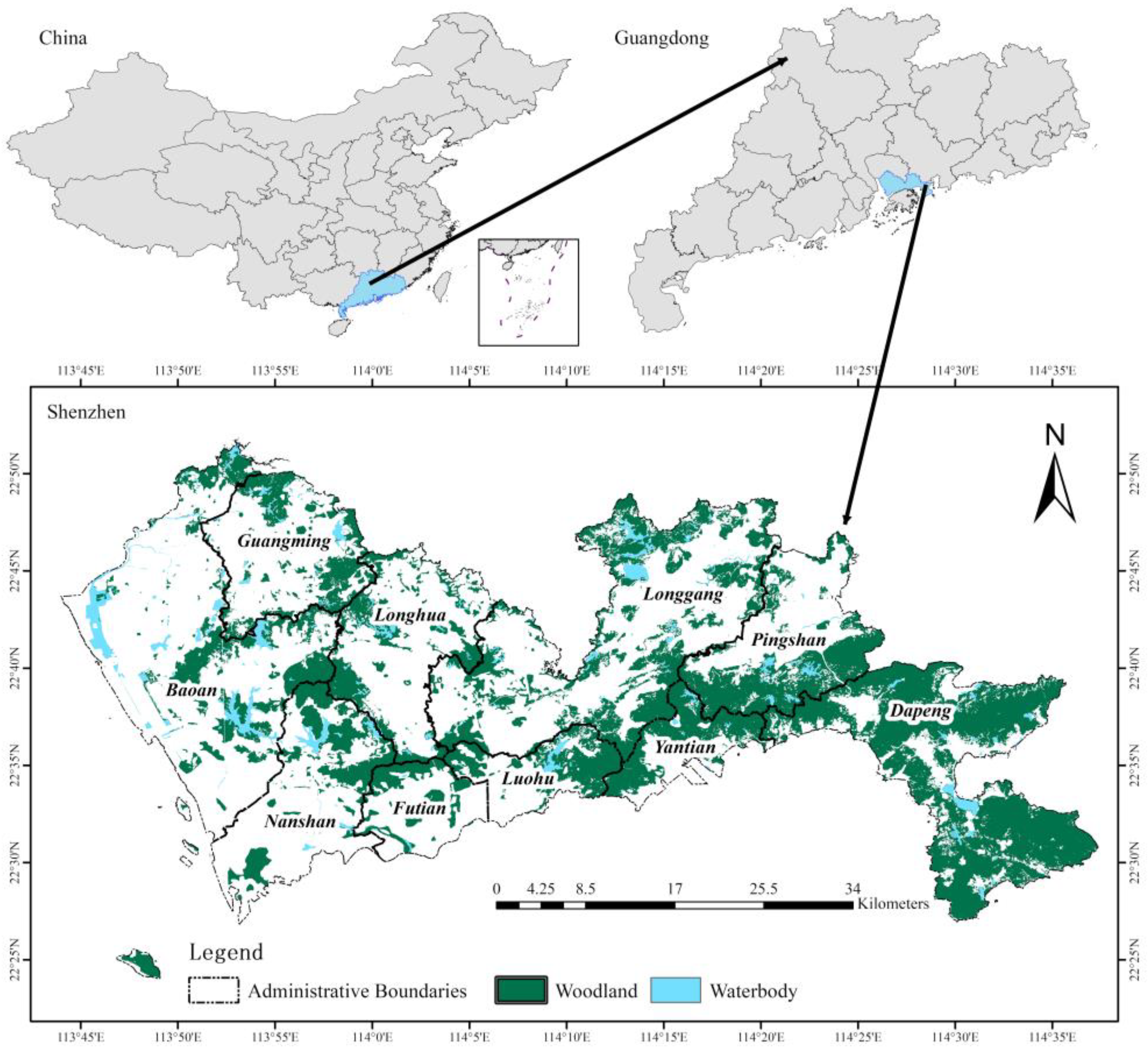
Figure 1. Location of Shenzhen: limited hilly woodland and waterbody distribution in the city.
Remotesensing 14 01851 g001
Figure 2. The research framework of heterogeneous thermal contribution analysis in urban construction areas.
Remotesensing 14 01851 g002
Figure 3. Patches diagrams in continuous grids (left) and road level blocks (right).
Remotesensing 14 01851 g003
Figure 4. The main type of functional construction land zone recognition results at a 500 m grid scale. A: Administration and public services function; B: Business services function; G: Green spaces and squares function; S: Street and transportation function; M: Manufacture function; R: Residential function; W: Warehousing and logistics function.
Remotesensing 14 01851 g004
Figure 5. Mixed entropy distribution of functional construction land zones at 500 m grid scale.
Remotesensing 14 01851 g005
Figure 6. Urban surface temperature results in Shenzhen. (a) land surface temperature retrieved from scene LC81220442021035LGN00; (b) land surface temperature retrieved from scene LC81210442019071LGN00; (c) scatter plot and regression between (land surface temperature) LST of the overlap region in 2019 and 2021. (d) Distribution of differential surface temperature (DST)(°C).
Remotesensing 14 01851 g006
Figure 7. Thermal effect levels distribution in Shenzhen. SCR: significant cooling effect region; UTR: unnoticeable thermal difference region; WHR: weak heat effect region; MFR: moderate heat effect region; SHR: significant heat effect region.
Remotesensing 14 01851 g007
Figure 8. Spearman correlation coefficients of DST with 12 biophysical and social-economic indicators in seven types of functional construction land zones and non-construction areas.
Remotesensing 14 01851 g008
Figure 9. Single-factor scatter plots and fitting curves of DST to three surface biophysical indicators. Subgraphs (a,d,g) are for the group of functions for A, G and R; (b,e,h) are for the group of functions for B, M, S and W; (c,f,i) are for Non-construction areas. The vertical blue dotted line is the median value and the black one is the mean value of the corresponding independent variables; the horizontal red dotted line is the zero value of DST.
Remotesensing 14 01851 g009
Figure 10. Single-factor scatter plots and fitting curves of DST to three surface building indicators. Subgraphs (a,d,g) are for the group of functions for A, G and R; (b,e,h) are for the group of functions for B, M, S and W; (c,f,i) are for Non-construction areas. The vertical blue dotted line is the median value and the black one is the mean value of the corresponding independent variables; the horizontal red dotted line is the zero value of DST.
Remotesensing 14 01851 g010
Figure 11. Single-factor scatter plots and fitting curves of DST to three surface location indicators. Subgraphs (a,d,g) are for the group of functions for A, G and R; (b,e,h) are for the group of functions for B, M, S and W; (c,f,i) are for Non-construction areas. The vertical blue dotted line is the median value and the black one is the mean value of the corresponding independent variables; the horizontal red dotted line is the zero value of DST.
Remotesensing 14 01851 g011
Figure 12. Single-factor scatter plots and fitting curves of DST to three surface social-economic indicators. Subgraphs (a,d,g) are for the group of functions for A, G and R; (b,e,h) are for the group of functions for B, M, S and W; (c,f,i) are for Non-construction areas. The vertical blue dotted line is the median value and the black one is the mean value of the corresponding independent variables; the horizontal red dotted line is the zero value of DST.
Remotesensing 14 01851 g012
Table 1. Information about the Landsat images used in this study.
Scene IDPath/RowAir Temperature of the Day (°C)Average Air Temperature for Ten Days (°C)Satellite Transit Time (UTC+8)
LC81220442021035LGN00122/4416/241810:45:33.11 a.m.
LC81210442019071LGN00121/4419/242010:52:14.37 a.m.
Table 2. Definition of building indicators in construction land grid.
IndicatorDefinitionDiagram Explanation
Floor_avgThe ratio of the sum of the total area of buildings to the sum of the base area of buildings Remotesensing 14 01851 i001
F l o o r _ a v g = H 1 × S 1 + H 2 × S 2 S 1 + S 2
B u i l d i n g _ d e n s i t y = S 1 + S 2 S 0
B u i l d i n g _ i n t e n s i t y = H 1 × S 1 + H 2 × S 2 S 0
Building_densityThe ratio of the sum of the base area of buildings to the area of the grid.
Building_intensityThe ratio of the sum of the total building area of buildings to the area of the grid.
Note: S 0 means the area of the land grid. S 1 , S 2 ,… means the projected area of the buildings, while H 1 , H 2 , means the average height of the corresponding building.
Table 3. Area Proportion (%) of functional construction land zones (FCLZs) in each thermal effect level region.
Thermal Effect RegionDST Range (°C)Region
Area
Functional Construction Land ZonesNon-Construction Areas
ABGMRSW
SCR D S T < 2.96 5.215.292.660.000.000.240.290.0091.53
UTR 2.96 D S T < 0.23 17.876.355.801.330.141.461.070.0083.85
WHR 0.23 D S T < 2.51 33.4011.1127.642.773.863.386.160.1744.91
MHR 2.51 D S T < 5.25 34.7513.8443.963.1711.463.668.790.5714.54
SHR 5.25 D S T 8.7710.6932.631.9820.012.2613.491.5717.37
Total/10010.8728.542.447.052.876.500.3941.33
Note: SCR: significant cooling effect region; UTR: unnoticeable thermal difference region; WHR: weak heat effect region; MFR: moderate heat effect region; SHR: significant heat effect region.
Table 4. The statistics and Shapiro-Wilk test of DST in urban land (°C).
StatisticsFunctional Construction Land ZoneNon-Construction Areas
ABGMRSW
Avg2.332.982.273.972.223.424.000.18
Std2.271.912.101.771.952.142.442.73
Med2.543.062.403.992.213.613.69−0.06
p-value0.000 ***0.000 **0.58160.000 ***0.13450.000 **0.0229 *0.000 ***
Note: *** indicates p < 0.001; ** indicates p < 0.01; * indicates p < 0.05.
Table 5. Dunn test of DST with Holm-Bofferoni correction among FCLZs.
Functional Land TypeABGMRSW
A///////
B0.000 *** //////
G0.876 0.000 /////
M0.000 ***0.000 0.000 ////
R0.354 0.000 1.000 0.000 ///
S0.000 ***0.000 0.000 0.000 0.000 //
W0.006 ** 0.334 0.004 1.000 0.001 0.568 /
Note: *** indicates p < 0.001; ** indicates p < 0.01.
Publisher’s Note: MDPI stays neutral with regard to jurisdictional claims in published maps and institutional affiliations.