Article

A New Method for Long-Term River Discharge Estimation of Small- and Medium-Scale Rivers by Using Multisource Remote Sensing and RSHS: Application and Validation

1
College of Water Sciences, Beijing Normal University, Beijing 100875, China
2
Beijing Key Laboratory of Urban Hydrological Cycle and Sponge City Technology, Beijing 100875, China
3
Ministry of Ecology and Environment Center for Satellite Application on Ecology and Environment, Beijing 100094, China
4
School of Geographic and Environmental Science, Guizhou Normal University, Guiyang 550001, China
*
Author to whom correspondence should be addressed.
Remote Sens. 2022, 14(8), 1798; https://doi.org/10.3390/rs14081798
Submission received: 21 February 2022 / Revised: 25 March 2022 / Accepted: 6 April 2022 / Published: 8 April 2022

Abstract

:
River discharge is an important hydrological parameter of river water resources. Especially in small- and medium-scale rivers, data deficiency is the biggest problem for studies of river discharge. In recent years, remote sensing has become a rapid and convenient method to estimate river discharge. However, remote sensing images still have some difficulty generating continuous long-term river discharge. To address this problem, we developed a new method coupling the remote sensing hydrology station method (RSHS) with statistical regression downscaling, using data from optical satellites (Landsat-8, Sentinel-2), radar satellites (Sentinel-1), and un-manned aerial vehicles (UAVs). We applied this method to monitor monthly river discharge for small- and medium-scale rivers from 2016 to 2020 on Yunnan-Guizhou Plateau and evaluated the accuracy of the results. The results show that (1) by applying the newly constructed method, the water body continuity index obtained by Landsat-8 increased by 7% and the average river length percentage in the channel reached 90.7%, a 40% increase; (2) there were only 10 river flow data points, on average, in the 5-year period obtained before this method was applied; after this method was applied, more than 50 river flow data points could be obtained, on average, extending the quantity of data fivefold; in addition, improper extreme values could also be avoided; (3) with better continuity of water body distribution, the images provided steadier river widths. The relative error of daily flow estimation from Landsat-8 images was reduced by 60% and the mean percentage error was reduced by one-fourth. The relative error of the multisource remote sensing composited flow was reduced by 37% with a reduction in the mean percentage error of over a half; (4) in addition, we found that when the threshold difference between water bodies and land in remote sensing images is more than 0.2, the impact of water body recognition error on flow accuracy can be ignored. This method helps to overcome the absence of remote sensing methods for the long-term estimation of flow series in small- and medium-scale rivers, improves the accuracy of remote sensing methods for calculating flow, and provides ideas for regional water resource management and utilization.

1. Introduction

River discharge is an important index of river water resources. Long-term and continuous river discharge data are of great significance for watershed water resource management and utilization, and the economic development of ecosystem services [1,2]. At present, there are three principal ways of monitoring long-term river discharge: hydrologic station measurement, hydrologic models, and estimation using remote sensing data. Traditional hydrologic station field measurements rely on artificial stations on the ground. Limited by natural and economic conditions, the station network is sparse and uneven, and it is difficult to obtain discharge data in many areas [3,4]. In addition, station data are often not shared and publicized, so the measured long sequence flow is difficult to utilize [5]. Hydrological models, including empirical models, physical conceptual models, and distributed and semi-distributed models, can be used for the long-term simulation of river flow in study areas [6,7]. Meanwhile, a large amount of hydrological data, such as precipitation, evaporation and runoff, must be used as input, adjustment and verification data [8]. For complex models, such as physics-based distributed hydrological models, the uncertainty of input data will have a great impact on the accuracy of model results and the length of time series [9,10]. Therefore, in many regions it is often difficult to carry out long-term accurate flow calculations by using hydrological models.
The development of remote sensing technology provides a new way to monitor river flow [10]. Remote sensing satellites are able to continuously observe channel flow under all weather conditions and provide long-term continuous satellite images, which provide sufficient data sources for channel flow estimation. Immerzeel and Droogers [9] used precipitation and evaporation data from satellites as input and correction parameters in hydrological models, which traditionally rely on limited in situ data. This improved spatial heterogeneity with equal effect for different parameters of the traditional hydrological model. However, this approach tends to take satellite remote sensing data as indirect parameters rather than obtaining direct river flow information from remote sensing images. Therefore, there will remain some uncertainties and even errors in the estimation of the flow. In 1996, McFeeters [11] proposed the normalized difference water index (NDWI), which can accurately and effectively obtain water distribution information, such as water area, average channel width and river length, using remote sensing images. This can then be used for remote sensing calculations of river flow [12]. The principle is that the difference between the spectral characteristics of water bodies and other ground objects can be highlighted through linear calculation of the green band and near-infrared band of satellite images to identify water bodies in the images more easily.
Since then, many scholars have directly obtained river flow information through satellite remote sensing, which reduces the complexity of flow calculations and improves the utilization efficiency of remote sensing data. Bjerklie, et al. [13,14,15] completely relied on satellite images, such as the Landsat satellite series with 30 m spatial resolution, to estimate long-term river flow by directly obtaining the water surface width, water surface elevation and surface velocity parameters of rivers without requiring complex hydrological models or measured data. Alsdorf, et al. [16] found that due to the accuracy limitation of remote sensing data, it is difficult to obtain water information and hydraulic parameters of all rivers by using a single resolution satellite alone. Furthermore, each of these data sources works well with large rivers separately but poorly for small- and medium-scale rivers. On this basis, Yang, et al. [17] proposed the Remote Sensing Hydrology Station method(RSHS) for small rivers in regions with insufficient data. By using Landsat satellite data with a spatial resolution of 30 m and cm-level low-altitude UAV data, they built the relationship between inundation area or river width, water depth, and river discharge based on the classical Manning formula of hydraulics. Long-term discharge estimation was carried out for small rivers with widths under 30 m in the unmeasured area of the arid region. Lou, et al. [6] obtained various parameters of water quantity and river channels by combining various remote sensing data and compared the results of estimated river flow, demonstrating that with the comprehensive use of multiple remote sensing data, the long-term results of estimated river flow are improved.
However, as the imaging principle of optical remote sensing satellites is the reflection of visible electromagnetic waves, they are vulnerable to the influence of meteorological conditions such as fog and clouds, especially in tropical and subtropical regions of middle and low latitudes [18], where the difference in image values between water bodies and land objects is small. Only a few satellite images each year were able to extract a clear range of water bodies. Therefore, the calculated river discharge results had difficulty meeting the requirements of long-term continuity. In view of the lack of definition of remote sensing images, some researchers have attempted to solve the problem. For example, for images completely blocked by clouds and fog, many scholars have developed cloud removal algorithms [19,20,21], although, due to the absence of the infrared band on Sentinel-2 and other satellites with 10 m resolution, the cloud removal algorithm is difficult to apply in this series [19,22]. Currently, the cloud removal algorithm can only be used for images covered by clouds on a large scale, but for middle- and low-latitude areas such as the Yunnan-Guizhou Plateau, the low-definition improvement in occlusion caused by thin clouds and mist on a small scale is limited.
Further addressing images with low use efficiency, we can turn to other data with lower cloud content to improve its clarity and increase the use efficiency of the images. In the fields of hydrology and meteorology, statistical linear regression, a commonly used method, is used to build a relationship between the two kinds of precipitation products to downscale and reduce error, which helps increase the data use efficiency [23,24]. The relationship between coarse resolution precipitation data, with a long time span, and fine resolution precipitation data, with a short time span, can be established to apply coarse resolution precipitation data on a smaller scale and retain its characteristics over a long time span. This method has also been widely used to improve the utilization efficiency of remote sensing images and there have been many studies to build mapping relationships between satellite images with different resolutions. By using relatively fine-resolution images such as the Landsat series, coarse-resolution images such as those from the Moderate-resolution Imaging Spectroradiometer (MODIS) are downscaled [25,26,27]. This method is simple in principle and can improve the utilization efficiency of remote sensing data that originally had a long time span but had problems with clarity. Moreover, it also helps process discontinuous fragments into continuous images while retaining the long time span, thereby helping the long-term flow estimation of small- and medium-scale rivers.
In addition to optical remote sensing, radar remote sensing can also become an important data source for calculating river flow. The Sentinel-1 synthetic aperture radar (SAR) satellite, launched in 2016, has a high spatial resolution of 10 m. At the same time, as an active remote sensing instrument, it is not affected by clouds, tree canopies or time of day. It offers new options for solving the problem of discontinuous monitoring of small- and medium-scale rivers and removing the interference of clouds and fog [28], and it can be combined with traditional optical satellite data to improve the accuracy of remote sensing image flow estimation.
In summary, remote sensing, as an important means of estimating river discharge, is not restricted by time and space in the same way as the traditional station model. Combined with NDWI and other water body indices, water body information can be accurately obtained. However, because of the limitation of the imaging principle, problems such as low image resolution and low use efficiency of images are encountered in many low latitude regions. This paper tries to couple statistical linear regression and the Remote Sensing Hydrology Station method, integrate many kinds of remote sensing data, and build a small- and medium-scale river flow calculation method. In view of the problem of low resolution images, it helps improve efficiency and generate continuous long-term sequences. Additionally, the accuracy of the calculation results is verified.

2. Materials and Methods

2.1. Study Area

This study selected the Xingjiang River basin in the Yunnan-Guizhou Plateau region in southwest China as a typical research area (Figure 1). The Xingjiang River is a tributary of the Yangtze River-Wujiang River system located in the upper reaches of the Hongfeng Lake Reservoir. It is an important supply source of the Hongfeng Lake Reservoir, which is an important drinking water resource for Guiyang [29]. Rainfall is abundant in the basin, up to 1190 mm annually. There is a saying in this area that There Were Never Three Sunny Days in a Row [30]. Because the basin is located deep inland and in the middle of the Yunnan-Guizhou Plateau, there is only one field survey station, Huangmaocun National Hydrology Station, within the basin, classifying it as a small basin with insufficient data. Abundant clouds in this area, especially perennial thin clouds and fog, result in low clarity of satellite remote sensing images, which greatly affects the utilization efficiency of remote sensing data [31]. It is an important water source area in the upper reaches of the Yangtze River Economic Belt, adjacent to the Pearl River System. This basin is thus an important economic and cultural development area where two river systems meet, and river water is a vital ecological resource in this area.
We selected segments 0501, 0502, 0401, 0402, 0404, 0405 and 0406 through field investigation and comparison, as shown in Figure 1, comprising of one natural straight channel, two natural curved channels, two straight channels affected by artificial influence, and two curved channels affected by artificial influence. Segment 0406 is close to Huangmaocun National Hydrologic Station, which was used as the in situ data site for comparative analysis. These segments cover the main distribution region of the Xingjiang River system and contain the key positions where tributaries are added. These segments can therefore effectively monitor the discharge changes of the Xingjiang River and help verify the accuracy of the flow values calculated by the application of this method.

2.2. Data

This research adopts as data sources three kinds of satellite images and unmanned aerial vehicle (UAV) aerial images, along with the observed hydrological data. In terms of SAR data, we chose Sentinel-1A as the supplement images for their high spatial resolution and free access. By using a DJI Mavic 2 UAV with an HD camera and GPS positioning, the river and the surrounding environmental conditions in each study area were scanned with high spatial resolution (5 cm × 5 cm). With the help of the professional UAV image processing software Pix4D, we were able to obtain high-precision images after image synthesis, point cloud encryption, and spatial information calibration to generate centimeter-level digital surface models (DSMs) and digital orthographic images (DOMs). We also gathered information on the location and elevation of the segment of the digital river model. At the same time, open and free satellite images, including Landsat-8 (LS8), Sentinel-1 (ST1), and Sentinel-2 (ST2) series images, were used as data sources to identify the distribution of river channels and water bodies. With the help of Google Earth Engine (GEE, https://earthengine.google.com/ (accessed on 21 February 2022)), image projection, image stitching, cutting and radiation correction calibration were rapidly finished in the cloud platform, and the green band and near infrared band were computed for the normalized index of the water body figure (NDWI) online. For the SAR data, we processed the back-scatter value into the range from −1 to 1, and chose the typical area of water body and land, and used these to obtain river reach data. In this case, we could identify water body range from SAR images as a supplement to optical images. The flow velocity and water depth were measured on site in each section. The flow velocity was measured by an LS300-A rotor current meter. The measured flow was calculated by the three-point method and processed as an average flow velocity in each section. The water depth was measured by a Deeper Sonar detector. The average water depth of multiple points was combined with DSM river elevation information obtained by UAV to simulate the channel water shape distribution and cross-section area, which was multiplied by the measured flow rate to obtain the channel flow rate. For the in situ measured data, we selected the monthly discharge values from 2016 that coincided with the time range of the ST1, ST2 and LS8 satellites. The specific in situ discharge values were extracted from the daily discharge table of the Yangtze River System (Wujiang River Basin) in the Hydrological Yearbook of 2016. Table 1 summarizes these datasets.

2.3. Methods

2.3.1. Discharge Calculation: Remote Sensing Hydrological Station

We used the Remote Sensing Hydrology Station method [6,17,32,33,34,35] to calculate river flow in the study area, which included three main steps: construction of hydraulic geometry, relationship between flow and parameters, and key parameter acquisition and volume estimation.
Step 1: Before beginning the work, a steady and typical segment should be ensured. We obey the following rules to confirm the target segment: ① steady river banks, ② straight and long-enough channel, ③ few constructions and canopies, ④ single channel. Construction of hydraulic geometry is carried out by Mavic 2, a consumer-grade UAV produced by DJI Company (https://www.dji.com/cn (accessed on 21 February 2022)). Currently, there are many studies that use UAV ([36,37,38]) to carry out low-altitude flights over river sections that need to be calculated, and combine high-precision ground images and DSMs to obtain elevation information. Meanwhile, on the ground, real-time kinematics (RTK) are applied to carry out field measurements and combined with UAV DSM to determine the specific values of water depth, velocity, slope, and roughness. By integrating these data, the river section shape can be fitted.
Step 2: The Manning formula, a classical empirical formula in hydraulics, provides a simple and highly accurate method for estimating flow [39,40,41]. The basic formula for calculating river flow is Equation (1). The main influencing parameters are roughness, hydraulic gradient, area of water passage and wet-cycle length. According to the natural conditions of the river channel, it was categorized into one of three types: triangle, trapezoidal or rectangle [6,39,42,43]. The roughness and hydraulic slope were confirmed from our in situ measurement and UAV low-altitude images, which would not change in short time periods. Based on the measured cross-section data, the area of water passage and wet-cycle length were ensured with the typical relationship of the channel shape. In this case, the changing curve of the single relationship between the flow and river width was calibrated.
Q = k n A ( A P ) 2 3 S 1 2
In the equation, k is the conversion coefficient, where 1 is taken, n is roughness, A is area of water passing section, P is wet-cycle length, and S is the hydraulic slope, which is replaced by the channel slope.
Step 3: After the construction of the digital river channel, the river width became the only parameter needed for calculating the discharge of the long series. The historical remote sensing images of the station were mainly obtained through GEE and calculated into NDWI values, which were used to identify the water distribution in the river channel and select water from the images. After the land training area and water training area were selected, the water body threshold was obtained in batches then used to calculate the width of water pixels in the channel in the training area. For those pixels within these thresholds, we took a simple linear equation to obtain the ratio of water and land. As a result, these pixels were divided into minor water pixels and land pixels. For average condition of the segment, we calculated the total water area of the segment and the length of its middle line to get the average width of water range. Finally, changes of water body width in the river and non-water riverbank were monitored. Table 2 summarized the parameters mentioned in RSHS method and their sources.

2.3.2. Image Downscaling: Linear Regression Algorithm

Image downscaling refers to processing remote sensing images with large scale and low spatial resolution into images with small scale and high spatial resolution, which can reflect the finer differences of spatial information in images. The principle of statistical downscaling that was applied in this method is to build a correlation between different resolution datasets. To deal with the LS8 image with 30 m resolution, the images were processed by statistical linear regression into the same 10 m resolution as ST1 and ST2. The specific method was as follows: First, LS8 images were resampled from 30 m resolution to 10 m resolution, and the resampled original image (LS8 resampling image) and the target image (ST2) were aligned in the image grid range. Then, the linear regression method was applied to both the original and target images from the same period to obtain the correlation coefficient. Finally, according to the difference between the target image and the calculated value, the residual image was obtained, which was taken into the original image for linear calculation to obtain the regressed image. The specific equations are as follows:
O b j 1 i , j = C o e 1 i , j × O r i 1 i , j + R e s i , j
O b j 2 i , j = C o e 2 i , j × O r i 2 i , j + R e s i , j
R e s i , j = O b j i , j C o e i , j × O r i i , j
R e g i , j = C o e i , j × O r i i , j + R e s i , j
In the equations, Obj is the target image (ST2, ST1 image). Ori is the original image (LS8 resampled image). Coe1 is the correlation coefficient between LS8 and ST1. Coe2 is the correlation coefficient between LS8 and ST2. Res is the residual image. Reg is the regression image.   i   and   j are the row and sequence numbers of grid points in the image, respectively.

2.3.3. Water Identification Assessment: Water Continuity Index & River Length Ratio

Water body recognition by remote sensing has been a very important means of water body monitoring in recent years. Generally, the accuracy of water body recognition by remote sensing is evaluated through indicators such as river width, water area and river continuity. We generated high-precision images by UAV at the test site to study the extent of the river and extract the NDWI threshold in the training area of the water body according to the method above. The pixel extent of the water was calculated to obtain the average width of the river. Then, the average width was used to divide the water area to obtain the length of the water in the channel and to calculate the relative river length within the whole river, which is named the river length percentage ( L i ) in this paper. In addition, we define an index C to evaluate river continuity based on the landscape fragmentation index [28].
C i = 1 N i A i
L i = A i R W i × L H i
In the equations, i is the number of the corresponding section, N i is the number of continuous water patches at section i , A i is the total number of water grid points at section i , R W i is the river width, and L H i is the overall length of the river.

2.3.4. Runoff Accuracy Assessment: Error Index

To evaluate the rationality and reliability of this method for runoff estimation, root mean square error (RMSE) and mean percentage error (MPE) were selected as precision evaluation methods. RMSE was used to analyze the overall reliability. MPE was used to evaluate the difference between the estimated flow and the measured flow of a single section. Equations for these methods are as follows:
RMSE = (   ( Q e Q m ) 2 n )
MPE = 1 n ×   | Q e Q m | Q m
In the equations, Q e is the estimated flow, Q m is the measured flow, and n is the calculation number.

3. Results

3.1. Result of Linear Regression Downscaling Method

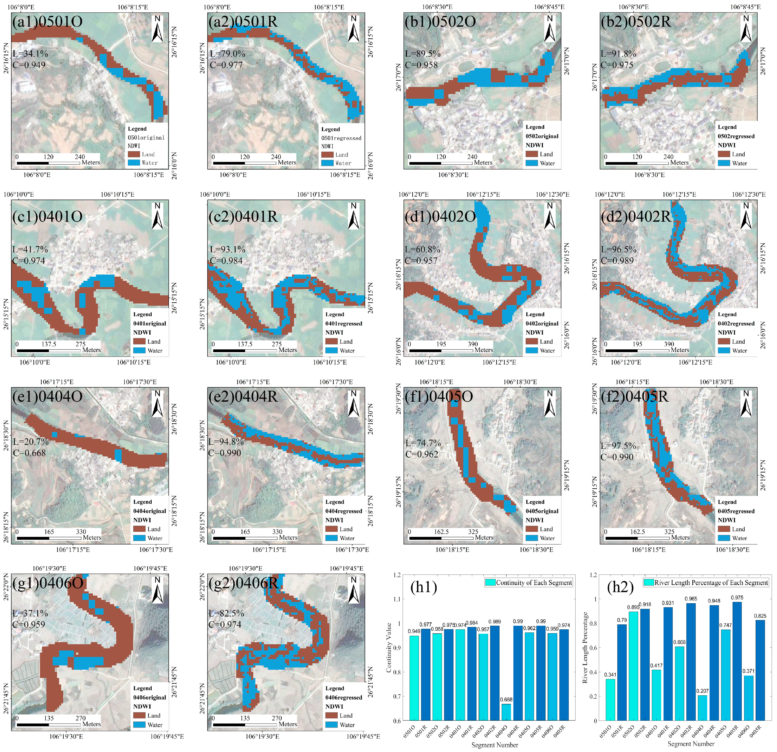
For each of the seven segments, we applied identification of water bodies and riverbanks on the LS8 original images and LS8 regression images. The results showed that there were significant differences between the two images: in the original images, water bodies were discontinuous, the distribution of river width was uneven, and there were fewer pixels in the channels. In regressed images, the water bodies were more continuous, river width was evenly distributed, and the number of water pixels increased significantly, as shown in Figure 2.
Among the seven segments, the water bodies identified by LS8 original images were discontinuous, with an average water body continuity index of 0.918, while the index of regression images reached 0.983, an increase of 7.1%. Affected by the spectral characteristics of the water body, NDWI images from optical satellites, such as LS8, recognize regions with deep water depth, slow flow, and smooth water surface as water bodies, as shown in Figure 2(b1,c1,d1,g1). In these areas, the river channels are wide and there are bends in the river. Deep pools are can easily be found. In addition, the reaches with artificial dams in the river and high obstruction of water bodies have higher NDWI values, which are easy to identify [45]. Many of the areas identified as land in the river channels have shallow water depths and fast flow velocities. The NDWI value of the region with an unstable water surface is lower, so the water pixels of these reaches show poor water continuity and uneven river width distribution.
In Figure 2(a1,e1,f1), rivers are narrow or straight, and the water depth is not deep. Therefore, the water bodies identified from LS8 original images are mainly distributed in the center of the river, where the water pixels show uneven river width distribution and low continuity. In addition, the resolution of the LS8 original image is coarser than that of ST2, at approximately 30 m. The pixels close to the riverbank are usually in a mixed state of land and water, and it is difficult to separate them under the resolution of the original LS8 image. As seen from Figure 2(h1,h2), the average river length percentage in the regressed images increased from 51.2% to 90.7% after the method was applied, an increase of 40%. The LS8 image resolution reached 10 m after method application, with the help of ST2 images in the same period to determine the location of the water in the river. The NDWI value of areas with shallow depths or unstable surfaces also reached the level of other water bodies. The scope of identified water expanded, with water pixels distributed more evenly in the river. In addition, the pixels that originally mixed land and water were divided into water pixels with high NDWI values and land pixels with low NDWI values. The remaining water bodies were connected to the originally recognized water pixels, which improved continuity and solved the problem of water bodies with uneven distributions of river width being less recognizable due to the resolution effects.

3.2. Effect of Extension to Runoff Series from Multisource Data

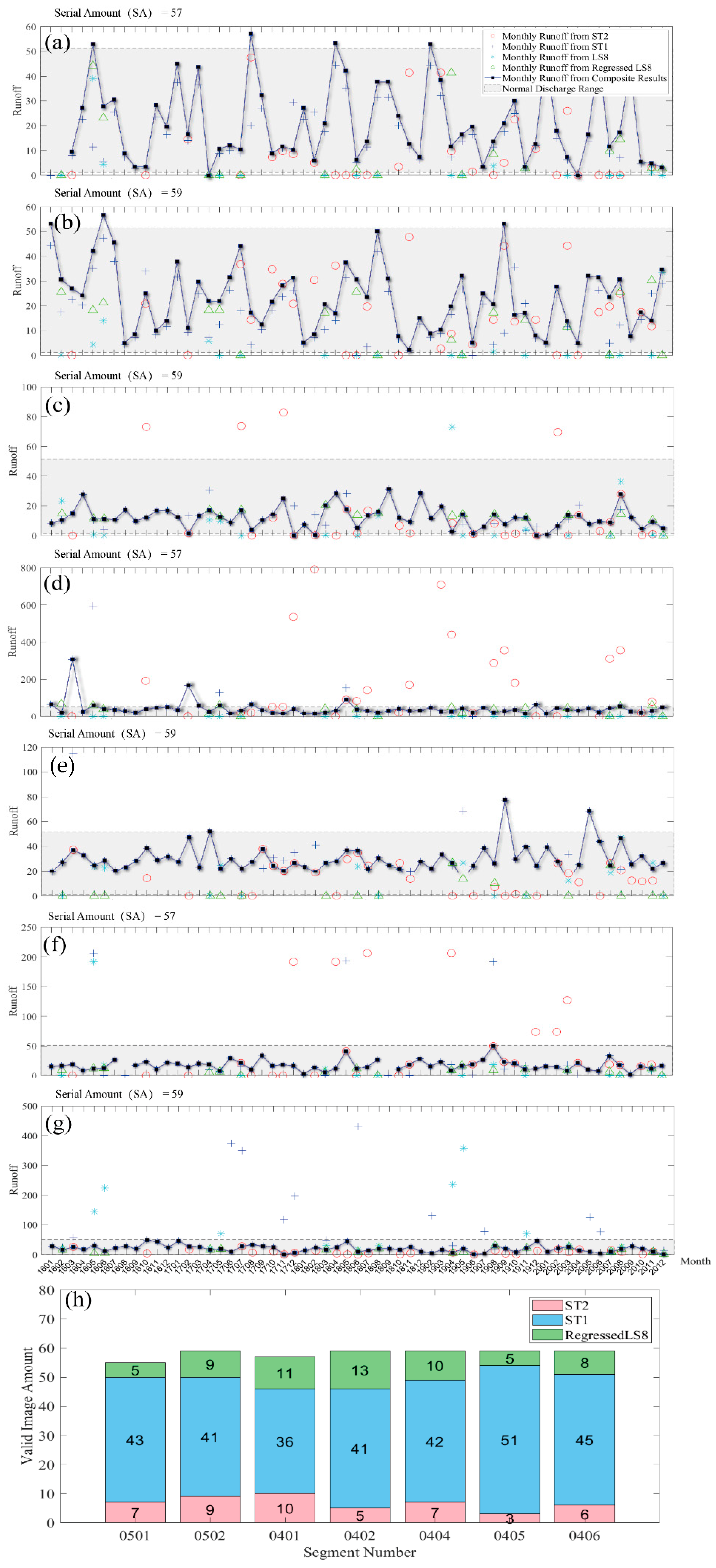
We constructed the river flow sequence of ST2 optical images, ST1 radar images, LS8 original optical images and LS8 regressed images and integrated the flow data into a composited flow sequence according to the in situ value series of typical years. The monthly flow data series of seven sections from 2016 to 2020 were obtained, as shown in Figure 3. As indicated in Figure 3a–g, only approximately 10 flow values were estimated in the sequences taken from the original optical images (LS8), while there were more than 50 comprehensive sequence values in the composited sequence, five times the original data. Compared with the results of various data sources, the composited sequence greatly extended the timespan of optical images and ensured the temporal continuity of flow.
As seen from the figure, ST2 optical images and LS8 original optical images, the traditional data sources used by flow calculation, are affected by a large amount of cloud and fog in the research area. For 60 months over five years, the available data amount from seven sites was very small, with fewer than 30 data points from ST2 images and fewer than 20 data points from LS8 original images. In addition, due to thin cloud occlusion, the NDWI values of most pixels were generally higher when synthesizing optical images. This led to the overestimation of water body recognition when the recognition algorithm was learning to recognize water body or land pixels and mistakenly identified many areas covered by clouds as water bodies or land. As a result, the calculated flow reached improper extreme values within 0.1 m3/s or more than 100 m3/s.
As an active remote sensing data source, ST1 radar images are not affected by weather conditions, so without special interference, ST1 images can cover the timespan of the whole year and can be used as a complete flow calculation data source. However, radar satellites are different from optical satellites, as their imaging principle is to send electromagnetic pulses and receive echoes in the sensor, calculating underlying surface roughness based on the strength of the returned signal (backscatter). Backscatter from water features is similar to some other surface features, such as artificial ground, which reduces identification capability for water compared to optical images, especially in NDWI images. There is also often noise in water body recognition, as shown in the figure, where the non-flood season flow shows outliers greater than 20 m3/s.
The flow of LS8 regressed images after downscaling is within the flow range of typical years, which can be used as a reference value for correction of flow calculated from radar images in the non-flood season. The composited sequence retains the radar data long time span and excludes the improper extreme values in radar data with the aid of ST2 images with LS8 regressed images, as shown in Figure 3 in the sequence (a), (b), (c), (d). Reasonable optical image data are used as a supplement to the composited sequence to help reduce the emergence of improper extreme values in the flow data. If there are few improper extreme values in each data source, the composited sequence will filter and adjust the reasonable estimated flow results of each data source according to the annual distribution of typical years and synthesize the flow sequence that meets the annual distribution law of true values.

3.3. Accuracy Comparison between Runoff Results from Original and Regressed Images

After statistical regression downscaling of LS8 original images in a typical year (2016), it can be seen that the daily calculated flow results were closer to the measured true value, and the RMSE and MPE were greatly reduced, with a decrease in a range from 3 m3/s to 8 m3/s.
It is shown in Figure 2 that the continuity of water bodies improved after the method was applied. As seen from Figure 4 a,b, the daily flow accuracy of LS8 after regression downscaling was significantly improved. RMSE before regression was 13.5 m 3 / s , and after regression, it decreased to 5.4 m 3 / s , reducing by nearly 60%. This indicates that the discontinuity of the original images provided unreliable average river widths, which led to unstable discharges with an error of 13.5 m 3 / s on average, and this number decreased greatly with steadier average river widths provided by water bodies with better continuity. The MPE was reduced from approximately 216% to 44%, which shows that the average difference between the calculated discharge and observed discharge decreased from 10.9 m 3 / s to 4.22 m 3 / s . In the flood season, the RMSE of the two flow points decreased from 8.3 m 3 / s to 6.2 m 3 / s , with a reduction of 25%. The MPE decreased from 59% to 44%, indicating that the average difference between calculated discharge and observed discharge decreased from 6.73 m 3 / s to 3.27 m 3 / s . According to the distribution of flow points, flows estimated before regression come with obvious random errors, which are distributed on both sides of the 1:1 line and in general relatively far away from the 1:1 line. After downscaling, the estimated flow was distributed near the 1:1 line. The whole fitting line slope was close to 1, with a smaller random error, and the fitting line R 2 was 0.77. This shows that the fitting result of the flow point is reliable.
The accuracy of the composited monthly flow series also improved after regression. As shown in Figure 4c,d, the overall RMSE of monthly flow reached 11.7 m 3 / s before regression but decreased to 7.4 m 3 / s after regression, a decrease of nearly 37%. At the same time, MPE was reduced from 213% to 107%. This means the average difference between the calculated discharge and observed discharge decreased from 10.0 m 3 / s to 5.99 m 3 / s which is a significant effect. In the flood season, the RMSE of the three flows decreased from 9.43 m 3 / s to 5.71 m 3 / s . The MPE decreased from 46% to 29%, as the average difference between the calculated discharge and observed discharge in flood season decreased from 8.93 m 3 / s to 4.27 m 3 / s . In addition, from the distribution of flow points in the figure, the accuracy was significantly improved: the systematic error of the original monthly flow is obvious, and more flow points are distributed on the right of the 1:1 line, indicating that the estimated flow is too large. The fitting line R 2 is only 0.008, indicating that the data are relatively discrete. After regression, the systematic error was significantly reduced so that the flow points were closer to the 1:1 line, with the slope of the fitted line closer to 1, and R 2 reaching approximately 0.4, which indicates higher concentration and more reliable results.
It can be found from the figure that the accuracy of flow in the flood season is generally higher than that in the non-flood season, and the systematic error is smaller. In the non-flood season, the estimated flow is more likely to be larger, which is discussed in Section 4.3.

4. Discussion

4.1. What Affects the Accuracy of This Method?

As shown in Figure 3, under the influence of thin cloud and noise errors in the study area, the water clarity of the image is low and the flow estimation is far overestimated. When the water clarity and natural conditions in the images change, the water area distribution and flow accuracy estimated by the method show significant changes. In fact, water clarity indicates the difference between the reflection characteristics of water and land, which can be observed most directly from their NDWI value. As we have chosen different water and land area in the images, the difference between these thresholds varies. This study defines water clarity alone as the degree of distinction between the NDWI threshold of water pixels and land pixels in the remote sensing images, which is named P i to be the judgment standard.
P i = V w a t e r V l a n d
In the equation, P i is the water clarity of each segment, V w a t e r is the NDWI threshold value of water, and V l a n d is the NDWI threshold value of land.
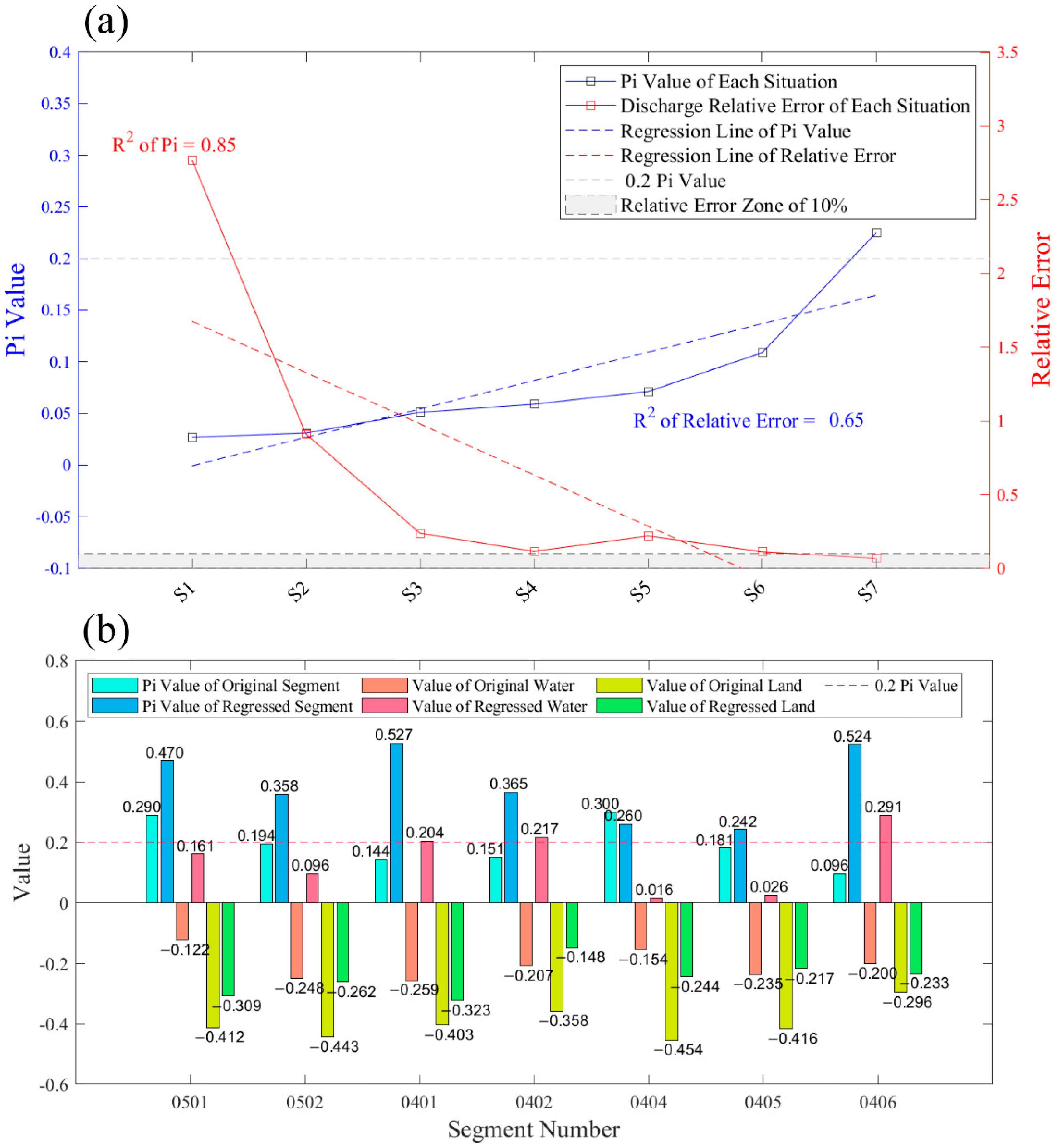
We analyzed section 0406 and set up seven situations in this section. In each situation, the NDWI thresholds of water bodies and land surfaces were different due to different selections of water bodies and land surface areas. In Figure 5a, water clarity values are arranged by gradients from 0 to 0.25. As the water clarity value increases, the flow error is reduced. Its change tendency is not always the same, especially in situations where the water clarity value is less than 0.05 and the flow relative errors are 100% or more. In these situations, a slight increase in the water clarity value leads to a significant decrease in the flow rate error, which is due to the similarity of water and land NDWI values, resulting in a large water body identification error. As the images in the water become clearer and the water clarity value increases to over 0.05, the surfaces of the water and land differ more and the flow error starts to fall. When the water clarity value is over 0.2, the flow errors can reach 6% and the rate of decrease slows. This indicates that when water clarity exceeds 0.2, the difference between the water body identification error and the flow estimation accuracy is negligible, and the influence of the flow rate on estimating the effect is improved.
As seen from Figure 5b, in the original sections where the regression method was not applied, most of the water clarity values are below 0.2, with only two sections exceeding 0.2. At present, the downscaling method we adopt can significantly raise the water clarity values up to above 0.2 in the corresponding sections, but there are still some sections whose water clarity values show little effect from the regression method, due to environmental conditions or cloud cover. According to the relationships in Figure 5, the applied method in this paper helps raise water clarity values up to above 0.2, and the flow errors in the corresponding sections can thereby show a substantial decline. Further application in the future and improvement of this method should focus more on adjusting and controlling water clarity values in the range above 0.2, verifying the effect of water clarity values on the reduction of flow errors.

4.2. What Are the Main Influences on the Long-Term Discharge Generation of Small- and Medium-Scale Rivers?

The main factors affecting the production of long-term series flow data for small- and medium-scale rivers in this region are meteorological conditions such as clouds and fog, geographical characteristics such as river width distribution, noise errors of optical and radar satellite sensors, and the availability of remote sensing image data.
When remote sensing images are taken to directly estimate small- and medium-scale river flows at middle and low latitudes, the most influential factor is that these areas are seriously affected by clouds, shadows, and fog. Even relatively thin clouds and fog, due to their various types and different spectral attributes, cause different changes in remote sensing image values, such as NDWI [18,46]. The value of cloud shadow is close to that of ground objects such as water bodies, which leads to the error of misidentifying water bodies even in images without direct occlusion by clouds. [19]. Most ST2 and LS8 optical images in the study area are shielded by clouds, making it difficult to see the distribution of river channels and water bodies. This also leads to the fact that even though LS8 and ST2 satellites have a short revisit cycle, with averages of 25 and 47 images per year, respectively, only four and nine of these image sets could clearly identify river channels each year, which made it difficult to meet the requirements for long sequence inversion.
Small- and medium-scale rivers are more difficult to accurately identify due to their narrow channels and small water surface area, which were not easy to obtain from images due to resolution limitation and interference from other ground objects. As can be seen from Figure 2, many pixels near the river banks were recognized as land before our method was applied. This is because that most of these pixels were mixed pixels with both water and land. Under Landsat-8’s spatial resolution of 30 m, these pixels could cover half of the river area and caused large errors. Under high resolution of 10 m with our method applied, more pixels were divided and many of them were classified as water. Meanwhile, there were still some pixels with mixed water and land, which is inevitable. Compared with the original results, more water area has already been correctly identified.
Moreover, even with the improvement in spatial resolution, a large number of artificial structures, such as paddy fields and roads around river channels, are also mistakenly identified as water areas, which causes more interference with river channel recognition [44,45,47], resulting in extreme outliers in water body recognition in the images and discontinuous estimation of river flow. In the period not covered by clouds and fog, the river in the image is only shown as one pixel wide in the LS8 images. In areas with a high degree of vegetation coverage on the bank or where a bridge spans the river, the edge of the water body cannot be identified accurately, so the direction and width of the flow cannot be extracted from the remote sensing images. In the ST2 image, the water body performance is better, and the water area identification and flow estimation results of the river center are improved due to the higher resolution, but there are also problems due to vegetation and artificial structures.
In addition, noise errors caused by the imaging principles of different sensors also affect the production of long series flow data in small- and medium-scale rivers. Taking ST2 and ST1 as examples, they represent passive optical remote sensing sensors and active radar remote sensing sensors, respectively. As mentioned above, the noise of optical images mainly comes from clouds and fog, while the noise of radar SAR images mainly comes from the shadows of mountains and buildings, flat road surfaces and ships in water [28,34,44]. A smooth road surface around the river or the shadow of a mountain may make the identification of the water area too large or too small, which does not meet the conditions of river calculation and has a certain impact on the calculation of long series flow.
It should be noted that at present, most spatial resolutions of free remote sensing data are too coarse for small- and medium-scale rivers, and satellite sensors such as MODIS are completely unable to be used at resolutions below 250 m. The finest Sentinel series only started in 2016 and access to the more sophisticated GF-2 commercial satellite is expensive and it has not seen widespread use. Therefore, LS8 is still mainly used for long sequence flow production.

4.3. What Are the Differences between Discharges in Flood and Nonflood Seasons?

In part 3.3, we carry out the accuracy verification of the daily and monthly flow sequences of section 0406 in 2016, as shown in Figure 4. We find that the flow estimation accuracy was higher in the flood season than in the non-flood season. This is because the actual channel shape distribution was more complex. As we adopted the method of hydraulic geometric fitting of the river, there were some errors in the fitted shape of the channel under the water surface. The underwater part may be controlled by different hydraulic geometry relations corresponding to the wet season and dry season. Here, we calculated the river width error and flow error according to the true and estimated flow values of section 0406 in 2016 and their corresponding river widths, which were grouped according to the flood season and non-flood season and ranked according to the river width error from small to large. Figure 6 shows that the flow rate error growth rate was far lower than that of the river width error in the flood season, while the error flow growth rate during most of the non-flood season was higher than that of river width, which indicates that error caused by river width recognition had a larger impact on flow accuracy in the non-flood season than in the flood season. Our algorithm is more sensitive to large flow calculations; relatively speaking, the flow calculation error of low discharge may be larger. This is because when the flow is low in the non-flood season, the water was mainly distributed in the middle of the channel, and the shape of the center of the channel was deep and narrow with a V-shape rather than wide and shallow with a U-shape. With the slight change in the river width in this period, hydraulic aspects of the change in the flow were relatively more significant. In the flood season, the change in discharge with river width was not significant. The influence of complex river shape on the relationship between river width and discharge exists not only with in a single section but also with a certain deviation between upper and lower sections of the same reach. The hydraulic geometric relationship of stations may also change with changes in time, climate and topographic conditions. If the river shape and hydraulic geometry are fitted according to the average width of the flood and non-flood seasons, and different hydraulic formulas are used to calculate them, the complex morphological changes of the river channel can be taken into account, and the errors associated with the flood and non-flood seasons can be reduced.

5. Conclusions

To solve the problems associated with long-term small- and medium-scale river flow monitoring, we developed a new method based on statistical linear regression and Remote Sensing Hydrologic Stations to achieve long sequence flow from high-precision remote sensing images. With remote sensing images downscaled from 30 m to 10 m resolution and multisource data integration of optical satellites, radar satellites and UAVs, river flow can be calculated with high accuracy and composited according to the rationality of flow data. In this case, different information can be obtained from multi-source remote sensing images, which indeed raises the utilization efficiency of these data sources. The method was tested on the Yunnan-Guizhou Plateau in southwest China and the accuracy of the results was verified. The results showed that (1) after this method was applied, the spatial resolution of Landsat-8 was significantly improved by linear downscaling and the water continuity index was increased by 7.1%. The average river length percentage in the channel reached 90.7%, an increase of 40%; (2) with the help of multisource data, the outliers of the flow series were greatly reduced, and the timespan was increased from approximately 10 data points in 5 years to more than 54 monthly flow data points, ensuring the temporal continuity of the calculated flow; (3) after downscaling, the images with better water continuity showed more stable river width, which reduced the RMSE of the Landsat-8 estimated flow from 13.5 m 3 / s to 5.4 m 3 / s , only 2/5 of the original. The MPE was reduced from 216% to 44%, specifically from 10.9 m 3 / s to 4.22 m 3 / s . The RMSE and MPE of the synthetic monthly sequence were also reduced, from 11.7 m 3 / s to 7.4 m 3 / s and from 10.0 m 3 / s to 5.99 m 3 / s respectively, after this method was applied. Our method is a complete set of mechanisms for image acquisition, downscaling, flow estimation and composited adjustment. It can be applied universally for flow estimation of small- and medium-scale rivers. Our method can provide a means of flow estimation for areas where the scope of remote sensing methods has previously been limited. In addition, this method can directly obtain continuous and high-precision water area inundation maps without the interference of weather and time, which will be of great value for water resource management and utilization.

Author Contributions

Conceptualization, H.L. and Y.Z.; methodology, S.Y. and H.L.; software, S.Y. and Z.P.; validation, Y.Z.; investigation, Y.Z., Z.P. and Y.L.; resources, Y.L. and X.W.; writing—original draft preparation, H.L. and Y.Z.; writing—review and editing, H.L. and Y.Z.; visualization, Y.Z.; supervision, H.L. and S.Y.; project administration, S.Y. All authors have read and agreed to the published version of the manuscript.

Funding

This research was funded by the National Natural Science Foundation of China (Grant Nos. U1812401, 41801334), Key Project of Philosophy and Social Sciences Planning in Guizhou Province (19GZZD07), the Open Research Fund Program of State Key Laboratory of Hydroscience and Engineering (sklhse-2021-A-04), the Opening Fund of State Key Laboratory of Geohazard Prevention and Geoenvironment Protection (Chengdu University of Technology, SKLGP2020K005), and the Fundamental Research Funds for the Central Universities (2017NT11).

Data Availability Statement

Not applicable.

Conflicts of Interest

The authors declare no conflict of interest.

References

  1. Alsdorf, D.E.; Rodríguez, E.; Lettenmaier, D.P. Measuring surface water from space. Rev. Geophys. 2007, 45. [Google Scholar] [CrossRef]
  2. Ashmore, P.; Sauks, E. Prediction of discharge from water surface width in a braided river with implications for at-a-station hydraulic geometry. Water Resour. Res. 2006, 42. [Google Scholar] [CrossRef]
  3. Bao, W.; Zhang, X.; Yu, Z.; Qu, S. Real-Time Equivalent Conversion Correction on River Stage Forecasting with Manning’s Formula. J. Hydrol. Eng. 2011, 16, 1–9. [Google Scholar] [CrossRef] [Green Version]
  4. Birkett, C.M.; Mertes, L.A.K.; Dunne, T.; Costa, M.H.; Jasinski, M.J. Surface water dynamics in the Amazon Basin: Application of satellite radar altimetry. J. Geophys. Res. Atmos. 2002, 107, LBA 26-1–LBA 26-21. [Google Scholar] [CrossRef]
  5. Bjerklie, D.M.; Dingman, S.L.; Vorosmarty, C.J.; Bolster, C.H.; Congalton, R.G. Evaluating the potential for measuring river discharge from space. J. Hydrol. 2003, 278, 17–38. [Google Scholar] [CrossRef]
  6. Bjerklie, D.M.; Moller, D.; Smith, L.C.; Dingman, S.L. Estimating discharge in rivers using remotely sensed hydraulic information. J. Hydrol. 2005, 309, 191–209. [Google Scholar] [CrossRef]
  7. Chang, X.Y. Studies on Guizhou Less Sunny More Rainy Days. Master’s Thesis, Guizhou Normal University, Guiyang, China, 2014. [Google Scholar]
  8. Chastain, R.; Housman, I.; Goldstein, J.; Finco, M.; Tenneson, K. Empirical cross sensor comparison of Sentinel-2A and 2B MSI, Landsat-8 OLI, and Landsat-7 ETM+ top of atmosphere spectral characteristics over the conterminous United States. Remote Sens. Environ. 2018, 221, 274–285. [Google Scholar] [CrossRef]
  9. Chen, J.; Yu, J.; Bai, X.; Zeng, Y.; Wang, J. Fragility of karst ecosystem and environment: Long-term evidence from lake sediments. Agric. Ecosyst. Environ. 2020, 294, 106862. [Google Scholar] [CrossRef]
  10. Chokmani, K.; Ouarda, T.B.M.J. Physiographical space-based kriging for regional flood frequency estimation at ungauged sites. Water Resour. Res. 2004, 40. [Google Scholar] [CrossRef]
  11. Dinar, S. The Geographical Dimensions of Hydro-politics: International Freshwater in the Middle East, North Africa, and Central Asia. Eurasian Geogr. Econ. 2012, 53, 115–142. [Google Scholar] [CrossRef]
  12. Duan, P.; Wang, M.; Lei, Y.; Li, J. Research on Estimating Water Storage of Small Lake Based on Unmanned Aerial Vehicle 3D Model. Water Resour. 2021, 48, 690–700. [Google Scholar] [CrossRef]
  13. Durand, M.; Rodriguez, E.; Alsdorf, D.E.; Trigg, M. Estimating River Depth From Remote Sensing Swath Interferometry Measurements of River Height, Slope, and Width. IEEE J. Sel. Top. Appl. Earth Obs. Remote Sens. 2009, 3, 20–31. [Google Scholar] [CrossRef]
  14. Flener, C.; Vaaja, M.; Jaakkola, A.; Krooks, A.; Kaartinen, H.; Kukko, A.; Kasvi, E.; Hyyppä, H.; Hyyppä, J.; Alho, P. Seamless Mapping of River Channels at High Resolution Using Mobile LiDAR and UAV-Photography. Remote Sens. 2013, 5, 6382–6407. [Google Scholar] [CrossRef] [Green Version]
  15. Huang, C.; Thomas, N.; Goward, S.N.; Masek, J.G.; Zhu, Z.; Townshend, J.R.G.; Vogelmann, J. Automated masking of cloud and cloud shadow for forest change analysis using Landsat images. Int. J. Remote Sens. 2010, 31, 5449–5464. [Google Scholar] [CrossRef]
  16. Immerzeel, W.; Droogers, P. Calibration of a distributed hydrological model based on satellite evapotranspiration. J. Hydrol. 2008, 349, 411–424. [Google Scholar] [CrossRef]
  17. Irish, R.R.; Barker, J.L.; Goward, S.N.; Arvidson, T. Characterization of the Landsat-7 ETM+ Automated Cloud-Cover Assessment (ACCA) Algorithm. Photogramm. Eng. Remote Sens. 2006, 72, 1179–1188. [Google Scholar] [CrossRef]
  18. Jiang, H.; Wang, M.; Hu, H.; Xu, J. Evaluating the Performance of Sentinel-1A and Sentinel-2 in Small Waterbody Mapping over Urban and Mountainous Regions. Water 2021, 13, 945. [Google Scholar] [CrossRef]
  19. Borah, D.K.; Bera, M. Watershed-scale hydrologic and nonpoint-source pollution models: Review of applications. Am. Soc. Agric. Eng. 2004, 47, 789–803. [Google Scholar] [CrossRef] [Green Version]
  20. Kebede, M.G.; Wang, L.; Yang, K.; Chen, D.; Li, X.; Zeng, T.; Hu, Z. Discharge Estimates for Ungauged Rivers Flowing over Complex High-Mountainous Regions based Solely on Remote Sensing-Derived Datasets. Remote Sens. 2020, 12, 1064. [Google Scholar] [CrossRef] [Green Version]
  21. Kim, Y.; Park, N.-W. Comparison of regression models for spatial downscaling of coarse scale satellite-based precipitation products. In Proceedings of the 2017 IEEE International Geoscience and Remote Sensing Symposium (IGARSS), Fort Worth, TX, USA, 23–28 July 2017; pp. 4634–4637. [Google Scholar] [CrossRef]
  22. Lin, C.-H.; Tsai, P.-H.; Lai, K.-H.; Chen, J.-Y. Cloud Removal from Multitemporal Satellite Images Using Information Cloning. IEEE Trans. Geosci. Remote Sens. 2012, 51, 232–241. [Google Scholar] [CrossRef]
  23. Liu, Y.; Gupta, H.V. Uncertainty in hydrologic modeling: Toward an integrated data assimilation framework. Water Resour. Res. 2007, 43. [Google Scholar] [CrossRef]
  24. Liu, Y.; Zhang, W.; Zhang, Z. A conceptual data model coupling with physically-based distributed hydrological models based on catchment discretization schemas. J. Hydrol. 2015, 530, 206–215. [Google Scholar] [CrossRef]
  25. Lou, H.; Wang, P.; Yang, S.; Hao, F.; Ren, X.; Wang, Y.; Shi, L.; Wang, J.; Gong, T. Combining and Comparing an Unmanned Aerial Vehicle and Multiple Remote Sensing Satellites to Calculate Long-Term River Discharge in an Ungauged Water Source Region on the Tibetan Plateau. Remote Sens. 2020, 12, 2155. [Google Scholar] [CrossRef]
  26. Lumbroso, D.; Gaume, E. Reducing the uncertainty in indirect estimates of extreme flash flood discharges. J. Hydrol. 2012, 414–415, 16–30. [Google Scholar] [CrossRef] [Green Version]
  27. McFeeters, S.K. The use of the Normalized Difference Water Index (NDWI) in the delineation of open water features. Int. J. Remote Sens. 1996, 17, 1425–1432. [Google Scholar] [CrossRef]
  28. Milly, P.C.D.; Dunne, K.A.; Vecchia, A.V. Global pattern of trends in streamflow and water availability in a changing climate. Nature 2005, 438, 347–350. [Google Scholar] [CrossRef]
  29. Morel, M.; Booker, D.J.; Gob, F.; Lamouroux, N. Consistent Theoretical and Empirical Predictions of at-a-Station Hydraulic Geometry Exponents in Stream Reaches. Water Resour. Res. 2020, 56, e2020WR027242. [Google Scholar] [CrossRef]
  30. Passalacqua, P.; Trung, T.D.; Foufoula-Georgiou, E.; Sapiro, G.; Dietrich, W.E. A geometric framework for channel network extraction from lidar: Nonlinear diffusion and geodesic paths. J. Geophys. Res. Earth Surf. 2010, 115, F01002. [Google Scholar] [CrossRef] [Green Version]
  31. Platnick, S.; King, M.D.; Ackerman, S.A.; Menzel, W.P.; Baum, B.A.; Riédi, J.C.; Frey, R.A. The MODIS cloud products: Algorithms and examples from terra. IEEE Trans. Geosci. Remote Sens. 2003, 41, 459–473. [Google Scholar] [CrossRef] [Green Version]
  32. Rusnák, M.; Sládek, J.; Kidová, A.; Lehotský, M. Template for high-resolution river landscape mapping using UAV technology. Measurement 2018, 115, 139–151. [Google Scholar] [CrossRef]
  33. Spiliotopoulos, M.; Adaktylou, N.; Loukas, A.; Michalopoulou, H.; Mylopoulos, N.; Toulios, L. A spatial downscaling pro-cedure of MODIS derived actual evapotranspiration using Landsat images at central Greece. In Proceedings of the First International Conference on Remote Sensing and Geoinformation of the Environment (RSCy2013), Paphos, Cyprus, 5 August 2013. [Google Scholar] [CrossRef]
  34. Vörösmarty, C.J.; McIntyre, P.B.; Gessner, M.O.; Dudgeon, D.; Prusevich, A.; Green, P.; Glidden, S.; Bunn, S.E.; Sullivan, C.A.; Liermann, C.R.; et al. Global threats to human water security and river biodiversity. Nature 2010, 467, 555–561. [Google Scholar] [CrossRef] [PubMed]
  35. Wang, Z.; Liu, J.; Li, J.; Meng, Y.; Pokhrel, Y.; Zhang, H. Basin-scale high-resolution extraction of drainage networks using 10-m Sentinel-2 imagery. Remote Sens. Environ. 2021, 255, 112281. [Google Scholar] [CrossRef]
  36. Wu, G.; Liu, Y. Downscaling Surface Water Inundation from Coarse Data to Fine-Scale Resolution: Methodology and Accuracy Assessment. Remote Sens. 2015, 7, 15989–16003. [Google Scholar] [CrossRef] [Green Version]
  37. Xu, K.; Zhang, J.; Watanabe, M.; Sun, C. Estimating river discharge from very high-resolution satellite data: A case study in the Yangtze River, China. Hydrol. Process. 2004, 18, 1927–1939. [Google Scholar] [CrossRef]
  38. Yamazaki, D.; Ikeshima, D.; Sosa, J.; Bates, P.D.; Allen, G.H.; Pavelsky, T.M. MERIT Hydro: A High-Resolution Global Hydrography Map Based on Latest Topography Dataset. Water Resour. Res. 2019, 55, 5053–5073. [Google Scholar] [CrossRef] [Green Version]
  39. Yang, S.; Bai, J.; Zhao, C.; Lou, H.; Zhang, C.; Guan, Y.; Zhang, Y.; Wang, Z.; Yu, X. The assessment of the changes of biomass and riparian buffer width in the terminal reservoir under the impact of the South-to-North Water Diversion Project in China. Ecol. Indic. 2018, 85, 932–943. [Google Scholar] [CrossRef]
  40. Yang, S.; Guan, Y.; Zhao, C.; Zhang, C.; Bai, J.; Chen, K. Determining the influence of catchment area on intensity of gully erosion using high-resolution aerial imagery: A 40-year case study from the Loess Plateau, northern China. Geoderma 2019, 347, 90–102. [Google Scholar] [CrossRef]
  41. Yang, S.; Li, C.; Lou, H.; Wang, P.; Wang, J.; Ren, X. Performance of an Unmanned Aerial Vehicle (UAV) in Calculating the Flood Peak Discharge of Ephemeral Rivers Combined with the Incipient Motion of Moving Stones in Arid Ungauged Regions. Remote Sens. 2020, 12, 1610. [Google Scholar] [CrossRef]
  42. Yang, S.; Wang, J.; Wang, P.; Gong, T.; Liu, H. Low Altitude Unmanned Aerial Vehicles (UAVs) and Satellite Remote Sensing Are Used to Calculated River Discharge Attenuation Coefficients of Ungauged Catchments in Arid Desert. Water 2019, 11, 2633. [Google Scholar] [CrossRef] [Green Version]
  43. Yang, S.; Wang, P.; Lou, H.; Wang, J.; Zhao, C.; Gong, T. Estimating River Discharges in Ungauged Catchments Using the Slope–Area Method and Unmanned Aerial Vehicle. Water 2019, 11, 2361. [Google Scholar] [CrossRef] [Green Version]
  44. Zhang, X.; Yan, X. A new statistical precipitation downscaling method with Bayesian model averaging: A case study in China. Clim. Dyn. 2015, 45, 2541–2555. [Google Scholar] [CrossRef]
  45. Zhou, N.; Li, X.; Shen, Z.; Wu, T.; Luo, J. Geo-Parcel-Based Change Detection Using Optical and SAR Images in Cloudy and Rainy Areas. IEEE J. Sel. Top. Appl. Earth Obs. Remote Sens. 2020, 14, 1326–1332. [Google Scholar] [CrossRef]
  46. Zhu, Z.; Wang, S.; Woodcock, C.E. Improvement and expansion of the Fmask algorithm: Cloud, cloud shadow, and snow detection for Landsats 4–7, 8, and Sentinel 2 images. Remote Sens. Environ. 2015, 159, 269–277. [Google Scholar] [CrossRef]
  47. Zhu, Z.; Woodcock, C.E. Object-based cloud and cloud shadow detection in Landsat imagery. Remote Sens. Environ. 2012, 118, 83–94. [Google Scholar] [CrossRef]
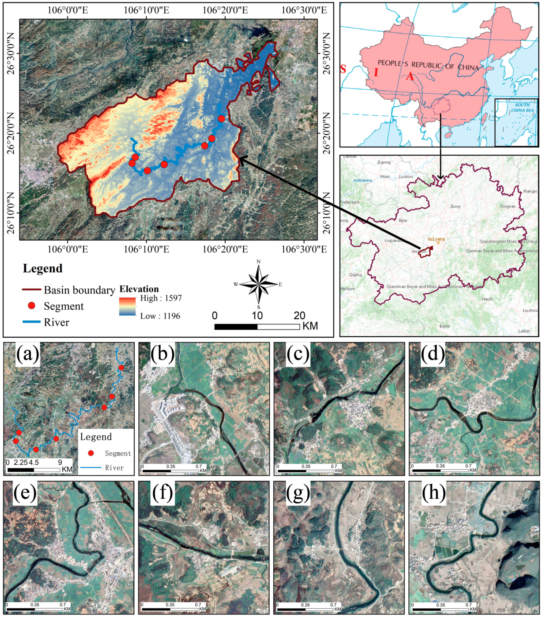
Figure 1. Overview of the research area, including (a) the distribution of Remote Sensing Hydrology Stations in the Xingjiang River basin; (bh) the river conditions and surrounding environment of each segment. Satellite images are collected from Google Earth.
Remotesensing 14 01798 g001
Figure 2. Water recognition distribution from original and regressed LS8 images. Figures (ag) represent the water body distribution in the map before and after the method was applied to segments 0501, 0502, 0401, 0402, 0404, 0405 and 0406. In each group, 1 represents the original image, 2 represents the regressed image. Group h represents the statistical variation of seven segments in two parameters: continuity (h1) and river length percentage (h2). Bars in light blue represent original images, bars in dark blue represent regressed images.
Remotesensing 14 01798 g002
Figure 3. Calculated flow sequences of each segment. In the figure, subfigure (ag) represent sections 0501, 0502, 0401, 0402, 0404, 0405 and 0406, respectively. In each sequence, red circles represent ST2 images, cyan meter characters stand for LS8 original images, blue crosses for ST1 radar images, and green triangles for LS8 regressed images. The dark square dotted line represents the composited flow sequence after adjustment. Subfigure (h) each column represents the number of composited flow values and the component source of the section. Green represents data from LS8 regressed images, blue from ST1 radar images, and red from ST2 optical images. The number of specific sources is marked in the corresponding color block.
Remotesensing 14 01798 g003
Figure 4. Correlation between estimated flow and measured flow. In the figure, (a,b) represent the comparison between the results of estimated flow and measured flow from LS8 images before and after regression, (c,d) represent the comparison results of composited monthly flow series and measured flow series before and after regression. For all plots, the black boxes are all calculated data points in all periods and the red boxes are calculated data points in the flood season.
Remotesensing 14 01798 g004
Figure 5. (a) Change diagram of flow relative errors and water clarity values, in which the red line represents the water clarity value and the blue line represents the relative error of the flow rate; (b) Statistical graph of the water clarity values of each section, in which the light blue column represents the original water clarity value of each section, the dark blue column represents the regressed water clarity value of each section, the orange column represents the original value of water in each section, the red column represents the regressed value of water in each section, the light green column represents the original value of land in each section, the dark green column represents the regressed value of land in each section, and the red dotted line represents the dividing line where the water clarity value is 0.2.
Remotesensing 14 01798 g005
Figure 6. Influence of river width error on flow error in (a) flood and (b) non-flood season. The solid blue line is flow error, the blue dotted line is its fitting line, the solid red line is river width error, and the dotted red line is its fitting line.
Remotesensing 14 01798 g006
Table 1. Datasets parameters.
Data TypeData NameSourceTimespan
(Time Resolution)
Spatial ResolutionPurpose
Remote sensing dataUAV remote sensingDJI Mavic Air 22020/11/4~2020/11/5 (/)5 cmConstruct digital river model
Landsat-8 surface reflectance (LS8)GEE2016~2020 (15 days)30 mIdentify water body
Sentinel-1 C-band synthetic aperture radar (ST1)GEE2016~2020 (10 days)10 m
Sentinel-2 surface reflectance (ST2)GEE2016~2020 (10 days)10 m
Measured dataMeasured velocity of flow and water depth of river sectionRotating Element Current Meter and Deeper Smart Sonar2020/11/4~2020/11/5 (/)/Establish RSHS
Statistical dataDaily measured dischargeHydrologic Yearbook2016 (day)/Obtain in-situ discharge data
Table 2. The parameter used in RSHS and their sources.
ParameterSymbolSource
River width-NDWI calculated from satellite images
Area of water passageARiver width and depth measured in situ with the mathematical relationship based on the shape of river channel
DischargeQManning formula
Conversion factorkRefer to [28,34,44]
RoughnessnIn situ measurement
Water-cycle lengthPRiver width and depth measured in situ with the mathematical relationship based on the shape of river channel
Hydraulic gradientSUAV images
Publisher’s Note: MDPI stays neutral with regard to jurisdictional claims in published maps and institutional affiliations.