Deep Feature Migration for Real-Time Mapping of Urban Street Shading Coverage Index Based on Street-Level Panorama Images

Abstract

Urban street shadows can provide essential information for many applications, such as the assessment and protection of ecology and environment, livability evaluation, etc. In this research, we propose an effective and rapid method to quantify the diurnal and spatial changes of urban street shadows, by taking Beijing city as an example. In the method, we explore a novel way of transferring street characteristics to semantically segment street-level panoramic images of Beijing by using DeepLabv3+. Based on the segmentation results, the shading situation is further estimated by projecting the path of the sun in a day onto the semantically segmented fisheye photos and applying our firstly defined shading coverage index formula. Experimental results show that in several randomly selected sampling regions in Beijing, our method can successfully detect more than 83% of the shading changes compared to the ground truth. The results of this method contribute to the study of urban livability and the evaluation of human life comfort. The quantitative evaluation method of the shading coverage index proposed in this research has certain promotion significance and can be applied to shading-related research in other cities.

1. Introduction

Shadows are dark areas formed due to the occlusion of light from a light source [1], and there are often shadows on city streets, which are mainly generated by roadside buildings, trees and other urban landscapes blocking sunlight. Urban street shadows are of great significance in ecological environment evaluation and protection, livability evaluation and human life comfort evaluation. Studying urban street shadows will provide important parameters for the above applications. For example, people engage in many social and leisure activities on the streets [2]. In summer, excess heat could affect pedestrians’ comfort and lead to great health risks [3,4]. Studies have found that extremely high temperatures can increase mortality and morbidity in cities around the world [3,5,6], and it can effectively alleviate the effects of high temperatures in the shadows [7,8]. An accurate understanding of street shading and its changes is of great significance for reducing the harm caused by extreme heat and extreme weather to humans. Furthermore, the street is also a necessary element for the urban space [9], and exploring the shadow situation of a street can better understand the characteristics of a city [10].

Street shadows affect cities in many aspects, such as street thermal environments [7,10], residents’ health [5], tourism [11,12], urban planning [2,13], architectural design [13], etc. In this regard, some researchers have also done some exploration. For instance, Sun et al. [7] explored the relationship between urban street shadows and thermal vulnerability and proposed a research framework for assessing urban thermal vulnerability. Several other studies have also confirmed the health effects of outdoor shade, that increasing urban shade can reduce the chance of prolonged exposure to heat and ultraviolet rays, thereby reducing the risk of skin cancer [14,15]; Chen and Ng [10] verified that increasing urban shaded areas and public spaces can lead to more outdoor exercise. The results showed that in tourist cities, foreign tourists are more sensitive to the thermal environment and more eager for shaded spaces in hot summer than residents [16]. From the perspective of student travel, it is proved that urban sidewalk shadows are positively correlated with students’ summer travel willingness [17]. Similarly, Rodríguez-Algeciras et al. [18] used the level of shading as one of the research variables to assess urban livability. The results showed that shaded public open spaces can enhance living comfort and livability in cities.

The methods of shadow detection have been well explored. In small scenes such as a single street, researchers have made direct experimental observations on shadowed areas [19], which can extract the area and variation of shadows in detail. Some researchers use professional cameras to take fisheye photographs and calculate the sky view factors to measure shadows [20]. The shading conditions obtained by the above two methods can only represent the conditions of a specific small area, and exploring the shading of a large area requires a large amount of manually collected data or fisheye photos [21]. In addition, the sky view factor can be used to calculate shading coverage conditions, but it cannot calculate the dynamic changes of shadows. Since the sun’s path in the sky changes from day to day, shading changes at the same time of day [22]. Numerous two-dimensional [10,23] or three-dimensional [24] models are developed to calculate urban-scale shadow conditions [25,26]. For example, researchers quantified the height/width (H/W) ratio of urban streets to evaluate shadows, and street canyons with a larger H/W ratio generally have higher shading levels [23,27]. However, these types of calculations usually simplify the structure of the street canyon by assuming some parameters and conditions, without taking into account the effects of trees. Moreover, satellite images are also used to quantify shading conditions. For instance, Moro et al. [28] integrated satellite imageries and geographic information system (GIS) simulation tools for the analysis of shading profiles. Nonetheless, the image data captured by satellites cannot clearly capture more details of the streets on the ground [29,30]. The use of light detection and ranging (LiDAR) technology can effectively describe the geometrical details of urban areas [21,31] to calculate the shading conditions, but the cost of LiDAR technology is relatively high, and it is not suitable for application in a large space [31].

With the rapid development of computer vision and sensor techniques, researchers began to use street-level imageries and deep learning-based methods to explore shadows. Some scholars have proposed a method to automatically calculate the sky view factor using street view images, which effectively avoids the labor cost of manual calculation [25]. Sky view factors obtained with street view images have been shown to have high accuracy [32,33], providing a solid basis for city-level shading. By overlaying the sun’s path at a given location at different times with the corresponding fisheye images, it is possible to simulate whether the light reaching the ground is blocked by objects, such as buildings [12,34,35]. Currently, the evaluation of solar duration [32,35] and solar radiation [34,35] can be achieved using a combination of deep learning and imagery. They did not pay attention to the fine-grained variation of shadows on the diurnal and spatial scales and lacked the precise time, location and temporal variation of shadows in a certain spatial range. To the best of our knowledge, shade coverage usually refers to objects in space that block sunlight (such as buildings or trees, etc.) [19,35], but there is no index that directly quantifies shade coverage. However, so far, studies using semantic segmentation for shading estimation require the manual shadow labeling of data and training of models to achieve a certain segmentation accuracy [31,32,34]. This method is time-consuming and expensive [36,37]. In this regard, we explore a way of transferring street characteristics to semantically segment street-level panoramic images by using DeepLabv3+ and quantify the diurnal and spatial changes of shading coverage in our research. Specifically, the contributions of our research are as follows:

(1) For the first time, we design an efficient shadow extraction method based on deep feature transfer, which can save the time overhead of semantic segmentation model retraining and achieve stable shadow extraction results.

(2) We innovatively define and calculate the shading coverage index to provide the foundation for the follow-up research.

(3) For the first time, we map the diurnal and spatial distribution of shading coverage in Beijing at the scales of kilometer grid and road sections, respectively.

2. Materials and Methods

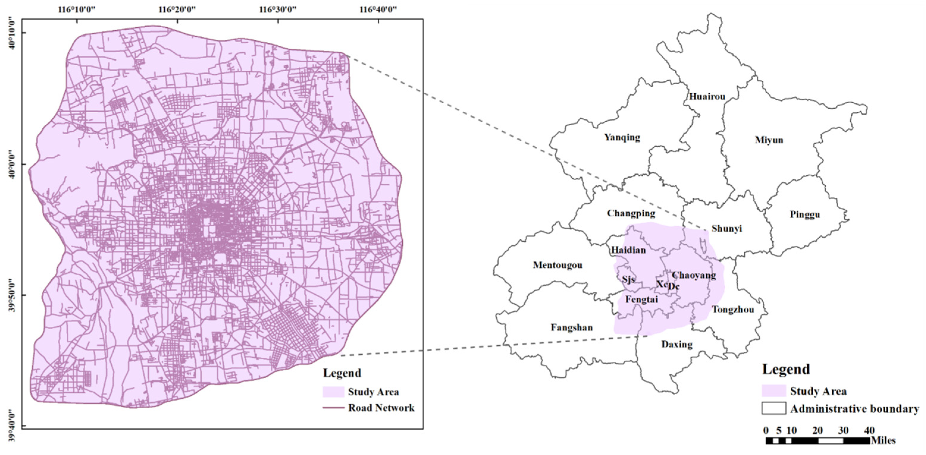
2.1. Study Area

Our study area is Beijing, China, with the north latitude range of 39°36′4.32″–41°02′26.91″ and the east longitude range of 115°47′55.78″–117°19′58.49″. Beijing has a warm temperate semi-humid continental monsoon climate, with high temperatures and the largest rain in summer [36]. As the capital of China, Beijing is the center of Chinese politics, economy, culture, education, technological innovation and international exchange. As of the end of November 2020, the permanent population of Beijing was about 21.893 million. We study the area within the sixth ring road of Beijing (Figure 1) which has a total area of 2267 km². This area includes most of the urban built-up area and a small part of the urban-rural fringe; 12 of the 16 administrative divisions in Beijing are partially or entirely located within the sixth ring road [37].

2.2. Data Source

Three main types of data sources were collected and used in this study. The road centerline within the sixth ring road in Beijing is extracted from AutoNavi’s road data. Baidu Street View (BSV) panoramas were obtained from the application program interface (API) of the Baidu Web Service. Administrative boundary vector data were provided by the Institute of Remote Sensing and Digital Earth, Chinese Academy of Sciences (http://www.aircas.cas.cn, 5 January 2021). The spatial data coordinate system adopts the unified geographic coordinate system GCS_WGS_1984.

2.3. Methods

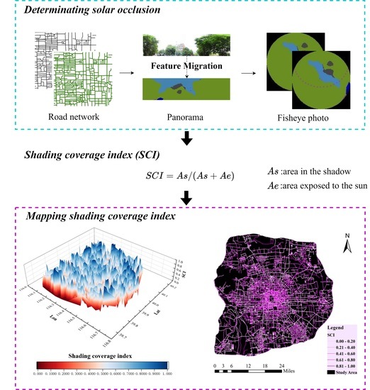
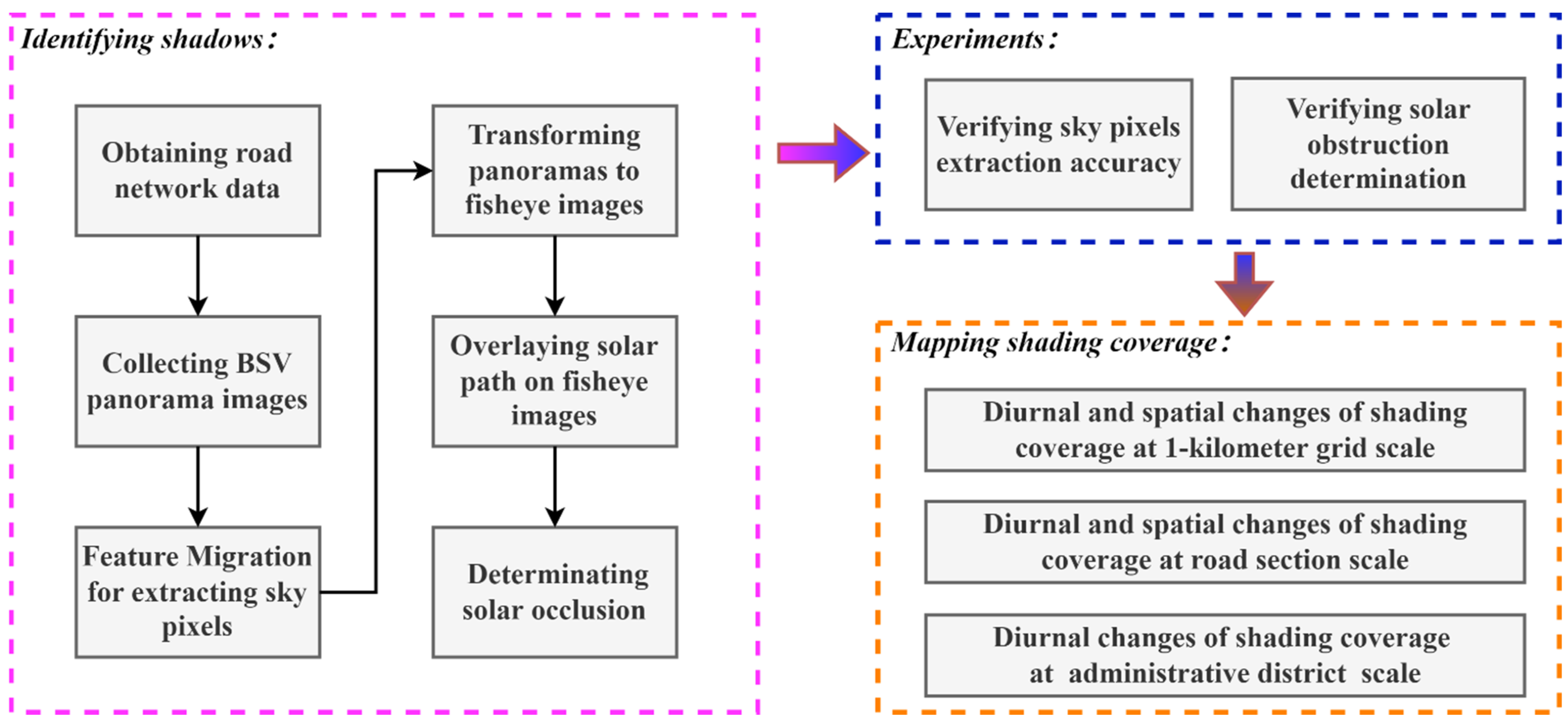
2.3.1. Research Framework

The framework of this research is shown in Figure 2, which is divided into three parts. Firstly, we obtain the road network data and BSV panoramas as data sources. On this basis, a series of processes are carried out, such as semantic segmentation based on deep feature migration, fisheye image conversion, and the projection of the sun path. This series of processes can determine whether a place is in shadow. Secondly, we conduct experiments to verify the accuracy of the sky pixels’ extraction and solar obstruction determination. Finally, according to our proposed formula, we calculate shading coverage in the study area and visualize its diurnal and spatial distribution by kilometer grid and the road section dimension.

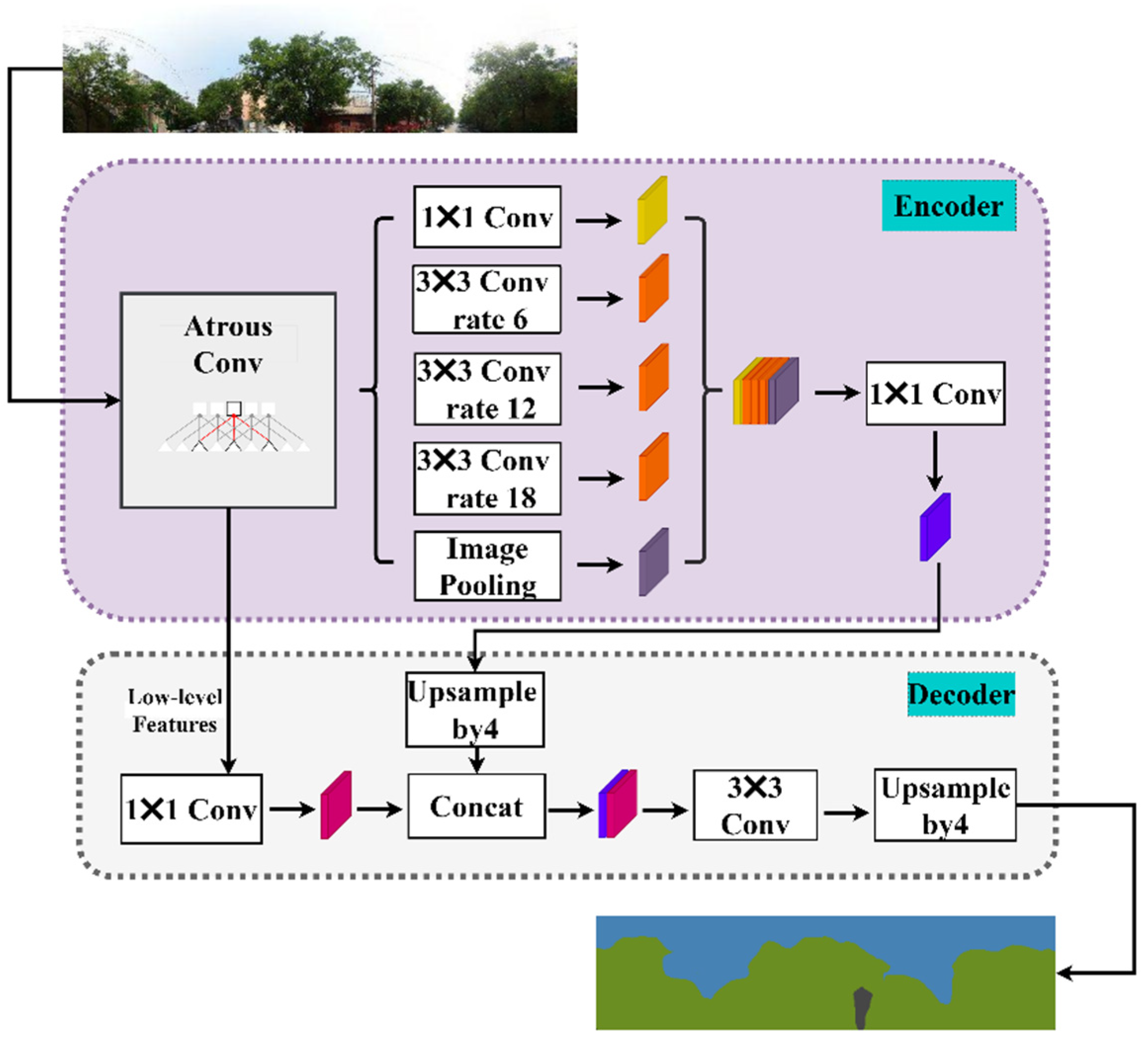
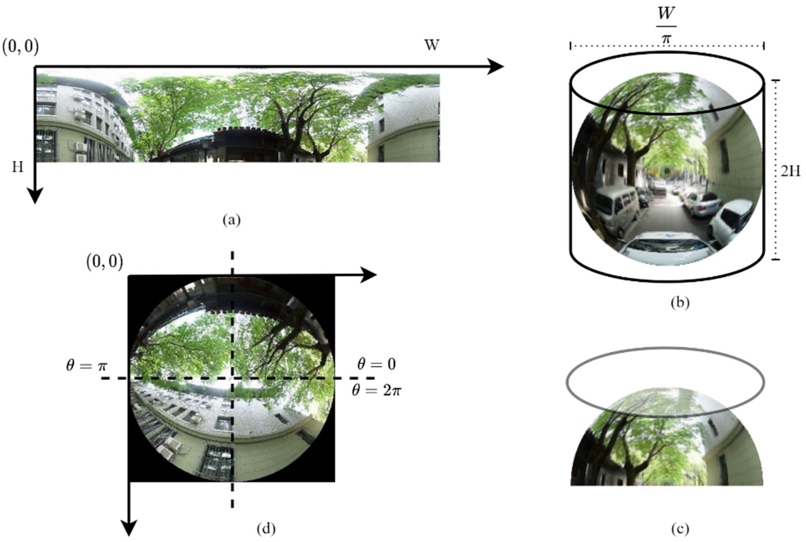
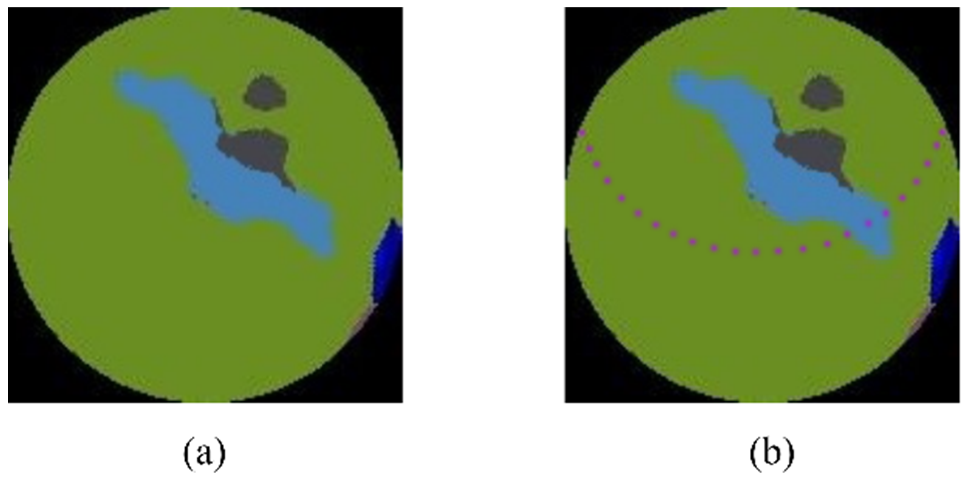
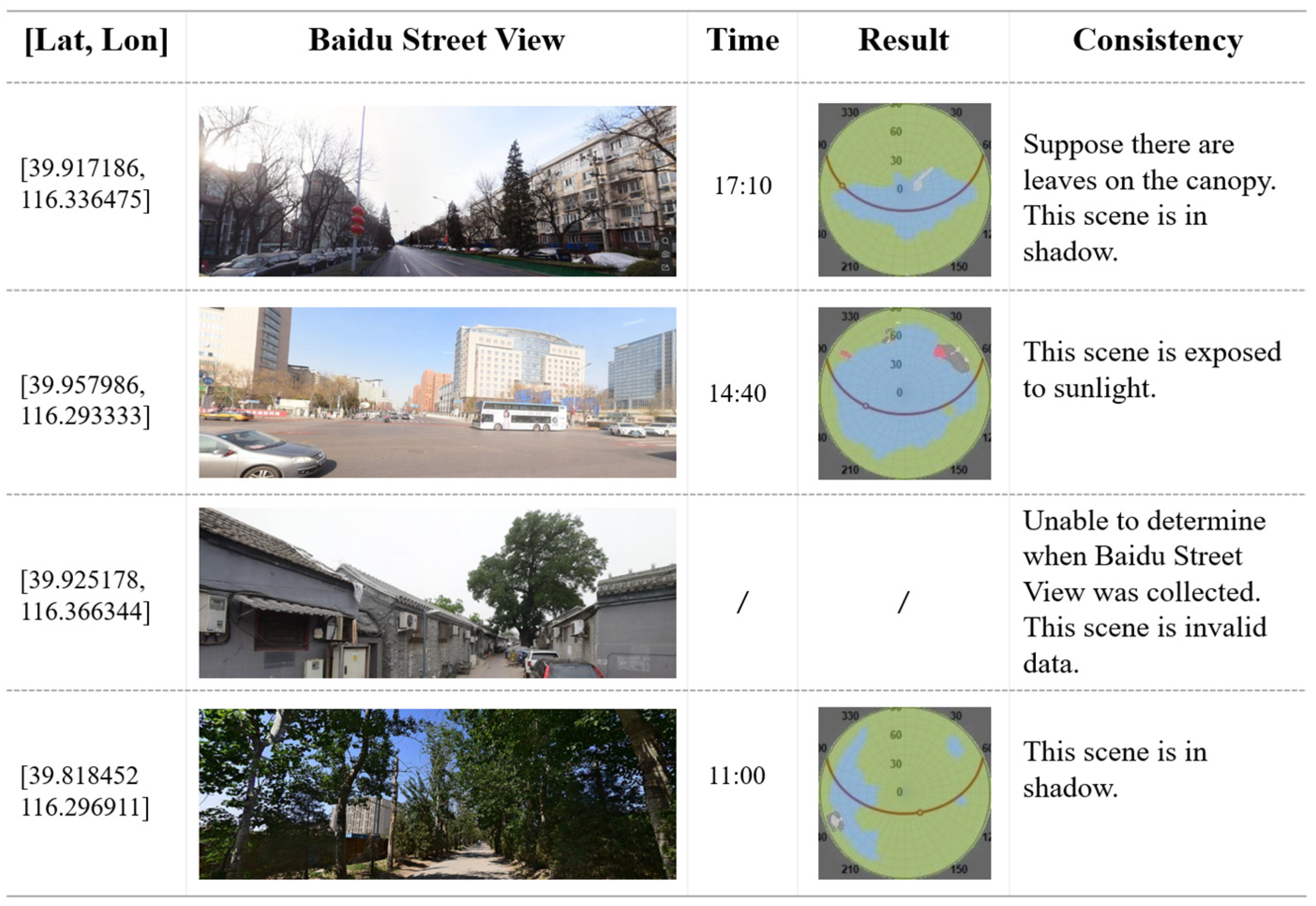
2.3.2. Identifying Shadows

Along with the road network in the study area, the street view sampling points were generated according to the distance interval of 50 m, and the latitude and longitude of all the sampling points were counted. We use the API of the Baidu map service to obtain panoramic images of sampling points. The Baidu panoramic street view image is generated from the eight original images captured by the cameras on a mobile vehicle [38].

The sky extraction is a necessary step in the shadow identification of street canyons using panoramas. We use the DeepLabv3+ model [39] trained on the Cityscapes dataset [40] to segment panoramic images to extract the sky, and Figure 3 displays the network structure based on DeepLabv3+. DeepLabv3+ combines the Spatial pyramid pooling (SPP) module and encode–decoder structure [39]. The SPP module is able to encode multi-scale contextual information while the latter module can capture sharper object boundaries by gradually recovering the spatial information [41]. Different from the previous semantic segmentation datasets, the Cityscape dataset is a street scene with a high diversity of land object categories. It includes about 50 different urban street scenes to increase the variety of street types, and images are collected over several months, with seasons spanning spring, summer and fall [40]. Due to the wide coverage of scene types in the cityscape dataset, the transferability and generality of the model for extracting deep features are improved.

Since shadows from objects of low height (e.g., below a person’s height) hardly affect human comfort, we crop each panorama image to preserve the portion above the street view vehicle’s horizontal viewing angle. This study needs to determine the positional relationship between the sun and the occluded pixels, and for convenience, we convert the panoramic image to a fisheye image. Essentially, a fisheye image is a representation of an azimuthal projection onto a plane tangent to the hemisphere [32]. As shown in Figure 4, projecting a panoramic image from a cylinder to an azimuthal coordinate system to generate a fisheye image is a common geometric transformation [42,43]. In geometric transformation, each pixel in the panoramic image uniquely corresponds to a pixel in the fisheye image. This research uses the method [35] to convert the image by assuming that $x \mathrm{and} y$ are the coordinates of the panoramic image. The $W$ and $H$ are the width and height of the cropped panorama, respectively. Then, the radius of the fisheye image is converted into $r_0=W/2\mathsf{\pi }$, the height and width of the fisheye image are both $W/\mathsf{\pi }$, then the coordinates corresponding to the center of the fisheye image are $\left(C_x ,C_{y }\right)$, which is calculated with Equation (1):

$$C_x=C_y=\frac{W}{2\mathsf{\pi }}.$$

(1)

The coordinate $\left(x_f ,y_f\right)$ and polar coordinate $\left(r, \theta \right)$ of each pixel in the fisheye image is related to the corresponding panoramic image coordinate $\left(x_p ,y_p\right)$ as follows, $x_p$,$\theta$ and $y_p$ are calculated by Equations (2)–(4), respectively:

$$x_p=\theta W/2\mathsf{\pi }$$

(2)

$$\theta =\{\begin{array}{c}\mathsf{\pi }/2+\arctan \left(y_f-C_y/x_f-C_x\right) x_f<C_x,\\ 3\mathsf{\pi }/2+\arctan \left(y_f-C_y/x_f-C_x\right) x_f>C_x,\end{array}$$

(3)

$$y_p=\frac{rH}{r_0},$$

(4)

where $r=\sqrt{{\left(x_f-C_x\right)}^2+{\left(y_f-C_y\right)}^2}$.

Since the center of the panorama is a true north direction in the real scene, the fisheye image obtained by the above geometric transformation is opposite to the direction of the sun path. In order to project the sun path later, we flip each fisheye image horizontally.

We convert the sun’s altitude and azimuth to a polar representation and project the sun’s path onto a fisheye image, as shown in Figure 5. The sun’s position is estimated by the algorithm (https://www.pvlighthouse.com.au/calculators, 1 March 2022). The center of the fisheye image is at a 90° sun elevation, and the top pixel has both a 0° sun elevation and azimuth [34]. If the sun’s position falls on the sky pixel, it means that the area is directly exposed to the sunlight; otherwise, the area is in shadow.

2.3.3. Shading Coverage Index

We propose the shading coverage index to evaluate shadow coverage conditions in a spatial range, as described in Equation (5):

$$SCI=A_s/\left(A_s+A_e\right),$$

(5)

where SCI (shading coverage index) denotes the shadow intensity at a certain moment in a spatial range, $A_s$ is the total area in the shadow, and $A_e$ means the total area exposed to the sun. This research calculates the shading coverage at the scales of the kilometer grid, the administrative district and the road section, respectively.

3. Experiments and Results

3.1. Experiments

For a more precise extraction of the sky pixels, we compare the performance of the different basic deep convolutional neural network (DCNN) architectures of DeepLabv3+ trained on the Cityscapes dataset, including MobileNet-v3, MobileNet-v2, Xception65, and Xception71. Two datasets are used to verify the effectiveness of feature migration. We manually labeled 15 panoramas as ground truth and use the Cambridge-driving Labeled Video Database (CamVid) to test the transferability of the extracted features in the model.

The class pixel accuracy (CPA) and intersection-over-union (IoU) are used to assess the segmentation effects. As shown in Equations (6) and (7), the CPA means the proportion of all pixels correctly labeled in a category, and IoU is the ratio of correctly classified pixels to the sum of ground truth pixels and pixels predicted to belong to that class. [41], namely:

$$CPA=TP/\left(TP+FP\right),$$

(6)

$$IoU=TP/\left(TP+FP+FN\right),$$

(7)

where TP, FP and FN are the number of true positive, false positive, and false negative, respectively. The DeepLabv3+ with MobileNet-v2 and Xception65 have higher accuracies in terms of segmentation (

Table 1. Performance of the DeepLabv3+ model for deep feature migration. Except for the sky, tree and building categories, other categories are defined as background.

Dataset	Backbone	CPA				IoU
		Sky	Tree	Building	Background	Sky	Tree	Building	Background
Our dataset	MobileNet-v2	0.93	0.96	0.47	0.03	0.90	0.64	0.45	0.01
	MobileNet-v3	0.26	0.48	0.06	0.77	0.26	0.45	0.06	0.02
	Xception65	0.68	0.98	0.26	0.07	0.67	0.53	0.24	0.01
	Xception71	0.55	0.97	0.44	0.15	0.55	0.72	0.40	0.01
CamVid	MobileNet-v2	0.70	0.95	0.95	0.89	0.69	0.65	0.74	0.88
	MobileNet-v3	0.65	0.42	0.94	0.83	0.64	0.34	0.60	0.78
	Xception65	0.75	0.94	0.96	0.91	0.75	0.70	0.79	0.90
	Xception71	0.81	0.94	0.98	0.91	0.81	0.67	0.82	0.90

). In addition to the quality assessment, it was also important to test the time cost for every panorama image. The time cost of the model with the MobileNet-v2 backbone is about less than 7 s than Xception65. In the end, we use the DeepLabv3+ model based on MobileNet-v2 to segment the panoramic image. From Table 1, we can see that the DeepLabv3+ with MobileNet-v2 backbone trained on the Cityscapes dataset has good generalization ability. In other words, even with a completely new dataset, our model transfers the features of individual classes well.

To test the reliability and usefulness of our method, we randomly select 100 results to compare with the shading situation in BSV. The experiment shows that our method’s results are more than 83% consistent with the shading situation in BSV. As shown in Figure 6, the correct prediction results are divided into four cases. In the first, panorama images are collected in winter, there are no leaves on the trees blocking the light, and BSV shows the current site is exposed to sunlight. Moreover, we explore shading on streets in summer, for which we assume light can be blocked by tree canopies. Sixteen sample sites belong to this case. The second case is that our predicted results are the same as the actual shadow situation in BSV and exposed to the sun. Fourteen sample sites belong to the third case, and the weather was cloudy when the panorama images were collected. The data collection time cannot be determined according to the position of the sun or the angle between the shadow of buildings, tree trunks, fences and other landscapes and the true north direction. Thus, these 14 sites are removed. In the fourth case, the ground truth of shadows in BSV agrees with our predictions. Overall, after comparison, the shadow extraction results of 72 sites are consistent with the ground truth of shadows in BSV and our predicted results.

3.2. Mapping Shading Coverage

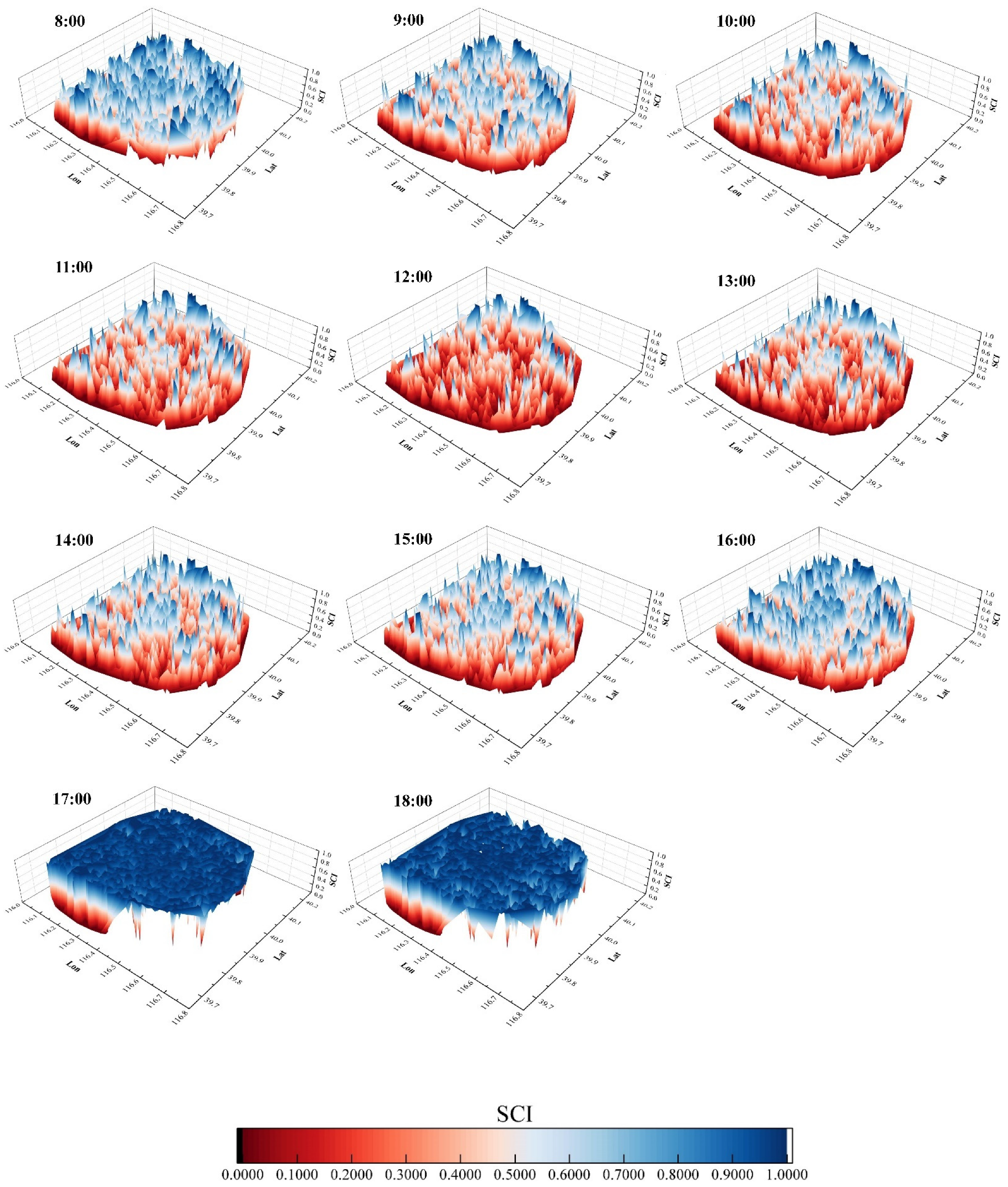
3.2.1. Diurnal and Spatial Distribution of Shading Coverage Index at 1-km Grid

The positions without panoramic images were excluded, and a total of 163,433 sample points were calculated in the entire study area. The model we used for feature migration can restore the density of the deciduous trees in winter to the dense segmentation results in summer, so we keep panoramas without leaves in winter. We map the site-level diurnal and spatial shadow areas at 1-h intervals on 1 August 2018. This study proposes an index to measure shadow intensity, that is, within a certain spatial range, the ratio of shadow area to all areas is defined as the shading coverage index at a certain moment. With the help of Equation (5), we draw the shading coverage index on a grid scale of 1 km based on the results of shadow points every 1 h and visualize it in three-dimension to explore the diurnal and spatial variation of shadow intensity. We set the specific spatial range as 1 km × 1 km, and 1 km × 1 km is the approximate average range of pedestrians in a city [44].

Figure 7 shows the distribution of the shading coverage index of the 1 km grid per hour from 8: 00 to 18:00. It can be found that the shading coverage index of the central region is higher than the periphery. Such a result is reasonable for the following reasons. First, the road network in the city center is denser (Figure 1), which results in more calculated samples and shadows. Secondly, in general, the areas with higher building density and plot ratio have greater shadow intensity, resulting in the shading coverage index value in the central area remaining at a high level. As can be seen from Figure 6 and Table 1 (right), from 10: 00 to 15:00, most of the cells in the study area are “red”, and the index value is between 0 and 0.4, indicating that more than half of the sample points are exposed to sunlight. The shading coverage index after 17:00 is significantly different from before. This has to do with sunsets, where the zenith angle of the sun at 17:00 and 18:00 is small to a certain angle, and most of the light is blocked by tall buildings and creates shadows. The solar zenith angle is the angle between the sun’s rays and the vertical [45]. As a result, the range of shadows is greatly increased. This situation is also verified in statistical data, as shown in

Table 2. The statistical values of shading coverage index.

Time	Scale of Road Section			Scale of 1 km Grid
	Average	Median	Standard Deviation	Average	Median	Standard Deviation
8:00	0.379	0.368	0.250	0.482	0.500	0.250
9:00	0.292	0.500	0.247	0.352	0.326	0.250
10:00	0.236	0.179	0.231	0.287	0.243	0.238
11:00	0.216	0.142	0.223	0.258	0.208	0.227
12:00	0.164	0.084	0.201	0.187	0.137	0.191
13:00	0.208	0.130	0.225	0.232	0.175	0.245
14:00	0.270	0.222	0.243	0.304	0.259	0.245
15:00	0.286	0.250	0.247	0.327	0.294	0.247
16:00	0.337	0.333	0.257	0.403	0.395	0.261
17:00	0.627	0.650	0.233	0.905	0.955	0.178
18:00	0.609	0.631	0.240	0.848	0.938	0.221

(right), and the shading coverage index at 16:00 had a mean of 0.403 and a median of 0.395. At 17:00, the mean and median shadow indices rose to 0.848 and 0.938, respectively.

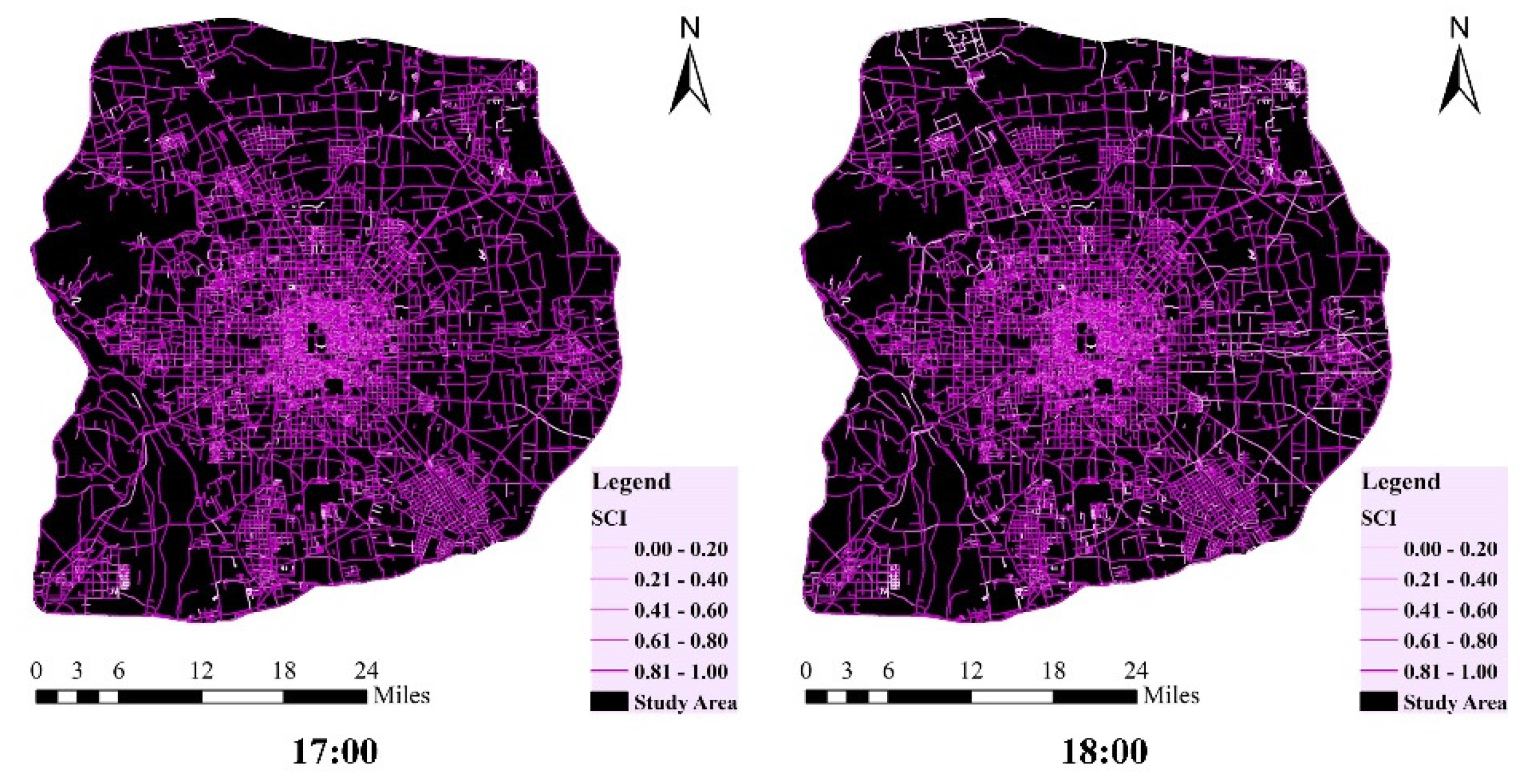
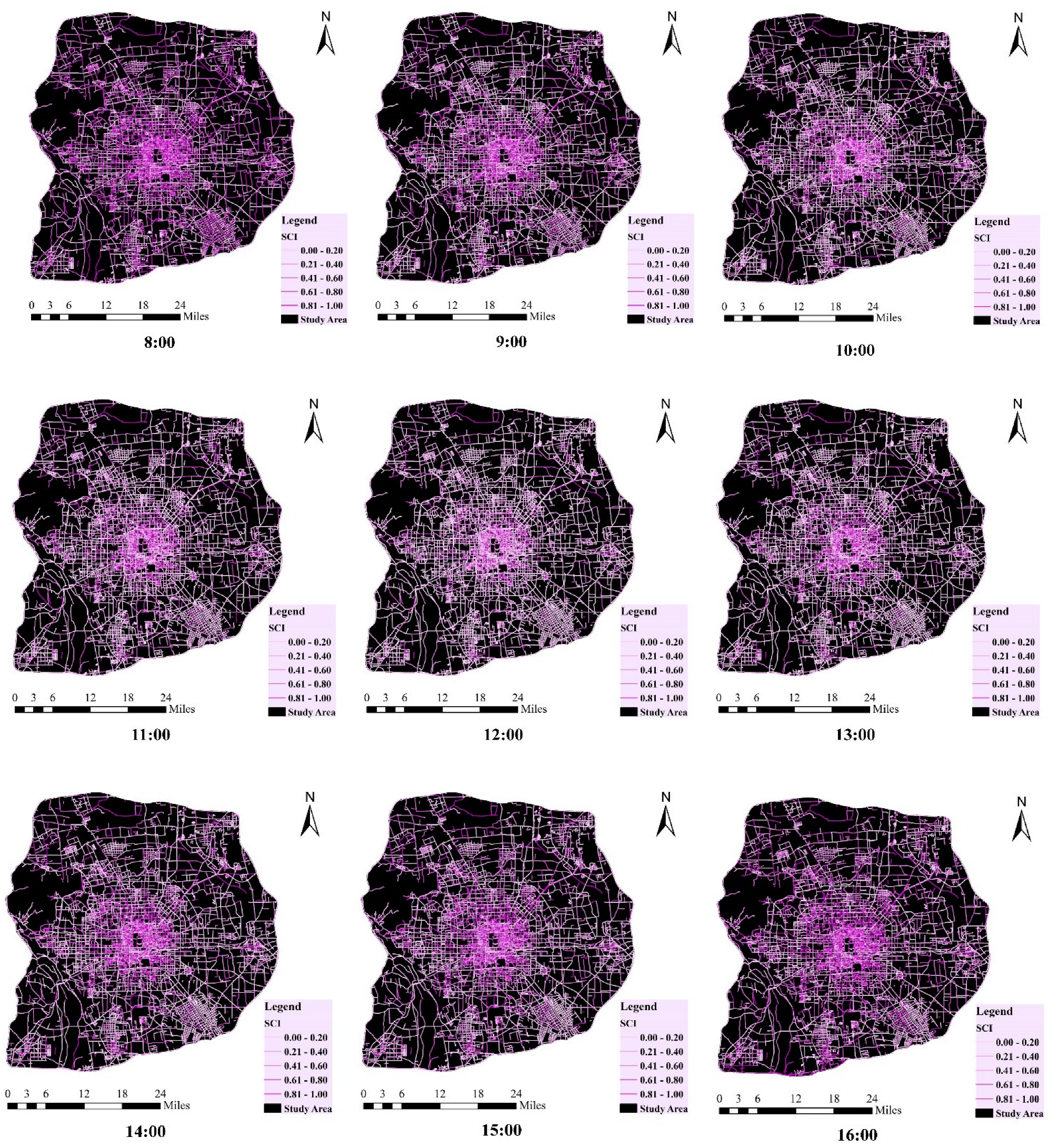
3.2.2. Diurnal and Spatial Distribution of Shading Coverage Index at the Scale of Road Section

The shading index can also be evaluated on the scale of road segments. The sample sites in the shadow at each moment are aggregated to the nearest road section, and then the number of sample sites in the shadow is divided by all the site numbers on that road section to represent the shading coverage index at the scale of a road section. Figure 8 shows the shading coverage index values of all road sections in the study area, calculated by Equation (5). From the visualization results, shadow coverage on the street decreases first and then increases during the day. The shading coverage index values are higher at 8:00–9:00 and 17:00–18:00 compared to other times. The zenith angles of the sun at 8:00 and 18:00 are 57.045° and 77.581°, respectively, and “dark pink” areas are more likely to appear in shadows from buildings and vegetation. When the solar zenith angle is low (such as 22.129°), the shading coverage index value of the building is small, and it blocks less light due to the upright nature of the building. Only the area under the vegetation canopy is shaded. As can be seen from the statistics in Table 2 (left), both the mean and median values of the shading coverage index are the smallest. The shading coverage index shows significant differences among the different grades of roads. A comparison of the different grades of roads shows that the shade index of highways and arterial roads is “lighter pink” than that of the slip roads because highways and urban arterial roads are generally wider than slip roads.

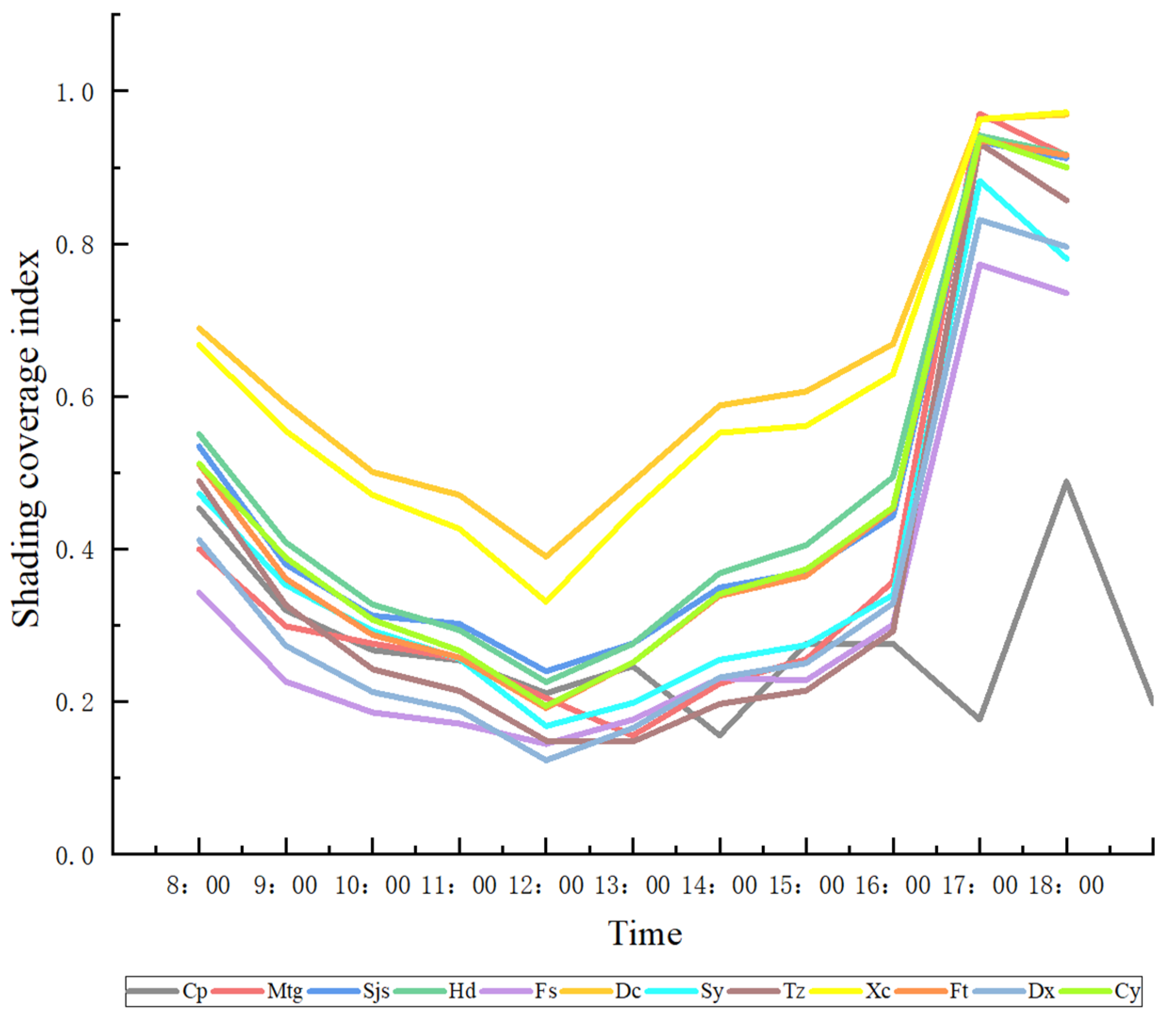
3.2.3. Shading Coverage Index at the Scale of Administrative District

Taking each administrative region of Beijing as a unit, we count the shading coverage index changes of each region over time, to test the shading coverage index distribution at the scale of the administrative district (Figure 9). The shading coverage index is significantly higher than other administrative regions in Dongcheng and Xicheng districts. These results are consistent with the results of the 1 km grid, indicating that the shading coverage index is higher in the central urban area than in the outer areas. The shading coverage index curve of Changping District is quite different from other administrative regions. This is because Changping District not only has relatively sparse roads but also has more streets in the east-west direction than in the north-south direction, and east-west streets are more likely to be exposed to direct sunlight between 17:00–18:00.

4. Discussion

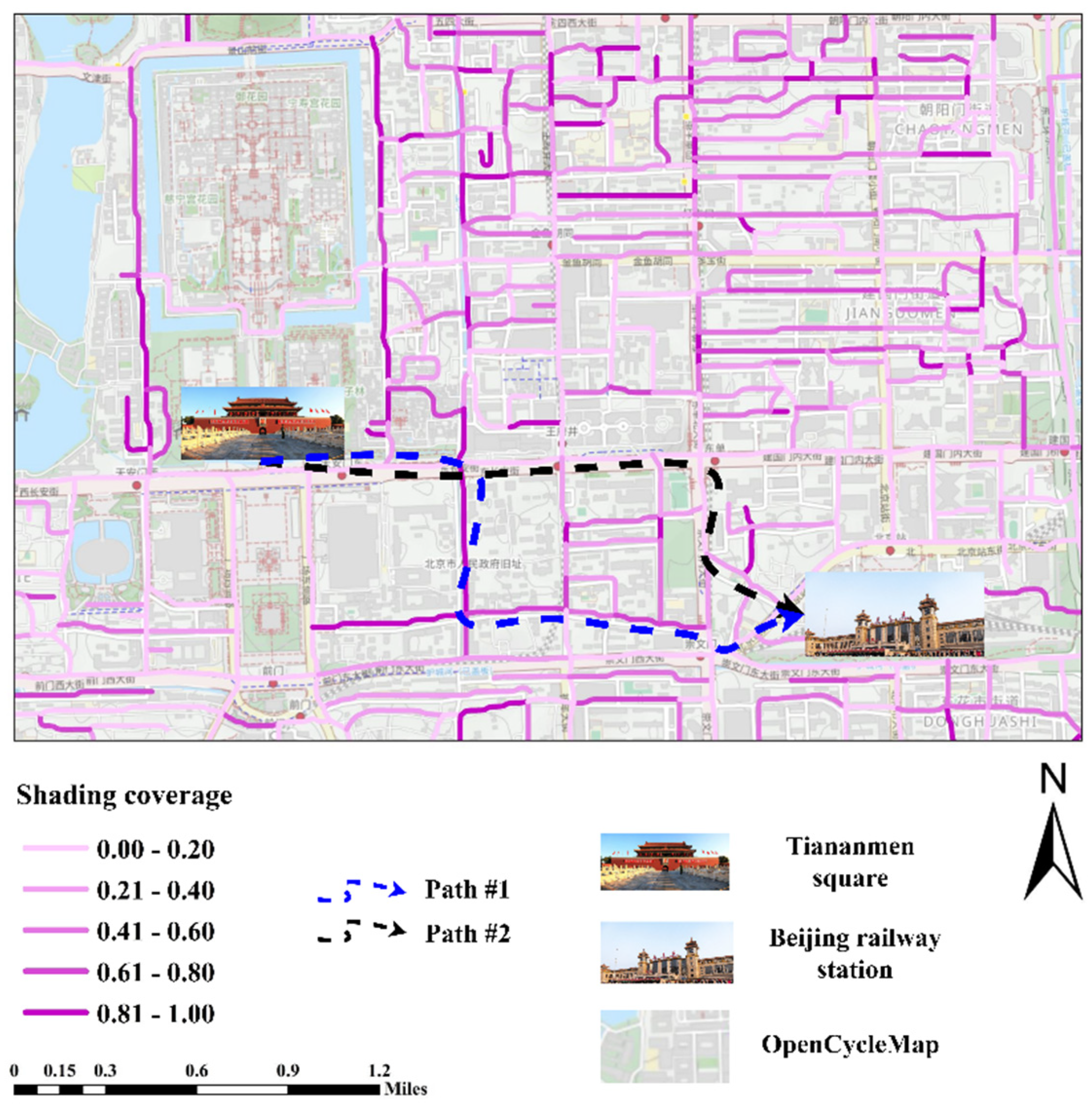
4.1. Shading Coverage Index Applications

In this current study, we explore a way of transferring street characteristics of the Cityscapes dataset to semantically segment street-level panoramic images of Beijing by using DeepLabv3+ and propose an effective and rapid method to quantify the diurnal and spatial changes in shadows. The research has the following characteristics. Firstly, being different from other deep learning-based methods, this study explores the feasibility and reliability of applying a deep learning transfer strategy in shadow mapping of urban street scenes. Therefore, on the basis of shadow mapping that meets certain requirements, we can save a lot of sample labeling and model training time costs compared with other non-transfer strategies. The shadow recognition method, which is based on feature migration applied in this research, can be transferred to other cities covered by street view images. The experimental results on the CamVid dataset have preliminarily confirmed this, with entirely new city scenes; the DeepLabv3+ model we selected responds well to the sky class (Table 1).

Secondly, this study provides an idea for estimating shadows from urban street panoramas to promote the development of related macro and micro research. The results of the grid scale and the administrative area scale are consistent with the research on the urban built environment structure, such as land use [46,47] and the distribution of street trees [48]. Moreover, our results on shading levels and changes can be verified from previous research results on the shading effect in local areas in Beijing [49]. For example, the shading changes of the Central Business District (CBD) in our results have the same spatial and diurnal laws as the research on the shading effect and radiation in the CBD based on remote sensing data sources [49,50]. From a macro perspective, the shading coverage distribution in a 1 km grid and administrative areas will help urban planners and managers to make relevant decisions. Urban planners and managers can determine greening schemes according to the shading coverage index and its distribution to further alleviate the urban heat island effect. This method can provide researchers in the fields of environment, health, tourism, transportation and urban planning with a method to quantify the characteristics of other urban shadows, helping them to complete related research faster and more efficiently. From a micro perspective, the diurnal and spatial distribution of shading coverage in road segments can be used for optimal route recommendations. According to our research results, when the shading coverage index at the grid scale of 1 km is higher than the corresponding road segment scale, it may mean that there are road segments with high shadow coverage within 1 km². The research shows that when alternative routes are available, such as the best shade route, the shortest route is not the best choice for pedestrians [51]. Distance and time are indeed important factors in determining route choice, but this choice is more dependent on the characteristics of other alternative routes [52]. Pedestrians are generally willing to take a safer, more comfortable, or more interesting route, as long as the chosen route remains within a reasonable range relative to the shortest route [53,54]. That is, the results of our method can help pedestrians find the shady route with the most shadow coverage between the starting point and the ending point, to obtain a better travel experience in hot weather.

To be specific, as shown in the figure below (Figure 10), we compare the shadow amount and shading coverage index with two paths at noon. Path #1 has a higher shadow amount and shading coverage index than Path #2, which is the shortest path. There are 36 and 8 sample sites in shadow for Path #1 and Path #2, respectively. The shading coverage indexes of Path #1 and Path #2 are 0.54 and 0.13, respectively. Additionally, Path #1 is about 230 m longer than Path #2. The results show that the path with a higher shading coverage index (Path #1) only requires pedestrians to travel 230 m more to add 28 shadow sites compared to the path with a shorter distance (Path #2). This means that the higher shading coverage index path provided in this research can guide pedestrians to select a more comfortable route, particularly, it can avoid too much harm to human beings caused by hot weather.

4.2. Limitations and Future Consideration

There are still some limitations that should be addressed in future applications. First, this method is only applicable to areas where BSV can be obtained and the majority of BSV panoramas analyzed in this study were taken in 2013, 2017, 2018, and 2020, which may lead to outdated data. Second, as this is a study on the quantity of shadows, no assessment of shadow quality can be derived from this study, for example, evaluating the light transmittance of different shading elements [55]. In the future, researchers can focus on the combination of the “quality” and “quantity” of shading. Future research can also combine multiple image data sources to mine shadow features that are not limited to urban streets.

5. Conclusions

This research proposes a novel and effective shadow estimation method, which designs an index to quantify the shadows of urban streets by exploring a method of using DeepLabv3+ to transfer street features in Cityscapes data to the semantic segmentation of street panoramic images in Beijing. Furthermore, the diurnal and spatial changes of shadow are visually displayed on different scales. The experimental results show that the diurnal and spatial consistency between the shadow estimation method based on deep feature transfer and the actual shadow distribution reaches 83%. The diurnal and spatial variation of the shading coverage index provides an important reference for evaluating the construction of shading facilities. Through experiments comparing the distribution of shadow indices in road sections, it is also proved that our method can provide an important basis for pedestrians to find routes with better shading conditions, thereby reducing harm to people in hot weather.

References

1. Jiang, C.; Ward, M.O. Shadow identification. In Proceedings of the 1992 IEEE Computer Society Conference on Computer Vision and Pattern Recognition, Champaign, IL, USA, 15–18 June 1992; pp. 606–612. [Google Scholar] [CrossRef]
2. Mehta, V. The Street: A Quintessential Social Public Space; Routledge: London, UK, 2013. [Google Scholar]
3. Zhou, W.; Wang, J.; Cadenasso, M.L. Effects of the spatial configuration of trees on urban heat mitigation: A comparative study. Remote Sens. Environ. 2017, 195, 1–12. [Google Scholar] [CrossRef]
4. Poumadère, M.; Mays, C.; Le Mer, S.; Blong, R. The 2003 heat wave in France: Dangerous climate change here and now. Risk Anal. 2005, 25, 1483–1494. [Google Scholar] [CrossRef] [PubMed]
5. Harlan, S.L.; Ruddell, D.M. Climate change and health in cities: Impacts of heat and air pollution and potential co-benefits from mitigation and adaptation. Curr. Opin. Environ. Sust. 2011, 3, 126–134. [Google Scholar] [CrossRef]
6. Ouillet, A.; Rey, G.; Laurent, F.; Pavillon, G.; Bellec, S.; Guihenneuc-Jouyaux, C.; Clavel, J.; Jougla, E.; Hemon, D. Excess mortality related to the August 2003 heat wave in France. Int. Arch. Occup. Environ. Health 2006, 80, 16–24. [Google Scholar] [CrossRef] [PubMed] [Green Version]
7. Sun, Q.C.; Macleod, T.; Both, A.; Hurley, J.; Butt, A.; Amati, M. A human-centered assessment framework to prioritise heat mitigation efforts for active travel at city scale. Sci. Total Environ. 2021, 763, 143033. [Google Scholar] [CrossRef] [PubMed]
8. Loughner, C.P.; Allen, D.J.; Zhang, D.; Pickering, K.E.; Dickerson, R.R.; Landry, L. Roles of urban tree canopy and buildings in urban heat island effects: Parameterization and preliminary results. J. Appl. Meteorol. Clim. 2012, 51, 1775–1793. [Google Scholar] [CrossRef]
9. Krier, R.; Rowe, C. Urban Space; Academy Editions: London, UK, 1979. [Google Scholar]
10. Chen, L.; Ng, E. Outdoor thermal comfort and outdoor activities: A review of research in the past decade. Cities 2012, 29, 118–125. [Google Scholar] [CrossRef]
11. Samarasekara, G.N.; Fukahori, K.; Kubota, Y. Environmental correlates that provide walkability cues for tourists: An analysis based on walking decision narrations. Environ. Behav. 2011, 43, 501–524. [Google Scholar] [CrossRef]
12. Li, X.; Yoshimura, Y.; Tu, W.; Ratti, C. A pedestrian-level strategy to minimize outdoor sunlight exposure. Artif. Intell. Mach. Learn. Optim. Tools Smart Cities 2022, 123–134. [Google Scholar] [CrossRef]
13. Kang, J.; Körner, M.; Wang, Y.; Taubenböck, H.; Zhu, X.X. Building instance classification using street view images. ISPRS J. Photogramm. 2018, 145, 44–59. [Google Scholar] [CrossRef]
14. Wang, J.; Tett, S.F.B.; Yan, Z. Correcting urban bias in large-scale temperature records in China, 1980–2009. Geophys. Res. Lett. 2017, 44, 401–408. [Google Scholar] [CrossRef] [Green Version]
15. Cao, Q.; Yu, D.; Georgescu, M.; Wu, J.; Wang, W. Impacts of future urban expansion on summer climate and heat-related human health in eastern China. Environ. Int. 2018, 112, 134–146. [Google Scholar] [CrossRef] [PubMed]
16. Nasrollahi, N.; Hatami, Z.; Taleghani, M. Development of outdoor thermal comfort model for tourists in urban historical areas; A case study in Isfahan. Build. Environ. 2017, 125, 356–372. [Google Scholar] [CrossRef]
17. Lubans, D.R.; Boreham, C.A.; Kelly, P.; Foster, C.E. The relationship between active travel to school and health-related fitness in children and adolescents: A systematic review. Int. J. Behav. Nutr. Phy. 2011, 8, 1–12. [Google Scholar] [CrossRef] [Green Version]
18. Rodríguez-Algeciras, J.; Tablada, A.; Matzarakis, A. Effect of asymmetrical street canyons on pedestrian thermal comfort in warm-humid climate of Cuba. Theor. Appl. Climatol. 2018, 133, 663–679. [Google Scholar] [CrossRef]
19. Shashua-Bar, L.; Hoffman, M.E. Vegetation as a climatic component in the design of an urban street: An empirical model for predicting the cooling effect of urban green areas with trees. Energy Build. 2000, 31, 221–235. [Google Scholar] [CrossRef]
20. Lin, T.; Tsai, K.; Hwang, R.; Matzarakis, A. Quantification of the effect of thermal indices and sky view factor on park attendance. Landsc. Urban Plan. 2012, 107, 137–146. [Google Scholar] [CrossRef]
21. Peng, F.; Xiong, Y.; Zou, B. Identifying the optimal travel path based on shading effect at pedestrian level in cool and hot climates. Urban Clim. 2021, 40, 100988. [Google Scholar] [CrossRef]
22. Muhaisen, A.S. Shading simulation of the courtyard form in different climatic regions. Build. Environ. 2006, 41, 1731–1741. [Google Scholar] [CrossRef]
23. Oke, T.R. Street design and urban canopy layer climate. Energy Build. 1988, 11, 103–113. [Google Scholar] [CrossRef]
24. White, M.; Hu, Y.; Burry, M.; Ding, W.; Langenheim, N. Cool City Design: Integrating Real-Time Urban Canyon Assessment into the Design Process for Chinese and Australian Cities. Urban Plan. 2016, 3, 25–37. [Google Scholar] [CrossRef]
25. Middel, A.; Lukasczyk, J.; Maciejewski, R. Sky View Factors from Synthetic Fisheye Photos for Thermal Comfort Routing—A Case Study in Phoenix, Arizona. Urban Plan. 2017, 2, 19–30. [Google Scholar] [CrossRef]
26. Carrasco-Hernandez, R.; Smedley, A.R.D.; Webb, A.R. Using urban canyon geometries obtained from Google Street View for atmospheric studies: Potential applications in the calculation of street level total shortwave irradiances. Energy Build. 2015, 340–348. [Google Scholar] [CrossRef]
27. Johansson, E.; Emmanuel, R. The influence of urban design on outdoor thermal comfort in the hot, humid city of Colombo, Sri Lanka. Int. J. Biometeorol. 2006, 51, 119–133. [Google Scholar] [CrossRef] [PubMed]
28. Moro, J.; Krüger, E.L.; Camboim, S. Shading analysis of urban squares using open-source software and free satellite imagery. Appl. Geomat. 2020, 12, 441–454. [Google Scholar] [CrossRef]
29. Chen, X.; Zhao, H.; Li, P.; Yin, Z. Remote sensing image-based analysis of the relationship between urban heat island and land use/cover changes. Remote Sens. Environ. 2006, 104, 133–146. [Google Scholar] [CrossRef]
30. Klemm, W.; Heusinkveld, B.G.; Lenzholzer, S.; van Hove, B. Street greenery and its physical and psychological impact on thermal comfort. Landsc. Urban Plan. 2015, 138, 87–98. [Google Scholar] [CrossRef]
31. Chow, A.; Fung, A.; Li, S. GIS Modeling of Solar Neighborhood Potential at a Fine Spatiotemporal Resolution. Buildings 2014, 4, 195–206. [Google Scholar] [CrossRef]
32. Du, K.; Ning, J.; Yan, L. How long is the sun duration in a street canyon? Analysis of the view factors of street canyons. Build. Environ. 2020, 172, 106680. [Google Scholar] [CrossRef]
33. Gong, F.; Zeng, Z.; Zhang, F.; Li, X.; Ng, E.; Norford, L.K. Mapping sky, tree, and building view factors of street canyons in a high-density urban environment. Build. Environ. 2018, 134, 155–167. [Google Scholar] [CrossRef]
34. Liu, Y.; Zhang, M.; Li, Q.; Zhang, T.; Yang, L.; Liu, J. Investigation on the distribution patterns and predictive model of solar radiation in urban street canyons with panorama images. Sustainable Cities Soc. 2021, 75, 103275. [Google Scholar] [CrossRef]
35. Li, X.; Ratti, C. Mapping the spatio-temporal distribution of solar radiation within street canyons of Boston using Google Street View panoramas and building height model. Landsc. Urban Plan. 2019, 191, 103387. [Google Scholar] [CrossRef]
36. Yang, J.; Yi, D.; Qiao, B.; Zhang, J. Spatio-temporal change characteristics of spatial-interaction networks: Case study within the sixth ring road of Beijing, China. ISPRS Int. J. Geo-Inf. 2019, 8, 273. [Google Scholar] [CrossRef] [Green Version]
37. Dong, R.; Zhang, Y.; Zhao, J. How green are the streets within the sixth ring road of Beijing? An analysis based on Tencent Street View pictures and the Green View Index. Int. J. Environ. Res. Public Health 2018, 15, 1367. [Google Scholar] [CrossRef] [PubMed] [Green Version]
38. Chen, X.; Meng, Q.; Hu, D.; Zhang, L.; Yang, J. Evaluating Greenery around Streets Using Baidu Panoramic Street View Images and the Panoramic Green View Index. Forests 2019, 10, 1109. [Google Scholar] [CrossRef] [Green Version]
39. Chen, L.; Zhu, Y.; Papandreou, G.; Schroff, F.; Adam, H. Encoder-Decoder with strous separable convolution for semantic image segmentation. In Proceedings of the European Conference on Computer Vision (ECCV), Munich, Germany, 8–14 September 2018. [Google Scholar] [CrossRef] [Green Version]
40. Cordts, M.; Omran, M.; Ramos, S.; Scharw Achter, T.; Enzweiler, M.; Benenson, R.; Franke, U.; Roth, S.; Schiele, B. The Cityscapes Dataset; CVPR Workshop on the Future of Datasets in Vision: New Orleans, LO, USA, 2015. [Google Scholar]
41. Chouai, M.; Dolezel, P.; Stursa, D.; Nemec, Z. New End-to-End Strategy Based on DeepLabv3+ Semantic Segmentation for Human Head Detection. Sensors 2021, 21, 5848. [Google Scholar] [CrossRef] [PubMed]
42. He, X.D.; Shen, S.H.; Miao, S.G. Applications of fisheye imagery in urban environment: A case based study in Nanjing. Adv. Mater. Res. 2013, 726, 4870–4874. [Google Scholar] [CrossRef]
43. Yousuf, M.U.; Siddiqui, M.; Rehman, N.U. Solar energy potential estimation by calculating sun illumination hours and sky view factor on building rooftops using digital elevation model. J. Renew. Sustain. Energy 2018, 10, 13703. [Google Scholar] [CrossRef]
44. Forsyth, A. What is a walkable place? The walkability debate in urban design. Urban Des. Int. 2015, 20, 274–292. [Google Scholar] [CrossRef]
45. Jacobson, M.Z. Fundamentals of Atmospheric Modeling; Cambridge University Press: Cambridge, UK, 1999. [Google Scholar]
46. Li, X.; Hu, T.; Gong, P.; Du, S.; Chen, B.; Li, X.; Dai, Q. Mapping Essential Urban Land Use Categories in Beijing with a Fast Area of Interest (AOI)-Based Method. Remote Sens. 2021, 13, 477. [Google Scholar] [CrossRef]
47. Zhang, Y.; Li, Q.; Huang, H.; Wu, W.; Du, X.; Wang, H. The Combined Use of Remote Sensing and Social Sensing Data in Fine-Grained Urban Land Use Mapping: A Case Study in Beijing, China. Remote Sens. 2017, 9, 865. [Google Scholar] [CrossRef] [Green Version]
48. Zhao, S.; Tang, Y.; Chen, A. Carbon Storage and Sequestration of Urban Street Trees in Beijing, China. Front. Ecol. Evol. 2016, 4, 53. [Google Scholar] [CrossRef] [Green Version]
49. Ma, B.C.; Sang, Q.; Gou, J.F. Shading Effect on Outdoor Thermal Comfort in High-Density City a Case Based Study of Beijing. Adv. Mater. Res. 2014, 1065–1069, 2927–2930. [Google Scholar] [CrossRef]
50. Guo, Z.; Zhang, Z.; Wu, X.; Wang, J.; Zhang, P.; Ma, D.; Liu, Y. Building shading affects the ecosystem service of urban green spaces: Carbon capture in street canyons. Ecol. Model. 2020, 431, 109178. [Google Scholar] [CrossRef]
51. Guo, Z.; Loo, B.P.Y. Pedestrian environment and route choice: Evidence from New York City and Hong Kong. J. Transp. Geogr. 2013, 28, 124–136. [Google Scholar] [CrossRef]
52. Hoogendoorn, S.P.; Bovy, P.H.L. Pedestrian route-choice and activity scheduling theory and models. Transp. Res. Part B Methodol. 2004, 38, 169–190. [Google Scholar] [CrossRef]
53. Sevtsuk, A.; Basu, R.; Li, X.; Kalvo, R. A big data approach to understanding pedestrian route choice preferences: Evidence from San Francisco. Travel Behav. Soc. 2021, 25, 41–51. [Google Scholar] [CrossRef]
54. Xue, P.; Jia, X.; Lai, D.; Zhang, X.; Fan, C.; Zhang, W.; Zhang, N. Investigation of outdoor pedestrian shading preference under several thermal environment using remote sensing images. Build. Environ. 2021, 200, 107934. [Google Scholar] [CrossRef]
55. Peeters, A.; Shashua-Bar, L.; Meir, S.; Shmulevich, R.R.; Caspi, Y.; Weyl, M.; Motzafi-Haller, W.; Angel, N. A decision support tool for calculating effective shading in urban streets. Urban Clim. 2020, 34, 100672. [Google Scholar] [CrossRef]
Figure 1. The study area and its road network. Sjs, Dc and Xc are the abbreviations for the administrative districts of Shijingshan, Dongcheng and Xicheng, respectively.
Remotesensing 14 01796 g001
Figure 2. Schematic framework of this study.
Remotesensing 14 01796 g002
Figure 3. DeepLabv3+ semantic segmentation network structure.
Remotesensing 14 01796 g003
Figure 4. Transformation of cylindrical panoramic image to azimuthal fisheye image. (a) Top half of panorama image. (b) Schematic diagram of cylindrical projection. (c) Schematic diagram of azimuthal projection. (d) Fisheye image based on azimuth projection.
Remotesensing 14 01796 g004
Figure 5. The path of the sun is superimposed on a fisheye image in Beijing (1st August 2018). (a) Fisheye image based on semantic segmentation results. (b) Fisheye image after overlaying the sun’s path.
Remotesensing 14 01796 g005
Figure 6. Comparison of our predicted results with the BSV data.
Remotesensing 14 01796 g006
Figure 7. The three-dimensional map of shading coverage index in the 1 km grid. The x- and y-axes, respectively, represent the latitude and longitude, the z-axis represents the value of shading coverage index.
Remotesensing 14 01796 g007
Figure 8. Spatial and diurnal distribution of shading coverage index at the scale of road section.
Remotesensing 14 01796 g008aRemotesensing 14 01796 g008b
Figure 9. Line chart of shading coverage index for each administrative region. Each abbreviation means the following: Cp (Changping), Mtg (Mentougou), Sjs (Shijingshan), Hd (Haidian), Fs (Fangshan), Sy (Shunyi), Tz (Tongzhou), Xc (Xicheng), Ft (Fengtai), Dc (Dongcheng), and Cy (Chaoyang).
Remotesensing 14 01796 g009
Figure 10. Comparison of shadow indices of different paths.
Remotesensing 14 01796 g010