A Dilated Segmentation Network with the Morphological Correction Method in Farming Area Image Series

Abstract

Farming areas are made up of diverse land use types, such as arable lands, grasslands, woodlands, water bodies, and other surrounding agricultural architectures. They possess imperative economic value, and are considerably valued in terms of farmers’ livelihoods and society’s flourishment. Meanwhile, detecting crops in farming areas, such as wheat and corn, allows for more direct monitoring of farming area production and is significant for practical production and management. However, existing image segmentation methods are relatively homogeneous, with insufficient ability to segment multiple objects around the agricultural environment and small-scale objects such as corn and wheat. Motivated by these issues, this paper proposed a global-transformer segmentation network based on the morphological correction method. In addition, we applied the dilated convolution technique to the backbone of the model and the transformer technique to the branches. This innovation of integrating the above-mentioned techniques has an active impact on the segmentation of small-scale objects. Subsequently, the backbone improved by this method was applied to an object detection network based on a corn and wheat ears dataset. Experimental results reveal that our model can effectively detect wheat ears in a complicated environment. For two particular segmentation objects in farming areas, namely water bodies and roads, we notably proposed a morphological correction method, which effectively reduces the number of connected domains in the segmentation results with different parameters of dilation and erosion operations. The segmentation results of water bodies and roads were thereby improved. The proposed method achieved 0.903 and 13 for $mIoU$ and continuity. This result reveals a remarkable improvement compared with the comparison model, and the continuity has risen by 408%. These comparative results demonstrate that the proposed method is eminent and robust enough to provide preliminary preparations and viable strategies for managing farming area resources and detecting crops.

1. Introduction

In the 21st century, the population is increasing, and the rapid growth of human society has consumed numerous natural resources and seriously contaminated the environment. In order to coordinate the relationship between the strikingly rapid development rate and environmental resources of farming areas, and to continuously improve human living standards and carry out sustainable development, we must monitor and protect the environmental resources of farming areas at four levels: (1) Arable land—ensuring the quantity and quality of arable land is of primary importance for maintaining sustainable agricultural development [1]. (2) Grassland [2]—grassland is a renewable natural resource that covers about 1/2 of the total global land area, and is the most fundamental means of production and base for developing grassland livestock farming. (3) Woodland—woodland is an integral component of forest resource assets, and the source of forest material production and ecological services [3], whose area and value are mainly evaluated when conducting economic benefits assessment. (4) Water—human economic flourishment and agricultural production, including hydroelectric power generation, irrigation, shipping, fisheries, also rely on water. Each of these four levels can be monitored and protected with the assistance of computer technology.

Thanks to the prosperous trends in computer technology in the remote sensing field, enormous technical support has been provided for remote monitoring and protection of farming areas in the field of computer vision. M. H. Elagouz et al. [4] used satellite data and remote sensing techniques to detect and supervise the transformation of land use or cover in the Egyptian Nile Delta. Willians Ribeiro Mendes et al. [5] intended to create an intelligent fuzzy inference system underlying precise irrigation knowledge. They ultimately established a system aiming to construct particular maps to manipulate the rotation speed of the central pivot, and satellite images were employed. Karim Ennouri et al. [6] suggested that due to the evolution of remote sensing technologies, satellite information has been regarded as the primary data source to monitor high-dimension crop growth conditions. In addition, the emergence of digital image processing methods have also made crop condition observation and decision-making straightforward.

Among the above techniques, aerial image segmentation is of particular interest in the agricultural research space. Previous scholars in this field have laid a solid foundation and achieved remarkable breakthroughs. To perform a fig plant segmentation in top-view RGB (red, green, blue) images, Jorge Fuentes-Pacheco et al. [7] proposed an encoder–decoder convolutional neural network (CNN) that classifies each pixel as crop or non-crop. They introduced the approach to the research institution and performed it on an aerial image dataset. The new network achieved an average accuracy of 93.85%. A manual ground truth segmentation with pixel precision was adopted to compare different algorithms. Satoki Tsuichihara et al. [8] created a farm management system that used aerial images of grass to detect weeds and precisely determine the quantity and location for applying fertilizers. Broad-leaved weeds may be detected with an accuracy of roughly 80% using a region segmentation method based on deep learning. Cow groups and locations can be located with higher volumes of cow manure by comparing the GPS data from the overall sensors. Maximilian Johenneken et al. [9] suggested an autonomous system to detect and categorize the cause of damage to grasslands. The strategy entailed using CNN for the semantic segmentation of grasslands. They constructed an RGB baseline and evaluated multimodal architectures, resulting in a joint representation of elevation information and spectrum. Experimental results demonstrate that incorporating late fusion with elevation features enriches the network’s all-around performance over the RGB baselines. Weitao Wang, Qin Ma et al. [10] validated the merits of combining multi-spectral (MS) and synthetic aperture radar (SAR) data to enhance classification accuracy, particularly in fog and cloud obscured areas. Additionally, they proposed an adaptive feature fusion method based on an attention mechanism and experimented with two patch construction methodologies. Experiments revealed that the suggested method with single-size patches produced the most favorable outcomes—a 0.91 average f1-score and 93.12% accuracy, to be exact. These outcomes suggested that by incorporating MS and SAR data with appropriate feature fusion methods, full-time and all-weather remote sensing monitoring of grassland resources is conceivable, effectively enhancing the self-adjusting capability of grasslands.

Even though the merits of progress and relatively high efficiency by current aerial image segmentation strategies are noticeable, they tend to be restricted to ideal circumstances, such as the desired premise with high-qualified aerial images. In other words, there are still various obstacles in this field.

1.

Multi-scale problem: one object in the image may occupy different frame sizes caused by the distance between the camera and the shooting object. The problem of multiple poses (or multiple perspectives) of the object is caused by the different shooting angles. External lighting conditions and weather would cause poor image quality and illuminance.

2.

Adjacent pixels are too similar to the image information in the receptive field (adjacent pixels are just on the boundary of the desired segmentation area), resulting in oscillation and distortion of the edges of the corresponding segmentation area.

3.

Pixel imbalance in different categories or instances in the same image is another barrier. The difficulty of segmenting different objects is not the same.

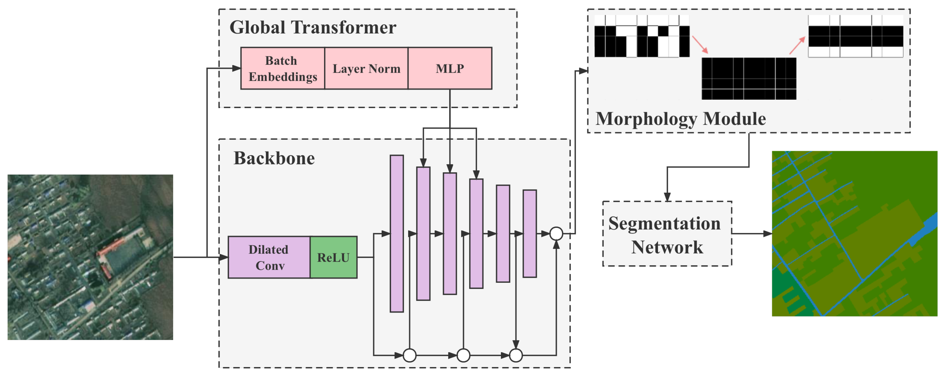
Driven by these preliminary requirements and relevant research in this area, this paper proposes a global farming area segmentation network using a morphological method to perform segmentation of farming areas (such as arable land, grasslands, woodlands, etc.) in aerial images, thereby resolving the aforementioned issues in the management of farming area resources. The principal contributions in this paper are as follows:

1.

The global-transformer structure was proposed to simplify the number of transformer parameters while retaining its core ability to extract global features.

2.

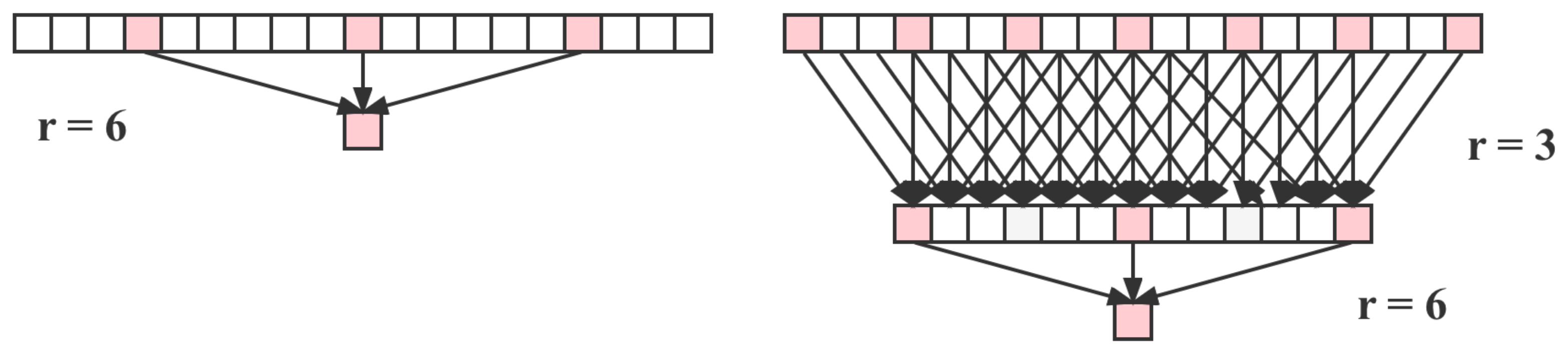
Applying dilated convolutional layers to the backbone further improves the segmentation capability of small-scale objects.

3.

A morphological method was used to reduce the number of connected domains for segmenting water bodies and roads in farming areas, so the segmentation effect could be as smooth and coherent as possible, with reduced noise.

Apart from these prominent contributions, limitations also exist in this study. (1) The road category—which retains comparatively the worst segmentation effect in the dataset—has a narrow shape in images, resulting in comprehensive model performance degradation. (2) The optimized segmentation performance of road categories is still insufficient, even though a separate model was selected. (3) Superior segmentation outcomes are based on an exceptional recognition rate. These limitations are future difficulties that the authors of this paper will strive to break through, and are the focus of subsequent research.

The subsequent sections of this paper are organized as follows: (1) The Related Work section demonstrates the preliminary theories and knowledge in the relative research field. (2) The Materials and Methods section describes the dataset and methods we employed, including the data pre-processing. (3) Important metrics, functions, settings, and training strategies are discussed in the Experiment section. (4) The Results and Discussion section illustrates the experimental results and provides a comparison. (5) The Conclusions section summarizes this study.

2. Related Work

Deep convolutional neural networks have been evolving, bringing continuous breakthroughs in image classification tasks. These models can integrate low, medium, or high-level features and then perform end-to-end classification, and the level of features can be enriched by applying deeper models. It is universally acknowledged that the effectiveness of a neural network is strongly related to the number of layers. In general, taking AlexNet [11,12] and VGG [13,14] as examples, the deeper the network, the better the results and the more difficult it is to train.

In contrast, the network’s training cost grows drastically as the depth rises further, while the results do not improve or even degrade. To resolve this issue, the deep residual learning framework ResNet [15] was proposed, with deeper network layers, more straightforward optimization, and more excellent training results corresponding to the depth.

However, training a deep model is much more complicated than designing a deep model, such as the gradient instability problems. Fortunately, these issues have been tackled to some extent by regularization, allowing networks with tens of layers to converge by stochastic gradient descent (SGD) [16] and backward propagation (BP) algorithms.

Another problem is that when deeper layers are able to converge, the accuracy of the network starts to plunge substantially. This degradation is not related to overfitting and brings about a more significant training error. This obstacle indicates that not all models are easy to train, and that shallow models may work better than deeper models that simply repeat the model’s layer.

Based on these excellent backbones, multiple segmentation networks were presented. We refer to the task with only one label (merely distinguishing categories) as semantic segmentation [17]. With regard to distinguishing different individuals of the same category, we refer to this as instance segmentation [18]. Since instance segmentation often only discriminates countable targets, the concept of panoptic segmentation was proposed by Alexander Kirillov et al. [19] in 2019 to realize both instance segmentation and semantic segmentation. Currently, the majority of the successful algorithms in image segmentation derive from the same pioneer: the fully convolutional network (FCN) suggested by Long et al. [20]. The FCN converts classification networks into a network structure for segmentation tasks and demonstrates that the segmentation problem can be implemented end-to-end in network training. For instance, the structure of UNet [21] is a U-shaped structure for encoding (downsampling) and then decoding (upsampling), keeping the input and output sizes the same. SegNet [22] is somewhat similar to UNet. It adopts an encoding–decoding structure. Such a structure mainly utilizes deconvolution and up-pooling. The decoder achieves nonlinear upsampling by pooling index, calculated by the maximum pooling operation of the encoder corresponding to the decoder.

The parameters in the backbones and segmentation networks are adjusted and optimized by the loss function. In regard to the different sorts of loss functions, softmax loss (cross-entropy loss with softmax) is the most common loss function in deep learning, which consists of three components: a fully connected layer, softmax function, and cross-entropy loss. The pipeline of softmax loss is as follows: first, an encoder is used to learn the features of the data, followed by the use of a fully connected layer, the softmax function, and finally cross-entropy is used to calculate the loss. More loss functions were proposed for different research areas and particular problems. For instance, the DIC loss function, an ensemble similarity measure function, is popularly used in medical image segmentation. Moreover, the BCE loss function creates a criterion that measures the binary cross entropy between the target and the input probabilities. In this study, we incorporated the Lovasz softmax loss and softmax loss and employed this combination.

3. Materials and Methods

3.1. Materials

3.1.1. Dataset Analysis

The dataset employed in this paper is from the Baidu Remote Sensing Image Parcel Segmentation Contest. It is divided into two categories, a training set and an A/B test set, where the training data set contains 140,000 images with a resolution of $256\times 256$ in jpg format. The A/B test set is derived from homogeneous images, where A possesses 10,000 images and B retains 20,000 images. The test set A is adopted for model evaluation in the evaluation stage, and the ultimate model performance is subject to the results of test set B.

The segmentation method used in this paper is also based on the 7:1:2 ratio commonly used in computer vision training strategies. Specifically, nearly 70% of the data are used for model training, 10% for evaluation, and 20% for testing to determine the final model performance. This ratio is adopted for segmentation because the model requires a large amount of data for training and a small amount of data for evaluation and testing.

As

Table 1. Dataset distribution details.

Class	Label	Percent
Buildings	0	2.79
Arable lands	1	50.87
Woodlands	2	17.87
Water body	3	17.74
Roads	4	0.35
grasslands	5	1.96
Others	6	7.38
Unlabeled	255	1.03

depicts, there is a noticeable category imbalance in the training data, such as buildings, roads, and grasslands, which account for 2.79%, 0.35%, and 1.96%, respectively. In contrast, the single category of arable land accounts for more than 50%. It is also apparent from the pre-training and validation of the baseline models that all models have meager recognition rates in terms of the roads and grasslands categories. Therefore, resolving the issue of data imbalance between categories significantly impacts the performance of the subsequent models.

3.1.2. Data Preprocessing

With regard to the pre-processing, the training images were normalized; in terms of data enhancement, image flipping and zoom enhancement approaches were applied in accordance with the rotation invariance of remote sensing images, as displayed in Figure 1.

Specifically, image enhancement has the following four roles:

1.

Avoid overfitting. When the dataset has some distinctive features, for example, when the images in the dataset are basically taken from the same scene, using related methods such as neural style transfer can avoid the model learning information that is irrelevant to the target.

2.

Improve the model’s robustness and reduce the sensitivity towards images. When the training data are in a comparatively ideal state and encounter some exceptional cases, such as occlusion, brightness, blur, etc., it is prone to misidentification. Hence, adding noise and mask to the training data is essential to improve the model’s robustness.

3.

Expand training data and thereby enhance the model’s generalizability.

4.

Take the employed dataset in this paper as an example; the extreme imbalance between positive and negative samples is prone to particular pattern recognition problems. Some data enhancement methods for fewer samples have a favorable influence on tackling the uneven proportion issue of samples.

In this paper, after applying the above simple data enhancement method implemented by an affine transformation, more complex data enhancement methods were also carried out. The reason for this attempt is to further improve the model’s performance. In Section sec: discussion_aug, we will explicitly compare the changes in model performance when different data augmentation methods are applied.

1.

Remote Erasing. This method is adapted from [23], similar to Cutout [24]. More specifically, remote erasing utilizes random pixels to fill a random-sized mask area, while Cutout uses fixed pixels to fill a square mask area. The remote erasing process is illustrated in Algorithm 1.

Algorithm 1 Remote erasing process

1: Input: Image I; Erasing probability p; 2: Output: Erased image $I^{*}$; 3: Initialization:$p_1$ 4: if$p_1<p$then 5:    $I_e=RandArea$ 6:    $I\left(I_e\right)=RandColor$ 7:    $I^{*}=I$ 8:    return $I^{*}$ 9: end

2.

Puzzle Block. The core idea of this method lies in dividing the image into $s\times s$ lattices, and each lattice is masked with a certain probability, say 0.5. Inevitably, a tiny target will be wholly masked out.

3.

Stockade Mask. This method co-opted GridMask [25] and FenceMask [26]. Compared with the above two methods, the proposed stockade mask method is more fine-grained, preventing the square and large-grained masks from irreversibly affecting the small targets.

Figure 2 exhibits the visualization of these data enhancement methods mentioned above.

3.2. Methods

3.2.1. Overview

This paper proposed a transformer-based global feature extraction method to better segment objects at different scales in farming areas aerial images, such as arable lands and water bodies, and improve remote sensing images’ anti-interference capability. Compared with other segmentation network models, our method possesses the following innovations:

1.

The global-transformer branch is added to the backbone to extract the global features, which is especially valuable for the segmentation of small-scale objects;

2.

In order to reduce the number of connected domains in the segmentation results, a morphological correction module is added after the segmentation network to evaluate the connectivity of objects such as water bodies and roads in farming area images.

The overall framework of the model is shown in Figure 3.

3.2.2. Global Transformer

The transformer has been modified to simplify the structure and reduce the number of network parameters. Meanwhile, it still has the potential to provide effective global feature extraction capability [27], which provides an idea of how to adapt the transformer network to small data size. Nevertheless, there are still some drawbacks in this study, such as: in simplifying the structure of the transformer, the number of parameters is declined, but at the same time, the global feature extraction ability of this structure is also decreased; in Gansformer [27], the transformer is still used for processing ultra-high resolution images, but how to apply it to small-scale images is still unknown.

Based on the above analysis, this paper further simplified the network structure based on the parallel structure of the transformer. As Figure 3 depicts, in order to offset the massive number of parameters, the considerable training set corresponding to these parameters, and the exponential increase in training time, we retained only the encoder and decoder employed by the transformer to extract global features. This change would inevitably reduce feature extraction capability, so this paper applied the dilated convolution to the backbone. The primary purpose is to provide global feature extraction capability in the transformer branch and obtain a larger scale of the receptive field in the backbone with fewer parameters, i.e., global feature extraction capability.

3.2.3. Dilated Pyramid Backbone

As can be seen in Figure 3, the dilated pyramid backbone can be divided into two parts: dense porous spatial pyramidal pooling with dense atrous spatial pyramid pooling and spatial convolutional neural network. The former fuses the input and output of the small sampling rate cavity convolution layer. It then inputs the fused features into the subsequent cavity convolution layer with a large sampling rate to obtain dense multi-scale contextual information. The latter is based on the former, and each output is spatially convolved in different directions to capture more dense multi-scale contextual information. Therefore, the proposed semantic segmentation method further improves the accuracy of the segmentation results by capturing richer contextual information.

The dilated pyramid backbone can effectively increase the receptive field of the convolution kernel, which is calculated as Equation (1) shows, where R denotes the size of the receptive field, k denotes the size of the convolution kernel, and r denotes the size of the sampling rate.

$$R=(r-1)\times (k-1)+k$$

(1)

Stacking two dilated convolution layers can produce a larger range of receptive fields, assuming that the receptive field sizes of the two-cavity convolution layers are $R_1$ and $R_2$, respectively. The size of the receptive field $R_{new}$ is then produced after stacking is shown in Equation (2).

$$R_{new}=R_1+R_2-1$$

(2)

The dilated pyramid backbone includes more valid pixel information in the computation of the feature map than the ASPP model. That is because the ASPP uses a large sampling rate of the atrous convolution to convolve the feature map with very sparse pixels, compared to the standard convolution with the same receptive field.

Figure 4 shows the effect of different structures of the dilated convolution layer on pixel sampling. The left panel shows the ASPP structure with a single dilated convolution layer of sampling pixels of a one-dimensional signal, with a convolution kernel size of three and a sampling rate of six. Moreover, the sampling rates are three and six, respectively. The figure on the right shows the pixel sampling of a one-dimensional signal in the dilated pyramid structure using a stack of two dilated convolution layers, both with a convolution kernel size of three and sampling rates of three and six, respectively.

Table 2. Different combinations of sampling rates.

Sampling Rates	Size of Receptive Field
3	7
6	13
12	25
18	37
6, 12	37
3, 6, 12	43
3, 12, 18	67
3, 6, 12, 18	79

shows the receptive field size for different combinations of sampling rates.

3.2.4. Morphology Module

This paper improved the connectivity to improve the model’s segmentation effect for narrow objects like water bodies and roads. We introduced the morphology module after the segmentation network. This module is mainly responsible for two processing tasks: one is to perform the morphology closure operation, dilation, and then erosion, and set different dilation and erosion coefficients, respectively, to obtain the connectivity effect; on the other hand, it removes the tiny area noise.

Figure 5A illustrates that the initial segmentation result of roads is unsatisfactory, and a large number of unconnected regions and pixel blocks are generated.

By expanding these discrete regions to form a completed connected domain and then eroding them, both the discrete segmented regions are connected, and the segmentation results are restored by erosion. Figure 6A,B demonstrate the visualization of the morphology module dilation and erosion of the original segmentation result.

Figure 6B, meanwhile, reflects that the small noise in the segmentation result can be removed by adjusting the coefficient of dilation and erosion, more specifically, rendering the erosion coefficient more considerable than the dilation coefficient. The slight noise at the markers is removed by a slight dilation and a more effective erosion operation. Figure 5B indicates the optimization effect of applying the above principle to the segmentation results on this dataset.

4. Experiment

4.1. Evaluation Metrics

The semantic segmentation task is essentially a classification task, where the object of classification is each pixel in the input image. Therefore, when evaluating the performance of a semantic segmentation task, the relevant performance metric of the classification task is frequently utilized. More specifically, depending on the combination of the actual and predicted categories of the classification objects, four classification results will be obtained. Each of these four combinations yields $TP$ (True Positive), when the predicted result is the same as the true label, and others, $FP$ (False Positive), $FN$ (False Negative) and $TN$ (True Negative), as shown in

Table 3. Confusion matrix of classification indicators.

		Ground Truth
		Positive	Negative
Prediction	Positive	TP	FP
	Negative	FN	TN

. This table is only used to indicate how the above four parameters are defined, not to indicate the specific values of these parameters.

where Positive represents the positive sample, while Negative represents the negative sample. $TP$ denotes that the actual category of the sample is positive, and the predicted category is also positive, alleged “True Positive”. $FP$ denotes that the actual category of the sample is negative, whereas the predicted category is positive, entitled “False Positive”. $FN$ indicates that the actual category of the sample is positive, but the predicted category is negative, alleged “False Negative”. $TN$ means that the actual category of the sample is negative; meanwhile, the predicted category is also negative, which is called “True Negative”.

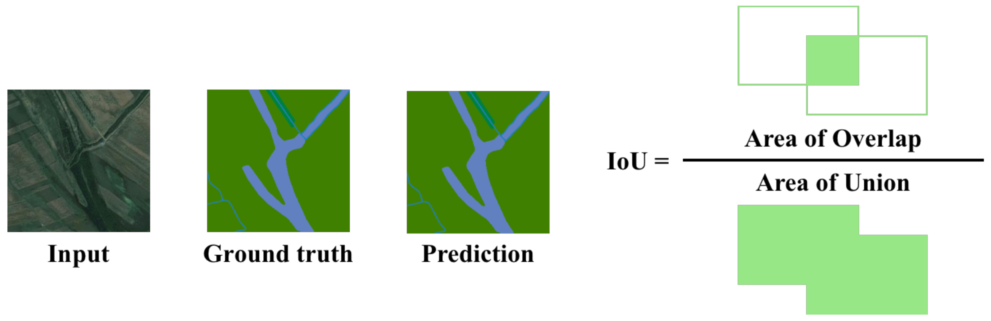
On this basis, $mIoU$ is the most commonly used performance metric in semantic segmentation to measure the degree of overlap between the predicted and actual regions, as portrayed in Figure 7.

Equation (3) provides the explicit computation process:

$$mIoU=\frac{1}{m+1}\sum _{i=0}^m\frac{p_{ii}}{{\sum }_{j=0}^m{p}_{ij}-pii}$$

(3)

Apart from calculating $mIoU$, we undertook the evaluation in terms of continuity metrics of the region based on the combination of characteristics of remote sensing tasks and evaluation metrics of the tournament where the dataset originated from. This metric is calculated as shown in Equation (4).

$$Continuity=\frac{1}{p}\sum _{i=1}^p\frac{1}{c}\sum _{j=1}^c\frac{1}{m}\sum _{k=1}^m\frac{1}{n}$$

(4)

where p represents the number of valid images, c denotes the number of valid categories in the ith graph, m denotes the number of connected domains in the jth category of ground truth in the ith graph, and n denotes the kth connected domain in the jth category of the ith graph, divided into n parts.

4.2. Rebalance the Class-Imbalance

The “hard balance” and “soft balance” are two strategies to cope with the category imbalance problem. The intuitive manifestation of category imbalance is the conspicuous gap between the amount of positive and negative samples. Automatically, the solution is to diminish the quantity difference, including expanding the positive samples and lowering the number of negative samples. Solving category imbalance by adjusting the number of categories is the idea of “hard balance”. Generally, it is always challenging to obtain additional new samples, so “hard balance” is performed by growing the number of positive samples (oversampling) or decreasing the number of negative samples (undersampling). The rudimentary effect of category imbalance is that it causes the model to focus too much on counterexamples during training, resulting in a model that is biased against counterexamples. Therefore, “soft balance” (also called rebalance in the category) ensures that the model focuses less on counterexamples by assigning smaller weights to the loss values of counterexamples; meanwhile, giving larger weights to the loss values of positive samples. Since the samples for semantic segmentation are pixels, it is hard to undertake “oversampling” and “undersampling” of the pixels in the image, so this paper chooses the “rebalance” method to address the imbalance issue.

The weights used for “rebalance” are usually negatively related to the actual number of categories. In other words, the larger the number of categories, the smaller the weights; meanwhile, the smaller the number of categories, the larger the weights. A typical median rebalance weight is calculated by taking the median $n_{median}$ of the sample size of all categories as the numerator, and the actual sample size of each category $n_i$ as the denominator, as shown in Equation (5).

$$w_i=\frac{n_{median}}{n_i},i=1,2,\cdots ,m$$

(5)

i represents the category, and m indicates the total number of categories. Equation (5) is brought into the loss function equation to obtain the weighted and rebalanced loss function, as shown in Equation (6).

$$Loss=-\frac{1}{N}\sum _{i=1}^N\sum _{c=1}^m{w}_i\widehat{y_{i,c}}ln\left(y_{i,c}\right)$$

(6)

The model performance comparison before and after rebalancing is shown in

Table 4. Comparison results of rebalancing method.

Method	Precision	Recall	mIoU	Continuity
baseline	0.870	0.859	0.864	13
rebalanced	0.917	0.883	0.901	13

, and the experimental results show that this method can effectively improve the model performance on this dataset.

4.3. Experiment Settings

This subsection presents the relevant parameter settings for the final training underlying the previous content. After analyzing the above, due to the exceptionally unbalanced distribution of categories in the dataset, this paper eventually adopted median rebalanced weights for processing, and the weights are presented in

Table 5. Corresponding weights of each class after rebalance.

Class	Weight
Buildings	0.70
Arable lands	0.04
Woodlands	0.11
Water body	0.11
Roads	5.6
Grasslands	1
Others	0.26
Unlabeled	1.90

.

The platform configuration for model training and prediction in this paper is displayed in

Table 6. Platform configuration for model training and prediction.

Item	Description
Optimizer	Adam
Initial Learning Rate	0.01
OS	Ubuntu 20.04.4 LTS
CPU	Intel i9-10900KF 3.7 GHz
GPU	RTX 3080 10 GB
Memory	32 GB

.

4.4. Training Strategies

Regarding the selection of loss functions, due to the existence of category imbalance, this study tested the softmax loss, weighted softmax loss, and Lovasz softmax loss. Each loss function has its own merits and drawbacks, which leads to the use of a single loss function for model training that may fail to help the model achieve acceptable performance. Therefore, this paper incorporated Lovasz softmax loss and softmax loss and applied this combined loss function.

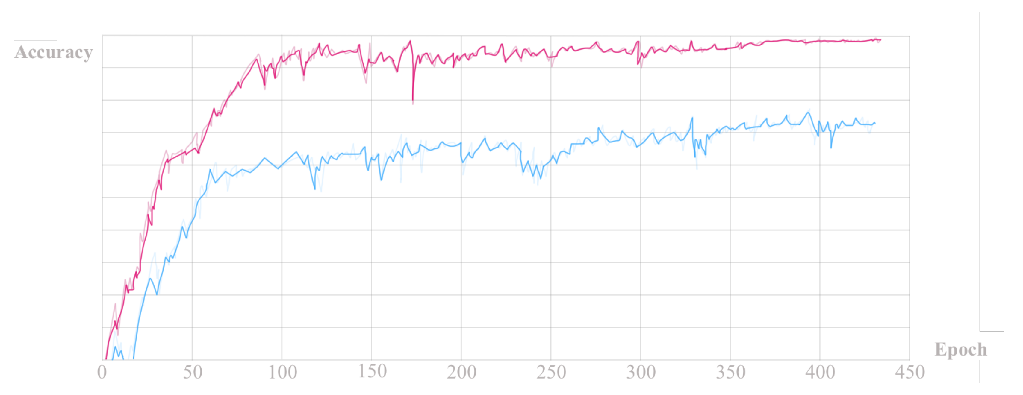
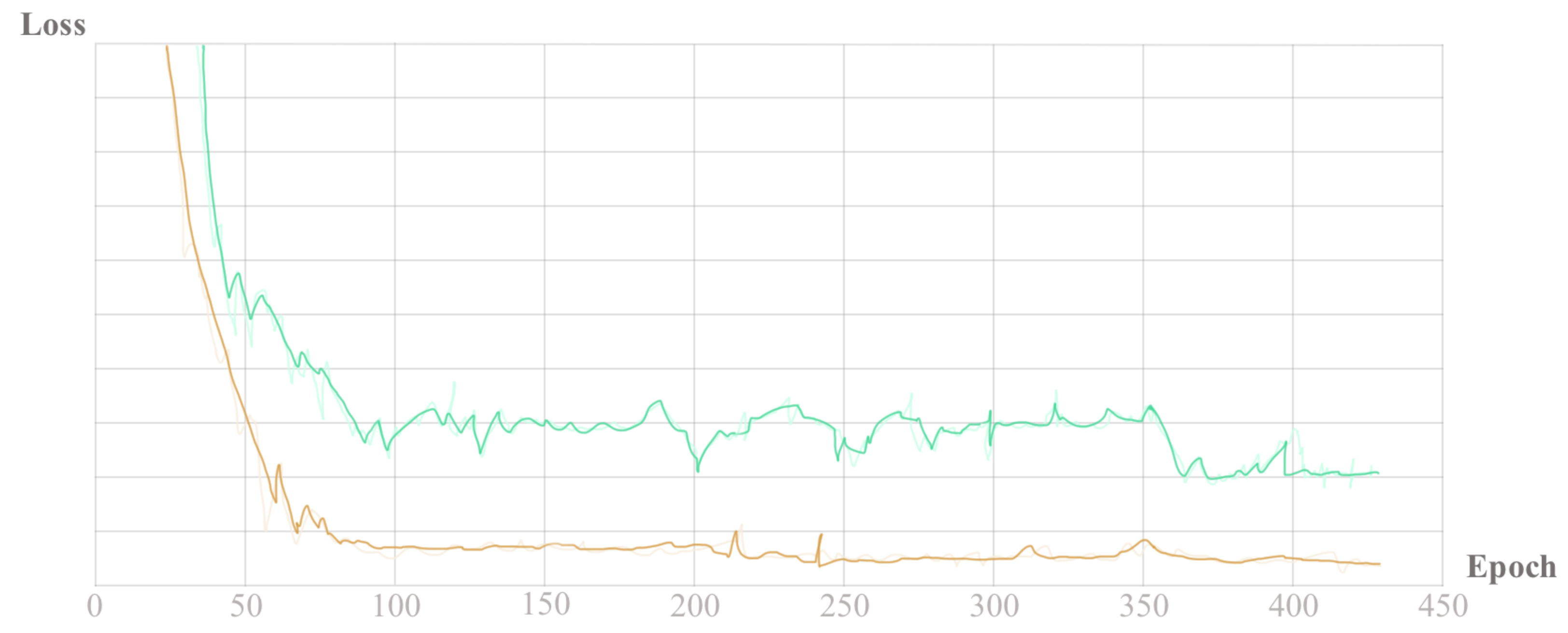
For each method model that was compared, we trained and tested on the dataset to find the most suitable method for the farming area. Figure 8 and Figure 9 display the trend in accuracy and loss during the training process.

The model parameters used in this paper are selected as the optimal parameters when the loss function converges on the training set in Figure 9.

5. Results

5.1. Validation Results

In this paper, we first tested the performance of an unoptimized model simply relying on the existing backbone and segmentation network. Afterward, we tested the model’s performance with the same training set and strategy. We found that after the global-transformer module assisted the backbone in extracting the global features, the model’s $mIoU$ improved significantly from 0.827 to 0.901. However, the continuity of the model did not improve at all. This paper thereby added the morph-module based on image morphology to the above model. The final continuity metric was dropped to 13, which was only 40.6% of the baseline, and the optimization effect was pronounced.

Table 7. Segmentation results of our model.

Model	Precision	Recall	mIoU	Continuity
UNet	0.882	0.807	0.812	29
PSPNet	0.824	0.762	0.787	53
HRNet	0.801	0.759	0.776	49
DeepLab	0.882	0.813	0.839	26
ours − baseline	0.842	0.825	0.827	32
baseline + global-transformer	0.917	0.886	0.903	29
baseline + global-transformer + morph-module	0.917	0.883	0.901	13

exhibits the performance of the proposed model on the validation set.

In this paper, it is found from comparing other networks with ours that the performance of the proposed baseline model based on the attention mechanism is still inferior to that of DeepLab. This difference is particularly pronounced in the continuity metric, 26 for DeepLab, compared to 32 for the baseline model. The reason mainly lies in the fact that the attention mechanism was merely applied to the feature extraction stage. After adding the graphical morphology processing module to the segmentation network, the continuity metric of this model was significantly improved from 32 to 13, which was significantly superior to all the comparison models. In terms of $mIoU$, DeepLab and UNet are ahead of PSPNet and HRNet with 0.839 and 0.812, respectively. Nevertheless, they are still lagging behind the final score of 0.907 for this model.

After discussing the above, we can conclude that our model has distinct advantages in both $mIoU$ and continuity. This is partly due to the optimization of the feature extraction module of the segmentation network, and partially due to the separate optimization of water bodies, roads, and other categories that are more complicated to segment and prone to multi-connected domains after segmentation. Figure 10 illustrates the strength of this model compared to the comparative model in categories with difficult segmentation and unbalanced training.

From the figure provided, the segmentation results of this model, after the enhancement of the morphology module, significantly decline in the number of connected domains of water bodies compared with other models. The segmentation effect of this model can still improve the connectivity of the segmented area compared with other models in the category of roads, where the samples are incredibly unbalanced.

Concerning the segmentation effect, this model exceeds other comparative models in terms of $mIoU$ and continuity for the weakly typed category, i.e., the category with unbalanced samples. That is primarily due to the following unique data treatments in this category.

5.2. Testing of the Model on Other Remote Sensing Datasets

The aerial images dataset released by Northwestern Polytechnical University in 2016 was employed to validate our model’s performance on other remote sensing datasets. This dataset is an open-source level 10 geospatial remote sensing dataset, containing 800 images in total—650 object images and 150 background images, with ten categories of objects: aircraft, vehicles, ships, ports, baseball fields, athletic fields, bridges, basketball courts, tennis fields, and oil tanks [28]. Since this dataset is used for the object detection task, we added the detection network after the backbone of our model, retrained it, and conducted experiments. Experimental results are exhibited in

Table 8. Validation of the applicability of the model in this paper on other remote sensing datasets.

Model	Input Size	Precision	Recall	mAP	FPS
SSD	300 × 300	83.96	80.23	87.64	33.7
	512 × 512	86.43	86.26	91.27	32.3
FSSD	300 × 300	89.76	94.37	94.85	32.9
	512 × 512	93.75	96.89	96.31	32.2
RefineDet	300 × 300	94.34	98.28	96.81	27.8
	512 × 512	94.91	98.49	96.97	25.3
EfficientDet L2	300 × 300	92.10	95.33	94.98	20.8
	512 × 512	93.24	95.98	95.14	20.2
Faster RCNN	300 × 300	82.87	78.32	90.13	25.0
	512 × 512	85.29	76.91	92.20	46.7
YOLO v3	608 × 608	94.92	98.43	96.93	52.1
YOLO v4	608 × 608	94.38	98.51	97.42	57.5
YOLO v5	608 × 608	95.98	98.57	97.51	60.3
ours	300 × 300	95.87	97.13	96.89	21.3
	512 × 512	95.91	97.89	97.62	20.4

.

5.3. Model Validation for Small-Scale Objects Detection

Since the main innovation of this paper is to improve the feature extraction ability of the backbone, we applied the backbone improved by this method to the object detection network. Meanwhile, the backbone was tested on corn and wheat ears—typical small-scale crops. The corn and wheat ears images were collected from the corn-101 variety provided by the DABEINONG Group, the scientific plantation of the West Campus of China Agricultural University, and the internet. The detection results are presented in

Table 9. Validation results of feature extraction capability for small-scale objects.

Task Category—Dataset	Model	Accuracy	mAP
classification—corn	SVM	83.18%	-
	VGGNet 19	93.92%	-
	ResNet 50	95.08%	-
	DenseNet 161	96.18%	-
	ours	96.32%	-
object detection—wheat head	YOLO v3	-	0.651
	YOLO v5	-	0.696
	SSD	-	0.583
	ours	-	0.699

.

To further demonstrate the detection results of the model, Figure 11 displays the representative detection results.

Figure 11 illustrates that our model can effectively detect wheat ears in a natural scene with a complex environment. Moreover, the model still has high accuracy when the wheat ears are in extremely high density, reflecting our model’s strong feature extraction ability.

6. Discussion

6.1. Validation of Backbone

In addition to the dilated convolution and transformer structures used in this paper, other structures are used in different CNN models to extract features, such as the block idea in ResNet and the attention module. Therefore, this section will show the comparison experiments after replacing the backbone of the model with these two modules’ representative networks: SENet and ResNet.

Table 10. Comparison results of backbone feature extraction ability.

Backbone	Precision	Recall	mIoU	Continuity
ResNet 50	0.869	0.858	0.864	14
ResNet 152	0.874	0.855	0.872	9
SENet	0.903	0.865	0.881	12
ours	0.917	0.883	0.901	13

indicates that the backbone using the combination of dilated convolution and transformer has a superior ability to extract features compared to SENet and ResNet. To be more specific, it has higher Precision and Recall scores. Hence, it can be concluded that the improved method proposed in this paper has better feature extraction capability.

6.2. Weakly Class Processing

As demonstrated in Section 3.1.1, the accuracy of the model is shallow for identifying roads and grasslands categories, resulting in a comprehensively deficient performance of the model. Therefore, in this paper, some additional work was done to train the model for these two categories:

1.

For the road category, we first extracted a binary dataset from the original training set and then performed a separate binary training; here, we operated a combination of U-Net+Dice loss training to obtain the predicted road binary results. Eventually, a straightforward judgment condition, such as the matching degree of road class on two labels, was applied to override the overall prediction outcome.

2.

The prediction results revealed that the grassland category is prone to be mispredicted as arable lands. Therefore, the separate training for grassland was conducted by extracting the two categories of arable lands and grasslands for triple classification. Afterward, the same network training as that of the main model was applied. Eventually, grassland coverage in the total prediction results only occurred between the two grassland and arable land categories.

6.3. Connectivity Metrics Optimization

The connectivity metrics are particularly prominent only for the water body and road categories, and there are two principal optimization strategies:

1.

Accuracy: To start with, we must guarantee a high classification accuracy for these two categories. The accuracy of the water body category is high enough, but the accuracy of the road category is still particularly low. Therefore, the recognition accuracy of the road category needs to be improved.

2.

Connectivity: The consideration of connectivity can start from two aspects, one is from the model, selecting or improving the model to improve the connectivity integrity of the prediction results, and the other is the post-processing step to optimize the connectivity.

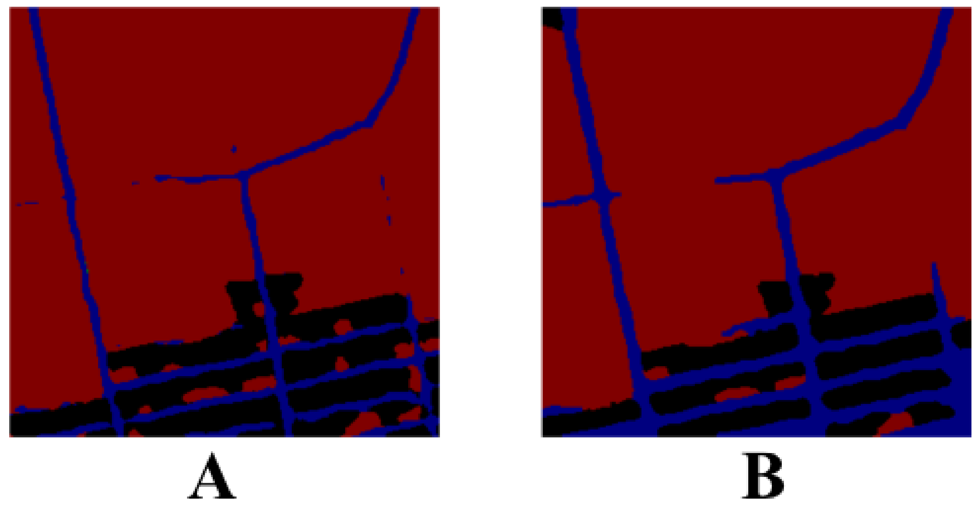
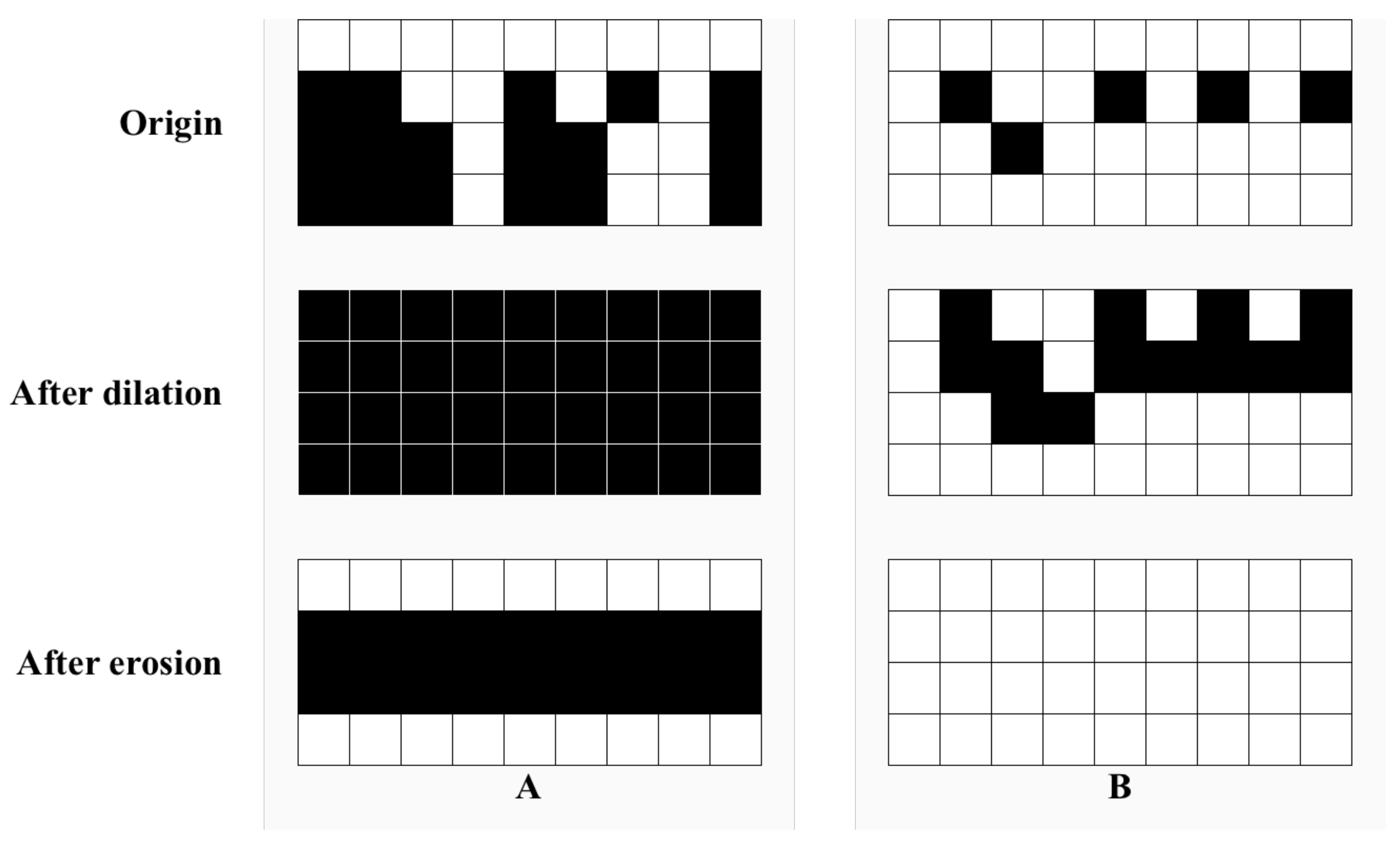
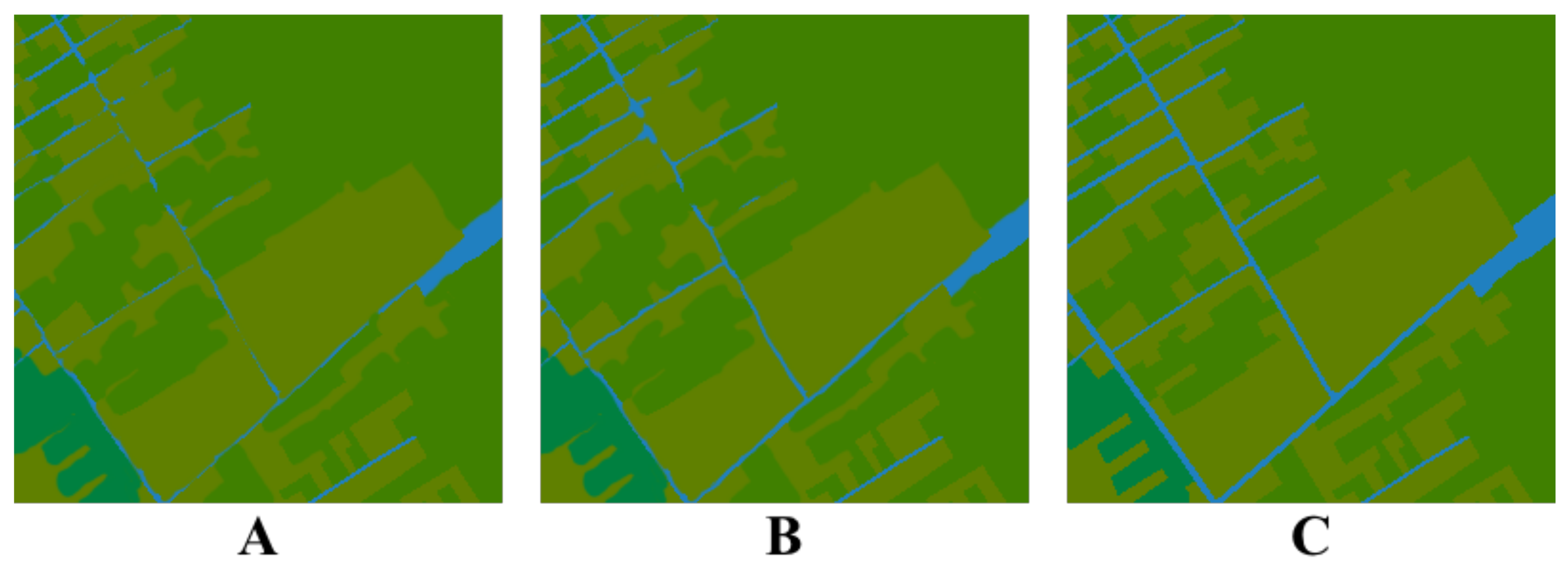
In this paper, we co-opted image morphology to improve the connectivity. The same treatment was carried out for both water bodies and roads. Firstly, the morphology was closed, and the dilation and erosion coefficients were set differently to improve the connectivity effect. Subsequently, the slight area noise was eliminated.

As illustrated in Figure 12, the road category is shown in blue, the left one is the unprocessed image, and the middle one is the morphological processed image.

6.4. Model Enhancement

6.4.1. Single Model Enhancement

Prediction enhancements for a single model typically include multi-scale prediction and flipping prediction. In order to control the prediction time, this paper only performed the prediction enhancement by flipping left and right, and flipping up and down once, i.e., flipping before prediction and then flipping back after getting the labels. Single model enhancement mainly improves prediction stability, so performing it too many times is unnecessary.

6.4.2. Model Combination Enhancement

Model combination enhancement is a model integration method, and the commonly used model integration methods include bagging, boosting, and stacking. This paper ultimately employed the hard voting method for multi-model prediction results, mainly aiming for reasoning time optimization. Multi-model enhancement mainly relies on the independence between models, so the lower the correlation between models, the better the integration effect.

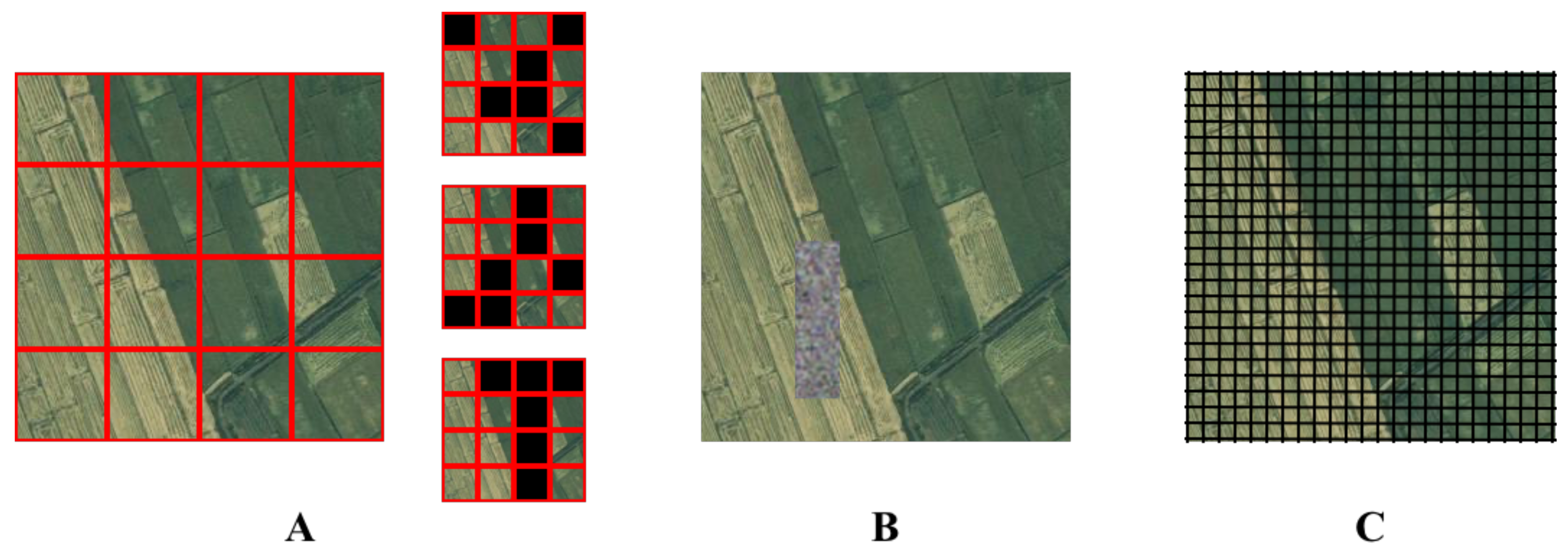
6.5. Validation of Data Enhancement Methods

In addition to the fundamental data enhancement methods, such as flipping, folding, mirroring, etc., this paper also used advanced enhancement methods requiring a certain amount of computations. These methods invoke more computations, so this section discusses whether it is reasonable to use these enhancement methods. We have done many ablation experiments, and the results are given in

Table 11. Ablation experiment result of different pre-processing methods.

Remote Erasing	Puzzle Block	Stockade Mask	Precision	Recall	mIoU	Continuity
🗸	🗸	🗸	0.917	0.883	0.901	13
🗸			0.901	0.893	0.897	15
	🗸		0.899	0.875	0.882	13
		🗸	0.913	0.883	0.904	14
			0.862	0.859	0.860	17

.

Table 11 indicates that the model’s performance decreases significantly when only utilizing the basic augmentation method, compared to the previous experimental results in this paper. Moreover, all of these enhancement methods have improved the model’s performance. Stockade Mask has the most significant effect on the model, improving by 4.9%, 3.4%, 3.7%, and 2.0% in precision, recall, $mIoU$, and continuity, respectively.

6.6. Limitation

The worst segmentation effect in this dataset is the road category, resulting in the degradation of the overall model performance. To be more precise, this category has the traits of slimness and length in the image. Although this paper has selected a separate model for the road category for training, the outcome is unsatisfactory. To optimize the segmentation effect of this category, the focus is on improving its connectivity metrics. Although the segmentation effect has been improved by morphological processing, the prerequisite—a favorable recognition rate—is required. Achieving superior segmentation results in the case of a low recognition rate is difficult. Therefore, to further improve the segmentation of these images, optimizations of the recognition rate should be considered in future work.

7. Conclusions

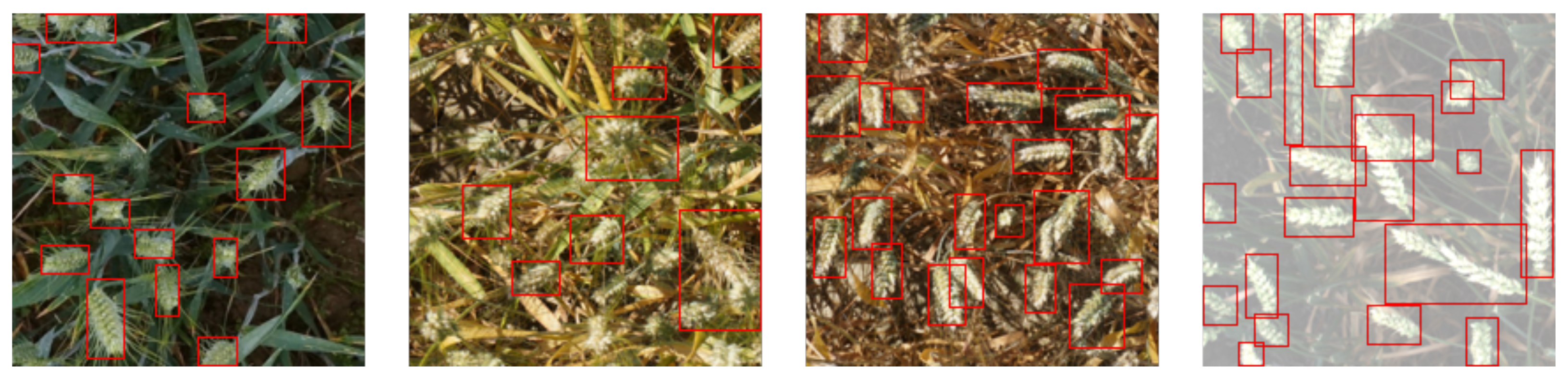
Farming areas have substantial socio-economic value in terms of farmer livelihoods, societal prosperity, and agricultural research. Detecting crops (such as wheat and corn) in farming areas permits the supervision of farming area production, and is significant for managing agricultural resources. Motivated by this practical significance, this paper proposed a global-transformer segmentation network based on the morphological correction method. The suggested model tackled the drawbacks of current image segmentation methods—their homogeneity and insufficiency in segmenting multiple objects in farming areas, as well as small-scale objects such as corn and wheat. Moreover, unlike traditional models, our model incorporated the dilated convolution technique and the transformer technique in the backbone and the branches, respectively. Because this innovation improved the feature extraction capability of the model’s backbone, the backbone enhanced by this method was applied to an object detection network on a corn and wheat ear dataset. Experimentally, our model can satisfactorily detect wheat ears in a complicated environment.

The proposed method can improve the global feature extraction ability of the model while simplifying the model structure and reducing the number of parameters, which can satisfactorily enhance the segmentation effect of small-scale objects. The morphological correction method can process the initial segmentation results, effectively minimizing the number of connected domains of narrow objects such as water bodies and roads, making the segmentation results smooth and coherent. The method finally reached 0.903 in $mIoU$ and 13 for continuity, implying that the proposed scheme is as effective as expected, and is superior to other comparison models. More precisely, the continuity has risen by 408%. These outcomes reveal that the proposed method is superior and validated on diverse datasets, demonstrating its fine generalizability. This method can provide rudimentary preparations and viable strategies for detecting crops and managing farming area resources.

As described in Section 5, the effect of morphological correction is based on the segmentation effect. Therefore, further enhancing the segmentation accuracy of remote sensing images, especially in small-scale objects, will be the future work and subsequent research interest of the authors in this paper.

References

1. Wang, L.; Anna, H.; Zhang, L.; Xiao, Y.; Wang, Y.; Xiao, Y.; Liu, J.; Ouyang, Z. Spatial and temporal changes of arable land driven by urbanization and ecological restoration in China. Chin. Geogr. Sci. 2019, 29, 809–819. [Google Scholar] [CrossRef] [Green Version]
2. Zhao, Y.; Liu, Z.; Wu, J. Grassland ecosystem services: A systematic review of research advances and future directions. Landsc. Ecol. 2020, 35, 793–814. [Google Scholar] [CrossRef]
3. Wang, W.; Yang, Y.; Li, J.; Hu, Y.; Luo, Y.; Wang, X. Woodland labeling in Chenzhou, China, via deep learning approach. Int. J. Comput. Intell. Syst. 2020, 13, 1393. [Google Scholar] [CrossRef]
4. Elagouz, M.; Abou-Shleel, S.; Belal, A.; El-Mohandes, M. Detection of land use/cover change in Egyptian Nile Delta using remote sensing. Egypt. J. Remote Sens. Space Sci. 2020, 23, 57–62. [Google Scholar] [CrossRef]
5. Mendes, W.R.; Araújo, F.M.U.; Dutta, R.; Heeren, D.M. Fuzzy control system for variable rate irrigation using remote sensing. Expert Syst. Appl. 2019, 124, 13–24. [Google Scholar] [CrossRef]
6. Ennouri, K.; Kallel, A. Remote sensing: An advanced technique for crop condition assessment. Math. Probl. Eng. 2019, 2019, 9404565. [Google Scholar] [CrossRef] [Green Version]
7. Fuentes-Pacheco, J.; Torres-Olivares, J.; Roman-Rangel, E.; Cervantes, S.; Juarez-Lopez, P.; Hermosillo-Valadez, J.; Rendón-Mancha, J.M. Fig plant segmentation from aerial images using a deep convolutional encoder-decoder network. Remote Sens. 2019, 11, 1157. [Google Scholar] [CrossRef] [Green Version]
8. Tsuichihara, S.; Akita, S.; Ike, R.; Shigeta, M.; Takemura, H.; Natori, T.; Aikawa, N.; Shindo, K.; Ide, Y.; Tejima, S. Drone and GPS sensors-based grassland management using deep-learning image segmentation. In Proceedings of the 2019 Third IEEE International Conference on Robotic Computing (IRC), Naples, Italy, 25–27 February 2019; pp. 608–611. [Google Scholar]
9. Johenneken, M.; Drak, A.; Herpers, R.; Asteroth, A. Multimodal Segmentation Neural Network to Determine the Cause of Damage to Grasslands. In Proceedings of the IEEE 2021 International Conference on Software, Telecommunications and Computer Networks (SoftCOM), Split, Hvar, Croatia, 23–25 September 2021; pp. 1–6. [Google Scholar]
10. Wang, W.; Ma, Q.; Huang, J.; Feng, Q.; Zhao, Y.; Guo, H.; Chen, B.; Li, C.; Zhang, Y. Remote Sensing Monitoring of Grasslands Based on Adaptive Feature Fusion with Multi-Source Data. Remote Sens. 2022, 14, 750. [Google Scholar] [CrossRef]
11. Iandola, F.N.; Han, S.; Moskewicz, M.W.; Ashraf, K.; Dally, W.J.; Keutzer, K. SqueezeNet: AlexNet-level accuracy with 50x fewer parameters and< 0.5 MB model size. arXiv 2016, arXiv:1602.07360. [Google Scholar]
12. Alom, M.Z.; Taha, T.M.; Yakopcic, C.; Westberg, S.; Sidike, P.; Nasrin, M.S.; Van Esesn, B.C.; Awwal, A.A.S.; Asari, V.K. The history began from alexnet: A comprehensive survey on deep learning approaches. arXiv 2018, arXiv:1803.01164. [Google Scholar]
13. Yu, W.; Yang, K.; Bai, Y.; Xiao, T.; Yao, H.; Rui, Y. Visualizing and comparing AlexNet and VGG using deconvolutional layers. In Proceedings of the 33 rd International Conference on Machine Learning, New York, NY, USA, 19–24 June 2016. [Google Scholar]
14. Sengupta, A.; Ye, Y.; Wang, R.; Liu, C.; Roy, K. Going deeper in spiking neural networks: VGG and residual architectures. Front. Neurosci. 2019, 13, 95. [Google Scholar] [CrossRef] [PubMed]
15. Targ, S.; Almeida, D.; Lyman, K. Resnet in resnet: Generalizing residual architectures. arXiv 2016, arXiv:1603.08029. [Google Scholar]
16. Bordes, A.; Bottou, L.; Gallinari, P. SGD-QN: Careful quasi-Newton stochastic gradient descent. J. Mach. Learn. Res. 2009, 10, 1737–1754. [Google Scholar]
17. Wang, P.; Chen, P.; Yuan, Y.; Liu, D.; Huang, Z.; Hou, X.; Cottrell, G. Understanding convolution for semantic segmentation. In Proceedings of the 2018 IEEE Winter Conference on Applications of Computer Vision (WACV), Lake Tahoe, NV, USA, 12–15 March 2018; pp. 1451–1460. [Google Scholar]
18. Liu, S.; Qi, L.; Qin, H.; Shi, J.; Jia, J. Path aggregation network for instance segmentation. In Proceedings of the IEEE Conference on Computer Vision and Pattern Recognition, Salt Lake City, UT, USA, 18–23 June 2018; pp. 8759–8768. [Google Scholar]
19. Kirillov, A.; He, K.; Girshick, R.; Rother, C.; Dollár, P. Panoptic segmentation. In Proceedings of the IEEE/CVF Conference on Computer Vision and Pattern Recognition, Long Beach, CA, USA, 16–17 June 2019; pp. 9404–9413. [Google Scholar]
20. Long, J.; Shelhamer, E.; Darrell, T. Fully convolutional networks for semantic segmentation. In Proceedings of the IEEE Conference on Computer Vision and Pattern Recognition, Boston, MA, USA, 7–12 June 2015; pp. 3431–3440. [Google Scholar]
21. Li, X.; Chen, H.; Qi, X.; Dou, Q.; Fu, C.W.; Heng, P.A. H-DenseUNet: Hybrid densely connected UNet for liver and tumor segmentation from CT volumes. IEEE Trans. Med. Imaging 2018, 37, 2663–2674. [Google Scholar] [CrossRef] [PubMed] [Green Version]
22. Badrinarayanan, V.; Kendall, A.; Cipolla, R. Segnet: A deep convolutional encoder-decoder architecture for image segmentation. IEEE Trans. Pattern Anal. Mach. Intell. 2017, 39, 2481–2495. [Google Scholar] [CrossRef] [PubMed]
23. Zhong, Z.; Zheng, L.; Kang, G.; Li, S.; Yang, Y. Random erasing data augmentation. In Proceedings of the AAAI Conference on Artificial Intelligence, Worcester, MA, USA, 19–23 October 2020; Volume 34, pp. 13001–13008. [Google Scholar]
24. DeVries, T.; Taylor, G.W. Improved regularization of convolutional neural networks with cutout. arXiv 2017, arXiv:1708.04552. [Google Scholar]
25. Chen, P.; Liu, S.; Zhao, H.; Jia, J. Gridmask data augmentation. arXiv 2020, arXiv:2001.04086. [Google Scholar]
26. Li, P.; Li, X.; Long, X. FenceMask: A Data augmentation approach for pre-extracted image features. arXiv 2020, arXiv:2006.07877. [Google Scholar]
27. Zhang, Y.; Liu, X.; Wa, S.; Chen, S.; Ma, Q. GANsformer: A Detection Network for Aerial Images with High Performance Combining Convolutional Network and Transformer. Remote Sens. 2022, 14, 923. [Google Scholar] [CrossRef]
28. Cheng, G.; Han, J.; Zhou, P.; Guo, L. Multi-class geospatial object detection and geographic image classification based on collection of part detectors. ISPRS J. Photogramm. Remote Sens. 2014, 98, 119–132. [Google Scholar] [CrossRef]
Figure 1. Examples of basic image preprocessing methods.
Remotesensing 14 01771 g001
Figure 2. Data pre-processing methods. (A) is Remote Erasing; (B) is Puzzle Block; (C) is Stockade Mask.
Remotesensing 14 01771 g002
Figure 3. Illustration of our model.
Remotesensing 14 01771 g003
Figure 4. The effect of dilated convolution layers with different structures on pixel sampling.
Remotesensing 14 01771 g004
Figure 5. Visualization of the effect of reducing the number of connected domains. (A) Initial segmentation result of roads; (B) Optimized segmentation result after applying morphology processes.
Remotesensing 14 01771 g005
Figure 6. Process of morphology module reduces the number of connected domains and removes noise. (A) Large noise in the segmentation; (B) Small noise in the segmentation.
Remotesensing 14 01771 g006
Figure 7. Calculation process of IoU metric.
Remotesensing 14 01771 g007
Figure 8. Training curves of accuracy against number of epochs (red: training set; blue: validation set).
Remotesensing 14 01771 g008
Figure 9. Training curves of loss against number of epochs (yellow: training set; green: validation set).
Remotesensing 14 01771 g009
Figure 10. Visualization of segmentation results. (A) our model; (B) UNet; (C) PSPNet; (D) HRNet; (E) DeepLab.
Remotesensing 14 01771 g010
Figure 11. Validation results of our model for small-scale object feature extraction capability on wheat ears dataset. Red boxes: the detected wheat ears.
Remotesensing 14 01771 g011
Figure 12. Comparison of segmentation image continuity. (A) is the segmented image without morphology module processing; (B) is the processed image; (C) is the ground truth.
Remotesensing 14 01771 g012