Abstract
Radar quantitative precipitation estimation (QPE) is one of the primary tasks of weather radars. The QPE quality was substantially improved after polarimetric upgrade of the radars. This study provides an overview of existing polarimetric methodologies for rain and snow estimation and their operational implementation. The variability of drop size distributions (DSDs) is a primary factor affecting the quality of rainfall estimation and its impact on the performance of various radar rainfall relations at S, C, and X microwave frequency bands is one of the focuses of this review. The radar rainfall estimation algorithms based on the use of specific attenuation A and specific differential phase KDP are the most efficient. Their brief description is presented and possible ways for their further optimization are discussed. Polarimetric techniques for the vertical profile of reflectivity (VPR) correction at longer distances from the radar are also summarized. Radar quantification of snow is particularly challenging and it is demonstrated that polarimetric methods for snow measurements show good promise. Finally, the article presents a summary of the latest operational radar QPE products available in the US by integration of the information from the WSR-88D radars via the Multi-Radar Multi-Sensor (MRMS) platform.
1. Introduction
Quantitative precipitation estimation (QPE) is one of the primary tasks of weather radars. It is hard to overestimate a societal impact of accurate precipitation measurements in the context of global warming with the rapidly increasing frequency of devastating flash flood events, particularly those associated with landfalling hurricanes and typhoons causing massive damage to property and infrastructure as well as human fatalities. While accurate precipitation measurements are critical for storm warnings and hydrology, they are also important for assimilation into the NWP models and optimization of their microphysical parameterization.
Traditional radar methods of rain and snow estimation were based on the use of a single radar variable, radar reflectivity factor Z. Significant progress in radar QPE was achieved during last 2–3 decades with introduction of polarimetric weather radars which are capable of complementing measurements of Z with additional radar variables such as differential reflectivity ZDR, specific differential phase KDP, and most recently, specific attenuation A. The advantages of polarimetric radar measurements for rainfall estimation were demonstrated in a number of research studies back in the nineties and early 2000s [1,2,3,4,5,6,7]. It was shown that the use of multiple radar variables helps to reduce the QPE uncertainty caused by the drop size distribution (DSD) variability whereas the utilization of a specific differential phase KDP allows to address the issues of radar miscalibration, attenuation, and partial beam blockage.
In the 2000s, the polarimetric technology and methodology for rainfall estimation matured to the point to justify their operational implementation on the nationwide weather radar networks. The US spearheaded this effort after successful completion of the Joint Polarization Experiment (JPOLE) demonstration project [8] which culminated in the polarimetric upgrade of all WSR-88D radars in 2013. Another important step was integration of the information from the WSR-88D radars using the Multi-Radar Multi-Sensor (MRMS) platform that combines the polarimetric radar data with atmospheric environment data, satellite data, and lightning and rain gauge observations to generate a suite of severe weather and QPE products [9].
A comprehensive overview of the modern polarimetric radar methods for rain and snow estimation can be found in the recent monograph of Ryzhkov and Zrnic [10] (their Chapter 10). The purpose of this review paper is to briefly summarize the QPE methodologies described in [10] and to provide an update on the recent progress in polarimetric radar QPE and its operational implementation after the monograph was published. Although we attempted to provide a summary of all relevant research around the globe, the primary focus of this review is on the last decade developments in the US. In Section 2, we describe the evolution of polarimetric methods for rainfall estimation at the distances where the radar sampling volume is below the melting layer (ML) and is primarily filled with raindrops occasionally mixed with graupel and hail. The impact of the DSD variability on the performance of various rainfall relations is discussed along with the comparative analysis of their performance in rain of different microphysical types and intensity in the S, C, and X frequency bands. The emphasis is on the most recent rainfall estimation algorithm operationally implemented on the WSR-88D network based on the combined use of specific attenuation A, KDP, and Z and its further optimization. At longer distances, where the radar samples the hydrometeors within the melting layer and above, the methods for the vertical reflectivity profile (VPR) correction are traditionally utilized. A description of the latest polarimetric VPR techniques is also presented in Section 2.
Radar measurements of snow are challenging due to tremendous variability of snow particle size distributions, their density, water content, shape, and orientation. Until recently, radar methods for estimation of snowfall rate or snow water equivalent (S or SWE) utilize multiple power-law relations between S and radar reflectivity Z. These relations exhibit roughly an order of magnitude difference in the estimates of snowfall rate for the same Z. Polarimetric methods for snow measurements have been introduced in the last few years and their description and performance results are provided and discussed in Section 3.
Section 4 contains a brief overview of the MRMS system for integration of the polarimetric radar data across the US and generation of various QPE products which are evaluated in real time with a multitude of surface rain gauges.
2. Rainfall Estimation
2.1. Polarimetric Rainfall Relations
The variability of drop size distributions is a primary source of uncertainty in the radar rainfall estimation. Because radar reflectivity Z is the 6th moment of DSD and rain rate R is approximately proportional to its 3.67th moment [10], the magnitude of Z is determined by the contribution of a few largest drops in the raindrop size spectrum whereas a bulk of smaller drops dominate rain rate. This dictated the use of multiple R(Z) relations for single-polarization radars. The choice of a particular relation depends on the type of rain (convective vs. stratiform, tropical vs. continental, etc.), season, and climate region. For example, the following five R(Z) relations are utilized on the US network of WSR-88Ds:
The choice of a particular R(Z) relation is at the discretion of a radar operator/meteorologist and there are no objective criteria for choosing an optimal one for a provided time and location.
Historically, the first polarimetric rainfall relations used a combination of Z and ZDR [11]. Utilization of ZDR, a polarimetric radar variable that depends on the median volume diameter of raindrops and is insensitive to their concentration, together with Z was expected to reduce the sensitivity of the rain rate estimate to the DSD variability. However, ZDR is even more affected by a few largest raindrops than Z. Therefore, the benefit of using the R(Z, ZDR) estimator instead of the R(Z) relation turned out to be relatively marginal. Utilization of the radar variables such as KDP and A provided better improvement because both of these variables are proportional to the DSD moments that are much closer to the 3.67th moment than Z and are immune to the radar calibration errors, attenuation in rain, and partial beam blockage.
The sensitivity of the R(Z), R(Z, ZDR), R(KDP), and R(A) estimates to the DSD variability at S, C, and X bands is illustrated in Figure 1, Figure 2 and Figure 3. Scatterplots of rain rates versus their estimates from the four optimal relations were generated using a large disdrometer dataset obtained in Oklahoma [12]. It is obvious from all three figures that the R(Z, ZDR) scatterplots are only slightly narrower than the R(Z) scatterplots and combining Z and ZDR may not result in tangible QPE improvement. Moreover, additional measurement errors of ZDR associated with its possible miscalibration and differential attenuation can make the performance of the R(Z, ZDR) algorithm even worse than the R(Z) relation. Nevertheless, certain advantages of using R(Z, ZDR) relations at S and C bands were reported in a number of studies [5,6,13,14,15,16,17,18,19,20]. Many of these relations can be found in Ryzhkov and Zrnic [10] (their table 10.3). It is not instrumental to utilize a combination of Z and ZDR for rainfall estimation at X band because their biases caused by attenuation/differential attenuation are too large and difficult to account for.
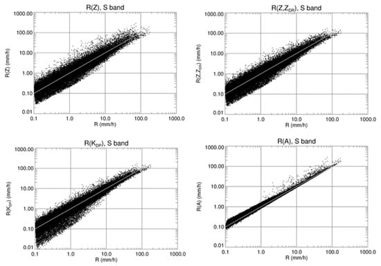
Figure 1.
Scatterplots of rain rates versus their estimates from relations , , , and optimized for Oklahoma DSD dataset at S band (λ = 11.0 cm) and T = 20 °C. Z and ZDR are in a linear scale.
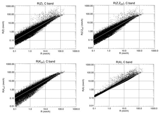
Figure 2.
Scatterplots of rain rates versus their estimates from relations , , , and optimized for Oklahoma DSD dataset at C band (λ = 5.3 cm) and T = 20 °C. Z and ZDR are in a linear scale.
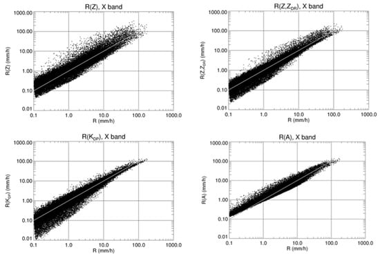
Figure 3.
Scatterplots of rain rates versus their estimates from relations , , , and optimized for Oklahoma DSD dataset at X band (λ = 3.2 cm) and T = 20 °C. Z and ZDR are in a linear scale.
The R(KDP) scatterplots in Figure 1, Figure 2 and Figure 3 exhibit obvious benefit of the R(KDP) relations for estimation of moderate-to-heavy rain at all three microwave frequency bands. A simple rule can be formulated as follows: the R(KDP) relation is advantageous for measuring rain rate R if the value of R expressed in mm/h exceeds the value of radar wavelength λ in cm (e.g., [21]). This means that the R(KDP) estimator is efficient for R > 10–11 mm/h at S band, for R > 5–6 mm/h at C band, and for R > 3 mm/h at X band. Utilization of R(KDP) at lower rain rates is generally counterproductive because the R(KDP) estimator becomes very sensitive to the DSD variability as can be seen from Figure 1, Figure 2 and Figure 3 and the estimates of KDP itself become very noisy. Such a noisiness, however, can be reduced by averaging of KDP over a large spatial/temporal domain and the R(KDP) algorithm remains efficient even in light rain for areal rainfall estimation [22] or monthly rain accumulation [23].
A more quantitative assessment of relative performance of different rainfall relations can be obtained using Figure 4 where the dependencies of the fractional mean absolute error (fMAE) on rain rate for the R(Z), R(Z, ZDR), R(KDP), and R(A) relations optimized for the Oklahoma DSDs at S, C, and X bands are shown. The advantages of all three polarimetric relations compared with the R(Z) relation are obvious in a wide range of rain intensities at all three microwave bands. The R(A) relation (which will be discussed in more detail in the next Section 2.2) is an apparent winner at low-to-moderate rain rates. The R(A) advantage is particularly impressive at S band where the fMAE caused by the variability of DSD is less than 10% in a wide range of rain intensities. For higher rain rates exceeding 10 mm/h, fMAE tends to increase at C and X bands for all relations except R(KDP) that is least sensitive to the effect of the resonance scattering on large raindrops which is primarily responsible for such an increase. Therefore, the KDP-based relation is an obvious choice for heavy rain at C and X band.
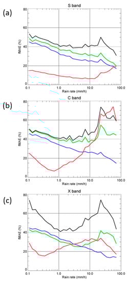
Figure 4.
Dependencies of the fractional mean absolute error (fMAE) on rain rate for the R(Z) (black curves), R(Z, ZDR) (green curves), R(KDP) (blue curves), and R(A) (red curves) relations optimized for the Oklahoma DSDs at S, C, and X bands panels (a), (b), and (c), respectively.
Because KDP is proportional to the radial derivative of differential phase ΦDP, it is immune to radar miscalibration, attenuation, partial beam blockage, and presence of water or snow on the surface of a radome. The immunity of KDP to attenuation makes it particularly beneficial for rainfall measurements at shorter wavelengths. The R(KDP) relation is commonly used if rain is mixed with hail as was originally recommended by Balakrishnan and Zrnic [24]. Until recently, it was believed that hail does not contribute much to KDP. This is not the case for melting graupel and water-coated hail of small size and high concentration. Moreover, small, and wet graupel/hail can produce anomalously high KDP well-exceeding typical values of KDP in rain. For example, Kumjian et al. [25] measured KDP as high as 17 deg/km at S band in a storm producing large accumulations of small hail. If such a value of KDP is converted to rain rate using a standard S-band relation R(KDP) = 44.0|KDP|0.822, it would yield an unrealistic rain rate of 452 mm/h. In order to mitigate such an obvious overestimation, the R(KDP) with a smaller multiplier is recommended if the cross-correlation coefficient ρhv drops below a certain level (0.97) in areas of high Z indicating the presence of hail [26], see Section 4. The KDP-based algorithms for rainfall estimation were used in a large number of studies and operational applications (e.g., [1,2,3,5,6,7,13,14,15,27,28,29,30,31,32,33,34,35,36,37,38,39,40,41]). A long list of various R(KDP) relations can be found in [10] (their Table 10.3).
2.2. Attenuation-Based Rainfall Retrievals
A game-changer during the last decade was the introduction of the rainfall estimation methodology based on specific attenuation A [20,26,39,41,42,43,44,45,46,47,48]. Because this methodology is relatively new, herein we provide its description in more detail compared with other rainfall estimation techniques. A radial profile of A can be retrieved from the radial profile of attenuated Za and two-way path integrated attenuation PIA along the propagation path (r1,r2) in rain as [42]
where
In Equations (2)–(5), the factor b is a constant parameter (usually between 0.6 and 0.9 at microwave frequencies). The value of PIA cannot be estimated with a single-polarization radar but can be computed from the total span of a differential phase ΔΦDP measured by a dual-polarization radar:
where α is equal to the average ratio of A and KDP along the propagation path.
It follows from Figure 1, Figure 2, Figure 3 and Figure 4 that the R(A) estimate is much less affected by the DSD variability because the R(A) scatterplots are significantly narrower than the ones for the R(Z), R(Z, ZDR), and R(KDP) relations, particularly at S band. Therefore, the R(A) algorithm has a chance to work best of all these relations at S band where attenuation in rain is lowest. At first glance, this seems counterintuitive. However, even small path integrated attenuation PIA can be estimated reliably because of its strong correlation with ΔΦDP according to Equation (6). The R(A) relation is almost linear at S band:
where λ = 11.0 cm and T = 20 °C ([42]). It deviates from linearity at C and X bands because of the more pronounced effects of resonance scattering on raindrops at shorter wavelengths. As a result, the effectiveness of utilizing specific attenuation at C and X bands for rainfall estimation is lower than at S band. It is evident from Figure 2, Figure 3 and Figure 4 that the R(A) relation has apparent advantages for lower rain rates whereas the R(KDP) relation seems to be optimal for heavy rain. One of the advantages of the R(A) estimates compared with R(KDP) is its better radial resolution which is similar to the one of Z and R(Z).
The radar retrieval formulas used for plotting scattergrams in Figure 1, Figure 2 and Figure 3 are optimized for a disdrometer dataset obtained in Oklahoma. The parameters of radar rainfall relations vary depending on rain type, therefore such relations should be adjusted using DSD data collected in a particular climate or geographical area. Microphysical characteristics of rain may vary in a wide range even in a particular geographical region such as Oklahoma. Different types of rain can be distinguished using the average dependencies of ZDR on Z. Figure 5 shows Z–ZDR dependencies corresponding to different percentiles of ZDR for a given Z in rain simulated from 47114 DSDs measured in Oklahoma. The simulations are for S band at T = 20 °C. A tropical rain, a bulk of which is generated via a “warm rain” process below the melting layer, is commonly characterized by high concentration of small- and medium-size drops with a relative deficit of large drops which results in a lower value of ZDR at a given Z as in the 0–20% range of ZDR between two lowest curves in Figure 5. A continental rain, mostly originated from melting ice, is usually dominated by large raindrops with a lower concentration of small drops as opposed to the tropical rain and is characterized by higher values of ZDR for a given Z. The two families of DSDs belonging to the 0–20% and 80–100% ranges can be designated as “very tropical” and “very continental” rain. In Figure 6, the log(R) vs. A scatterplots corresponding to the very tropical rain at S, C, and X bands are marked by red symbols, whereas the very continental scatterplots are presented in blue symbols. It is evident that the clusters associated with these two rain types almost coincide at S band and become more separated at C and X bands. The R(A) relations are especially beneficial for lower rain rates and for tropical rain of any intensity (red clusters). At C and X bands, the separation between red and blue clusters identifies that different R(A) relations must be utilized for tropical and continental rain. For a given rain rate, the value of A is larger for a continental rain which means that the multiplier in the R(A) relation should be lower for a continental rain. It can be shown that a similar rule is applied for the R(KDP) and R(Z) relations.
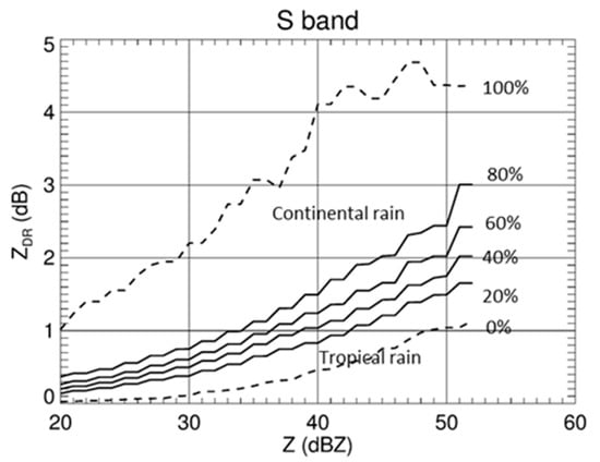
Figure 5.
Lines of different percentiles of the ZDR distributions for a given Z obtained from the Oklahoma DSD measurements.
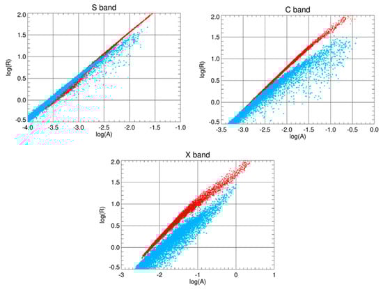
Figure 6.
Scatterplots of log(R) vs. log(A) at S, C, and X bands for “very tropical” rain (red dots) and “very continental” rain (blue dots). Specific attenuation is computed for the temperature 20 °C.
Specific attenuation is a strong function of radar wavelength λ and temperature T; therefore, the parameters of the power-law R(A) relation are also wavelength- and temperature-dependent. At S band, this, however, does not preclude the use of a single R(A) relation specified by Equation (7). As is shown in [10], the value of A estimated from Equation (2) is approximately proportional to the magnitude of the parameter α which is proportional to A and depends on λ and T in a similar manner. This leads to almost complete cancellation of both dependencies in the final estimate of R which allows using a single R(A) relation provided by Equation (7). Note, that such cancellation is incomplete at C and X bands and a single R(A) relation is not as accurate as at S band.
A very important advantage of the KDP- and A-based QPE algorithms is their immunity to the radar miscalibration, attenuation in rain, partial beam blockage, and impact of a wet radome. The immunity to partial beam blockage is illustrated in Figure 7 where the fields of 6-h rain total computed from R(Z) and R(A) are displayed. Large negative bias in the rain totals retrieved from R(Z) associated with partial beam blockage caused by trees near the radar is completely eliminated in the rain field estimated from R(A).
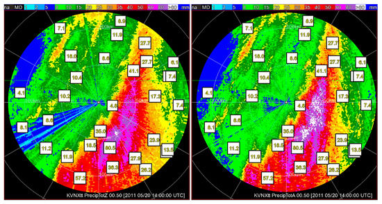
Figure 7.
Maps of 6-h rain total obtained from the KVNX WSR-88D radar on 20 May 2011 (0800–1400 UTC) using R(Z) and R(A) algorithms. Gauge accumulations (mm) are displayed in white squares.
All discussed radar rainfall relations have advantages and disadvantages at different rain rates and radar wavelengths. Hence, it is beneficial to use composite algorithms by combining various relations. The operational polarimetric rainfall estimation algorithm currently implemented on the WSR-88D radar network in the US uses a combination of the R(Z), R(A), and R(KDP) relations [26,46,47]. The R(KDP) relations are used in areas of high Z where rain may be mixed with hail and the R(A) relation is utilized otherwise. The QPE algorithm resorts to various R(Z) relations if the radar sample is within the melting layer or above or if the total span of differential phase ΔΦDP in rain is too small or beam blockage is severe. The details of the operational WSR-88D QPE algorithm (labeled Q3DP) are in [26] and Section 4 of this review.
The Q3DP algorithm became operational in October 2020 and has demonstrated very good performance so far, particularly in heavy rain associated with flash floods. Figure 8 illustrates its performance for the most significant flash flood events of the 2021 warm season in the US. One of them occurred in Tennessee on August 21 and resulted in 27 fatalities and another one was associated with Hurricane Ida during the period from August 30 to September 2 with a death toll of 67 people. The Hurricane Ida had its landfall in Louisiana and transformed from a tropical depression to a post-tropical cyclone that rolled into the US northeast two days later. Color-coded maps in the upper images in Figure 8 show 24-h radar-estimated rain totals and the circles, their comparison with rain gauges. The size of the circle is proportional to the rain amount whereas different shades of red and blue indicate various levels of radar underestimation and overestimation, respectively. White or pale colors indicate either the absence of bias or a small bias. Indeed, the scatterplots of 24-h totals versus their radar estimates shown in the bottom panels indicate very good performance in all three cases with the average bias below 10% and the correlation coefficient well-above 0.9.
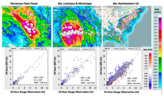
Figure 8.
(Top panels) The maps of 24-h rain total estimated using Q3DP rainfall algorithm in Tennessee during the period ending at 1200 UTC on 21 August 2021, in Louisiana during the period ending at 1200 UTC on 30 August 2021, and US northeast during the period ending at 1100 UTC on 2 September 2021. Colored dots represent CoCoRaHS gauge sites. The size of the dots represents gauge observed amounts and the color represents the gauge/QPE (G/R) bias ratios. (Bottom panels) Scatterplots of radar 24-h rain totals versus their gauge estimates. The statistic scores in the scatterplots are the bias ratio (R/G), mean absolute error (MAE), and correlation coefficient (CC).
2.3. Further Optimization of the R(A) and R(KDP) Relations
Although the polarimetric rainfall estimators R(A) and R(KDP) have undeniable advantages compared with the old Z-based methods, they may require further optimization. It was mentioned before that the R(A) relation is practically insensitive to the DSD variability (at least at S band) but the estimate of A from Equations (2)–(6) depends on DSD because the factor α is a strong function of ZDR (Figure 9). Such a dependence of α on ZDR at S band and temperature 20 °C can be approximated by equation:
where ZDR > 0.2–0.3 dB. In Equation (8), ZDR is expressed in dB. In the existing R(A) algorithm, the parameter α is optimized on the scan-to-scan basis and determined from the slope of the ZDR(Z) dependence as described in [10,26,46]. The use of a single factor α for a whole radar coverage area generally leads to some underestimation of light rain and occasional overestimation of heavy rain. This is attributed to the fact that light rain is commonly characterized by larger α whereas significantly lower α might be more typical for heavier rain often associated with deep convection, and the use of a single “net” α (or <α>) for both rain types produces such biases (see Figure 9).
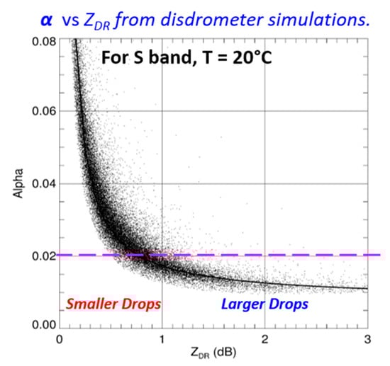
Figure 9.
The scatterplot of α versus ZDR simulated from the Oklahoma disdrometer data at λ = 11.0 cm and T = 20 °C. Black curve represents the α(ZDR) dependence specified by Equation (8).
There are a couple of possible approaches to address this issue and to take into the account an azimuthal dependence of <α>. One of them is proposed in [49] using variational principles. According to [49], the state vector X consists of the “true” values of Z and ZDR (not biased by attenuation/differential attenuation) along the radial in rain and the observation vector Y is composed of the radial profiles of the measured (attenuated) values of Z(Z(m)) and ZDR(ZDR(m)) and total differential phase ΦDP(m). The “forward operator” includes analytical relations for computing simulated KDP(s), A(s), specific differential attenuation ADP(s), and simulated differential phase ΦDP(s) from the “true” values of Z and ZDR. The components of the state vector are retrieved using the variational routine to match the simulated and measured vectors Y. After the “true” values of Z and ZDR are determined, the corresponding values of A and KDP along each ray are computed using the forward operator, and the net <α> for a provided azimuth is estimated as the ratio ΣA(i)/ΣKDP(i) where summation is performed along the propagation path in rain. Such a routine is computationally expensive, requires well-calibrated values of the measured Z(m) and ZDR(m) and its operational utilization must be demonstrated.
A possible alternative methodology implies the use of the radial profile of α(ZDR) for estimation of <α> separately for each azimuth. The “net alpha” for a provided radial of data and propagation path in rain (r1,r2) is a ratio:
Assuming A = aZb, Equation (9) can be rewritten as:
where Z is the “true” reflectivity not biased by attenuation. The net α can be also estimated using a different formula by using the KDP = cZd relation instead of the A(Z) relation.
Following [50], KDP can be expanded as:
which after substituting into Equation (11) yields:
The values of Z and ZDR in Equations (10) and (13) should be first corrected for attenuation/differential attenuation.
Azimuthal profiles of <α> estimated using Relations (10) and (13) for the case of a mesoscale convective system are presented in Figure 10 (upper right panel) using black and red dots respectively. It is obvious that Relations (10) and (13) provide very similar results. In the middle and bottom right panels, the azimuthal dependencies of Z and ZDR averaged over the whole propagation path in rain are displayed. As expected, the azimuthal dependence of <α> exhibits strong anti-correlation with averaged ZDR and the absence of correlation with averaged Z. The lowest value of <α> is observed in the azimuthal direction along the squall line in the NE sector.
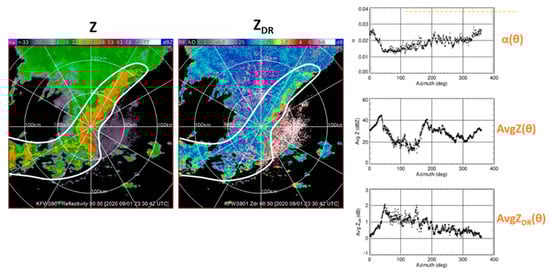
Figure 10.
PPIs of Z and ZDR measured by the KFWS WSR-88D radar on 9 January 2020 at 23:30:42 UTC (left panels). Corresponding azimuthal dependencies of the retrieved <α> and radially averaged Z and ZDR (right panels).
This routine for <α> optimization, if proven efficient, can replace the existing rather cumbersome “ZDR slope” methodology that does not allow capturing the azimuthal variability of <α>. Note that the value of <α> obtained using this technique can be used for polarimetric attenuation correction of Z that utilizes the relation ΔZ = <α> ΦDP. Most of the existing attenuation correction techniques assume a fixed value of <α> whereas the actual value of <α> can vary quite significantly with time and azimuth as Figure 10 indicates. The value of <α> obtained from Equations (10) and (13) may also be utilized for optimization of the R(KDP) relations because the parameters of these relations generally depend on DSDs and rain type. The multiplier a1 in the power-law relation should be higher for tropical rain characterized by larger <α> and lower for continental rain with smaller <α>. It can be shown that the value of a1 is equal to 35.8, 50.1, and 62.7 for b1 = 0.82 for <α> = 0.015, 0.030, and 0.050 dB/deg respectively. Such tuning of the R(KDP) relations based on the value of <α> is strongly recommended.
2.4. Polarimetric VPR
Once the radar beam intercepts the melting layer (ML) and snow/ice aloft, the relation between reflectivity (and other variables) and rain rate at the surface becomes complicated. Because Z in the ML is usually higher than in rain near the surface, the R(Z) relation valid in pure rain inevitably overestimates the surface rain rate at the distances where the radar samples ML. At longer distances where the radar resolution volume is in ice/snow above the ML, underestimation takes place. Various methods have been developed to address the melting layer problem (e.g., [51,52,53,54]). Common to these is the estimation of a vertical profile of reflectivity (VPR) and its use to retrieve rain rate near the ground. One of the ways to obtain the VPR is to scan the storm, reconstruct its structure near the radar, and extrapolate its effect to long range assuming horizontal homogeneity [53,55]. Such volume-scan VPR corrections are often part of operational algorithms for QPE. Andrieu and Creutin [56] and Andrieu et al. [57] added sophistication by applying discrete inverse theory based on hourly averaged VPRs at two elevation angles (1° and 3°). Local VPRs correction over small areas (20 km in range and 20° in azimuth) using an inverse filtering of the beam effects was proposed by Vignal et al. [58] and proven to be better in Switzerland [59] and US [60] than “global” corrections.
The concept of an “apparent” VPR or AVPR was introduced by Zhang and Qi [61] and Qi et al. [62]. The VPR correction is performed in the “bright band affected area” (BBA) within the stratiform part of the storm that is identified using radar reflectivity Z and cross-correlation coefficient ρhv. The average radial profile of Z at the lowest antenna tilt is determined within BBA and subtracted from the radial profiles of Z at each particular azimuth. Then the standard R(Z) relation is applied to estimate rain rate. Therefore, it is expected that the radial dependency of Z is entirely determined by the vertical profile of Z through the ML and the vertical structure of a storm is horizontally uniform within BBA. This methodology assumes that the BBA is relatively homogeneous azimuthally and is called “tilt-VPR”. Such an assumption can fail in the presence of frontal boundaries with large variations in the ML height which usually happens during cold season with lower ML. Hanft and Zhang [63] suggested the so-called dpVPR methodology to derive azimuthally dependent VPRs which results in the overall improvement of the VPR correction as illustrated in Figure 11. In the absence of the VPR correction, the 24-h radar derived rain totals are greatly overestimated (blue circles in Figure 11c,f). The positive QPE bias is dramatically reduced with tilt-VPR correction applied (Figure 11a,d) and the QPE results are further improved after the dpVPR correction scheme is utilized (Figure 11b,e). Note that, in addition to reducing the artificial enhancement of Z and R(Z) in BBA, the dpVPR algorithm also reduces the negative bias in R(Z) at longer distances from the radar where the radar beam is above the ML.
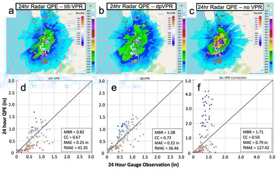
Figure 11.
Twenty-four h radar QPEs from the KRTX WSR-88D radar ending at 15:00 UTC 07 February 2017 with (a) tilt-VPR, (b) dpVPR, and (c) no VPR correction and the corresponding scatter plots vs. CoCoRaHS gauges (panels (d–f), respectively). The Z = 210 R1.46 relation is used.
An alternative methodology for polarimetric VPR (PVPR) implies determination of the heights of the ML top and bottom over large areas using the recent melting layer detection algorithm (MLDA) described in [64]. According to this methodology, a multitude of the model radial profiles of Z and ρhv at lowest antenna tilts for different heights and “strengths” of the ML are simulated and stored in lookup tables. The “strength” of the ML characterizes both its thickness and the depth of the corresponding ρhv minimum that is usually well-correlated with the Z enhancement in the ML. The simulation routine explicitly takes into account radar beam broadening that has a strong impact on the ML signature at lower antenna elevations and large distances from the radar. Then an appropriate model profile of Z at every azimuth and elevation is determined by finding the best match between the model and observed profile of ρhv. Because all simulated model profiles of Z and ρhv are labeled by the intrinsic height and strength of the ML, such a matching routine allows for estimating the parameters of the ML such as the heights of its top and bottom. In addition, a model radial profile of Z associated with these parameters of the ML is identified and subtracted from the measured radial profile of Z at a particular azimuth. The difference between the PVPR and dpVPR routines is that PVPR is essentially coupled with the MLDA and uses the model radial profiles of Z whereas dpVPR is based on the piecewise linear approximation of the measured average radial profile of Z in a narrow azimuthal interval without quantification of the ML height and depth. Both VPR techniques have the same deficiency, an assumption of radial uniformity of Z and corresponding rain rate within the range interval affected by the “bright band contamination”. The tilt-VPR and dpVPR have been validated for a significant number of rain events [61,62,63] while massive validation of PVPR is in order. The performance of the PVPR algorithm is illustrated in Figure 12 and Figure 13 for the rain event with a low ML that is very well-identified in the QVPs of Z, ZDR, ρhv, and KDP (Figure 12). The maps of hourly rain total retrieved from R(Z) in the area affected by ML before and after PVPR correction of Z measured by the KLSX WSR-88D radar are shown in Figure 13. Artificial enhancement of the estimated rain accumulation due to the increase in radar reflectivity in the ML clearly visible in the left panel is completely eliminated after PVPR is utilized (right panel).
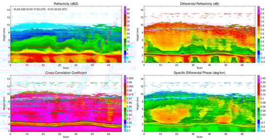
Figure 12.
Range-defined quasi-vertical profiles (RD-QVP) of Z, ZDR, KDP, and ρhv measured by the KLSX WSR-88D radar on 30 January 2021 for the period of 7 h starting on 1700 UTC.
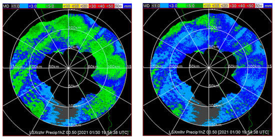
Figure 13.
Maps of hourly rain total retrieved from R(Z) in the area affected by ML before and after PVPR correction of Z measured by the KLSX WSR-88D radar during the period from 18 to 19 UTC on 30 January 2021.
Concluding this section, we must mention recent studies where artificial intelligence (AI)/machine learning (ML) algorithms were used for polarimetric QPE. This is a rapidly growing area of research stimulated by accumulation of large datasets of polarimetric radar variables combined with surface rainfall measurements and facilitated by the availability of abundant modern computer resources. A detailed analysis of the AI/ML polarimetric QPE algorithms is beyond the scope of this review and we cited recent articles by Zhang et al. [65], Shin et al. [66], and Wolfensberger et al. [67] as examples for an interested reader.
3. Polarimetric Measurements of Snow
3.1. Historical Overview
Radar snow measurements present an enormous challenge due to immense variability of snow particle size distributions (PSDs), density, shapes, orientations, crystal habits, and terminal velocities. Historically, radar reflectivity factor at horizontal polarization Z was used to estimate snow water equivalent rates S in the form of numerous power-law relations (e.g., [68,69,70,71,72,73,74,75]). The majority of these relations assume that Z is proportional to S2. Radar reflectivity is very close to the 4th PSD moment for low-density snow (e.g., aggregates) due to the inverse dependence of snow density on the snowflake size whereas S is proportional to significantly lower the order moment of PSD (2.1–2.2) [10]. This is one of the primary problems with existing S(Z) relations. The accuracy of S(Z) estimates is altitude dependent. At longer distances from the radar where the radar beam is much higher, the performance degrades due to the significant changes in Z with height, especially in aggregated snow. Despite these deficiencies, the conventional radar algorithms still utilize the standard S(Z) relations, which exhibit roughly an order of magnitude difference in the estimates of snowfall rate for the same reflectivity factor. This traditional approach is based on the usage of a multitude of climatological S(Z) relations optimized for different snow types and geographical areas. For example, the US National Weather Service (NWS) operationally uses several S(Z) relations for radar snow QPE (depending on the geographical region) as presented in Table 1 and it has not yet capitalized on the polarimetric capability of the WSR-88D radars.

Table 1.
Summary of Z(S) relations for dry snow listed in the literature and utilized by the WSR-88D network in the United States.
Various alternatives to a Z-based approach for snow QPE were recently explored through the designated field campaigns. The GPM cold-season Precipitation Experiment (GCPEx, [81]), conducted by the National Aeronautics and Space Administration (NASA, Washington, DC, USA) and Environment Canada in Ontario, Canada, was one of such campaigns with a goal to investigate the utility of the multi-frequency (active and passive) microwave sensors for better classification and quantification of snow. Huang et al. [82] utilized a dual-wavelength ratio (DWR) of reflectivities at Ku and Ka bands available from the GCPEx data to develop the S(Z) relation parametrized by DWR. The difference between Zs at Ku and Ka bands increases with the characteristic size of snowflakes and the use of a multiplier in the S(Z) relations depending on DWR, helps to reduce the PSD-related uncertainty in the radar snow estimates.
Another campaign that significantly expands our knowledge of the snow microphysics was Biogenic Aerosols—Effects on Clouds and Climate (BAECC) 2014. Von Lerber et al. [80] utilized the snow data from BAECC to investigate the connection between the snow properties and radar observations using a video disdrometer and derived event-based power-law mass-size relations for ice/snow along with the corresponding S(Z) relations. They linked the changes in the S(Z) relation’s exponent to the variations in the mass-size relation’s exponent. The multiplier of the S(Z) relation is determined by the prefactors of the mass-size and velocity-size relations and by the intercept parameter N0 of the particle size distribution. The changes in the S(Z) multiplier for a given N0 are also associated with the changes in a liquid water path, a proxy for the degree of riming. In another study which partially used BAECC data in conjunction with the data from the University of Helsinki Hyytiälä station, Tiira and Moisseev [83] developed the unsupervised method for classification of vertical profiles of polarimetric radar variables using k-means clustering. They showed that the profiles of radar variables can be grouped into 16 snow classes which capture the most important snow growth and ice cloud processes. This can be used for the development of the snow class-based S(Z) relations that capture the variability of snow PSD, density, and fall velocity.
3.2. Radar Polarimetric Relations for Snow Estimation
Radar polarimetry opens new horizons for snow habit classification and quantification (e.g., [83]). Since the advance of polarimetry, only a handful of studies have explored polarimetric quantitative snow retrievals, mostly focused on ice water content (IWC) quantification. Vivekanandan et al. [84] and Lu et al. [85] utilized a specific differential phase KDP for estimation of IWC. Aydin and Tang [86] investigated possible methods for IWC retrievals in the clouds composed of pristine ice crystals using the combination of differential reflectivity ZDR and KDP. Ryzhkov et al. [87,88] and Ryzhkov and Zrnic [10] used a combination of KDP and ZDR or KDP alone to quantify IWC of pristine or lightly-to-moderately aggregated ice. Using the instrumented aircraft, Nguyen et al. [89] derived the empirical IWC(KDP) and IWC(KDP, ZDR) relations from the airborne X-band polarimetric radar measurements and in situ microphysical probes. These empirical relations are very similar to the theoretical ones derived in [88]. Bukovčić et al. [90] introduced the first polarimetric algorithm (based on the KDP and Z) for estimation of the extinction coefficient and visibility in snow which are traditionally linked to the snowfall rates (e.g., [91,92,93,94,95,96,97]). The algorithm, tested with S-band WSR-88D radar data, showed a good potential for quantification of extinction and visibility in snow.
Hassan et al. [98] proposed one of the first polarimetric relations for snowfall rate estimation using ZDR and Z at C band. They showed that the addition of ZDR to Z produces comparable results to standard S(Z) relations. Much more success in polarimetric snow QPE can be achieved if Z is combined with specific differential phase KDP. A theoretical S(KDP, Z) relation in a form of a bi-variate power-law was derived by Bukovčić et al. [99] assuming an exponential PSD, , and Rayleigh approximation:
where λ is the radar wavelength in mm, and Z is in mm6m−3. It is also assumed that the snow density ρs and terminal velocity of snowflakes vs. are related to the particle equivolume diameter D as:
and:
where in Equation (14), Fo and Fs are the factors characterizing orientation and shape of snowflakes and parameters as and bs are the functions of δs whereas cs is a function of αs, δs, and the density of air ρa (or atmospheric pressure). The factor Fo is determined by the width of the canting angle distribution σs and the factor Fs is a function of the aspect ratio a/b of snowflakes specified in [10,99], see Figure 14. It can be shown that the theoretical Relation (14) is simplified as:
where λ = 11.0 cm, a/b = 0.65, σs = 0°, and αs = 0.178 (as in [100]).
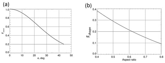
Figure 14.
(a) Orientation factor Fo as a function of the width the of canting angle distribution σ; (b) shape factor Fs as a function of the particle aspect ratio.
Relations (14) and (17) are derived for an exponential size distribution. A generalized empirical S(KDP, Z) relation is derived from the extensive Oklahoma snow 2DVD measurements of PSDs and terminal velocities assuming wide ranges of particle aspect ratios (0.5–0.8) and the canting angle distribution width σ (0–40°) [99]. It has a form:
which is very close to the theoretical Relation (17). For practical purposes, an alternative S(KDP, Z) relation can be used that explicitly takes into account the shape and orientation factors as well as air density (or atmospheric pressure p):
In Equation (19), p0 = 1013 mb, KDP is in deg/km, and λ is in mm.
The reason why the multivariate power-law S(KDP, Z) relations outperform the ones based on a single Z is that the KDP of snow is proportional to the first moment of its particle size distribution (PSD) if the bulk density of snow decreases with the size of snowflakes as specified by Equation (15) [10]. The product of KDP (proportional to the first moment of PSD) and Z (proportional to its fourth moment) approximates snow rate S (which is close to the second PSD moment) better than the S(Z) power-law relation and is less sensitive to the PSD variability. This is well-illustrated in Figure 15 where the scatterplots of SWE measured by disdrometer during 16 Oklahoma snow events versus its estimate from the S(Z), S(KDP, Z), and the S(KDP, ZDR) relations (discussed next) are displayed. The values of radar variables are simulated from the measured PSD assuming certain shape and orientation factors [99,101]. It is obvious that the impact of PSD variability is significantly reduced if polarimetric snow relations are utilized.
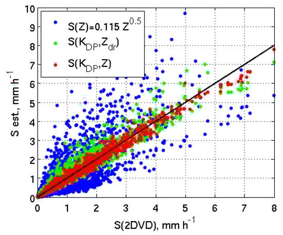
Figure 15.
Scatterplots of snow water equivalent rates measured by disdrometer during 16 Oklahoma snow events versus their estimates from the S(Z), S(KDP, Z), and S(KDP, Zdr) relations.
The biggest downside of the S(KDP, Z) snow estimator is its sensitivity to the shape and orientation factors Fs and Fo. This emphasizes the need for realistic assumptions about snow particles’ shapes and orientations either from in situ microphysical measurements or from polarimetric radar retrievals. A possible alternative solution is to find radar relations that are not sensitive to the variability of shapes and orientations. Such relations based on the joint use of KDP and ZDR were first suggested by Ryzhkov et al. [87,88]). It can be shown that the ratio KDP/(1 − Zdr−1) (where ) is practically immune to the changes in particle shapes and orientations. The Nguyen et al. [89] study confirms that the theoretical IWC(KDP, Zdr) relation from [87,88] is very close to their empirical relation derived from the side-looking airborne X-band radar measurements of KDP and ZDR and in situ observations onboard the Convair-580 aircraft during the High Altitude Ice Crystals—High Ice Water Content (HAIC—HIWC) campaign. This served as a motivation for derivation of S(KDP, Zdr) relation using the theoretical IWC(KDP, Zdr) relation as a starting point.
Because snow rate is proportional to the product of IWC and average terminal velocity vs. (or ) of snowflakes according to Equation (16):
where Dm is the mean volume diameter of snowflakes and IWC and Dm are determined using formulas [10]:
and:
A formula for practical utilization has a form [99]:
Although relation Equation (23) is immune to the variability of shapes and orientations, it is somewhat sensitive to the degree of riming quantified by the factor αs in Equation (15). It is also quite vulnerable to possible biases of the ZDR measurements, especially if ZDR is low. Hence, relation Equation (23) is not recommended to be used if ZDR < 0.2–0.3 dB.
Capozzi et al. [102] utilized an almost identical approach (using T-matrix scattering simulations instead of Rayleigh approximation) as Bukovčić et al. [101] to derive X-band polarimetric radar relations for snowfall rates using KDP or a combination of KDP and Z. They obtained comparable results to the wavelength-scaled S(KDP, Z) relation from [101] using X-band radar measurements in southern Italy, confirming that combining KDP with Z or ZDR improves the accuracy of snowfall rate estimates compared with the Z-based relations, as demonstrated in the subsequent study of Bukovčić et al. [99].
Because KDP in snow is usually quite low and noisy, especially at S band, its additional spatial averaging is required to obtain reliable and stable estimates of KDP and S. Such averaging is implemented as part of the Quasi-Vertical Profiles (QVPs) technique introduced by Ryzhkov et al. [103] which prescribes azimuthal averaging of polarimetric radar variables measured at higher antenna elevations. Similar techniques such as range-defined QVPs (RD-QVP; [104]), enhanced vertical profiles (EVP; [105]), and columnar vertical profiles (CVPs; [106]) became recently available to address the noisiness of KDP and ZDR in snow.
3.3. Results of Observations
The performance of polarimetric algorithms for snow estimation is illustrated for a heavy snowfall event. This storm was a classical nor’easter named Stella, which occurred on 14–15 March 2017. The storm produced heavy snow throughout the inner mid-Atlantic and northeast US, causing hurricane-like wind gusts along the New England coast. Several daily snowfall records were broken (e.g., Binghamton, NY; Burlington, VT; Scranton, PA), with the total maximum of 42 in (~1 m) in West Winfield (NY). The storm ranked twelfth on the Regional Snowfall Index (RSI; [107]) and twenty-third on the Northeast Snowfall Impact Scale (NESIS; [108]), disrupting the daily routine of more than 60 million people.
Figure 16 shows an example of composite PPI of Z, KDP, ZDR, and cross-correlation coefficient ρhv measured by the KBGM WSR-88D radar at El = 0.5° during the storm. Specific differential phase KDP exhibits inherent noisiness which, nevertheless, does not prevent to reveal a definite spatial structure with KDP enhancement in the area that does not coincide with the region of increased Z. Aggressive azimuthal averaging implemented in the RD-QVP methodology helps to significantly reduce the noisiness of KDP (see Figure 17).
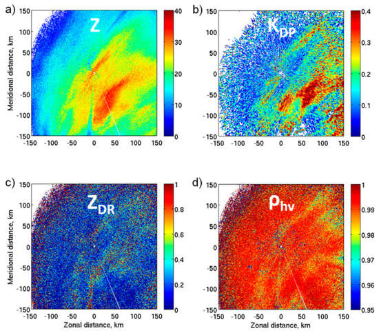
Figure 16.
Composite PPI of (a) Z, (b) KDP, (c) ZDR, and (d) ρhv at El = 0.5° measured by the KBGM WSR-88D radar in the Stella snowstorm on 14 March 2017 at 1256 UTC.
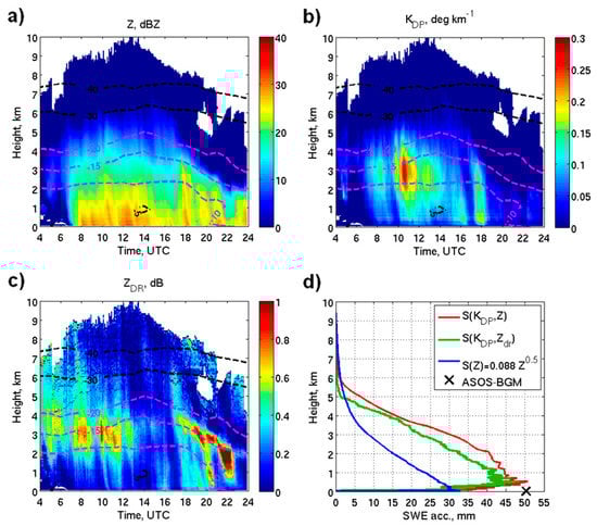
Figure 17.
KBGM radar RD-QVPs of (a) Z, (b) KDP, and (c) ZDR; the black dashed lines are isotherms, where the layer from −10 °C to −20 °C highlighted in magenta designates DGL; (d) profiles of SWE accumulations from the S(KDP, Z) (red line), S(KDP, Zdr) (green line), S(Z) (blue line), and KBGM ASOS accumulation estimate from the extinction coefficient measurements (black cross, co-located with radar); 14 March 2017.
The range-defined quasi-vertical profiles (RD-QVPs) of Z, KDP, and ZDR in a height-vs-time format obtained from the KBGM WSR-88D radar and vertical profiles of radar-retrieved snow water equivalent (SWE) accumulations are presented in Figure 17. The RD-QVP radar data were azimuthally averaged in a 15-km-radius circular area centered on the radar. Dashed lines indicate temperature isotherms obtained from the RAP model. Moderate to heavy snowfall rates persisted from 0700 to 1500 UTC, with a few intense snow bands later in the event. During these periods, the RD-QVP of Z exhibited elevated values greater than 30 dBZ (Figure 17a). Enhanced values of KDP and especially ZDR (Figure 17b,c) are noticeable in the dendritic growth layer (DGL) centered at about −15 °C. Such enhancements occasionally extended all the way to the ground (e.g., from 0700 to 1330 UTC). This marked a period of moderate concentration of smaller and denser dendrite-type crystals with a lower degree of aggregation at the surface. These can occasionally be mixed with the irregular-shape crystals, indicated by the enhanced values of KDP aloft (~1030 to 1130 UTC). This KDP increase, caused by high concentrations of irregular-shape crystals, comes as a precursor to the biggest low-level increase in Z, which shows a promising potential for snow nowcasting. In the later storm stages (1900 UTC onward) temperatures and cloud-top heights decrease, and the pristine dendrite-type crystals which do not aggregate, almost perfectly align with the −15 °C isotherm. These are also seen as ZDR streaks reaching the ground at 2010 and 2210 UTC. Previous observational studies [109,110] saw similar signatures in their data.
Three algorithms were used to estimate total SWE accumulation profiles from the RD-QVP data. These include the S(Z) = 0.088Z0.5 relation which is commonly used for the northeast US and polarimetric Relations (19) and (23) assuming that the particle aspect ratio is 0.6 and the canting angle spread σ is 20°. Actual SWE total accumulation at the surface of about 50 mm was measured by the Automatic Surface Observations Station (ASOS) in the close proximity to the KBGM radar. Both polarimetric estimates (red and green lines in Figure 17d) show more realistic representation of the vertical profile of accumulated SWE. The S(Z) relation produces apparent underestimation of snowfall (blue line in Figure 17d). Polarimetric relations are in accord with the notion that the bulk of precipitation (about 80 to 90%) is formed in the DGL ([111]). On the contrary, S(Z) produces about 40% of its total accumulation within the DGL (from ~2.0 to 4.5 km AGL) and moderately underestimates surface snow measurements (32 vs. 50 mm). Polarimetric relations at the lowest usable KDP height level (about 450 m AGL) yield results which are very close to the surface ASOS measurements.
Instantaneous snowfall rates and accumulations show more detailed pictures about the temporal evolution of these estimates (Figure 18). The standard S(Z) relation moderately underestimates snowfall rates throughout the event, with peaks not greater than 3 mm h−1 (gauge maximum is 5.5 mm/h). Polarimetric relations are in good agreement with the gauge, especially S(KDP, Z), which more accurately reproduce the peaks in rates. Strong winds (>7 m/s) were reported after 2000 UTC, where the minor degradation is seen in polarimetric relations estimations. In the strong wind situations, particles have more random motions and appear quasi-spherical, negatively impacting KDP (and ZDR). Polarimetric-based accumulations are in good agreement with the gauge estimate whereas the S(Z) relation underestimates the SWE amounts by about 40%. Additional examples of polarimetric measurements of snow can be found in [99].
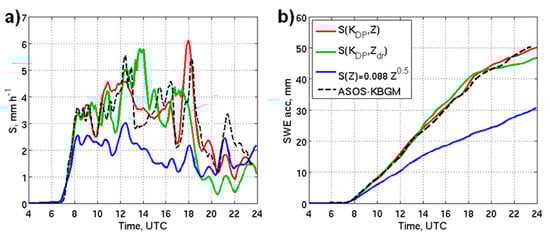
Figure 18.
Instantaneous snowfall rates (mm h−1) (a) from the KBGM ASOS extinction coefficient estimates (black dashed curve; ground), and radar RD-QVP estimates from S(KDP, Z) (red line; 0.5 km AGL), S(KDP, Zdr) (green line; 0.5 km AGL), S(Z) (blue line; 0.05 km AGL); respective SWE accumulations (mm) (b) from; 14 March 2017.
3.4. Discussion
Although the results of polarimetric estimation of snow in a limited number of cases are encouraging, they reveal obvious challenges as well. There is little doubt that the use of multiparameter polarimetric relations significantly reduces the impact of the PSD variability in snow. However, the S(KDP, Z) estimates are sensitive to the variability of particle shapes and orientations which are not known apriori. This variability does not affect the S(KDP, ZDR) estimates but these are much more affected by the uncertainty in snow density or degree of riming. A common problem for both polarimetric relations is that they cannot be directly applied for heavily aggregated dry snow where KDP and ZDR are vanishingly small and noisy. If KDP drops below 0.01–0.03 deg/km and ZDR are below 0.2–0.3 dB, the polarimetric estimates of snow become very unstable. This may limit the efficiency of polarimetric radar estimates in “warm” snow with temperatures just slightly below 0 °C. One possibility to address this issue is to resort to the polarimetric estimates of snow rate at higher altitudes and lower temperatures where KDP (or ZDR) are sufficiently high and project these estimates down to the surface assuming either conservation of the snow flux or predicting its downward evolution using simple cloud models as discussed in [112]. An alternative option is to switch to the S(Z) relation optimized for a certain snow type in areas of unreliable KDP and ZDR [83]. Note that the polarimetric snow relations are expected to perform better at shorter radar wavelengths (e.g., at C and X bands) for which KDP is higher and can be measured more reliably compared with S band.
Summarizing, we can conclude that, as opposed to the polarimetric methods for rainfall estimation which are quite mature and operationally usable, the algorithms for polarimetric snow measurements are still in their infancy and require substantial refinement and testing on a larger number of snow events.
4. Operational Implementation—MRMS QPE
Since the polarimetric upgrade of the US WSR-88D network, several QPE methodologies based on polarimetric radar variables have been developed for operations in the US National Weather Service (NWS). On the single radar applications, a hydrometeor classification algorithm (HCA, [113]) and an R(Z, ZDR), R(KDP) and R(Z) synthetic QPE [8] were developed and implemented in the operational WSR-88D Open Radar Product Generation (ORPG) system. The single radar synthetic QPE was later upgraded to an R(A) [42], R(Z, ZDR), R(KDP) and R(Z) synthetic QPE. On the multi-radar mosaic applications, a dual-pol (DP) radar quality control (dpQC) [114,115] to remove non-hydrometeor echoes and an R(A), R(KDP) and R(Z) synthetic QPE [26,46,47] were implemented in the Multi-Radar Multi-Sensor (MRMS, [9]) system. This section provides an overview of the DP radar synthetic QPE in the MRMS system.
Figure 19 shows an overview flowchart of the MRMS DP synthetic QPE process. The input data include DP radar moments and environmental data such as the 3D temperature field, freezing level height, and surface wet bulb temperature. The dpQC includes a simple correlation coefficient (ρhv) filter to separate hydrometeor (high ρhv) and non-hydrometeor (low ρhv) areas and a set of heuristic rules to handle exceptions to the simple ρhv filter. Such exceptions include areas of hail, non-uniform beam filling (NBF) and melting layer (ML) that have low ρhv values. Another exception is random clutter and biological pixels with high ρhv values. The dpQC uses 3D reflectivity structure and environmental data to protect hail, NBF, and ML areas from being removed by the simple ρhv filter, and it uses spatial filters and vertical and horizontal consistency checks to remove random non-precipitation pixels that exhibit high ρhv values. The dpQC removes more than 99% of non-hydrometeor echoes with very high computational efficiency [114].
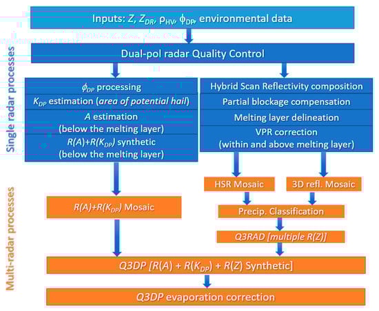
Figure 19.
An overview flowchart of the MRMS DP radar synthetic QPE.
After the dpQC, the differential phase ΦDP field is further processed for additional quality assurance. The ΦDP processing include four steps. The first step includes a speckle filter and a ρhv screening. The speckle filter checks for each ΦDP pixel and counts a number of non-missing ΦDP pixels in a 4.5 2.25 km box centered at the given pixel. If the number is less than 50% of the box total, then the given ΦDP pixel at the center is removed. A ρhv > 0.8 filter is applied to remove noisy and unreliable ΦDP data potentially associated with hail, severe NBF, or other residual contaminations after the dpQC. The second step unfolds ΦDP field based on the gate-to-gate ΦDP change and adjusts the unfolded ΦDP field to assure a monotonic increase trend with range. The third step applies a 6.25 km radial running mean through all non-missing ΦDP pixels to further reduce random errors and fluctuations. Finally, a linear interpolation along the radial is applied to fill in any gaps in the ΦDP field.
The specific differential phase KDP is calculated via a local linear fitting to ΦDP along the radial direction in areas where hail might be present. Specific attenuation A along the propagation path (r1, r2) in rain is calculated following Equations (2)–(6). The distance r1 corresponds to the nearest gate to the radar with precipitation and r2, to the last precipitation gate or the gate just below the bottom of the apparent melting layer (ML), whichever is closer to the radar. The ML is delineated using a scheme similar to [116] but its bottom and top were further expanded based on ρHV and Z to encompass all pixels potentially impacted by the ML. Pixels in [r1, r2] with potential hail contamination are excluded from the PIA calculation.
In the scheme currently implemented on the WSR-88D network, the factor α in Equation (6) is estimated from the 0.5 tilt data using the “ZDR-slope” K:
where K is a linear fit to the median ZDR values of each 2 dBZ reflectivity bin within the 20–50 dBZ range (Figure 20). Equation (24) was obtained from disdrometer data and supported by an analysis of ~10 events with a wide spread of moderate to heavy precipitation events from different geographical regimes. Figure 20 illustrates the process of α calculation. For the mesoscale convective system (MCS) near the KHTX WSR-88D radar (Figure 20a–c) on 11 December 2021, there was an apparent increase in ZDR with increasing Z, indicating the presence of large rain drops in the convective system. The ZDR-slope was relatively large (K = 0.048 dB/dBZ) and α was relatively low (0.0126 dB/deg) and close to those for convective rain [42,46,47]. For the Hurricane Ida case near the KMOB WSR-88D radar on 30 August 2021 (Figure 20d–f), the ZDR-slope was relatively flat (K = 0.017) and α (0.0361 dB/deg) was higher and closer to a tropical-type rain value.
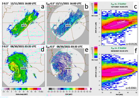
Figure 20.
Reflectivity Z (a,d), differential reflectivity ZDR (b,e) and Z–ZDR scatter plot (c,f) from KHTX (a–c) at 1600 UTC 11 Dec. 2021 and KMOB (d–f) at 0335 UTC 30 Aug. 2021. The black dots in (c,f) indicate median ZDR values, and the white dashed lines represent the linear fit to the median ZDR vs. Z.
Equation (24) is used to estimate α only if there are sufficient Z–ZDR data pairs in each 2-dBZ bin between 20 and 50 dBZ. If not enough Z–ZDR data pairs are found in the 20–50 dBZ interval, the number of Z–ZDR pairs in each 2-dBZ bin between 10 and 30 dBZ are checked. If significant data samples were found in the 10–30 dBZ interval, then the precipitation is considered pure stratiform and a default stratiform α (0.035 dB/deg) is applied. Otherwise, a new linear fit may be applied to the median ZDR values within the 10–40 dBZ range if sufficient Z–ZDR pairs were found in that range. If insufficient data pairs were found in the 10–40 dBZ reflectivity range, the precipitation is considered sporadic. A default convective (0.015 dB/deg) or stratiform (0.035 dB/deg) α is applied depending on the reflectivity intensities.
Once α is obtained and A calculated for each radar gate, precipitation rates are estimated from A on the 0.5° tilt in areas where reflectivity is below 45 dBZ (an adaptable parameter) using Equation (7). The 45 dBZ constraint is used to prevent R(A) from potential hail contamination. Above 50 dBZ (an adaptable parameter), two R(KDP) relationships are applied depending on the correlation coefficient, ρhv, field:
Equation (25) was derived using disdrometer measurements in the proximity of selected hailstorms in central Oklahoma, and Equation (26) provided optimal performance in heavy rain with large drops [6], also in central Oklahoma. Between 45 and 50 dBZ, a linear combination of R(A) and R(KDP) is applied to create a smooth transition between the two rates. The R(A) and R(KDP) are calculated from the 0.5° tilt currently with two additional constraints applied: (1) the beam blockage < 90% and (2) ΔΦDP 3°. If the blockage 90% or ΔΦDP < 3° at a given radial, the rate values for all the pixels in that radial are set to missing and R(Z), based rates are applied in the synthetic process at a later time (Figure 19).
Precipitation rate fields estimated via R(A) and R(KDP) from individual radars are mosaicked through a physically based scheme shown in [117]. Since R(A) is only valid below the melting layer, the mosaic may have gaps in areas far away from the radars. Figure 21a shows such a gap between KHTX and KMRX radars. To fill in these gaps, a multiple R(Z), based QPE (“Q3RAD”, Figure 21b) described in [9] was applied. A flowchart of the Q3RAD QPE is shown in the right half of Figure 19. After the QC, a 2D hybrid scan reflectivity (HSR) field is derived from the lowest radar bins with less than 50% blockages, and the reflectivity bins with blockages greater than 10% are adjusted to compensate for the power loss. The apparent melting layer is delineated for all the tilts based on a scheme similar to [118] and a vertical profile of reflectivity (VPR) correction was applied to the HSR field within and above the melting layer [61]. The HSR fields from individual radars are then mosaicked based on the methodology developed in [117]. A precipitation type field of seven categories (warm stratiform rain, cool stratiform rain, convective rain, tropical-stratiform rain mix, tropical-convective rain mix, hail, and snow) is generated using an automated precipitation classification described in [9]. Finally, multiple R(Z) relationships are applied to the HSR field according to the precipitation types to obtain the Q3RAD rate. The main Q3RAD R(Z) relationships applied in the warm season are as follows:
where β is a rate multiplier ranging from 1.0 to 1.5 depending on the month of the year and the proximity to frequent hurricane zones [9,118]. For the coastal areas of the Gulf of Mexico and Atlantics and southeastern US, β can be as high as 1.45 for September and 1.5 for October. The convective R(Z) was capped at a value that ranges from 53.8 mm/h to 150 mm/h depending on the climatological region and real-time hail size estimation. The cap is lower in areas of continental rain regime with severe hail and higher in areas of maritime warm rain and hurricanes.
Stratiform rain: Rstra = max (0.0365 Z0.625, 0.1155 Z0.5);
Convective rain: Rconv = 0.017 Z0.714;
Tropical rain: Rtrop = 0.010 β Z0.833
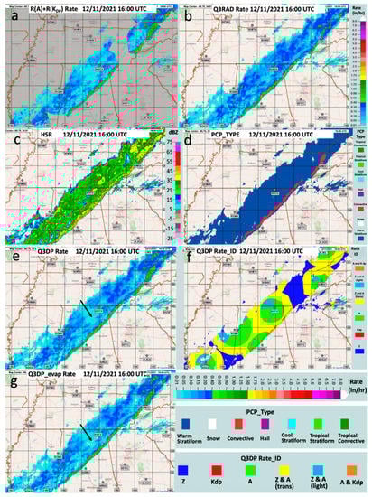
Figure 21.
(a) R(A) + R(KDP) rate mosaic, (b) multiple R(Z) rate, (c) hybrid scan reflectivity mosaic, (d) precipitation type, (e) the R(A) + R(KDP) + R(Z) DP synthetic QPE, (f) the DP synthetic QPE categories, and (g) the DP synthetic QPE with evaporation correction, all valid at 1600 UTC 11 December 2021.
Figure 21c,d show the example of the HSR mosaic and precipitation type fields corresponding to the Q3RAD rate in Figure 21b. The final dual-pol radar synthetic QPE (“Q3DP”) is shown in Figure 21e,f which shows the contributing sources of the rates to the Q3DP from different relationships. The dark blue areas in Figure 21f indicate where Q3RAD fills in when the radar beam intersects or overshoots the melting layer and light blue when ΔΦDP < 3°. The yellow areas indicate a transition zone (default width: 50 km) near the outer boundary of R(A) where a weighted mean of the R(A) and R(Z) rates is applied to prevent discontinuities between the two. The red areas indicate where R(KDP) is applied and orange the linear transition between R(A) and R(KDP). Finally, an evaporation correction is applied to the mosaicked precipitation rate field based on the methodology provided by Martinaitis et al. [119]. The correction factor is a function of the rate, the height of the radar estimate, and atmospheric properties between the radar data height and the ground. The correction helps reducing false light precipitation in the radar QPE due to virga. Figure 21g shows the same Q3DP rate field as in Figure 21e but with the evaporation correction.
Q3DP was evaluated across CONUS during the period of 15 September–31 October 2018. The Community Collaborative Rain, Hail and Snow Network, www.cocorahs.org/, (accessed on 1 February 2022) (CoCoRaHS) rain gauges were used to compare the performances of the Q3DP and Q3RAD 24-h QPEs. The statistic scores for both QPE techniques for different rainfall categories are summarized in Table 2. The categories are subjectively defined as very light (VL: G < 0.5 in.), light (L: 0.5 G 1 in.), moderate (M: 1 G < 2 in.), heavy (H: 2 G < 4 in.), and very heavy (VH: G 4 in.).
Table 2.
Mean bias ratio (MBR), correlation coefficient (CC), mean absolute error (MAE) and fractional MAE of the Q3RAD and Q3DP 24 h QPEs for predefined 24 h rainfall categories. The bold numbers indicate the better scores among the two products.
Q3DP showed a reduction in systematic bias and random errors over Q3RAD, especially for the heavy amounts higher than 2 in., Q3RAD had a 19% overestimation bias in the VL rain and 18%, 20%, and 19% underestimation biases in the M, H, and VH rain, respectively. Q3DP reduced the biases by 15%, 6%, 12%, and 16% for VL, M, H, and VH categories, respectively, and remained the same for the L category. A similar trend was found in the MAE score, where Q3DP reduced the errors for VL, M, H, and VH categories but slightly increased the error in the L category. For the correlation coefficient, Q3DP was about the same as Q3RAD in the VL and L and was higher in the M–VH categories. Q3DP showed a significantly reduced uncertainty with respect to Q3RAD for rainfall amounts. The reduced uncertainty in Q3DP was also reflected in its lower MAEs/fMAEs for the H and VH categories. Q3DP reduced the fMAE by 6%, 7%, and 11% for the VL, H, and VH categories, respectively, while the fMAEs of Q3DP and Q3RAD for the L and M categories remained similar.
5. Conclusions
A primary outcome of the radar rainfall estimation research during last two decades is the realization that the polarimetric methodologies based on the use of specific attenuation A and specific differential phase KDP have undeniable benefits compared with the techniques that utilize either a single radar reflectivity factor Z or a combination of Z with differential reflectivity ZDR. This is attributed to lower sensitivity of the R(A) and R(KDP) relations to the DSD variability and immunity of the estimates of A and KDP to the radar calibration errors, attenuation in rain, partial beam blockage, and impact of wet radome. These benefits are well-proven for all three S-, C-, and X-microwave frequency bands at which polarimetric weather surveillance radars operate. It is demonstrated that the composite rainfall algorithms utilizing R(A) relations for lower rain rates and R(KDP) relations for heavier rain show the best performance. The A-based methods are particularly advantageous at S band because the S-band R(A) relation is almost linear and can be utilized in a wider range of rain intensities compared with C and X bands.
There is still room for additional optimization of the R(A) and R(KDP) algorithms to further mitigate their residual sensitivity to the DSD variability. At S band, this must be performed by optimizing the parameter α = A/KDP in the estimation of A and the multiplier in the power-law R(KDP) relation.
Notable progress was achieved in mitigation of the impact of the “bright band” contamination on the surface rainfall estimates at longer distances from the radar using polarimetric VPR correction (PVPR) although these techniques require more testing and refinement. Taking into the account the vertical profiles of reflectivity below the melting layer and above, is a subject of ongoing research.
The algorithms for polarimetric measurements of snow were recently introduced and show good promise as was demonstrated at S band. They utilize combinations of Z and KDP or KDP and ZDR and may produce even better results at C and X bands due to higher value of KDP at shorter radar wavelengths. A common problem for this methodology is a reduced value of KDP in dry aggregated snow near the surface and the inherent uncertainty related to the KDP dependency on the shapes and orientations of snowflakes.
The advanced polarimetric radar QPE methods utilizing the R(A), R(KDP), and R(Z) relations were implemented on the operational network of the WSR-88D radars in the US using the Multi-Radar Multi-Sensor (MRMS) platform that integrates rainfall estimates from all operational radars and provides comparison of radar rainfall products with dense networks of rain gauges.
With all the progress achieved during last two decades, a number of challenges and opportunities remains. These include the need to improve the rainfall estimation performance at longer distances from the radar, further development of the algorithms for polarimetric quantification of snow, and more aggressive utilization of the methodologies involving artificial intelligence/machine learning.
Author Contributions
A.R. wrote Section 1, Section 2, and Section 5 and performed an overall editing of the manuscript; P.Z. provided most of the radar data and plots for Section 2; P.B. wrote Section 3, and J.Z. and S.C. wrote Section 4 of the manuscript. All authors have read and agreed to the published version of the manuscript.
Funding
This work was largely supported by the National Weather Service Radar Operations Center’s NEXRAD Product Improvement and Technical Transfer programs and the funding was provided through the NOAA/Office of Oceanic and Atmospheric Research under the NOAA—University of Oklahoma Cooperative Agreements NA16OAR4320115 and NA21OAR4320204, U.S. Department of Commerce.
Institutional Review Board Statement
Not applicable.
Informed Consent Statement
Not applicable.
Data Availability Statement
All data are available upon request.
Conflicts of Interest
The authors declare no conflict of interest.
References
- Ryzhkov, A.; Zrnic, D. Comparison of dual-polarization radar estimators of rain. J. Atmos. Ocean. Technol. 1995, 12, 249–256. [Google Scholar] [CrossRef]
- Ryzhkov, A.; Zrnic, D. Assessment of rainfall measurement that uses specific differential phase. J. Appl. Meteorol. 1996, 35, 2080–2090. [Google Scholar] [CrossRef]
- May, P.; Keenan, T.; Zrnic, D.; Carey, L.; Rutledge, S. Polarimetric radar measurements of tropical rain at 5-cm wavelength. J. Appl. Meteorol. 1999, 38, 750–765. [Google Scholar] [CrossRef]
- Testud, J.; Le Bouar, E.; Obligis, E.; Ali-Mehenni, M. The rain profiling algorithm applied to polarimetric weather radar. J. Atmos. Ocean. Technol. 2000, 17, 332–356. [Google Scholar] [CrossRef]
- Brandes, E.; Zhang, G.; Vivekanandan, J. Experiments in rainfall estimation with a polarimetric radar in a subtropical environment. J. Appl. Meteorol. 2002, 41, 674–685. [Google Scholar] [CrossRef]
- Ryzhkov, A.; Giangrande, S.; Schuur, T. Rainfall estimation with a polarimetric prototype of the WSR-88D radar. J. Appl. Meteorol. 2005, 44, 502–515. [Google Scholar] [CrossRef]
- Matrosov, S.; Kingsmill, D.; Ralph, F. The utility of X-band polarimetric radar for quantitative estimates of rainfall parameters. J. Hydrometeorol. 2005, 6, 248–262. [Google Scholar] [CrossRef]
- Ryzhkov, A.; Schuur, T.; Burgess, D.; Giangrande, S.; Zrnic, D. The Joint Polarization Experiment: Polarimetric rainfall measurements and hydrometeor classification. Bull. Am. Meteorol. Soc. 2005, 86, 809–824. [Google Scholar] [CrossRef]
- Zhang, J. and Coauthors. Multi-Radar Multi-Sensor (MRMS) quantitative precipitation estimation: Initial operating capabilities. Bull. Am. Meteorol. Soc. 2016, 97, 621–638. [Google Scholar] [CrossRef]
- Ryzhkov, A.; Zrnic, D. Radar Polarimetry for Weather Observations; Springer Atmospheric Sciences: Cham, Switzerland, 2019; p. 486. [Google Scholar]
- Seliga, T.; Bringi, V.; Al-Khatib, H. A preliminary study of comparative measurement of rainfall rate using the differential reflectivity radar technique and a raingauge network. J. Appl. Meteorol. 1981, 20, 1362–1368. [Google Scholar] [CrossRef]
- Schuur, T.; Ryzhkov, A.; Clabo, D. Climatological analysis of DSDs in Oklahoma as revealed by 2D-video disdrometer and polarimetric WSR-88D. In Proceedings of the 32nd Conference Radar Meteorology, Albuquerque, NM, USA, 24–29 October 2005; American Meteorology Society: Boston, MA, USA, 2005; Volume 15. [Google Scholar]
- Giangrande, S.; Ryzhkov, A. Estimation of rainfall based on the results of polarimetric echo classification. J. Appl. Meteorol. 2008, 47, 2445–2462. [Google Scholar] [CrossRef]
- Cifelli, R.; Chandrasekar, V.; Lim, S.; Kennedy, P.; Wang, Y.; Rutledge, S. A new dual-polarization radar rainfall algorithm: Application in Colorado precipitation events. J. Atmos. Ocean. Technol. 2011, 28, 352–364. [Google Scholar] [CrossRef]
- Pepler, A.; May, P.; Thurai, M. A robust error-based rain estimation method for polarimetric radar. Part I: Development of a method. J. Appl. Meteorol. Clim. 2011, 50, 2092–2103. [Google Scholar] [CrossRef]
- Bringi, V.; Rico-Ramirez, M.; Thurai, M. Rainfall estimation with an operational polarimetric C-band radar in the United Kingdom: Comparison with a gage network and error analysis. J. Hydrometeorol. 2011, 12, 935–954. [Google Scholar] [CrossRef]
- Chen, H.; Chandrasekar, V.; Bechini, R. An improved dual-polarization radar rainfall algorithm (DROPS2.0): Application in NASA IFloodS field campaign. J. Hydrometeorol. 2017, 18, 917–937. [Google Scholar] [CrossRef]
- Chen, G.; Kun, Z.; Zhang, G.; Hao, H.; Liu, S.; Wen, L.; Yang, Z.; Yang, Z.; Xu, L.; Zhu, W. Improving Polarimetric C-Band Radar Rainfall Estimation with Two-Dimensional Video Disdrometer Observations in Eastern China. J. Hydrometeorol. 2017, 18, 1375–1391. [Google Scholar] [CrossRef]
- Thompson, E.; Rutledge, S.; Dolan, B.; Thurai, M.; Chandrasekar, V. Dual-polarization radar rainfall estimation over tropical oceans. J. Appl. Meteorol. Climatol. 2018, 57, 755–775. [Google Scholar] [CrossRef]
- Chen, J.-Y.; Troemel, S.; Ryzhkov, A.; Simmer, C. Assessing the benefits of specific attenuation for quantitative precipitation estimation with a C-band radar network. J. Hydrometeorol. 2021, 22, 2617–2631. [Google Scholar] [CrossRef]
- Matrosov, S.; Cifelli, R.; Kennedy, P.; Nesbitt, S.; Rutledge, S.; Bringi, V.; Martner, B. A comparative study of rainfall retrievals based on specific differential phase shifts at X- and S-band frequencies. J. Atmos. Ocean. Technol. 2006, 23, 952–963. [Google Scholar] [CrossRef]
- Ryzhkov, A.; Zrnic, D.; Fulton, R. Areal Rainfall Estimates Using Differential Phase. J. Appl. Meteorol. 2000, 39, 263–268. [Google Scholar] [CrossRef]
- Borowska, L.; Zrnic, D.; Ryzhkov, A.; Zhang, P.; Simmer, C. Polarimetric estimates of a 1-month accumulation of light rain with a 3-cm wavelength radar. J. Hydrometeorol. 2011, 12, 1024–1039. [Google Scholar] [CrossRef]
- Balakrishnan, N.; Zrnic, D. Estimation of rain and hail rates in mixed-phase precipitation. J. Atmos. Sci. 1990, 47, 565–583. [Google Scholar] [CrossRef]
- Kumjian, M.; Lebo, Z.; Ward, A. Storms producing large accumulations of small hail. J. Appl. Meteorol. Climatol. 2019, 58, 341–364. [Google Scholar] [CrossRef]
- Zhang, J.; Tang, L.; Cocks, S.; Zhang, P.; Ryzhkov, A.; Howard, K.; Langston, C.; Kaney, B. A dual-polarization radar synthetic QPE for operations. J. Hydrometeorol. 2020, 21, 2507–2521. [Google Scholar] [CrossRef]
- Sachidananda, M.; Zrnic, D. Rain rate estimates from differential polarization measurements. J. Atmos. Ocean. Technol. 1987, 4, 588–598. [Google Scholar] [CrossRef]
- Park, S.-G.; Maki, M.; Iwanami, K.; Bringi, V.; Chandrasekar, V. Correction of radar reflectivity and differential reflectivity for rain attenuation at X band. Part II: Evaluation and application. J. Atmos. Ocean. Technol. 2005, 22, 1633–1655. [Google Scholar]
- Bringi, V.; Thurai, M.; Nakagawa, K.; Huang, G.; Kobayashi, T.; Adachi, A.; Hanado, H.; Sekizawa, S. Rainfall estimation from C-band polarimetric radar in Okinawa, Japan: Comparisons with 2D-video disdrometer and 400 MHz wind profiler. J. Meteorol. Soc. Jpn. 2006, 84, 705–724. [Google Scholar] [CrossRef]
- Matrosov, S. Evaluating polarimetric X-band radar rainfall estimators during HMT. J. Atmos. Ocean. Technol. 2010, 27, 122–134. [Google Scholar] [CrossRef]
- Wang, Y.; Chandrasekar, V. Quantitative precipitation estimation in the CASA X-band dual-polarization radar network. J. Atmos. Ocean. Technol. 2010, 27, 1665–1676. [Google Scholar] [CrossRef]
- Anagnostou, M.; Kalogiros, J.; Anagnostou, E.; Tarolli, M.; Papadopoulos, A.; Borga, M. Performance evaluation of high-resolution estimation from X-band dual-polarization radar for flash flood applications in mountainous basins. J. Hydrol. 2010, 394, 4–16. [Google Scholar] [CrossRef]
- Tabary, P.; Boumahmoud, A.; Andrieu, H.; Thompson, R.; Illingworth, A.; LeBouar, E.; Testud, J. Evaluation of two “integrated” polarimetric quantitative precipitation estimation (QPE) algorithms at C band. J. Hydrol. 2011, 405, 248–260. [Google Scholar] [CrossRef]
- Vulpiani, G.; Montopoli, M.; Passeri, L.; Giola, A.; Giordano, P.; Marzano, F. On the use of dual-polarized C-band radar for operational rainfall retrieval in mountaneous areas. J. Appl. Meteorol. Clim. 2012, 51, 405–425. [Google Scholar] [CrossRef]
- Matrosov, S.; Cifelli, R.; Gochis, D. Measurements of heavy convective rainfall in presence of hail in flood-prone areas using an X-band polarimetric radar. J. Appl. Meteorol. Clim. 2013, 52, 395–407. [Google Scholar] [CrossRef]
- Figueras, I.; Ventura, J.; Tabary, P. The new French operational polarimetric radar rainfall rate product. J. Appl. Meteorol. Clim. 2013, 52, 1817–1835. [Google Scholar] [CrossRef]
- Wang, Y.; Zhang, J.; Ryzhkov, A.; Tang, L. C-band polarimetric radar QPE based on specific differential propagation phase for extreme typhoon rainfall. J. Atmos. Ocean. Technol. 2013, 30, 1354–1370. [Google Scholar] [CrossRef]
- Chen, H.; Chandrasekar, V. The quantitative precipitation estimation system for Dallas—Fort Worth (DFW) urban remote sensing network. J. Hydrol. 2015, 531, 259–271. [Google Scholar] [CrossRef]
- Diederich, M.; Troemel, S.; Ryzhkov, A.; Zhang, P.; Simmer, C. Use of specific attenuation for rainfall measurements at X-band radar wavelengths. Part II: Rainfall estimates and comparison with rain gauges. J. Hydrometeorol. 2015, 16, 503–516. [Google Scholar] [CrossRef]
- Huang, H.; Zhao, K.; Zhang, G.; Lin, Q.; Wen, L.; Chen, G.; Yang, Z.; Wang, M.; Hu, D. Quantitative precipitation estimation with operational polarimetric radar measurements in southern China: A differential phase–based variational approach. J. Atmos. Ocean. Technol. 2018, 35, 1253–1271. [Google Scholar] [CrossRef]
- Chen, J.; Chang, W.-Y.; Chang, P.-L. A synthetic quantitative precipitation estimation by integrating S- and C-band dual-polarization radars over Northern Taiwan. Remote Sens. 2021, 13, 154. [Google Scholar] [CrossRef]
- Ryzhkov, A.; Diederich, M.; Zhang, P.; Simmer, C. Utilization of specific attenuation for rainfall estimation, mitigation of partial beam blockage, and radar networking. J. Atmos. Ocean. Technol. 2014, 31, 599–619. [Google Scholar] [CrossRef]
- Giangrande, S.; Collis, S.; Theisen, A.; Tokay, A. Precipitation estimation from the ARM distributed radar network during the MC3E campaign. J. Appl. Meteorol. Climatol. 2014, 53, 2130–2147. [Google Scholar] [CrossRef][Green Version]
- Wang, Y.; Zhang, P.; Ryzhkov, A.; Zhang, J.; Chang, P.-L. Utilization of specific attenuation for tropical rainfall estimation in complex terrain. J. Hydrometeorol. 2014, 15, 2250–2266. [Google Scholar] [CrossRef]
- Boodoo, S.; Hudak, D.; Ryzhkov, A.; Zhang, P.; Donaldson, N.; Sills, D.; Reid, J. Quantitative precipitation estimation from a C-Band Dual-polarized radar for the 8 July 2013 flood in Toronto, Canada. J. Hydrometeorol. 2015, 16, 2027–2044. [Google Scholar] [CrossRef]
- Wang, Y.; Cocks, S.; Tang, L.; Ryzhkov, A.; Zhang, P.; Zhang, J.; Howard, K. A prototype quantitative precipitation estimation algorithm for operational S-band polarimetric radar utilizing specific attenuation and specific differential phase: Part I–Algorithm description and initial results. J. Hydrometeorol. 2019, 20, 985–997. [Google Scholar] [CrossRef]
- Cocks, S.; Wang, Y.; Tang, L.; Ryzhkov, A.; Zhang, P.; Zhang, J.; Howard, K. A prototype quantitative precipitation estimation algorithm for operational S-band polarimetric radar utilizing specific attenuation and specific differential phase: Part II–Case study analysis and performance verification. J. Hydrometeorol. 2019, 20, 999–1014. [Google Scholar] [CrossRef]
- Seo, B.; Ryzhkov, A.; Krajewski, W. Evaluation of the specific attenuation method for radar-based quantitative precipitation estimation: Improvements and practical challenges. J. Hydrometeorol. 2020, 21, 1333–1347. [Google Scholar] [CrossRef]
- Huang, H.; Zhao, K.; Chen, H.; Hu, D.; Fu, P.; Lin, Q.; Yang, Z. Improved attenuation-based radar precipitation estimation considering the azimuthal variabilities of microphysical properties. J. Hydrometeorol. 2020, 21, 1605–1620. [Google Scholar] [CrossRef]
- Zhang, P.; Zrnic, D.; Ryzhkov, A. Partial beam blockage correction using polarimetric radar measurements. J. Atmos. Ocean. Technol. 2013, 30, 861–872. [Google Scholar] [CrossRef]
- Kitchen, M.; Brown, R.; Davies, A. Real-time correction of weather radar data for the effects of bright band, range and orographic growth in widespread precipitation. Q. J. R. Meteorol. Soc. 1994, 120, 1231–1254. [Google Scholar] [CrossRef]
- Seo, D.-J.; Breidenbach, J.; Fulton, R.; Miller, D.; O’Bannon, T. Real-time adjustment of range-dependent biases in WSR-88D rainfall estimates due to nonuniform vertical profile of reflectivity. J. Hydrometeorol. 2000, 1, 222–240. [Google Scholar] [CrossRef]
- Germann, U.; Joss, J. Mesobeta profiles to extrapolate radar precipitation measurements above the Alps to the ground level. J. Appl. Meteorol. 2002, 41, 542–557. [Google Scholar] [CrossRef]
- Matrosov, S.; Clark, K.; Kingsmill, D. A polarimetric radar approach to identify rain, melting-layer, and snow regions for applying corrections to vertical profiles of reflectivity. J. Appl. Meteorol. Climatol. 2007, 46, 154–166. [Google Scholar] [CrossRef]
- Koistinen, J. Operational correction of radar rainfall errors due to vertical reflectivity profile. In Proceedings of the 25th International Conference on Radar Meteorology, Paris, France, 24–28 June 1991; American Meteorology Society: Boston, MA, USA, 1991; Volume 91, p. 94. [Google Scholar]
- Andrieu, H.; Creutin, J. Identification of vertical profiles of radar reflectivity for hydrological applications using an inverse method. Part I: Formulation. J. Appl. Meteorol. Climatol. 1995, 34, 225–239. [Google Scholar] [CrossRef]
- Andrieu, H.; Delrieu, G.; Creutin, J. Identification of vertical profiles of radar reflectivity for hydrological applications using an inverse method. Part II: Sensitivity analysis and case study. J. Appl. Meteor. 1995, 34, 240–259. [Google Scholar] [CrossRef]
- Vignal, B.; Andrieu, H.; Creutin, J. Identification of vertical profiles of reflectivity from volume-scan radar data. J. Appl. Meteor. 1999, 38, 1214–1228. [Google Scholar] [CrossRef]
- Vignal, B.; Galli, G.; Joss, J.; Germann, U. Three methods to determine profiles of reflectivity from volumetric radar data to correct precipitation estimates. J. Appl. Meteor. 2000, 39, 1715–1726. [Google Scholar] [CrossRef]
- Vignal, B.; Krajewski, W. Large-sample evaluation of two methods to correct range-dependent error for WSR-88D rainfall estimates. J. Hydrometeorol. 2001, 2, 490–504. [Google Scholar] [CrossRef]
- Zhang, J.; Qi, Y. A Real-Time Algorithm for the Correction of Brightband Effects in Radar-Derived QPE. J. Hydrometeorol. 2010, 11, 1157–1171. [Google Scholar] [CrossRef]
- Qi, Y.; Zhang, J.; Zhang, P.; Cao, Q. VPR correction of bright band effects in radar QPEs using polarimetric radar observations. J. Geophys. Res. Atmos. 2013, 118, 3627–3633. [Google Scholar] [CrossRef]
- Hanft, W.; Zhang, J. Dual-pol VPR corrections for improved operational radar QPE in MRMS. J. Hydrometeorol. 2022, Submitted. [Google Scholar]
- Ryzhkov, A.; Krause, J. New polarimetric radar algorithm for melting layer detection and determination of its height. J. Atmos. Ocean. Technol. 2022, in press. [Google Scholar]
- Zhang, Y.; Bi, S.; Liu, L.; Chen, H.; Zhang, Y.; Shen, P.; Yang, F.; Wang, Y.; Zhang, Y.; Yao, S. Deep learning for polarimetric radar quantitative precipitation estimation during landfalling typhoons in South China. Remote Sens. 2021, 13, 3157. [Google Scholar] [CrossRef]
- Shin, K.; Song, J.; Bang, W.; Lee, G. Quantitative Precipitation Estimates using machine learning approaches with operational dual-polarization radar data. Remote Sens. 2021, 13, 694. [Google Scholar] [CrossRef]
- Wolfensberger, D.; Gabella, M.; Boscacci, M.; Germann, U.; Berne, A. RainForest: A random forest algorithm for quantitative precipitation estimation over Switzerland. Atmos. Meas. Tech. 2021, 14, 3169–3293. [Google Scholar] [CrossRef]
- Gunn, K.; Marshall, J. The distribution with size of aggregate snowflakes. J. Meteorol. 1958, 15, 452–461. [Google Scholar] [CrossRef]
- Sekhon, R.; Srivastava, R. Snow size spectra and radar reflectivity. J. Atmos. Sci. 1970, 27, 299–307. [Google Scholar] [CrossRef]
- Fujiyoshi, Y.; Endoh, T.; Yamada, T.; Tsuboki, K.; Tachibana, Y.; Wakahama, G. Determination of a Z–R relationship for snowfall using a radar and sensitive snow gauges. J. Appl. Meteorol. Climatol. 1990, 29, 147–152. [Google Scholar] [CrossRef]
- Matrosov, S. Modeling backscatter properties of snowfall at millimeter wavelengths. J. Atmos. Sci. 2007, 64, 1727–1736. [Google Scholar] [CrossRef]
- Matrosov, S.; Campbell, C.; Kingsmill, D.; Sukovich, E. Assessing snowfall rates from X-band radar reflectivity measurements. J. Atmos. Ocean. Technol. 2009, 26, 2324–2339. [Google Scholar] [CrossRef]
- Szyrmer, W.; Zawadzki, I. Snow studies. Part II: Average relationship between mass of snowflakes and their terminal fall velocity. J. Atmos. Sci. 2010, 67, 3319–3335. [Google Scholar] [CrossRef]
- Zhang, G.; Luchs, S.; Ryzhkov, A.; Xue, M.; Ryzhkova, L.; Cao, Q. Winter precipitation microphysics characterized by polarimetric radar and video disdrometer observations in central Oklahoma. J. Appl. Meteorol. Climatol. 2011, 50, 1558–1570. [Google Scholar] [CrossRef]
- Heymsfield, A.; Matrosov, S.; Wood, N. Toward improving ice water content and snow-rate retrievals from radars. Part I: X and W bands, emphasizing CloudSat. J. Appl. Meteorol. Climatol. 2016, 55, 2063–2090. [Google Scholar] [CrossRef]
- Huang, G.-J.; Bringi, V.; Cifelli, R.; Hudak, D.; Petersen, W. A methodology to derive radar reflectivity-liquid equivalent snow rate relations using C-band radar and a 2D video disdrometer. J. Atmos. Ocean. Technol. 2010, 27, 637–651. [Google Scholar] [CrossRef]
- Saltikoff, E.; Huuskonen, A.; Hohti, H.; Koistinen, J.; Jarvinen, H. Quality assurance in the FMI Doppler weather radar network. Boreal Environ. Res. 2010, 15, 579–594. [Google Scholar]
- Wolfe, J.; Snider, J. A relationship between reflectivity and snow rate for a high-altitude S-band radar. J. Appl. Meteorol. Climatol. 2012, 51, 1111–1128. [Google Scholar] [CrossRef]
- Huang, G.-J.; Bringi, V.; Moisseev, D.; Petersen, W.; Bliven, L.; Hudak, D. Use of 2D-video disdrometer to derive mean density-size and Ze–SR relations: Four snow cases from the light precipitation validation environment. Atmos. Res. 2015, 153, 34–48. [Google Scholar] [CrossRef]
- Von Lerber, A.; Moisseev, D.; Bliven, L.; Petersen, W.; Harri, A.; Chandrasekar, V. Microphysical properties of snow and their link to Ze–S relations during BAECC 2014. J. Appl. Meteorol. Clim. 2017, 56, 1561–1582. [Google Scholar] [CrossRef]
- Skofronick-Jackson, G.; Hudak, D.; Petersen, W.; Nesbitt, S.W.; Chandrasekar, V.; Durden, S.; Gleicher, K.J.; Huang, G.-J.; Joe, P.; Kollias, P.; et al. Global Precipitation Measurement Cold Season Precipitation Experiment (GCPEX). Bull. Am. Meteorol. Soc. 2015, 96, 1719–1741. [Google Scholar] [CrossRef]
- Huang, G.-J.; Bringi, V.; Newman, A.; Lee, G.; Moisseev, D.; Notaroš, B. Dual-wavelength radar technique development for snow rate estimation: A case study from GCPEx. Atmos. Meas. Tech. 2019, 12, 1409–1427. [Google Scholar] [CrossRef]
- Tiira, J.; Moisseev, D. Unsupervised classification of vertical profiles of dual polarization radar variables. Atmos. Meas. Tech. 2020, 13, 1227–1241. [Google Scholar] [CrossRef]
- Vivekanandan, J.; Bringi, V.; Hagen, M.; Meischner, P. Polarimetric radar studies of atmospheric ice particles. IEEE Trans. Geosci. Remote Sens. 1994, 32, 1–10. [Google Scholar] [CrossRef]
- Lu, Y.; Aydin, K.; Cothiaux, E.; Verlinde, J. Retrieving cloud ice water content using millimeter- and centimeter wavelength radar polarimetric observables. J. Appl. Meteorol. Climatol. 2015, 54, 596–604. [Google Scholar] [CrossRef]
- Aydin, K.; Tang, C. Estimation of ice water content with 94-GHz millimeter wave radar observables. In Proceedings of the 1995 27th Conference on Radar Meteorology, Vail, CO, USA, 9–13 October 1995; American Meteorological Soc.: Boston, MA, USA, 1995; pp. 550–552. [Google Scholar]
- Ryzhkov, A.; Zrnic, D.; Gordon, B. Polarimetric method for ice water content determination. J. Appl. Meteorol. 1998, 37, 125–134. [Google Scholar] [CrossRef]
- Ryzhkov, A.; Bukovcic, P.; Murphy, A.; Zhang, P.; McFarquhar, G. Ice microphysical retrievals using polarimetric radar data. In Proceedings of the 10th European Conference on Radar in Meteorology and Hydrology, Wageningen, The Netherlands, 1–6 July 2018. [Google Scholar]
- Nguyen, C.; Wolde, M.; Korolev, A. Determination of ice water content (IWC) in tropical convective clouds from X-band dual-polarization airborne radar. Atmos. Meas. Tech. 2019, 12, 5897–5911. [Google Scholar] [CrossRef]
- Bukovčić, P.; Ryzhkov, A.; Carlin, J. Polarimetric Radar Relations for Estimation of Visibility in Aggregated Snow. J. Atmos. Ocean. Technol. 2021, 38, 805–822. [Google Scholar] [CrossRef]
- Poljakova, E.; Tretjakov, V. Visibility in falling snow. Trudy Gl. Geofiz. Obs. 1960, 100, 53–57. [Google Scholar]
- Warner, C.; Gunn, K. Measurement of snowfall by optical attenuation. J. Appl. Meteorol. Climatol. 1969, 8, 110–121. [Google Scholar] [CrossRef][Green Version]
- Muench, H.; Brown, H. Measurements of Visibility and Radar Reflectivity during Snowstorms in the AFGL Mesonet; NASA STI/Recon Tech. Rep.; NASA: Washington, DC, USA, 1977; Volume 78, 34p. [Google Scholar]
- Fujiyoshi, Y.; Wakahamam, G.; Endoh, T.; Irikawa, S.; Konishi, H.; Takeuchi, M. Simultaneous observation of snowfall intensity and visibility in winter at Sapporo. Low Temp. Sci. 1983, 42A, 147–156. [Google Scholar]
- Rasmussen, R.; Vivekanandan, J.; Cole, J.; Myers, B.; Masters, C. The estimation of snowfall rate using visibility. J. Appl. Meteor. 1999, 38, 1542–1563. [Google Scholar] [CrossRef]
- Boudala, F.; Isaac, G. Parameterization of visibility in snow: Application in numerical weather prediction models. J. Geophys. Res. 2009, 114, D19202. [Google Scholar] [CrossRef]
- Gultepe, I.; Milbrandt, J.; Zhou, B.-B. Visibility parameterization for forecasting model applications. In Proceedings of the 5th International Conference on Fog, Fog Collection and Dew, Münster, Germany, 25–30 July 2010; pp. 227–230. [Google Scholar]
- Hassan, D.; Taylor, P.; Isaac, G. Snowfall rate estimation using C-band polarimetric radars. Meteor. Appl. 2017, 24, 142–156. [Google Scholar] [CrossRef]
- Bukovčić, P.; Ryzhkov, A.; Zrnić, D. Polarimetric relations for snow estimation—Radar verification. J. Appl. Meteorol. Climatol. 2020, 59, 991–1009. [Google Scholar] [CrossRef]
- Brandes, E.; Ikeda, K.; Zhang, G.; Schoenhuber, M.; Rasmussen, R. A statistical and physical description of hydrometeor distributions in Colorado snowstorms using a video-disdrometer. J. Appl. Meteorol. Climatol. 2007, 46, 634–650. [Google Scholar] [CrossRef]
- Bukovčić, P.; Ryzhkov, A.; Zrnić, D.; Zhang, G. Polarimetric radar relations for quantification of snow based on disdrometer data. J. Appl. Meteorol. Climatol. 2018, 57, 103–120. [Google Scholar] [CrossRef]
- Capozzi, V.; Montopoli, M.; Bracci, A.; Adirosi, E.; Baldini, L.; Vulpiani, G.; Budillon, G. Retrieval of snow precipitation rate from polarimetric X-band radar measurements in southern Italy Apennine mountains. Atmos. Res. 2020, 236, 104796. [Google Scholar] [CrossRef]
- Ryzhkov, A.; Zhang, P.; Reeves, H.; Kumjian, M.; Tschallener, T.; Troemel, S.; Simmer, C. Quasi-vertical profiles–a new way to look at polarimetric radar data. J. Atmos. Ocean. Technol. 2016, 33, 551–562. [Google Scholar] [CrossRef]
- Tobin, D.; Kumjian, M. Polarimetric radar and surface-based precipitation-type observations of ice pellet to freezing rain transitions. Weather Forecast. 2017, 32, 2065–2082. [Google Scholar] [CrossRef]
- Bukovčić, P. Polarimetric Measurements of Ice Pellets and Aggregated Snow. Ph.D. Thesis, University of Oklahoma, Norman, OK, USA, 2017; 120p. [Google Scholar]
- Murphy, A.; Ryzhkov, A.; Zhang, P. Columnar vertical profile (CVP) methodology for validating polarimetric radar retrievals in ice using in situ aircraft measurements. J. Atmos. Ocean. Technol. 2020, 37, 1623–1642. [Google Scholar] [CrossRef]
- Squires, M.; Lawrimore, J.; Heim Jr., R.; Robinson, D.; Gerbush, M.; Estilow, T. The regional snowfall index. Bull. Am. Meteorol. Soc. 2014, 95, 1835–1848. [Google Scholar] [CrossRef]
- Kocin, P.; Uccellini, L. A snowfall impact scale derived from Northeast storm snowfall distributions. Bull. Am. Meteorol. Soc. 2004, 85, 177–194. [Google Scholar] [CrossRef]
- Williams, E.R.; Smalley, D.J.; Donovan, M.F.; Hallowell, R.G.; Hood, K.T.; Bennett, B.J.; Evaristo, R.; Stepanek, A.; Bals-Elsholz, T.; Cobb, J.; et al. Measurements of differential reflectivity in snowstorms and warm season stratiform systems. J. Appl. Meteorol. Climatol. 2015, 54, 573–595. [Google Scholar] [CrossRef]
- Griffin, E.; Schuur, T.; Ryzhkov, A. A polarimetric analysis of ice microphysical processes in snow, using quasi-vertical profiles. J. Appl. Meteorol. Climatol. 2018, 57, 31–50. [Google Scholar] [CrossRef]
- Korolev, A.; Isaac, G.; Hallett, J. Ice particle habits in stratiform clouds. Q. J. R. Meteorol. Soc. 2000, 126, 2873–2902. [Google Scholar] [CrossRef]
- Carlin, J.; Reeves, H.; Ryzhkov, A. Polarimetric observations and simulations of sublimating snow: Implications for nowcasting. J. Appl. Meteorol. Climatol. 2021, 60, 1035–1054. [Google Scholar] [CrossRef]
- Park, H.; Ryzhkov, A.; Zrnic, D.; Kim, K.-E. The hydrometeor classification algorithm for the polarimetric WSR-88D: Description and application to an MCS. Weather Forecast. 2009, 24, 730–748. [Google Scholar] [CrossRef]
- Tang, L.; Zhang, J.; Langston, C.; Krause, J.; Howard, K.; Lakshmanan, V. A physically based precipitation-nonprecipitation radar echo classifier using polarimetric radar and environmental data in a real-time system. Weather Forecast. 2014, 29, 1106–1119. [Google Scholar] [CrossRef]
- Tang, L.; Zhang, J.; Simpson, M.; Arthur, A.; Grams, H.; Wang, Y.; Langston, C. Updates on the radar data quality control in the MRMS quantitative precipitation estimation system. J. Ocean. Atmos. Tech. 2020, 37, 1521–1537. [Google Scholar] [CrossRef]
- Giangrande, S.; Krause, J.; Ryzhkov, A. Automatic Designation of the Melting Layer with a Polarimetric Prototype of the WSR-88D Radar. J. Appl. Meteorol. Climatol. 2008, 47, 1354–1364. [Google Scholar] [CrossRef]
- Qi, Y.; Zhang, J. A Physically Based Two-Dimensional Seamless Reflectivity Mosaic for Radar QPE in the MRMS System. J. Hydrometeorol. 2017, 18, 1327–1340. [Google Scholar] [CrossRef]
- Cocks, S.; Zhang, J.; Martinaitis, S.; Qi, Y.; Kaney, B.; Howard, K. MRMS QPE performance east of the Rockies during the 2014 warm season. J. Hydrometeorol. 2017, 18, 761–775. [Google Scholar] [CrossRef]
- Martinaitis, S.; Grams, H.; Langston, C.; Zhang, J.; Howard, K. A real-time evaporation correction scheme for radar-derived mosaicked precipitation estimations. J. Hydrometeorol. 2018, 19, 87–111. [Google Scholar] [CrossRef]


Publisher’s Note: MDPI stays neutral with regard to jurisdictional claims in published maps and institutional affiliations. |
© 2022 by the authors. Licensee MDPI, Basel, Switzerland. This article is an open access article distributed under the terms and conditions of the Creative Commons Attribution (CC BY) license (https://creativecommons.org/licenses/by/4.0/).