Effects of the Time Sampling Interval on the Angular Combination Characteristics of Moon-Based Earth Observations

Abstract

Observation angles are of great importance with respect to Earth observation platforms. The richness of angular combination, i.e., the combination of three observational angles (viewing zenith angle, solar zenith angle, and relative azimuth angle), is an important parameter to illustrate the angle sampling capability of an Earth observation platform. Here, the angular combination characteristics of a Moon-based platform were investigated and compared with existing artificial satellites. Furthermore, the effects of the time sampling interval on the angular combination characteristics were analyzed using a newly established angular combination number index (ACNI). Results show that a Moon-based platform can complement angular sampling observations from existing satellites. We found that the time sampling interval has different effects on the angular combination for different observed points. Accordingly, the Earth’s surface can be divided into two zones with respect to its sensitivity to the time sampling interval. When the time sampling interval increased from 10 min to 2 h, the maximum loss of the angular combination reached 50% for the observed points in the mid–low latitude zone.

1. Introduction

In recent years, Earth system science has attracted wide attention. Considerable effort has been made to understand and model the Earth’s climate. Previous studies have revealed that there is a high degree of anisotropy for reflected light and some climate parameters such as the Bond albedo are of bidirectional property [1,2,3]. Sufficient angular sampling is beneficial to the inversion of atmospheric parameters. For example, in the Earth’s energy budget field, the development of the CERES has greatly enriched the angular sampling coincident with other sensors for Earth’s energy budget [4,5,6,7]. In this sense, an Earth observation platform with rich angular sampling can provide additional angular sampling coincident with current satellite constellations, which will greatly advance our understanding of Earth’s climate.

Since the 1960s, various Earth observation platforms have been developed. Among them, the Earth-orbiting satellites such as low orbit satellites (LEO satellites), geostationary orbit satellites (GEO satellites), and DSCOVR satellite located at the Sun–Earth Lagrange L1 point (L1 satellite) have provided us with a large amount of valuable Earth observation multiangle data [8]. Their angular samplings are different with respect to the observation geometry [9]. The first LEO satellites were expected to provide nadir views for a given terrestrial surface. Since then, the development of multiangle sensors has improved their angular sampling capabilities [10]. Due to the limitation of orbital altitude, they mainly provide data on a smaller spatial scale. To this extent, GEO and L1 satellites can achieve hemisphere-scale Earth observation. Since the GEO satellites and the Earth are in a relatively fixed geometry, their viewing angles remain unchanged [11,12]. Contrariwise, the L1 satellite is located at the L1 point of the Sun–Earth Lagrange, where it can continuously observe the sunward side of the Earth [13]. This means that the angles of the incoming light and the viewing direction often coincide for a given terrestrial surface. Furthermore, a new miniaturized satellite named CubeSat has been proposed and developed as a standard platform for technology demonstration and scientific instrumentation in recent years [14]. It will provide the opportunity to enable missions that a larger satellite could not accomplish due to its advantages of development cost and time [15]. The construction of a satellite constellation has the potential to provide us with high temporal resolution global multiangle observations, which will benefit the observation of Earth’s highly dynamic system, such as the weather system [16,17]. For example, a constellation of CubeSats in GEO and a special polar-geosynchronous type orbit named Molniya can acquire real-time global natural color imagery on a time-scale of 5 min, which will allow for significant multiangle coverage [16].

In addition to the existing Earth observation platforms, a Moon-based platform is proposed as a novel Earth observation platform to acquire continuous multiangle and hemispheric-scale observation data [18,19,20]. It has specific angular sampling characteristics due to its peculiar observation geometry [21]. First, because of the large distance between the Earth and Moon, the sensor can observe the Earth disc, and thus, the adjacent observed points in the hemispherical view have continuous observational angles. Second, such a long-term observation is conducive to the acquisition of multiangle data, which is important for revealing the anisotropic characteristics of terrestrial surfaces. Third, the variable orbital inclination of the lunar orbit will lead to the movement of lunar nadir, which not only benefits global coverage, particularly for polar regions but also increases the diversity of angular combinations. In this sense, a Moon-based platform can complement additional angular sampling observations coincident with existing satellites observations, which will enhance the Earth-based sensor constellation.

In order to use a Moon-based platform, the first step is to model its observation geometry. The most fundamental method is to unify the Moon-based sensor, Sun, and observed point in the same coordinate system based on the planetary ephemerides. Planetary ephemerides mainly provide the positions and attitudes of the Moon and Sun for Moon-based Earth observations. Many types of planetary ephemerides have been published by different organizations [22,23,24]. The development ephemeris (DE) established by the Jet Propulsion Laboratory is one of the most widely used ephemeris in previous studies, and there are many versions of this ephemeris (e.g., DE405, DE410, DE421, and DE430) [24]. Based on the DE, the lunar and solar positions and attitudes at any time can be calculated using the Chebyshev interpolation, as demonstrated in various pioneering studies. Guo et al. [21] constructed an observation geometry based on DE 421 and discussed the characteristics and scientific objectives of Moon-based Earth observation. Liu et al. [25] analyzed the geometrical characteristics of Moon-based Earth observations using an ellipsoid model based on DE430. Shen et al. [26] used DE 405 and DE 421 data and systems tool kit numerical analysis data to simulate the observation geometry. Ren et al. [27] analyzed the geometric characteristics and coverage of Moon-based Earth observations in the electro-optical region based on DE430. Ye et al. [28] constructed a geometric Moon-based platform model based on DE430 and analyzed the observation scope and spatial coverage. Xu et al. [29] simulated the spatiotemporal coverage of Moon-based synthetic aperture radar (SAR) based on DE 430 and provided guidelines for the optimal site selection for Moon-based SAR. Huang et al. [30] analyzed the spatiotemporal characteristics of Moon-based Earth observation based on DE430. Wang et al. [31] compared the observation duration of the two polar regions of Earth from four specific sites on the Moon-based DE 430. Deng et al. [32] analyzed the global spatiotemporal sampling characteristics of Moon-based Earth observation based on DE430. Apart from very high-precision planetary ephemerides, analytical models are available for constructing the observation geometry. Fornaro et al. [33] developed an observational geometry SAR model based on the simplified Keplerian orbital model. Moccia and Renga [34] constructed dynamic models for a Moon-based SAR based on the Ephemerides Lunaires Parisiennes theory (ELP 2000), which is a lunar semi-analytic theory. The results of these studies have provided valuable insights into the construction of observation geometries for observational angles based on an analytic model. In addition, because the analysis of angular combination characteristics does not require very high-precision solar and lunar positions, the introduction of simple analytic models will make preliminary studies more affordable. Thus, it is of interest to model the observation geometry based on analytical expressions of the Moon’s and Sun’s orbits.

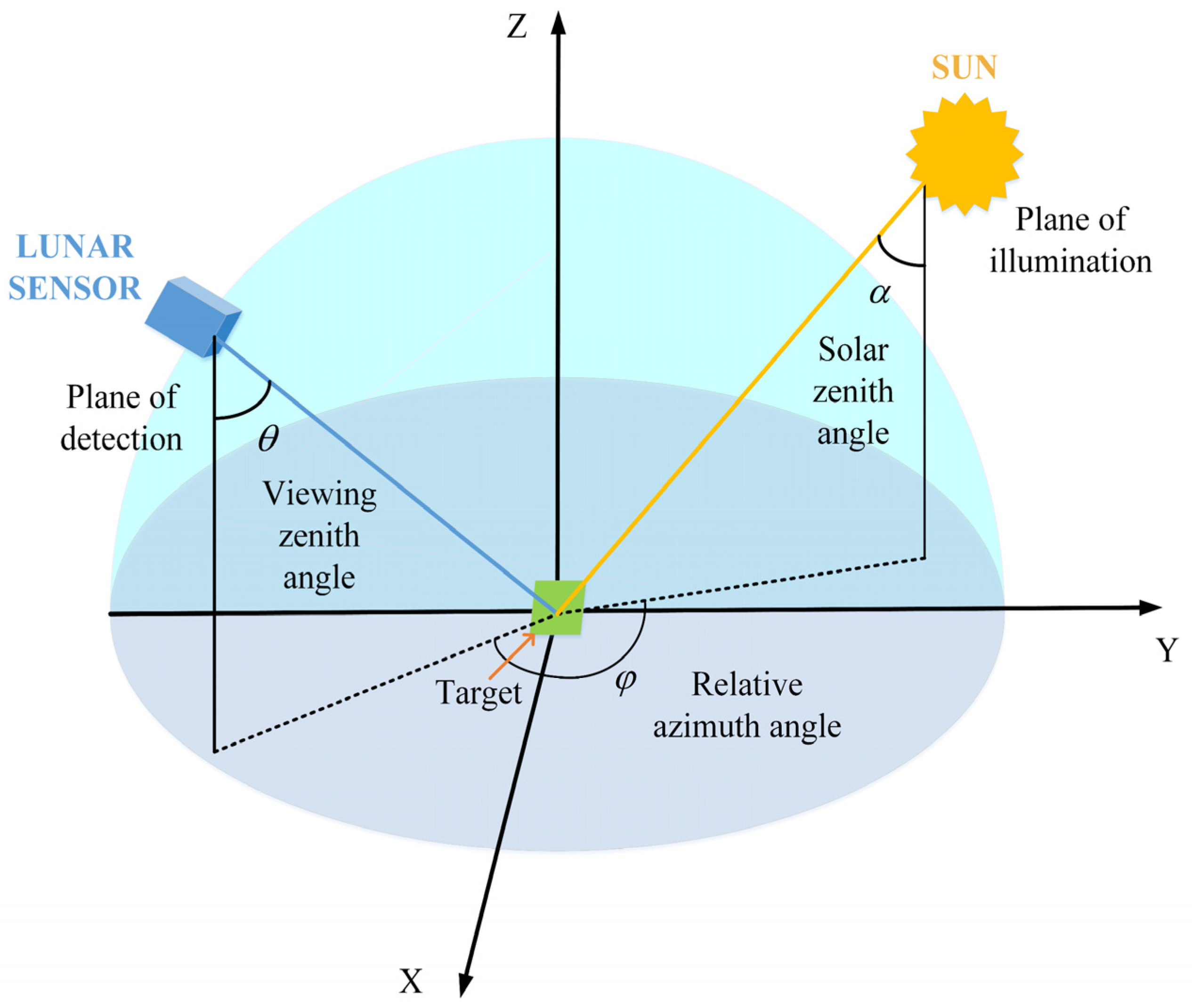
Some scholars have initially carried out pioneering research on the characteristics of angular sampling for a Moon-based platform. Guo et al. [35] and Sui et al. [36] adopted four types of observation angular parameters, that is, the viewing zenith angle, solar zenith angle, viewing azimuth angle, and solar azimuth angle, to describe light incident from the Sun and reflected from surface features. In contrast, Ye et al. [37] reduced the four angular parameters to three parameters by introducing the relative azimuth angle, which is the difference between the viewing and solar azimuth angles. Compared with the four parameters, the relative azimuth angles of the three parameters can be used to directly describe the relative positions of a Moon-based sensor, the Sun, and the observed point. However, few studies have focused on the effect of time sampling interval on the angular combination richness. Ideally, a Moon-based sensor would observe the Earth and collect the angular sampling data continuously. However, in fact, the sensor observes the Earth at a certain time sampling interval. The selection of time sampling intervals will greatly affect the sampling of observations and thus the richness of angular combination. A large time sampling interval will result in the lack of effective angular combination coverage, whereas a small time sampling interval will lead to redundancy in the angular sampling. Furthermore, the effect of the time sampling interval on the angular combination differs for different observed points. Therefore, it is necessary to study the effect of the time sampling interval on the angular combination characteristics for Moon-based Earth observations with respect to different observed points.

The aims of this study were to explore the angular combination characteristics of a Moon-based platform and the effect of time sampling interval for different observed points. We derived an analytical equation for the observational angles from the orbital elements of the Moon and Sun. We also proposed an angular combination number index (ACNI), which can be used to characterize the performance of the angular combination. Finally, the effects of the time sampling interval for different observed points are revealed.

2. Theoretical Analysis of Moon-Based Earth Observational Angles

The aim of this study was to analyze the angular combination for Moon-based Earth observations based on the analytical expression of lunar and solar orbits. In this section, we first introduce the orbital elements of the Sun and Moon. Subsequently, the three observational angles are defined and calculated according to the solar and lunar nadirs. Finally, the ACNI is proposed to evaluate the performance of the angular combination of the Earth observation platform.

2.1. Orbital Elements

To describe orbital variations for the Sun and Moon, the orbits of the Sun and Moon are described based on orbital elements [38]. Note that the orbital elements are defined using Earth-centered ecliptic coordinates [39].

The solar orbital elements can be simply obtained by assuming unperturbed motion of the Earth around the Sun, which mainly includes five orbital elements [40]. In contrast to the Sun, the lunar orbit is strongly affected by solar and terrestrial perturbations, and thus, six orbital elements are required to describe the complex lunar motion [41]. Therefore, additional parameters are required to calculate perturbations of the lunar orbit. The solar and lunar orbital elements and their parameters are listed in

Table 1. Orbital parameters of the Sun and Moon.

Star/Planet	Orbital Parameters	Symbol
Sun	Semimajor axis	$a_s$
	Eccentricity	$e_s$
	Obliquity of the ecliptic	${\epsilon }_s$
	Mean ecliptic longitude of the perigee	${\mathsf{\Gamma }}_s$
	Mean ecliptic longitude of the Sun	$L_s$
	Mean anomaly of the Sun	$l_s=L_s-{\mathsf{\Gamma }}_s$
Earth	Semimajor axis	$a_m$
	Eccentricity	$e_m$
	Inclination	$i_m$
	Mean ecliptic longitude of the ascending node	${\mathsf{\Omega }}_m$
	Mean ecliptic longitude of the perigee	${\mathsf{\Gamma }}_m$
	Mean ecliptic longitude of the Moon	$L_m$
	Mean anomaly of the Moon	$l_m=L_m-{\mathsf{\Gamma }}_m$
	Mean distance of the Moon from the ascending node	$F_m=L_m-{\mathsf{\Omega }}_m$
	Mean elongation of the Moon	$D=L_m-{\mathrm{L}}_s$

.

2.2. Definition and Calculation of Observational Angles

In the following subsections, the coordinates of the solar and lunar nadirs are deduced based on the orbital elements. Subsequently, three observational angles are defined and calculated according to the solar and lunar nadirs. Finally, an ACNI is proposed to determine the characteristics of the angular combination.

2.2.1. Calculation Method for Lunar and Solar Nadirs

Because the orbital elements of the Sun and Moon are defined in the Earth-centered ecliptic coordinate system, we first calculated the ecliptic latitude and longitude and distances of the Moon and Sun from Earth. We mainly adopted a previously described analytical method for the ecliptic coordinates of the Moon and Sun, which are accurate to about 0.1–1% [38]. The ecliptic longitude ${\lambda }_m$ of the Moon is

$${\lambda }_m=L_m+d{l}_m,$$

(1)

where

$$d{l}_m=2e_{m}sin\left(l_m\right)+\frac{5}{4}{e}_m{}^{2}sin2l_m-{4586}^{″}sin\left(l_m-2D\right)+{2370}^{″}sin\left(2D\right).$$

(2)

The ecliptic latitude ${\beta }_m$ is

$${\beta }_m=i_{m}sin\left(F+d{l}_m+∆F\right)+N,$$

(3)

where

$$∆F={412}^{″}sin\left(2F\right)+541″sin\left(l_s\right),$$

(4)

$$N=-{526}^{″}sin\left(F-2D\right)+{44}^{″}sin\left(l+F-2D\right)-{31}^{″}sin\left(-l+F-2D\right)+\cdots .$$

(5)

The Earth–Moon distance $r_m$ is

$$r_m=a_m(1+\frac{1}{2}{e}_m{}^2-e_{m}cos\left(l_m\right)-\frac{1}{2}{e}_m{}^{2}cos\left(2l_m\right)-3699cos\left(2D-l\right)+\cdots ,$$

(6)

Similarly, the solar ecliptic longitude is

$${\lambda }_s=L_s+d{l}_s,$$

(7)

where

$$d{l}_s=2e_{s}sin\left(l_s\right)+\frac{5}{4}{e}_s{}^{2}sin2l_s.$$

(8)

The Sun–Earth distance is

$$r_s=a_s(1+\frac{1}{2}{e}_s{}^2-e_{s}cos\left(l_s\right)-\frac{1}{2}{e}_s{}^{2}cos\left(2l_s\right)).$$

(9)

The solar ecliptic latitude is zero in the Earth-centered ecliptic coordinate system.

However, for Moon-based Earth observations, the ecliptic coordinates of the Moon and Sun must be converted to equatorial coordinates because the position of the observed point is generally defined in the equatorial coordinate system. The equatorial longitude ${\alpha }_m$ and equatorial latitude ${\kappa }_m$ of the Moon can be deduced from the ecliptic longitude ${\lambda }_m$ and ecliptic latitude ${\beta }_m$.

$$sin\left({\kappa }_m\right)=cos\left({\epsilon }_s\right)sin\left({\beta }_m\right)+sin\left({\epsilon }_s\right)cos\left({\beta }_m\right)sin\left({\lambda }_m\right)$$

(10)

$$cos\left({\alpha }_m\right)=\frac{cos\left({\beta }_m\right)cos\left({\lambda }_m\right)}{cos\left({\delta }_m\right)}$$

(11)

$$sin\left({\alpha }_m\right)=\frac{-sin\left({\beta }_m\right)sin\left({\epsilon }_s\right)+cos\left({\beta }_m\right)cos\left({\epsilon }_s\right)sin\left({\lambda }_m\right)}{cos\left({\delta }_m\right)}$$

(12)

Similarly, by substituting the ecliptic longitude ${\lambda }_m$ and ecliptic latitude ${\beta }_m$ for the ecliptic longitude ${\lambda }_s$ and ecliptic latitude ${\beta }_s$ in Equations (14)–(16), the solar equatorial coordinates can be calculated.

$$sin\left({\kappa }_s\right)=cos\left({\epsilon }_s\right)sin\left({\beta }_s\right)+sin\left({\epsilon }_s\right)cos\left({\beta }_s\right)sin\left({\lambda }_s\right)$$

(13)

$$cos\left({\alpha }_s\right)=\frac{cos\left({\beta }_s\right)cos\left({\lambda }_s\right)}{cos\left({\delta }_s\right)}$$

(14)

$$sin\left({\alpha }_s\right)=\frac{-sin\left({\beta }_s\right)sin\left({\epsilon }_s\right)+cos\left({\beta }_s\right)cos\left({\epsilon }_s\right)sin\left({\lambda }_s\right)}{cos\left({\delta }_s\right)}$$

(15)

2.2.2. Definition and Calculation of Observational Angles

The three observational angles, including the viewing zenith angle, solar zenith angle, and relative azimuth angle, are introduced in the topocentric reference system, as shown in Figure 1. The topocentric reference system refers to the Cartesian reference system, whose origin is the observation point. Its z-axis is perpendicular to the ground, and the fundamental plane is the horizontal plane of the observation point.

Based on the topocentric reference system, the viewing zenith angle refers to the angle from the sensor’s nadir to the line of sight. Similarly, the solar zenith angle refers to the angle from solar nadir to the line of sight of the Sun. The relative azimuth angle is the angle between the line of sight of the Sun and that of a Moon-based platform in the horizontal plane.

To describe the relative positions of the observed point and solar and lunar nadirs, an Earth-centered Earth-fixed spherical coordinate system is introduced based on the topocentric reference system. The Earth-centered Earth-fixed spherical coordinate system refers to a coordinate system in which the position of a point is specified by three numbers: the radial distance of that point from a fixed origin, its polar angle measured from a fixed zenith direction, and the azimuthal angle of its orthogonal projection on a reference plane that passes through the origin and is orthogonal to the zenith, measured from a fixed reference direction on that plane. In the Earth-centered Earth-fixed spherical coordinate system, the position of the Moon can be described as follows:

$$M_{SCS}=\left[\begin{array}{c}{r}_{m}sin\left({\theta }_m\right)cos\left({\phi }_m\right)\\ r_{m}sin\left({\theta }_m\right)sin\left({\phi }_m\right)\\ r_{m}cos\left({\theta }_m\right)\end{array}\right].$$

(16)

The two parameters of the spherical coordinates can be derived based on the equatorial longitude and equatorial latitude. The ${\theta }_m$ can be expressed as follows:

$${\theta }_m={\kappa }_m+\frac{\pi }{2}=\frac{\pi }{2}+arcsin\left(cos\left(\epsilon \right)sin\left({\beta }_m\right)+sin\left(\epsilon \right)sin\left(L_m\right)cos\left({\beta }_m\right)\right)$$

(17)

To calculate ${\phi }_m$, we must introduce the Greenwich sidereal time $S$.

$$\begin{gathered} {\phi }_m=\{\begin{array}{c}{\alpha }_m-S\\ 2\pi +{\alpha }_m-S\end{array} \\ =\{\begin{array}{c}arctan(\frac{-sin\left({\beta }_m\right)sin\left(\epsilon \right)+cos\left({\beta }_m\right)cos\left(\epsilon \right)sin\left(L_m\right)}{cos\left({\beta }_m\right)cos\left(L_m\right)})-S\\ 2\pi +arctan(\frac{-sin\left({\beta }_m\right)sin\left(\epsilon \right)+cos\left({\beta }_m\right)cos\left(\epsilon \right)sin\left(L_m\right)}{cos\left({\beta }_m\right)cos\left(L_m\right)})-S\end{array} \end{gathered}$$

(18)

Similarly, we can calculate the spherical coordinates (${\theta }_s, {\phi }_s$) of the Sun by using Equations (16)–(18) and replacing the equatorial longitude and equatorial latitude. The position of the Sun can then be expressed as follows:

$$S_{SCS}=\left[\begin{array}{c}{r}_{s}sin\left({\theta }_s\right)cos\left({\phi }_s\right)\\ r_{s}sin\left({\theta }_s\right)sin\left({\phi }_s\right)\\ r_{s}cos\left({\theta }_s\right)\end{array}\right].$$

(19)

Given the position of the observed point, its spherical coordinates can also be determined.

$$P_{SCS}=\left[\begin{array}{c}Rsin\left({\theta }_p\right)cos\left({\phi }_p\right)\\ Rsin\left({\theta }_p\right)sin\left({\phi }_p\right)\\ Rcos\left({\theta }_p\right)\end{array}\right],$$

(20)

where R is the radius of Earth.

The spherical coordinates of the lunar and solar nadirs and observed point are (${\theta }_m, {\phi }_m,r_m$), (${\theta }_s, {\phi }_s,r_s$), and (${\theta }_p, {\phi }_p,R$), respectively.

Finally, the three observational angles for the Moon-based Earth observation can be derived from the spherical coordinates of the Moon, Sun, and observed point. The viewing zenith angle ${\delta }_m$ can be expressed as follows:

$$cos\left({\delta }_m\right)=\frac{cos\left({\beta }_m\right)-\frac{R}{r_m}}{\sqrt{1+{\left(\frac{R}{r_m}\right)}^2-2\times \frac{R}{r_m}\times cos\left({\beta }_m\right)}},$$

(21)

where

$$cos\left({\beta }_m\right)=sin\left({\theta }_m\right)sin\left({\theta }_p\right)cos\left({\phi }_m-{\phi }_p\right)+cos\left({\theta }_m\right)cos\left({\theta }_p\right).$$

(22)

Similarly, by replacing ${\theta }_m$ and ${\phi }_m$ in Equations (25) and (26) with ${\theta }_p$ and ${\phi }_p$, the solar zenith angle can be calculated:

$$cos({\delta }_s)=\frac{cos\left({\beta }_s\right)-\frac{R}{r_s}}{\sqrt{1+{\left(\frac{R}{r_s}\right)}^2-2\times \frac{R}{r_s}\times cos\left({\beta }_s\right)}},$$

(23)

where

$$cos\left({\beta }_s\right)=sin\left({\theta }_s\right)sin\left({\theta }_p\right)cos\left({\phi }_s-{\phi }_p\right)+cos\left({\theta }_s\right)cos\left({\theta }_p\right).$$

(24)

The relative azimuth angle $∆\phi$ refers to the difference between the solar and lunar azimuth angles and can be calculated as follows:

$$cos\left(∆\phi \right)=\frac{\overrightarrow{S}·\overrightarrow{M}}{\parallel \overrightarrow{S}\parallel \parallel \overrightarrow{M}\parallel },$$

(25)

where

$$\overrightarrow{S}=\overrightarrow{PS}-\frac{\overrightarrow{PS}·\overrightarrow{P}}{{\parallel \overrightarrow{P}\parallel }^2}\overrightarrow{P}=r_s\left[\begin{array}{c}sin\left({\theta }_p\right)cos\left({\theta }_s\right)-cos\left({\theta }_p\right)sin\left({\theta }_s\right)cos\left({\phi }_s-{\phi }_p\right)\\ sin\left({\theta }_s\right)sin\left({\phi }_s-{\phi }_p\right)\end{array}\right]$$

(26)

$$\overrightarrow{M}=\overrightarrow{PM}-\frac{\overrightarrow{PM}·\overrightarrow{P}}{{\parallel \overrightarrow{P}\parallel }^2}\overrightarrow{P}=r_m\left[\begin{array}{c}sin\left({\theta }_p\right)cos\left({\theta }_m\right)-cos\left({\theta }_p\right)sin\left({\theta }_m\right)cos\left({\phi }_m-{\phi }_p\right)\\ sin\left({\theta }_m\right)sin\left({\phi }_m-{\phi }_p\right)\end{array}\right]$$

(27)

$\overrightarrow{S}$ and $\overrightarrow{M}$ are the two-dimensional vectors projected on the XY plane of the line-of-sight vector from the sensor and Sun, respectively.

In summary, the observational angles are mainly determined based on the relative positions of the observed point and lunar and solar nadirs, which are affected by the orbital elements of the Moon and Sun.

2.2.3. Observational Angular Combination Performance Index

The purpose of this study was to evaluate the effect of the time sampling interval on the characteristics of the angular combination. Therefore, we must define several parameters to describe the characteristics of the angular combination. In this subsection, we introduce the definition and calculation method of the ACNI proposed in this paper.

The ACNI refers to the maximum coverage of the three-angle combination range over a specific time sampling interval during the observation period. When the angular combination is completely covered, the ACNI reaches a maximum value; conversely, the ACNI reaches a minimum value. Note that the ACNI has no units. In practical applications, we first must discretize the range of the three-angle combination to facilitate the calculation. The required parameters are the size and number of discrete bins for the three angles.

The calculation of the ACNI consists of three main steps. In the first step, the observation period and time sampling interval are defined. In the second step, the ranges of the three angles are discretized based on the input parameters. It is assumed that the viewing zenith angle is divided into p angular bins, solar zenith angle has q angular bins, and relative azimuth angle has m angular bins. In the last step, all observation samplings are traversed to calculate the maximum coverage. First, we can use Equations (21)–(27) to calculate the three observational angles for each observation. Subsequently, we can identify the corresponding angle bin and record it in a three-dimensional Boolean matrix R:

$$R_{ijk}=\{\begin{array}{c}1, {\delta }_{ijk}>0\\ 0,{\delta }_{ijk}\le 0\end{array},$$

(28)

where $R_{ijk}$ reflects if the ith viewing zenith angle bin, jth solar zenith angle bin, and kth relative azimuth angle bin are covered. If the value is 1, this angle bin is covered; otherwise, it is uncovered. The parameter ${\delta }_{ijk}$ refers to the angular sampling times corresponding to the ith viewing zenith angle bin, jth solar zenith angle bin, and kth relative azimuth angle bin.

Finally, all p viewing zenith angle bins, q solar zenith angle bins, and m relative azimuth angle bins are traversed to calculate the ACNI.

$$\cup ={\displaystyle \sum }_{i=1}^p{\displaystyle \sum }_{j=1}^q{\displaystyle \sum }_{k=1}^m{R}_{ijk}$$

(29)

The maximum value of ACNI is $p\times q\times m,$ and the minimum value is zero. Based on ACNI, we can calculate the angular coverage ratio using the following equation:

$$\gamma =\frac{\cup }{p\times q\times m},$$

(30)

where $\gamma$ is the ratio of the ACNI, which has a maximum value of 1 and a minimum value of 0. Note that this term is also unitless.

3. Results

The theoretical framework for analyzing the angular combination of observed points was introduced in Section 2. In this section, we mainly describe how the experiments were conducted to reveal the angular combination characteristics and effects of the time sampling interval. We first compare the results derived from our proposed method with planetary ephemerides. Subsequently, the angular combination distributions and their variations over different time sampling intervals are presented for different observed points. Finally, the effects of the time sampling intervals by using the angular combination performance index are analyzed in detail. Note that the coordinated universal time (UTC) is adopted.

3.1. Validation

To validate the analytic coordinates of the Sun and Moon, our results were compared with planetary ephemerides. As mentioned in Section 1, the DE is one of the main streams of planetary ephemerides. The DE430 was selected because of the improvements based on the use of additional lunar laser ranging data and improved lunar gravity field for the lunar orbit and attitude. For the lunar position, the coordinates based on DE 430 were tabulated as the origin at the Earth barycenter, that is, the geocentric celestial reference system. The lunar attitude is expressed by three Euler angles based on the DE 430 [24].

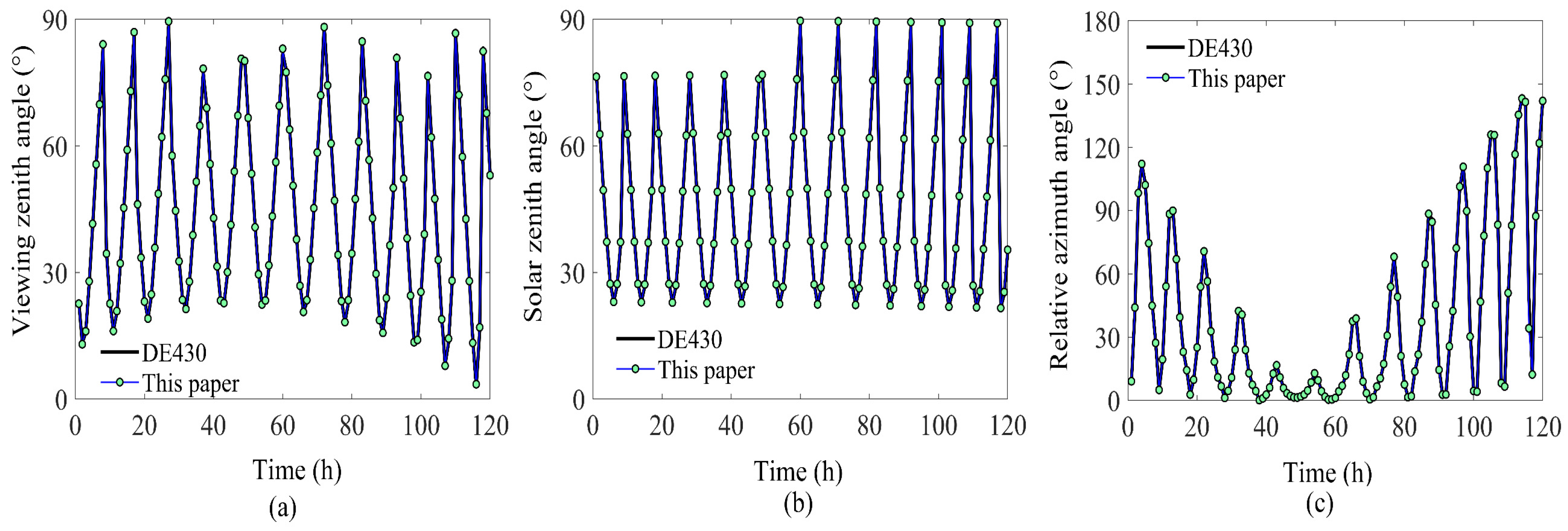
We assumed that the sensor was equipped at (0°, 0°) on the Moon and the observed point was located at (0°, 0°) on the Earth. Notice that the mean orbital elements of the Sun and Moon are adopted with respect to the Earth and the ecliptic for decades around the year 2000 [38]. Figure 2 shows comparisons between the results derived from DE430 and our method during one orbital period. Note that the orbital period refers to the period it takes the Moon to complete one revolution relative to the Sun (a synodic month). Considering the relative azimuth angle is defined as the angle between the Moon and Sun, the x-axis represents the time when the observed point was simultaneously visible by the Moon and Sun. The y-axis represents the results for the three observational angles. The blue and orange lines represent the angles calculated using DE430 and our proposed method, respectively. The results derived from our proposed method almost coincide with those obtained from DE430, within 1° of error, verifying the correctness and validity of our analytical method.

3.2. Variation Analysis of the Angular Combination Distribution

The angular combination distribution refers to the coverage of the three observational angles. For an Earth observation platform, the angular combination distribution characterizes the capability of its angular sampling. For a Moon-based platform, the angular combination distribution differs at different observation points because of the orbital characteristics of the Moon and Sun. The orbits of the Moon and Sun can be parameterized as the distance from the Earth and the position of nadirs. It can be inferred from Equations (21)–(27) that the distance does not significantly influence the zenith angles and relative azimuth angle. Hence, the movement of lunar and solar nadirs are the primary factors affecting the angular combination distribution. Actually, neither the Sun nor the Moon has a fixed orbital inclination. As the Earth’s rotational axis is inclined about 23°27′ with respect to the ecliptic plane, the Sun’s nadir varies between the 23°27′ N and 23°27′ S over one year. The Moon’s inclination also changes. As the Moon is orbiting the Earth, the plane of the Moon’s orbit is tilted (around 5°9′) with respect to the ecliptic plane. Thus, the lunar nadir moves between the southern and northern hemispheres for one orbital period. It is clear that the Moon’s maximum and minimum declination vary because the mean ecliptic longitude of the ascending node continuously recedes westward along the ecliptic. It recedes about 19° westward every year over an 18.6-year period. Consequently, when the mean ecliptic longitude of the ascending node is 0°, the ascending node coincides with the vernal equinox, and thus the obliquity of the ecliptic reaches a maximum. In contrast, when the mean ecliptic longitude of the ascending node is 180°, the descending node and vernal equinox coincide, and the obliquity of the ecliptic reaches a minimum. Therefore, the extreme value of the Moon’s nadir varies roughly from about 18° to 28° over an 18.6-year period. Variations in the Moon’s and Sun’s nadirs lead to differences in the angular combination distribution for different observed points. In general, as the Moon’s and Sun’s nadirs mainly move within the mid–low latitude zone, the viewing and solar zenith angle of observed points in this region can reach a maximum of 90° and thus range from 0° to 90°. For the solar zenith angle, its minimum varies with the seasons because of the movement regularity of the Sun’s nadir, and the maximum difference is around 23°. For the viewing zenith angle, the difference of its maximum can reach 10° under the two extreme cases of 0° and 180° for mean ecliptic longitude of ascending node. The relative azimuth angle is defined only when the observed points can be visible by the Moon and Sun simultaneously. Thus, it is mainly affected by the Moon phase angle. The moon phase refers to the part of the Moon that is illuminated by the Sun and can also be seen on the Earth. It represents the relative position of the Moon, Sun, and Earth. Specifically, it mainly affects the difference between the longitude of the Sun’s and Moon’s nadir, and the period of the moon phase angle is a synodic month.

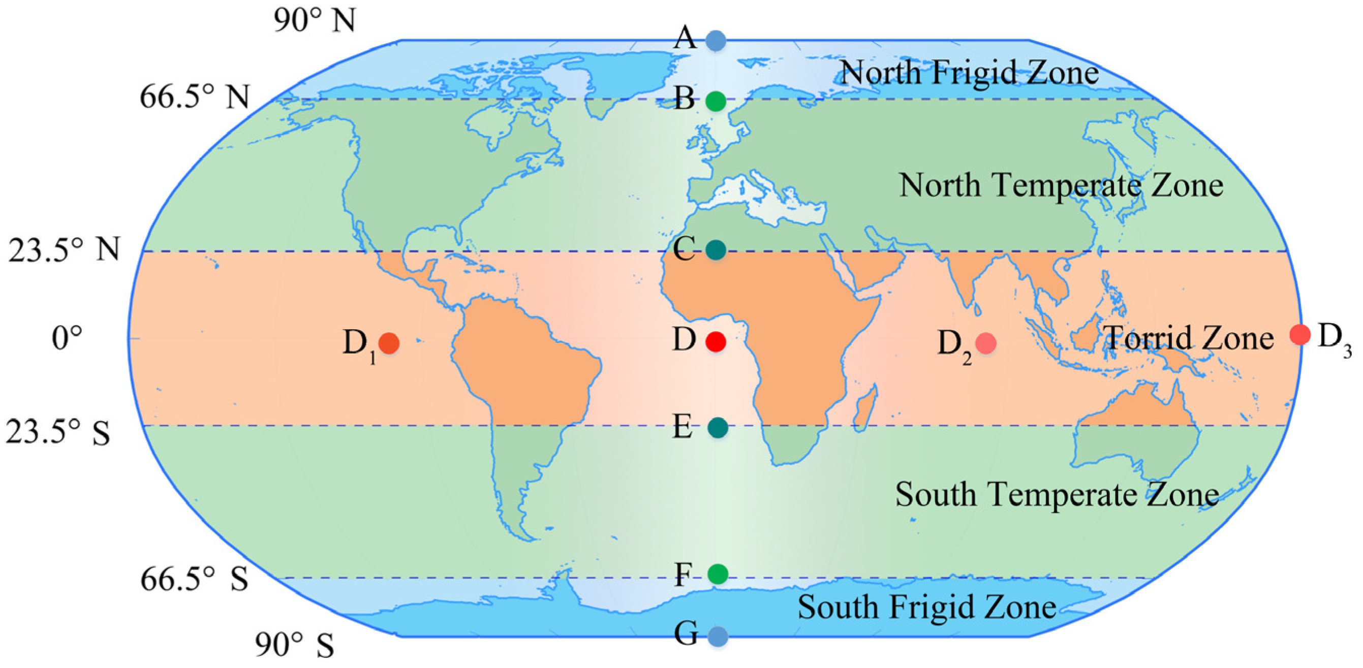
To reveal differences in the distribution of the angular combination for different observed points, we compared the latitudinal and longitudinal variations for selected points. As shown in Figure 3, ten observed points were selected at different latitudes and longitudes for experiments. Points A–G are on the Earth’s central meridian along the longitude, and Points D, D₁, D₂, and D₃ are on Earth’s equator along the latitude. Note that the observation period of the experiments in this study was set to 18.6 years according to the periodicity of the lunar nadir. 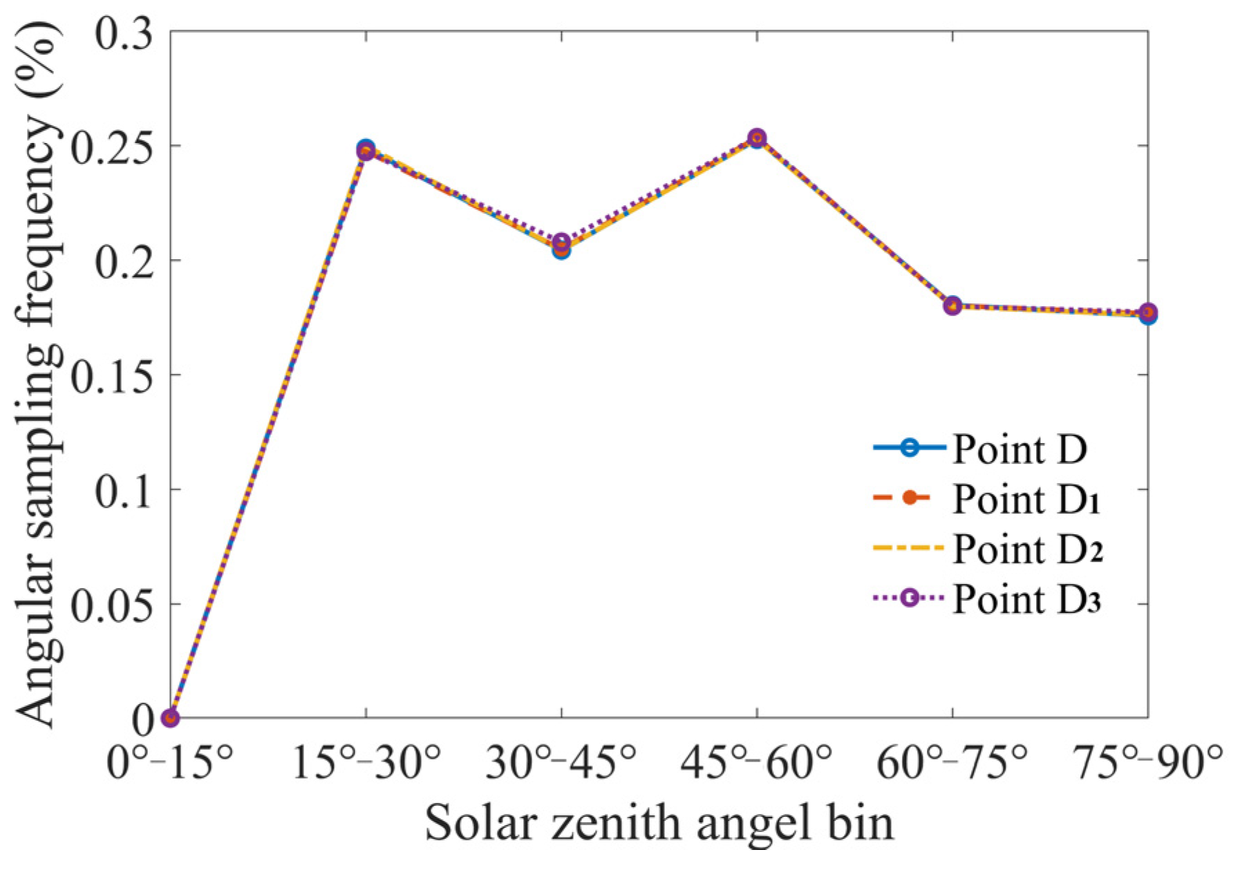Figure 4 shows the 18.6-yearly latitudinal angular sampling frequency for different longitudes. We divided the solar zenith angle with 15° interval and calculated the angular sampling frequency in each solar zenith angle bin. The results show that all the D points have the same angular frequency distribution. Therefore, in general, the longitude of the observed point has no significant effect on the angular combination distribution over a period of 18.6 years. 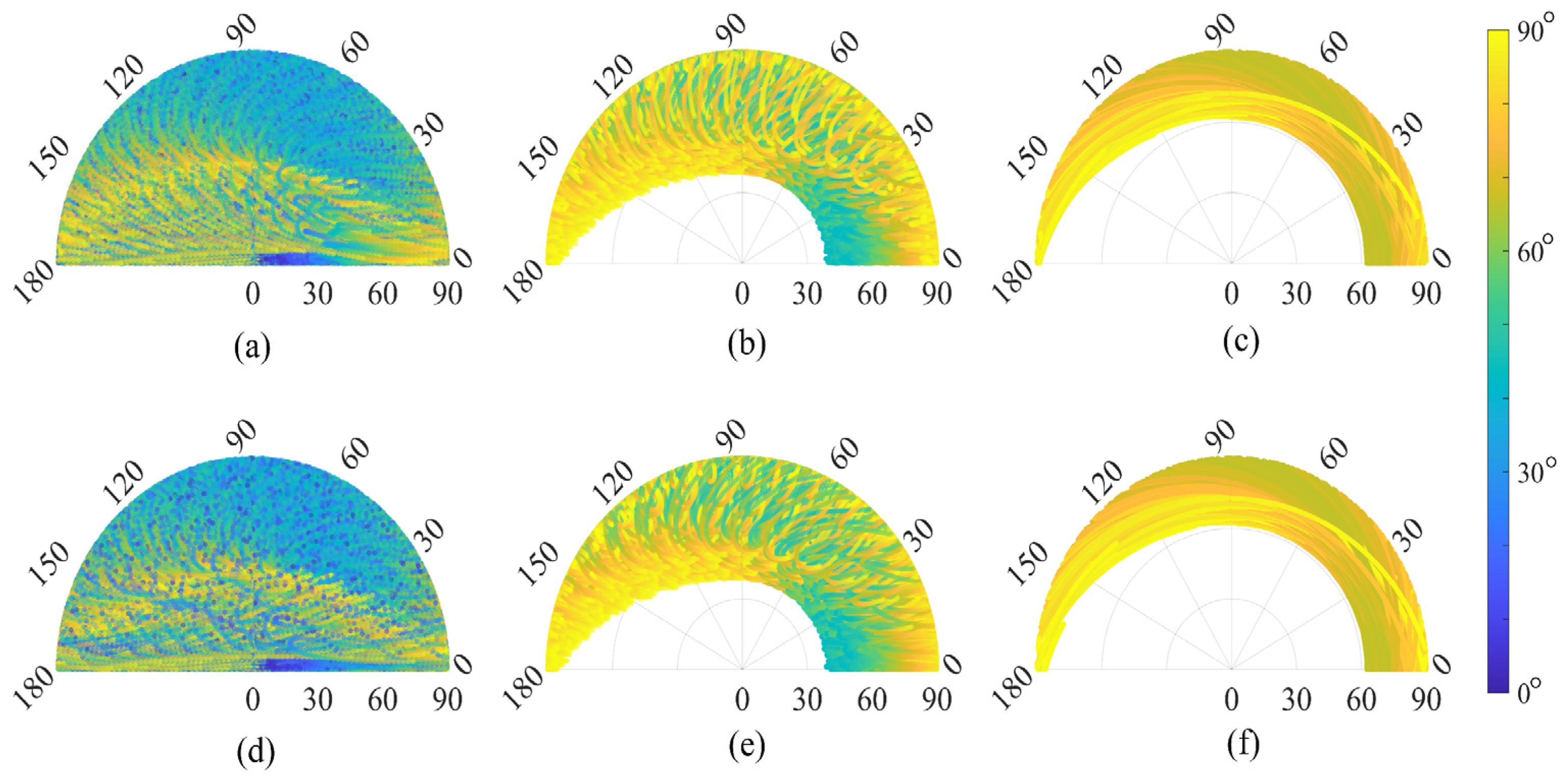Figure 5 shows the distributions of the angular combination at different latitudes. The distributions of the longitudinal angular combination differ at different latitudes because both the Moon’s and Sun’s nadir move along the latitude direction. In addition, a slight difference was observed between the observed points, which are symmetrical around the equator. For example, Point C is similar to Point E with respect to the pattern of angular distribution. As expected, compared with the observed points in the high latitude zone, the distribution of the angular combination is more abundant for the observed points in the mid–low latitude zone. This further advances our understanding of the angular characteristics for Moon-based Earth observations. To exploit the effect of the time sampling interval, we further analyzed the variations in the distribution of the angular combination over different time sampling intervals for different observed points. 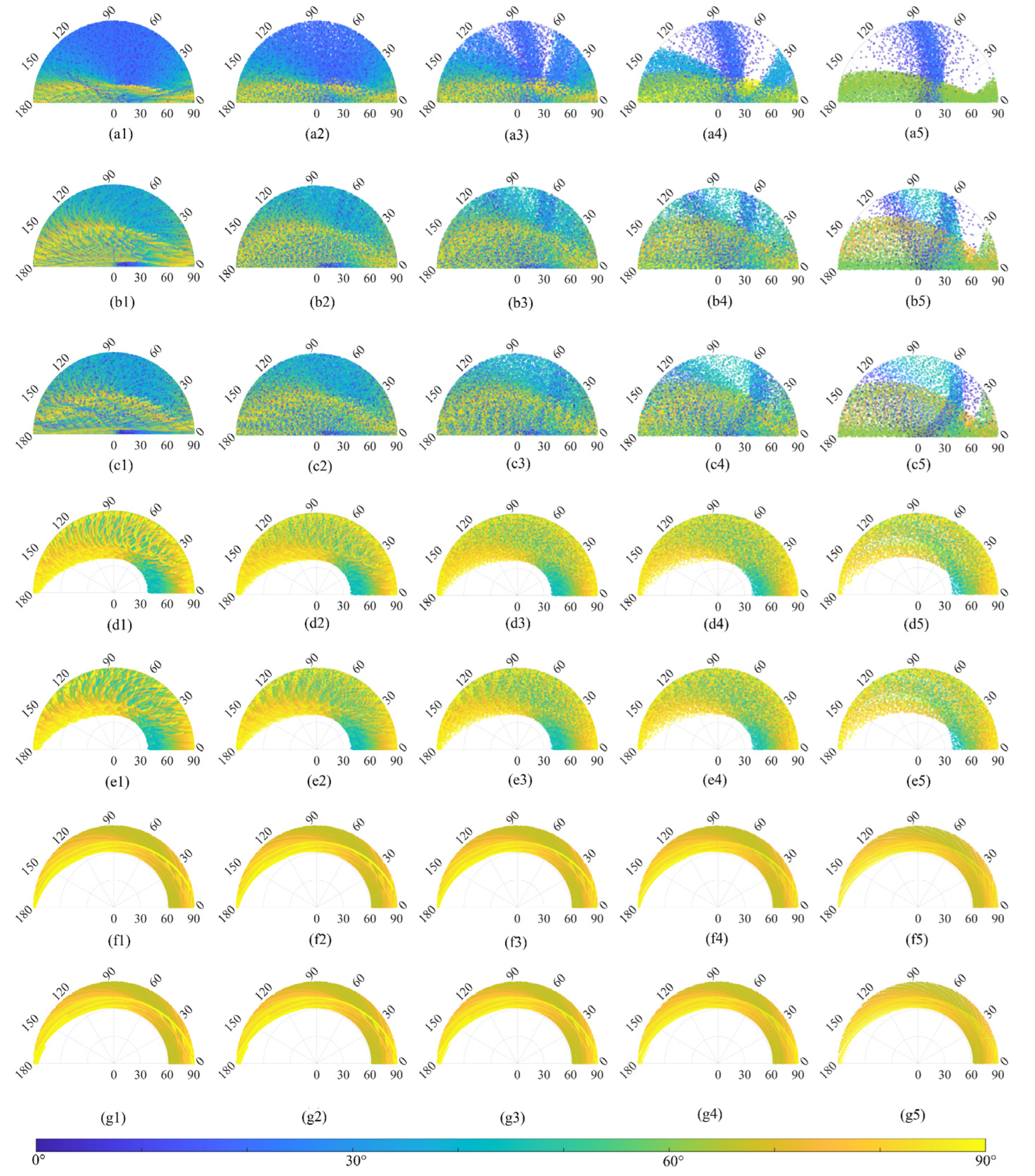Figure 6 shows the variations in the distribution of the angular combination over time sampling intervals of 10 min, 30 min, 1 h, 2 h, and 4 h. The results show that the time sampling interval significantly affects the angular combination distribution. More specifically, for observed points in the mid–low latitude zone, an increase in the time sampling interval results in a larger loss of coverage for certain angular combinations. Thus, the sensitivities of different angular combinations to the time sampling interval differ. In conclusion, the latitude of the observed point affects the angular combination distribution, and an increase in the time interval will result in the loss of certain angular combinations.

3.3. Effect of the Time Sampling Interval on the Angular Combination

As described in Section 3.2, we found that the angular distributions show differences for different observed points, which will be significantly affected by the selection of time sampling interval. This raises the question of the difference in the angular coverage ratio between different observed points and how much an increased time sampling interval will affect the diversity of angular combinations. To answer these questions, we propose the ACNI and its ratio to characterize and quantify the performance of angular combination. One critical step is to discretize the combination of angles according to the bin size. When the ratio of index is a maximum of 1, the sensor can cover all angular combination bins. In contrast, when the ratio is smaller, the sensor’s angular samplings are insufficient. Its minimum is 0, indicating that the observed points cannot be observed. The experiments were conducted assuming the sensor was at (0°, 0°) on the lunar surface, and the observation period was set as 18.6 years to remove the effect of the observation period. Considering the angular resolution of the angular distribution model for the top-of-atmosphere radiative flux calculation, the angular resolution was selected to be 5° [6]. Accordingly, there are 18 bins for the viewing and solar zenith angles and 36 bins for the relative azimuth angle. That means, in Equation (29), the values of p, q, and m are 18, 18, and 36, respectively. Thus, the total number of angular combinations for the three observational angles is 11,664.

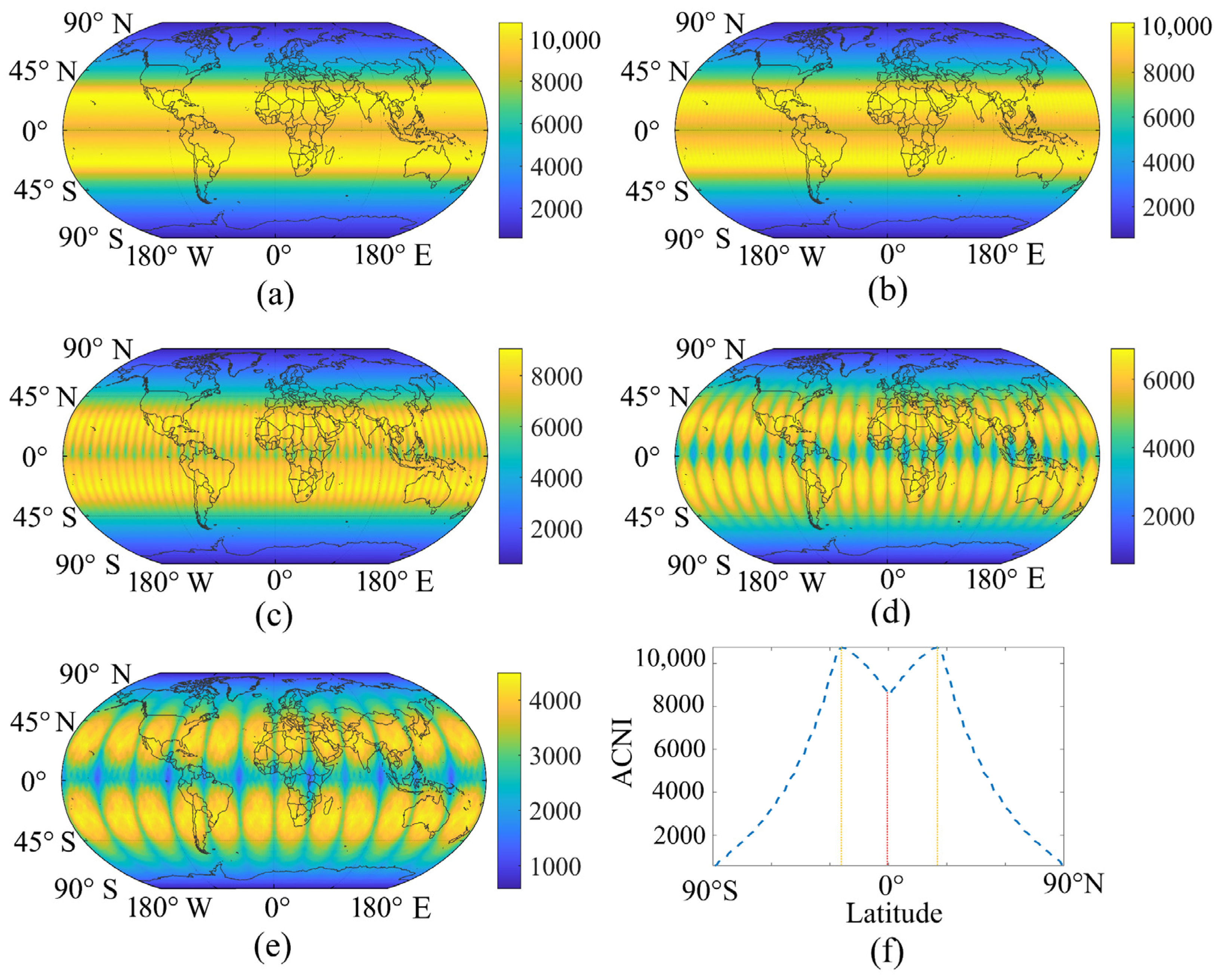
Figure 7 shows the 18.6-yearly variations over time sampling intervals of 10 min, 30 min, 1 h, 2 h, and 4 h. The values in the Figure 7 and Figure 8 represent the numbers of angular combinations and have no physical unit. As expected, the results in Figure 6a appear to be symmetrical around the Earth’s equator and are consistent at the same latitude. This further supports that the angular combination is significantly affected by the latitude of the observed point, whereas the longitude has no significant influence. The angular combination is relatively abundant in the region between 30° N and 30° S, and the values of ACNI vary from approximately 9000 to 10,800, as shown in Figure 7a. Thus, more than 78% of the angular combination can be covered by a Moon-based sensor. The index of observed points in the high latitude zone, however, ranges roughly from 2000 to 8000. The observed points in the polar regions have the smallest index value (approximately 2000), regardless of the time sampling interval, although they have the longest continuous observation duration. Therefore, the values of the index clearly vary with the latitudes of observed points, as shown in Figure 7f. The x-axis represents the latitude of the observed points, and the y-axis represents the value of this index. The two yellow lines correspond to these two latitude lines with the most abundant angular combination sampling, and the red line represents the latitude of the equator index. The angular coverage ratio of the observed point at the equator is 15% lower than the case of these two latitudes lines. Another important issue is the effect of the time sampling interval. 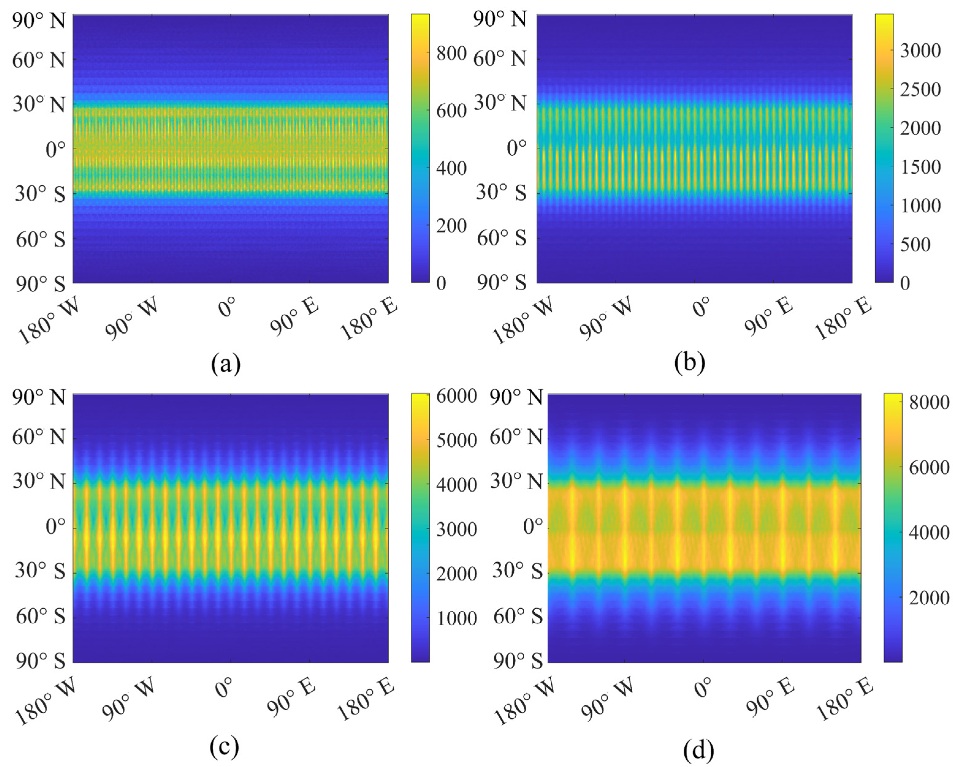Based on a comparison of the four subfigures shown in Figure 6, an increase in the time sampling interval will lead to the loss of consistency at the same latitude, and the pattern in the mid–low latitude zone gradually presents as a scattered petal shape. Because of the apparent “gaps,” the results no longer appear horizontally striped. Interestingly, the number of gaps and time sampling interval are negatively linearly correlated. When the time sampling interval was 1, 2, and 4 h, 48, 24, and 12 gaps were presented, respectively. This is because a larger time sampling interval means more sparse observations. As the Moon orbits the Earth, when the time sampling interval increases, the samples are decreased along the longitude uniformly. Consequently, gaps are presented with increased time sampling intervals, and a larger time sampling interval leads to a larger gap. To evaluate the difference between different time sampling intervals, we calculated a difference map during an 18.6-year period, as shown in Figure 8. The results over a time sampling interval of 10 min were used as the reference map. The results show that the difference of angular coverage presents regular variations and time sampling interval has a larger effect on the angular combination of the observed points in the mid–low latitude zones and latitude ranges from around 30° N to 30° S. 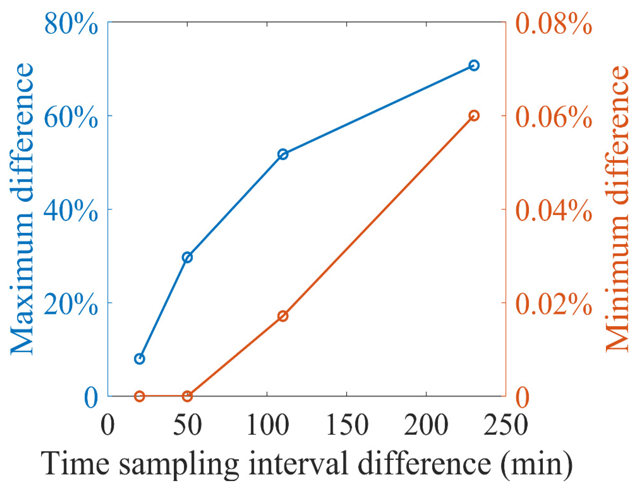To express the trend more clearly, Figure 9 shows the maximum and minimum variations of the ACNI ratio difference with increasing time sampling interval differences. The x-axis represents the difference between the time sampling interval and 10 min. The blue line represents the maximum difference of the index, and the orange line is the minimum difference. When the time sampling interval increases from 10 min to 2 h, the maximum loss reaches 50% in the mid–low latitude zone, whereas the minimum loss in the high latitude zone is less than 0.02%. When the time sampling interval increases to 4 h, the maximum loss rate reaches 70%, and the minimum loss rate is about 0.06%.

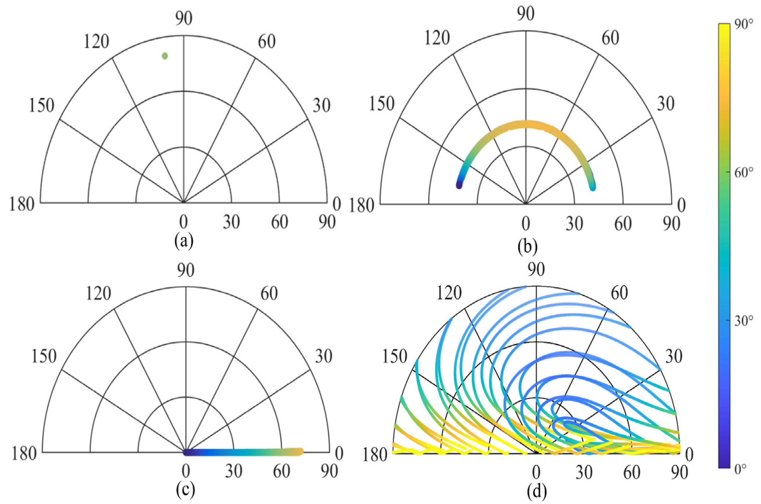
As mentioned in the Section 1, the angular combination characteristics of the Moon-based platform differ from the traditional satellites. Figure 10 shows the angular sampling of LEO, GEO, L1 satellites, and Moon-based platform over an orbital period. The time sampling interval is 1 min, and the Earth location is assumed at (0°, 0°). The results show that the LEO satellite samples sparsely due to the limitation of orbital altitude and field of view. The solar zenith angles of the GEO/L1 satellites can almost cover from 0° to 90°. They mainly lack the corresponding view zenith angle (GEO satellite) or relative azimuth angle (L1 satellite) sampling. To quantify this difference, we further simulated the angular sampling of hemispheric-scale observation platforms from global observed points over 18.6 years based on ACNI. To eliminate the effect of time sampling interval, it is set to 1 h in all cases. We compared all observed points and calculated the largest and smallest ACNI values and their ratios. The comparison results are tabulated in

Table 2. A comparison table of the angular characteristics of each observation platform.

Index	Statistic	GEO Satellite	L1 Satellite	Moon-Based Platform
ACNI	Maximum	372	67	9063
	Minimum	0	9	596
ACNI ratio	Maximum	3.19%	0.57%	77.70%
	Minimum	0.00%	0.00%	5.11%

. For the GEO satellite, limited by the fixed viewing direction, its maximum ACNI value is only 372, and the maximum ratio is 3.19%. Because it always “stares” at the same side of the Earth in a fixed direction, some observed points cannot be observed, and thus the minimum ACNI is zero. For the special L1 satellite, because of its extremely high orbital altitude, it can achieve global coverage. Due to its special position of the Sun–Earth L1 point, the solar direction and viewing direction of the observed point, however, almost coincide. Consequently, the ACNI maximum is 67, and the ACNI minimum is 9. For a Moon-based platform, its maximum ACNI is 9063, which accounts for 77.7%. The minimum ACNI is 596, accounting for 5.11%. The angular sampling results benefit from its variable orbital inclination and altitude. In this sense, lunar observations can provide unique and continuous angular sampling coincident with other satellite observations.

In general, the ACNI can be used to effectively characterize variations in the angular combination. Through experiments, we can determine the magnitude of the difference of the angular combination and the extent of the impact of the time sampling interval with respect to different observed points. We found that the two highest ACNI lines correspond to two latitude lines, which indicate the positions of the observed points with the most abundant angular combination. The angular coverage ratio of observed points at the equator is 15% lower than the case of these two latitudes lines. The time sampling interval has different effects on different observed points, with a greater effect on the observed points in the mid–low latitude zone. When the time sampling interval increases from 10 min to 2 h, the maximum loss of angular combinations reaches 50% for the observed points in the mid–low latitude zone, whereas the minimum loss in the high latitude zone is less than 0.02%. These results provide guidance for selecting time sampling intervals for Moon-based Earth observations with respect to the angular combination performance.

4. Discussion

Different from traditional artificial satellites, a Moon-based platform is equipped with Earth’s natural satellite. Our study mainly focuses on the characteristics of the angular combination of Moon-based Earth observations. The observational angles are mainly affected by the positions of the observed point, solar, and lunar nadirs. Thus, we directly derived the observational angles from the analytical orbits of the Moon and Sun. Based on the observational angular model, an ACNI was proposed to characterize the angular performance. Furthermore, we analyzed the effect of the observed point’s position and time sampling interval on the angular combination, which is beneficial for selecting observed points with optimal observation angle combinations and an appropriate time sampling interval. When the region of interest is at mid–low latitudes, a smaller sampling interval should be selected to avoid loss of the angular combination coverage. In contrast, if the region is at high latitude, a larger time sampling interval can minimize redundant observations while ensuring minimal angular combination coverage losses.

The angular sampling characteristic of an observation platform depends on its observation geometry. As shown in Table 2, the GEO satellite has continuous solar angles and constant viewing angles. On the contrary, the L1 satellite has continuous viewing angles and a constant relative azimuth angle. The Moon, as the sole natural satellite, always faces the Earth on the same side because of the tidal lock. As the Earth rotates, a Moon-based sensor can obtain varied and continuous observational angles on a hemispheric-scale view (Figure 4, Figure 5 and Figure 6). Additionally, the Moon’s orbital inclination and altitude are variable. Therefore, a Moon-based sensor can obtain abundant angular combination sampling. In this sense, a Moon-based platform has continuous viewing and solar observational angles, which can complement angular sampling observations from existing satellites.

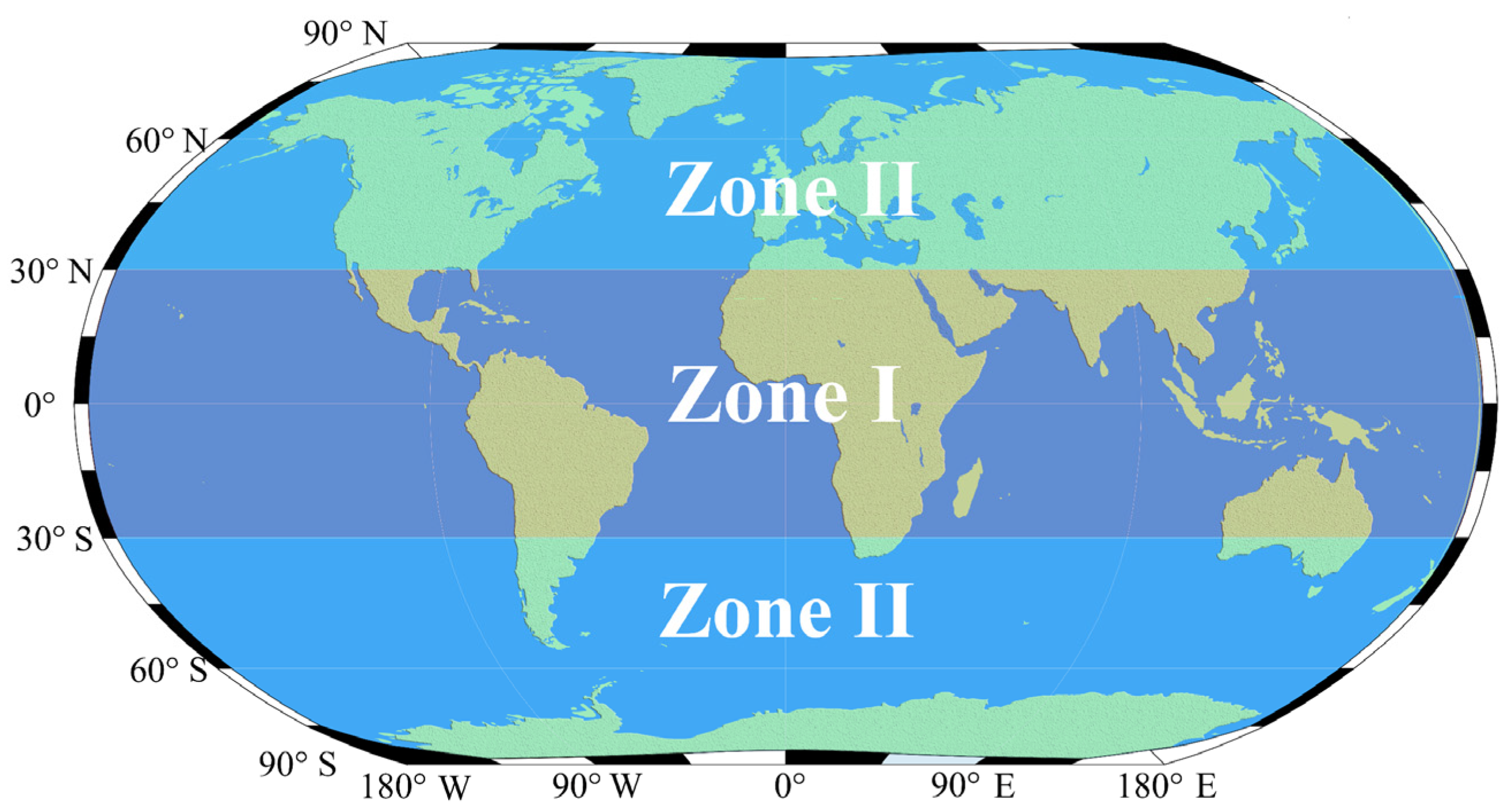
As can be inferred from the results, the time sampling interval has a different effect on the angular combination for different observed points. From Figure 8, the difference maps between different time sampling intervals show regular variations. It is found that the time sampling interval significantly affects the angular combination characteristics for the observed points in the mid–low latitude zone. The angular combination of observed points in the high latitude zone is less sensitive to time sampling intervals. Therefore, the Earth’s surface can be divided into two major zones, as shown in Figure 11. Zone I is in the mid–low latitude zone, and its latitude varies from 30° S to 30° N. For the observed point in Zone I, the angular combination is sensitive, however, to the variety of the time sampling interval. The Zone II consists of two parts, which are between 30° N and 90° N, or 30° S and 90° S. The observed points in these latitude zones are not sensitive to the variations of the time sampling interval.

5. Conclusions

We analyzed the effects of the time sampling interval on the angular combination characteristics of Moon-based Earth observations. A theoretical model was deduced for the three observational angles based on the analytical orbits of the Moon and Sun. Subsequently, an ACNI was proposed to characterize the angular performance of the Moon-based platform. Furthermore, the effects of different positions of observed points on the angular distribution were determined. Finally, the effect of time sampling interval on the angular combination was analyzed based on variations in the ACNI. The results show that the ACNI can be used to characterize the variation in the angular combination of the Earth observation platform. We found that the time sampling interval has different effects on the angle combination for the different observed points and mainly affects the observed points in mid–low latitude zones. According to the sensitivity to the time sampling interval, the Earth’s surface can be divided into two zones. When the time sampling interval increases from 10 min to 2 h, the maximum loss of the ACNI is more than 50% for the observed points in the mid–low latitude zone; when the time sampling interval increases to 4 h, the loss rate reaches 70%.

References

1. Yu, C.; Yasushi, M.; Tamio, T. An empirical anisotropy correction model for estimating land surface albedo for radiation budget studies. Remote Sens. Environ. 2009, 113, 24–39. [Google Scholar]
2. Bacour, C.; Bréon, F.M. Variability of biome reflectance directional signatures as seen by POLDER. Remote Sens. Environ. 2005, 98, 80–95. [Google Scholar] [CrossRef]
3. Henderson-Sellers, A.; Wilson, M.F. Surface albedo data for climatic modeling. Rev. Geophys. 1983, 21, 1743–1778. [Google Scholar] [CrossRef]
4. Loeb, N.G.; Wielicki, B.A.; Barkstrom, B.R.; Smith, G.L.; Wong, T. Top of atmosphere albedo estimation from angular distribution models using scene identification from satellite cloud property retrievals. J. Clim. 2000, 13, 1269–1285. [Google Scholar] [CrossRef] [Green Version]
5. Wielicki, B.A.; Barkstrom, B.R.; Harrison, E.F.; Lee, R.B.; Smith, G.L.; Cooper, J.E. Clouds and the Earth’s Radiant Energy System (CERES): An Earth Observing System Experiment. Bull. Am. Meteorol. Soc. 1998, 36, 1127–1141. [Google Scholar] [CrossRef] [Green Version]
6. Loeb, N.G.; Doelling, D.R.; Wang, H.; Su, W.; Nguyen, C.; Corbett, J.G.; Liang, L.; Mitrescu, C.; Rose, F.G.; Kato, S. Clouds and the Earth’S Radiant Energy System (CERES) Energy Balanced and Filled (EBAF) top-of-atmosphere (TOA) edition-4.0 data product. J. Clim. 2017, 31, 895–918. [Google Scholar] [CrossRef]
7. Loeb, N.G.; Wielicki, B.A.; Doelling, D.R.; Smith, G.L.; Keyes, D.F.; Kato, S.; Manalo-Smith, N.; Wong, T. Toward Optimal Closure of the Earth’s Top-of-Atmosphere Radiation Budget. J. Clim. 2009, 22, 748–766. [Google Scholar] [CrossRef] [Green Version]
8. Guo, H.; Fu, W.; Liu, G. Earth Observation Technologies and Scientific Satellites for Global Change, Corrected, 1st ed.; Springer Nature: Singapore, 2019; pp. 31–49. [Google Scholar]
9. Deng, Y.; Guo, H.; Liu, G.; Ye, H.; Huang, J.; Dong, R. Comparisons of Observational Angles between Moon-based Platform and Artificial Satellites. In Proceedings of the IEEE International Geoscience and Remote Sensing Symposium, Brussels, Belgium, 11–16 July 2021. [Google Scholar]
10. Diner, D.J.; Braswell, B.H.; Davies, R. The value of multiangle measurements for retrieving structurally and radiatively consistent properties of clouds, aerosols, and surfaces. Remote Sens. Environ. 2005, 97, 495–518. [Google Scholar] [CrossRef]
11. Govaerts, Y.M.; Lattanzio, A.; Taberner, M. Generating global surface albedo products from multiple geostationary satellites. Remote Sens. Environ. 2008, 112, 2804–2816. [Google Scholar] [CrossRef]
12. Li, X.; Yang, L.; Su, X.; Hu, Z.; Chen, F. A correction method for thermal deformation positioning error of geostationary optical payloads. IEEE Trans. Geos. Remote Sens. 2019, 57, 7986–7994. [Google Scholar] [CrossRef]
13. Song, W.; Knyazikhin, Y.; Wen, G.; Marshak, A. Implications of Whole-Disc DSCOVR EPIC Spectral Observations for Estimating Earth’s Spectral Reflectivity Based on Low-Earth-Orbiting and Geostationary Observations. Remote Sens. 2018, 10, 1594. [Google Scholar] [CrossRef] [Green Version]
14. Selva, D.; Krejci, D. A survey and assessment of the capabilities of CubeSats for Earth Observations. Acta Astron. 2012, 74, 50–68. [Google Scholar] [CrossRef]
15. Rose, T.S.; Rowen, D.W.; LaLumondiere, S. Optical communications downlink from a 1.5 U CubeSat: OCSD program. In Proceedings of the International Conference on Space Optics—ICSO 2018, Chania, Greece, 9–12 October 2018. [Google Scholar]
16. Cullingworth, C.; Muller, J.-P. Contemporaneous Monitoring of the Whole Dynamic Earth System from Space, Part I: System Simulation Study Using GEO and Molniya Orbits. Remote Sens. 2021, 13, 878. [Google Scholar] [CrossRef]
17. Wulder, M.A.; Hilker, T.; White, J. Virtual constellations for global terrestrial monitoring. Remote Sens. Environ. 2015, 170, 62–76. [Google Scholar] [CrossRef] [Green Version]
18. Guo, H. Earth System Observation from Space: From Scientific Satellite to Moon-based Platform. J. Remote Sens. 2016, 5, 716–723. [Google Scholar]
19. Pallé, E.; Goode, P.R. The lunar terrestrial observatory: Observing the earth using photometers on the moon’s surface. Adv. Space Res. 2009, 43, 1083–1089. [Google Scholar] [CrossRef]
20. Carruthers, G.R. Apollo 16 far-Ultraviolet Camera/Spectrograph: Instrument and Operations. Appl. Opt. 1973, 12, 2501–2508. [Google Scholar] [CrossRef]
21. Guo, H.; Liu, G.; Ding, Y. Moon-based Earth observation: Scientific concept and potential applications. Int. J. Digit. Earth. 2018, 11, 546–557. [Google Scholar] [CrossRef]
22. Pitjeva, E.V. High-Precision Ephemerides of Planets-EPM and Determination of some Astronomical Constants. Sol. Syst. Res. 2005, 39, 176–186. [Google Scholar] [CrossRef]
23. Fienga, A.; Manche, H.; Laskar, J.; Gastineau, M. INPOP06: A new numerical planetary ephemeris. Astron. Astrophys. 2008, 1, 315–327. [Google Scholar] [CrossRef] [Green Version]
24. Folkner, W.M.; Williams, J.G.; Boggs, D.H.; Park, R.S.; Kuchynka, P. The planetary and lunar ephemerides DE430 and DE431. IPN. Prog. Rep. 2014, 1, 42–196. [Google Scholar]
25. Liu, G.; Guo, H.; Hanssen, R.F. Characteristics Analysis of Moon-based Earth Observation under the Ellipsoid Model. Int. J. Remote Sens. 2020, 23, 9121–9139. [Google Scholar] [CrossRef]
26. Shen, G.; Guo, H.; Liu, G.; Zhang, L.; Huang, J. Geometry Numerical Simulation and Analysis for Moon-Based Earth Observation. IEEE J. Sel. Top. Appl. Earth Obs. Remote Sens. 2020, 13, 3381–3393. [Google Scholar] [CrossRef]
27. Ren, Y.; Guo, H.; Liu, G.; Ye, H. Simulation Study of Geometric Characteristics and Coverage for Moon-Based Earth Observation in the Electro-Optical Region. IEEE J. Sel. Top. Appl. Earth Obs. Remote Sens. 2017, 10, 2431–2440. [Google Scholar] [CrossRef]
28. Ye, H.; Guo, H.; Liu, G.; Ren, Y. Observation Scope and Spatial Coverage Analysis for Earth Observation from a Moon-based Platform. Int. J. Remote Sens. 2018, 39, 5809–5833. [Google Scholar] [CrossRef]
29. Xu, Z.; Chen, K.S.; Liu, G.; Guo, H. Spatiotemporal Coverage of a Moon-Based Synthetic Aperture Radar: Theoretical Analyses and Numerical Simulations. IEEE Trans. Geos. Remote Sens. 2020, 58, 8735–8750. [Google Scholar] [CrossRef]
30. Huang, J.; Guo, H.; Liu, G.; Shen, G.; Dong, R. Spatio-Temporal Characteristics for Moon-Based Earth Observations. Remote Sens. 2020, 12, 2848. [Google Scholar] [CrossRef]
31. Wang, H.; Guo, H.; Li, A.; Liu, G.; Huang, J. Comparative Study on the Observation Duration of the Two-polar Regions of the Earth from Four Specific Sites on the Moon. Int. J. Remote Sens. 2019, 6, 339–352. [Google Scholar] [CrossRef]
32. Deng, Y.; Guo, H.; Liu, G.; Huang, J.; Dong, R.; Wang, H.; Ye, H. Global spatio temporal sampling characteristics of Moon-based Earth observations. Int. J. Remote Sens. 2021, 20, 7842–7862. [Google Scholar] [CrossRef]
33. Fornaro, G.; Franceschetti, G.; Lombardini, F.; Mori, A.; Calamia, M. Potentials and Limitations of Moon-Borne SAR Imaging. IEEE Trans. Geos. Remote Sens. 2010, 7, 3009–3019. [Google Scholar] [CrossRef]
34. Moccia, A.; Renga, A. Synthetic Aperture Radar for Earth Observation from a Lunar Base: Performance and Potential Applications. IEEE Trans. Aerosp. Electron. Syst. 2010, 46, 1034–1051. [Google Scholar] [CrossRef]
35. Guo, H.; Ren, Y.; Liu, G.; Ye, H. The angular characteristics of Moon-based Earth observations. Int. J. Remote Sens. 2019, 3, 339–354. [Google Scholar] [CrossRef]
36. Sui, Y.; Guo, H.; Liu, G. Analysis of Long-Term Moon-Based Observation Characteristics for Arctic and Antarctic. Remote Sens. 2019, 23, 2805. [Google Scholar] [CrossRef] [Green Version]
37. Ye, H.; Zheng, W.; Guo, H.; Liu, G. Effects of Temporal Sampling Interval on the Moon-based Earth Observation Geometry. IEEE J. Sel. Top. Appl. Earth Obs. Remote Sens. 2020, 13, 4016–4029. [Google Scholar] [CrossRef]
38. Montenbruck, O.; Gill, E. Satellite Orbits: Models, Methods and Applications, 3rd ed.; Springer: Heidelberg, Germany, 2005; pp. 69–75. [Google Scholar]
39. Montenbruck, O.; Pfleger, T. Astronomy on the Personal Computer, 4th ed.; Springer: Heidelberg, Germany, 2000; pp. 151–169. [Google Scholar]
40. Wakker, K.F. Fundamentals of Astrodynamics, 4th ed.; Institutional Repository: Delft, The Netherlands, 2015; pp. 410–430. [Google Scholar]
41. Van Flandern, T.C.; Pulkkinen, K.F. Low precision formulae for planetary positions. Astrophys. J. Suppl. Ser. 1979, 41, 391. [Google Scholar] [CrossRef]
Figure 1. Schematic of the observational angles.
Remotesensing 14 01623 g001
Figure 2. Observational angles, that is, the (a) viewing zenith angle, (b) solar zenith angle, (c) relative azimuth angle, obtained based on the method proposed in this paper and DE430.
Remotesensing 14 01623 g002
Figure 3. Distribution of selected observed points. Points A (90°N, 0°) and G (90°S, 0°) are at the North and South poles, respectively; Points B (66.5°N, 0°) and F (66.5°S, 0°) are on the Arctic Circle and Antarctic Circle, respectively, which are the boundaries between the frigid and temperate zones. Their latitude is the complementary angle of the obliquity of the ecliptic. Points C (23.5°N, 0°) and E (23.5°S, 0°) are located on the Tropic of Cancer and Tropic of Capricorn, which are the boundary lines between the temperate zone and tropics. Point D (0°, 0°) is on the equator. Points D1 (0°, 90°W), D2 (0°, 90°E) and D3 (0°, 180°E) are at different longitudes on the equator.
Remotesensing 14 01623 g003
Figure 4. Angular sampling frequency of Point D, Point D1, Point D2, and Point D3 show similar distribution.
Remotesensing 14 01623 g004
Figure 5. Angular combination distribution of (a) Point C, (b) Point B, (c) Point A, (d) Point E, (e) Point F, and (f) Point G. (The polar axis represents the relative azimuth angle, polar diameter represents the viewing zenith angle, and color represents the solar zenith angle).
Remotesensing 14 01623 g005
Figure 6. Angular combination distribution of different points at different time sampling intervals. (a1a5) Point D; (b1b5) Point C; (c1c5) Point E; (d1d5) Point B; (e1e5) Point F; (f1f5) Point A; (g1g5) Point G; (a1g1) 10 min; (a2g2) 30 min; (a3g3) 1 h; (a4g4) 2 h; (a5g5) 4 h. (The polar axis represents the relative azimuth angle, polar diameter represents the viewing zenith angle, and color represents the solar zenith angle).
Remotesensing 14 01623 g006
Figure 7. Global angular combination number index (ACNI) maps at time sampling intervals of (a) 10 min, (b) 30 min, (c) 1 h, (d) 2 h, (e) 4 h, and (f) variation in the ACNI with the latitude in (a).
Remotesensing 14 01623 g007
Figure 8. Difference maps between global ACNI maps at time sampling intervals of (a) 30 min, (b) 1 h, (c) 2 h, (d) 4 h, and 10 min.
Remotesensing 14 01623 g008
Figure 9. Variation in maximum and minimum differences of the ANCI ratio with the time sampling interval difference.
Remotesensing 14 01623 g009
Figure 10. Angular sampling of (a) LEO satellite, (b) GEO satellite, (c) L1 satellite, (d) Moon-based platform over a lunar month. (The polar axis represents the relative azimuth angle, polar diameter represents the viewing zenith angle, and color represents the solar zenith angle.).
Remotesensing 14 01623 g010
Figure 11. Division of the Earth surface into two zones from the perspective of angular sampling and sensitivity to the time sampling interval.
Remotesensing 14 01623 g011