Abstract
The southern beech (genus Fuscospora and Lophozonia) forest in New Zealand periodically has “mast” years, during which very large volumes of seeds are produced. This excessive seed production results in a population explosion of rodents and mustelids, which then puts pressure on native birds. To protect the birds, extra pest controls, costing in the order of NZD 20 million, are required in masting areas. To plan pest control and keep it cost-effective, it would be helpful to have a map of the masting areas. In this study, we developed a remote sensing method for the creation of a national beech flowering map. It used a temporal sequence of Sentinel-2 satellite imagery to determine areas in which a yellow index, which was based on red and green reflectance (red-green)/(red + green), was higher than normal in spring. The method was used to produce national maps of heavy beech flowering for the years 2017 to 2021. In 2018, which was a major beech masting year, of the 4.1 million ha of beech forest in New Zealand, 27.6% was observed to flower heavily. The overall classification accuracy of the map was 90.8%. The method is fully automated and could be used to help to identify areas of potentially excessive seed fall across the whole of New Zealand, several months in advance of when pest control would be required.
1. Introduction
New Zealand southern beech (genus Fuscospora and Lophozonia, formerly Nothofagus [1]) forest dominates over 2 million hectares (ha) of New Zealand forest and features in almost 2 million ha more [2]. It comprises five species: mountain beech (Fuscospora cliffortioides); red beech (Fuscospora fusca); silver beech (Lophozonia menziesii); black beech (Fuscospora solandri); and hard beech (Fuscospora truncata). The trees reproduce almost yearly, with periodic highly productive seasons known as “mast” years that produce large volumes of seeds [3]. The seeds are a significant food source for a number of birds and mammals. During mast years, the rodent population increases significantly [4,5], providing an abundant food source for mustelids (especially stoats—Mustela erminea) [6]. All rodent and mustelid species have been introduced to New Zealand and also prey on native bird species. When seeds begin to run out, increasing pressure is put on native biota as additional food sources are sought. The control of populations of introduced predators is essential for preserving populations of native and endemic birds, reptiles, and invertebrates in New Zealand, especially during beech mast years [6].
The New Zealand Department of Conservation (DOC) is responsible for managing the forests on public land, preserving native species, and coordinating pest control. The ability to predict the extent and intensity of significant mast events is a critical component for planning pest control efforts to limit the explosion of predator populations [4]. A number of approaches are currently used to plan management interventions: (i) modeling; (ii) field observations; and (iii) the in situ sampling of developing seed crops in tree canopies. (i) The “delta-T” () model [7] uses the difference in mean temperature from the previous two summers () to predict likely seed fall for the following autumn at a national scale. However, it relies on temperature data, which are currently only available on a modeled 5 × 5 km grid, so it misses smaller scale micro-climate effects. While historical temperature is an important factor in synchronizing mast events [7], other factors, such as nutrient availability, also play a role [8]. New research suggests that rising temperatures caused by climate change may alter the mast cycle of beech trees [8,9], increasing the spatial and temporal complexity of mast patterns [8] and potentially de-synchronizing flowering and seeding, effectively reducing the impact and predictive power of temperature on the timing of the reproductive cycle [10]. (ii) Field staff from DOC are well placed to provide observations of beech flowering in certain areas as part of their normal duties. However, there are large areas of forest that remain unobserved and spatial extent is often difficult to define, especially at a regional or national scale. (iii) Extensive sampling campaigns are conducted during years in which a heavy mast is expected using helicopters so that staff can reach and clip the upper branches of trees in order to count the seeds. This task is expensive, labour intensive, and dangerous.
Remote sensing has proven to be an effective tool for monitoring vegetation phenology, particularly when a rich time series of imagery is available [11,12,13,14,15,16]. With sensors, such as Landsat 8 and Sentinel-2, it is possible to map phenology over millions of hectares and create national maps in great detail [11,17]. Phenological characteristics are usually derived by first fitting a curve to the time series of remote sensing data and then using either threshold-based methods, moving averages, inflection points or the time of maximum increase [18,19,20,21,22]. Seasonality is usually assumed [22]. As mast events are considered a deviation from the “median” annual cycle, it should be possible to use change detection techniques [23,24] to identify or even predict mast seasons when identifying features are visible from above [14,19,21].
Vegetation indices, such as the normalized difference vegetation index (NDVI) and the enhanced vegetation index (EVI), are often used to differentiate between flowers or seed pods/cones and to summarize data as one variable for analysis [14,19,22,25]. Often, multiple indices are combined in an effort to investigate multiple physical properties. For example, a study by Garcia et al. [21] investigating white spruce mast events found that vegetation indices targeting moisture were more effective than the traditional color-based indices, but they still struggled to reliably predict masting. Fernández-Martínez et al. [19] were more successful and used increasing EVI the winter before, along with weather data during spring, as an indicator of potential mast seasons for Mediterranean oaks. Neither study were able to find a usable signature for flowering or seed/cone production to map the mast events. Dixon et al. [14] and Chen et al. [25] both successfully used multi-scale imagery to map tree-scale flowering over landscapes: Dixon et al. [14] by training a random forest model with drone data from known events and Chen et al. [25] by developing an enhanced bloom index (EBI) from drone data and successfully translating that approach to CERES, PlanetScope, Sentinel-2, and Landsat data to increase coverage.
In this study, we investigated the use of freely available satellite remote sensing to identify large areas of significant southern beech flowering in New Zealand. We used imagery from the European Space Agency (ESA) Sentinel-2 “a” and “b” satellites to obtain a high rate of repeat passes in order to maximize the chances of multiple cloud-free observations and to produce detailed coverage at a national scale. Very little ground data on flowering are available. The irregular nature of the flowering events and the ruggedness and remoteness of much of the terrain made the planned collection of ground data for this study difficult. As significant flowering is an irregular phenological event, we modeled the phenology of beech forest per pixel and identified departures from this image-by-image during spring seasons to identify heavy beech flowering. Using this method, we produced national maps of heavy beech flowering for 5 years, 2017–2021, with a minimum mapping unit of 1 ha. We assessed the accuracy of the method by comparing it to a human operator at 1000 randomly selected sites. A national map of detectable heavy beech flowering could be produced at the end of every spring to assist DOC in identifying potential mast “hot spots” and thus, aid in the planning of pest control operations.
2. Materials and Methods
2.1. Area of Interest
This study covered the extent of known beech and mixed-beech forest in New Zealand, according to EcoSat Forests [2,26,27,28], and covered both North and South Islands from 36.1°S, 178.0°E to 46.4°S, 166.4°E. The terrain is largely mountainous with slopes of up to 45°, as any habitat deemed suitable for agriculture was cleared in the 1800s and early 1900s. Due to the large variations in both the altitude and latitude of the study area, the mean annual temperatures ranged from 3.8 °C to 16.6 °C and the mean cumulative annual rainfall ranged from 465 mm to 9305 mm.
2.2. Data
This study used the Copernicus Sentinel-2 Level-1C calibrated top of atmosphere (TOA) reflectance values, as downloaded from the ESA archives, with the edges masked to remove pixels that did not contain data for every band. The Sentinel-2 satellite mission consists of two satellites (Sentinel-2a and -2b) moving in sun-synchronous orbits that repeat every 10 days. These orbits are out of phase with each other, which produces a 5-day revisit period. The swath width of each pass is 290 km, with five “passes” required to cover the mainland of New Zealand, each on a different day. The overlap between passes means that some areas of the country have a higher revisit rate. Each Sentinel-2 satellite is equipped with a multi-spectral imaging sensor that captures wavelengths from ultraviolet to short-wave infrared.
Our analysis used all available Sentinel-2 data over New Zealand from 1 September 2016 to 31 December 2021, with images every 10 days before Sentinel-2b came online 8 July 2017 and images every 5 days thereafter. A “mega-mast” occurred during spring 2018 and autumn 2019 [29,30]. Other years showed some small flowering events or none at all. Cloudy pixels were excluded from the temporal sequence using the methodology outlined in Shepherd et al. [31].
2.3. Methods
Southern beech flowers produce a reddening of the forest canopy that is visible from the ground, especially during a significant mast season. At the 10 m pixel nominal spatial resolution of Sentinel-2, the reddening of the canopy appears to the human eye as a subtle yellowing in the “natural color” (RGB) image as the red flowers increase the red component of a pixel but not to the point of dominating the green. Higher-wavelength image bands (and the associated indices) do not respond to this flowering, with the exception of Band 5 (red edge); however, this is also associated with the “flushes” of new foliage in late spring.
The yellowing effect of the canopy is subtle in natural color renders of Sentinel-2 imagery, as demonstrated in Figure 1a–d. Sub-figures (e–h) feature an exaggerated “red” (B4) band, which highlights the effect at the expense of non-forested areas. Figure 1 covers one month of imagery in an area of overlap between orbits 29 and 72 and thus, has approximately double the number of overpasses compared to other areas of the country. In that 30-day period, there were 13 overpasses that resulted in 5 usable cloud-free images, 4 of which are displayed. The flowering event was just starting on October 14th (Figure 1a,e), with the lower western and southern slopes in full flower 7 days later (b,f) and the upper and eastern slopes in full flower 15 days later (c,g) as the areas in (b,f) gave way to fresh green foliage. Eight days later, on 13 November (d,h), most of the flowering had vanished. Generally, there was a two- to three-week period, at most, in which a cloud-free image was required in order to observe flowering; however, there was no way of reliably knowing when this window would occur as it varied with season and location.
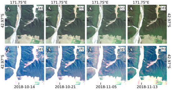
Figure 1.
Sentinel-2 imagery from the Hawdon Valley, South Island, New Zealand, showing a flowering event during the spring of 2018: (a–d) are natural color; (e–h) are natural color with an exaggerated stretch to amplify the “red” band (Band 4). The images are organized by column, e.g., (a,e) are the natural color and stretched color for 14 October 2018, respectively.
In order to detect the yellowing that is associated with southern beech flowering, we applied two approaches: the calculation of a normalized difference yellowing index (NDYI) to describe the red–green band relationship and the modeling of this index over the time series of the image archive to detect variations from the expected (non-flowering) state. The effect is subtle enough that the technique required was very sensitive to cloud and shadow contamination. In addition to the cloud masking performed above, “invalid” pixels from the cloud mask (cloud, shadow, snow or water) were buffered by 30 pixels (300 m) and patches of “valid” pixels smaller than 100 ha were re-classified as “invalid”. Extra spectral filtering was then used to mask the remaining pixels that were too bright or dark to be forest (or useful): . The result was then further buffered by 3 pixels.
The NDYI is similar to the well-known normalized difference vegetation index (NDVI) [32], using the “red” (Band 4665 ± 15 nm) and “green” (Band 3560 ± 18 nm) Sentinel-2 bands instead of the “near-infrared” and “red” bands. It is also very similar to the green-red vegetation index (GRVI) [33,34], with the order of the bands merely reversed:
The NDYI was calculated using the Level-1C TOA reflectance product re-projected to the New Zealand Transverse Mercator (NZTM) coordinate reference system (EPSG:2193) and with any invalid pixels masked. As the NDYI represents the ratio of red–green and both are affected similarly by transient atmospheric conditions, it was negative over most areas of forest most of the time (i.e., when a pixel was “green”), increasing to near or slightly above 0 during heavy flowering events.
Substantial annual variation was present in the TOA reflectance observations over forest due to climatic conditions, vegetation phenology (e.g., new leaves), and sun angle. The NDYI signal visually observed during flowering was subtle enough within the context of a year of data that setting simple thresholds was inadequate to produce a reliable result. Additionally, flowering can occur at different times during the spring season, depending on latitude and altitude [3,8]. The temporal sequence of NDYI for a pixel in the Hawdon Valley (South Island, New Zealand) is shown in Figure 2 as an example. The orange line is a modeled NDYI time series that is unique to that pixel, using an approach similar to that used in the TMASK methodology developed for cloud detection in Landsat 8 imagery [35]. The model used robust regression to calculate unique per pixel () coefficients for the sine and cosine terms for intra- (, ) and inter-annual (, ) variability, as well as a constant term (). Where x is the number of days since the start of the temporal sequence, is the number of days per year, and is the number of days in the sequence:
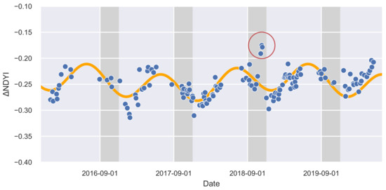
Figure 2.
The observed normalized difference yellowing index (NDYI) time series for an example pixel from Figure 1 in the Hawdon Valley (blue) with superimposed modeled values (orange). The gray areas indicate austral spring seasons (September–November) where the NDYI is expected to peak during a mast. The red circle shows the NDYI that was higher than expected during the spring of 2018 (the “mega-mast” season).
The observed NDYI for each pixel and date were then subtracted from the modeled value for that pixel and date to produce and the maximum value was found for each flowering season (1 September to 10 December) using:
Finally, values were converted into a map of “heavy flowering detected” vs. “heavy flowering not detected” by following a method similar to Shepherd et al. [36]. First, a high threshold of 0.08 was chosen by assessing against seed trap data [4] during the 2018 “mega-mast”. This threshold was used to create “seed” areas, which were grown outward by progressively lowering the threshold to 0.04. The resulting “flowering” pixels were then buffered by 2 pixels, followed by a 5 × 5 majority filter that was then eroded by 2 pixels. “Heavy flowering not detected” patches that were smaller than 1 ha (minimum mapping unit) were removed by being re-coded as “heavy flowering detected” or “no data” (majority of surrounding pixels), then the “heavy flowering detected” patches that were smaller than 1 ha were re-coded as “heavy flowering not detected” to reduce small-scale noise.
As no reliable spatial dataset of beech flowering exists beyond occasional field reports from DOC staff, the national-scale map for the 2018 mast year was accuracy assessed by a human operator. At 1000 randomly selected sites, 500 in “heavy flowering detected” and 500 in “heavy flowering not detected”, the operator determined whether heavy flowering was observed in the temporal sequence of 2018 cloud-free imagery in comparison to a median spring image (excluding 2018). Heavy flowering was easily observed in the temporal progression of spectral reflectance relative to the median image, especially when the spatial extent of the flowering moved upward in elevation as the season progressed (using the exaggerated red band stretch shown in Figure 1). A confusion matrix of proportions was estimated using the method of Card [37], from which precision and recall were calculated [38].
3. Results
The austral spring (September–November) of 2017 was a light flowering season for southern beech in New Zealand. This was followed by a “mega-mast” in 2018, with heavy flowering observed from the ground during spring and a corresponding heavy seed fall the following autumn. Maps of the maximum spring were produced for each year of data, with the results for the 2018 season shown in Figure 3. The spatial patterns corresponded with anecdotal reports from DOC staff who were based at field offices around New Zealand. There was heavy flowering throughout most of the northwestern corner of the South Island and sporadic heavy flowering in eastern Fiordland. The inset of Figure 3 highlights the level of detail available and shows the heavy flowering on the lower slopes of the Hawdon and Poulter Valleys, dissipating as altitude increases up the valley walls (the black areas are not beech forest; they are either alpine or riverbed in this location).
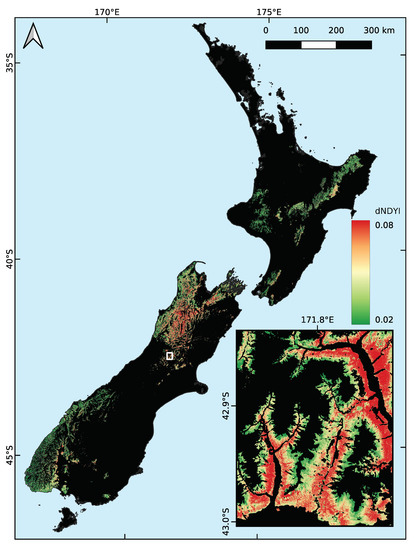
Figure 3.
The maximum (from the model) for spring 2018 in areas of known southern beech forest in New Zealand. Green denotes areas of low (<0.02) maximum , while red is high (>0.08) and indicates heavy beech flowering. The inset shows the Hawdon and Poulter Valleys near Arthur’s Pass (1:250,000 at 42.95°S, 171.82°E; see white box).
Figure 4 shows the maps of heavy beech flowering as detected by our method for years 2017–2021. In spring 2018, a lot of heavy beech flowering was detected in the north-west of the South Island, which was synonymous with a “mega-mast” event in that region. In the North Island and the south-west of the South Island, some pockets of heavy flowering were detected. The following year, in spring 2019, the flowering was much reduced in the north-west of the South Island, but in the North Island, a lot of heavy flowering was detected, which was synonymous with another “mega-mast”. The south-west of the South Island had pockets of heavy flowering, much the same as in 2018. In years 2020 and 2021, minimal beech flowering was detected in most areas.
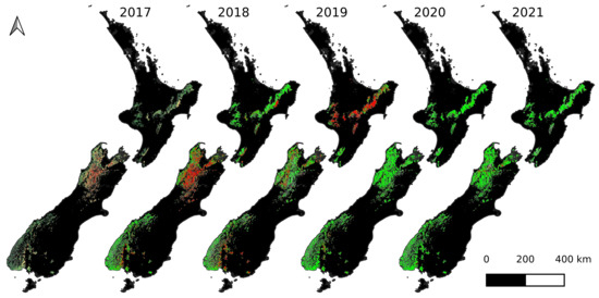
Figure 4.
The maps of heavy beech flowering during spring time for four years using Sentinel-2 imagery (2017–2021 inclusive). The classes are “heavy flowering detected” (red), “heavy flowering not detected” (green), and “no cloud-free imagery” (gray).
In the 2018 map, heavy flowering was detected in 27.6% (1,144,382 ha) of the 4.1 million ha of beech forest in New Zealand. Heavy flowering was not detected in 51.2% (2,122,201 ha) of the beech forest. In the remaining 21.2% of the beech forest (878,406 ha), there was no cloud-free imagery in the spring to enable a decision to be reached. In each of the two classes for “heavy flowering detected” and “heavy flowering not detected”, we generated 500 random locations at which we compared reference data to map data. The reference data were determined from the visual interpretation of all cloud-free spring imagery for that year. Table 1 shows the confusion matrix of proportions. The overall classification accuracy was 90.8%. The precision (user’s accuracy) scores indicate that 90.4% of the area mapped as “heavy flowering detected” was actually heavy flowering. The recall (producer’s accuracy) scores indicate that 84.4% of actual “heavy flowering detected” was successfully mapped as “heavy flowering detected”. The overall F1-score for “heavy flowering detected” was 0.873 and “heavy flowering not detected” was 0.928. Thus, the method is likely to underestimate (slightly), rather than overestimate, areas of heavy flowering; however, the scores reflect well on the method overall.

Table 1.
A confusion matrix showing detected and not detected heavy flowering (proportion of map) for the method (Mapped), assessed against a human operator (Reference). The proportions were estimated from a random sample of 500 locations in the “heavy flowering detected” class (weighted by proportion of “heavy flowering detected” in map = 0.35) and a random sample of 500 locations in the “heavy flowering not detected” class (weighted by 0.65).
4. Discussion
We developed a method that can produce a national map of heavy beech flowering from a temporal sequence of Copernicus Sentinel-2 imagery (Figure 4). The method detects elevated values of a yellow index (NDYI) the are above those normally expected in spring. A value greater than 0.08 indicates especially heavy flowering; however, these regions can be “grown” into adjacent pixels where is greater than 0.04 to better capture all heavy flowering. The elevated yellow index is caused by the production of red flowers that obscure the green leaves. The national map of beech flowering can be produced at the end of spring, several months before the subsequent mast event actually occurs and seeds drop to the ground. It can then be provided to DOC, which is the national agency in charge of pest control, to aid with planning additional pest control to be implemented several months later. In the spring of 2018, a nationwide beech mast event was detected and mapped using this method. A manual accuracy assessment determined the heavy flowering map to have an overall accuracy of 90%. The spatial distribution of beech flowering, as mapped by the method, was also consistent with anecdotal observations from DOC field staff.
The national map of beech flowering can be used to provide extra detail to augment the existing model [7] as it provides a higher spatial resolution of 10 m, as opposed to 5 km. It is also a map of confirmed flowering, which is one less degree of separation from the actual seed fall than the model, as physical factors, such as carbon availability and soil moisture conditions, also affect flowering and seed productivity [39]. However, one issue with our method is the requirement for cloud-free satellite imagery at critical flowering times. This means that flowering may have been missed in some areas, which effectively makes the map a better indicator of “presence” rather than “absence”.
Not all heavy beech flowering in spring results in heavy seed fall in the following autumn. Heavy frost or very wet weather can interfere with seed production [3]. Figure 5 shows how well the maximum compared to seed counts in trays located on the floor of the beech forest (seed traps are spread throughout beech forests in New Zealand as part of a long-running monitoring program conducted by DOC [4]). Data were restricted to locations with at least eight valid observations in order to obtain representation over the majority of the spring season. There was noise in the data, nevertheless high seed counts generally corresponded with high maximum ( = 0.397). For reference, the model had values between 0.331 and 0.556 for the same species range [7] (although that study used the older genus name Nothofagus). Reasons for the mismatches between the and seed count include: cloud coverage still obscuring the flowering event, despite the high number of revisits (low vs. high seed count); inaccurate trap location (variable impact on relationship); trap location relative to flowering trees combined with wind direction during seed fall (high vs. low seed count); different beech species (different relationship between and seed count); climate, adverse weather events, and nutrient availability (lower seed count vs. higher ); and inaccuracies in the method (addressed in accuracy assessment). We recommend that the national map of flowering/not flowering be regarded as a map of potential high seed fall for initial planning purposes, which is to be confirmed later with additional information, such as selected field observations.
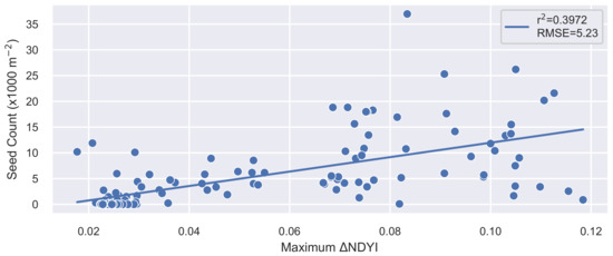
Figure 5.
The relationship between the maximum (spring 2018) and the number of seeds collected from seed traps in the permanent trap network (autumn/winter 2019) for the 2018/2019 masting season. The locations are filtered to exclude those with fewer than eight valid satellite observations.
One way to address the paucity of valid observations would be to add more data sources. As the technique developed in this study relies only on red, green, blue, and NIR (for quality control) wavelengths, it should be possible to include data from commercial satellite constellations that have higher revisit rates but lower spectral ranges or resolutions, such as the Planet “Dove” constellation. Adding freely available Landsat 8 data could also increase the probability of obtaining valid observations at critical times. Targeted aerial imaging campaigns could also provide valuable information in areas of known data paucity, particularly when they are informed by observations from field staff. This study has shown that the resolution requirement is low, by aerial imaging standards, which would allow for higher flight altitudes and larger image footprints, thereby substantially reducing cost. Multiple studies have shown that the fusion of these separate data sources is useful in remote sensing [11,14,16,20,40,41], though the spatial complexity and rugged terrain of the beech forests in New Zealand is likely to reduce the utility of the coarse resolution MODIS optical imagery.
This study successfully mapped the presence of heavy flowering in beech trees at a large scale (greater than 4 million ha) using a visible change in canopy color. A similar study by Garcia et al. [21] was less successful, but did show that moisture-based indices in the lead-up to a flowering or seed/cone event could provide additional information. Fernández-Martínez et al. [19] were also successful in predicting mast events using a combination of the enhanced vegetation index (EVI) and weather data during spring. A number of challenges exist in the context of detecting mast events and the approach attempts to minimize these. The NDYI index was chosen to specifically target the red and green image bands, avoiding the red edge and near-infrared bands that also respond to vegetation conditions and thus, increase noise. The effectiveness of the multi-year sine and cosine model for modeling the typical behaviour of NDYI, the utilization of extreme values as “seeds” for regions that grow into areas of lower values, and the ability to tune the spectral value constraints all contribute to the effectiveness of our approach. To further improve the performance of the method, it would be worth investigating the use of supporting indices, such as Garcia et al. [21] and Fernández-Martínez et al. [19], in addition to adding extra data sources. Further work into distinguishing different beech species would also add greater value for DOC as those with larger seeds (red and hard beech) have a disproportionately larger impact on rodent irruption.
The temporal analysis of Sentinel-2 satellite imagery has proven to be successful at detecting heavy flowering in New Zealand beech forests. To achieve this, cloud clearing had to be accurate (because the yellow index is sensitive to missed cloud) and automated (because many images are required). The automation of the cloud clearing [31] and other processing means that beech flowering maps can be produced in a timely and cost-effective way. In future, we plan to produce a national map of heavy beech flowering at the end of each spring. This would allow for several months of analysis to plan the extra pest control that would be required in the autumn, thereby improving targeted pest control in masting areas and leading to better outcomes for native fauna.
5. Conclusions
This study used Sentinel-2 top of atmosphere (TOA) imagery to detect and map atypical yellowing that was associated with the heavy flowering of southern beech (Fuscospora and Lophozonia) forests in New Zealand over 4.1 million ha at an unprecedented 10 m spatial resolution. This was achieved by modeling a normalized difference yellowing index (NDYI) over 5 years of observation and investigating any deviations from the expected values during spring months (September–November). A “threshold” value of 0.08 was used to identify areas of heavy flowering, with connected areas of > 0.04 also likely flowering. The method was automated and could be run for all of New Zealand in less than a day on a cluster of approximately 1000 CPU cores. Using Sentinel-2 imagery, the method typically provided information on heavy flowering for 80% of the beech forests in New Zealand with a high overall classification accuracy of 90.8%, resulting in useful information for the planning of national-scale pest control efforts.
Author Contributions
Conceptualization, B.J., J.R.D., T.G. and J.S.; data curation, B.J., J.D.S. and J.S.; formal analysis, B.J.; funding acquisition, J.R.D.; investigation, B.J., J.R.D. and T.G.; methodology, B.J., J.R.D., J.D.S. and T.G.; project administration, J.R.D.; resources, J.R.D.; software, B.J., J.D.S. and J.S.; supervision, J.R.D.; visualization, B.J.; writing—original draft, B.J.; writing—review and editing, J.R.D., J.S. and T.G. All authors have read and agreed to the published version of the manuscript.
Funding
This research was funded by the New Zealand Ministry of Business, Innovation and Employment (MBIE) Endeavour Fund, under the Advanced Remote Sensing of Aotearoa research program (C09X1709).
Data Availability Statement
Data available on reasonable request.
Acknowledgments
The authors would like to thank the New Zealand Department of Conservation (DOC) for providing advice and validation data.
Conflicts of Interest
The authors declare no conflict of interest. The funders had no role in the design of the study, in the collection, analyses or interpretation of data, in the writing of the manuscript or in the decision to publish the results.
Abbreviations
The following abbreviations are used in this manuscript:
| DOC | Department of Conservation |
| EBI | Enhanced Bloom Index |
| ESA | European Space Agency |
| EVI | Enhanced Vegetation Index |
| GRVI | Green-Red Vegetation Index |
| NDVI | Normalized Difference Vegetation Index |
| NDYI | Normalized Difference Yellowing Index |
| NZTM | New Zealand Transverse Mercator |
| TOA | Top of Atmosphere |
References
- Heenan, P.B.; Smissen, R.D. Revised circumscription of Nothofagus and recognition of the segregate genera Fuscospora, Lophozonia, and Trisyngyne (Nothofagaceae). Phytotaxa 2013, 146, 1–31. [Google Scholar] [CrossRef]
- Shepherd, J.R.D.; Ausseil, A.G.; Dymond, J.R. EcoSat Forests: A 1: 750,000 Scale Map of Indigenous Forest Classes in New Zealand; Manaaki Whenua Press: Lincoln, New Zealand, 2005. [Google Scholar]
- Wardle, J.A. The New Zealand Beeches. Ecology, Utilisation and Management; New Zealand Forest Service: Wellington, New Zelaand, 1984; p. 477.
- Elliott, G.; Kemp, J. Large-scale pest control in New Zealand beech forests. Ecol. Manag. Restor. 2016, 17, 200–209. [Google Scholar] [CrossRef]
- Ruscoe, W.A.; Pech, R.P. Rodent Outbreaks: Ecology and Impacts. In Rodent Outbreaks: Ecology and Impacts; Singleton, G., Belmain, S., Brown, P., Hardy, B., Eds.; Internationl Rice Research Institute: Los Baños, Philippines, 2010; pp. 239–251. [Google Scholar]
- King, C.M.; Powell, R.A. Managing an invasive predator pre-adapted to a pulsed resource: A model of stoat (Mustela erminea) irruptions in New Zealand beech forests. Biol. Invasions 2011, 13, 3039–3055. [Google Scholar] [CrossRef]
- Kelly, D.; Geldenhuis, A.; James, A.; Penelope Holland, E.; Plank, M.J.; Brockie, R.E.; Cowan, P.E.; Harper, G.A.; Lee, W.G.; Maitland, M.J.; et al. Of mast and mean: Differential-temperature cue makes mast seeding insensitive to climate change. Ecol. Lett. 2013, 16, 90–98. [Google Scholar] [CrossRef] [PubMed]
- Allen, R.B.; Hurst, J.M.; Portier, J.; Richardson, S.J. Elevation-dependent responses of tree mast seeding to climate change over 45 years. Ecol. Evol. 2014, 4, 3525–3537. [Google Scholar] [CrossRef] [PubMed]
- Bogdziewicz, M.; Kelly, D.; Thomas, P.A.; Lageard, J.G.; Hacket-Pain, A. Climate warming disrupts mast seeding and its fitness benefits in European beech. Nat. Plants 2020, 6, 88–94. [Google Scholar] [CrossRef]
- Bogdziewicz, M.; Hacket-Pain, A.; Kelly, D.; Thomas, P.A.; Lageard, J.; Tanentzap, A.J. Climate warming causes mast seeding to break down by reducing sensitivity to weather cues. Glob. Chang. Biol. 2021, 27, 1952–1961. [Google Scholar] [CrossRef]
- Bolton, D.K.; Gray, J.M.; Melaas, E.K.; Moon, M.; Eklundh, L.; Friedl, M.A. Continental-scale land surface phenology from harmonized Landsat 8 and Sentinel-2 imagery. Remote Sens. Environ. 2020, 240, 111685. [Google Scholar] [CrossRef]
- Misra, G.; Cawkwell, F.; Wingler, A. Status of phenological research using sentinel-2 data: A review. Remote Sens. 2020, 12, 2760. [Google Scholar] [CrossRef]
- Zeng, L.; Wardlow, B.D.; Xiang, D.; Hu, S.; Li, D. Remote Sensing of Environment A review of vegetation phenological metrics extraction using time-series, multispectral satellite data. Remote Sens. Environ. 2020, 237, 111511. [Google Scholar] [CrossRef]
- Dixon, D.J.; Callow, J.N.; Duncan, J.M.; Setterfield, S.A.; Pauli, N. Satellite prediction of forest flowering phenology. Remote Sens. Environ. 2021, 255, 112197. [Google Scholar] [CrossRef]
- Moon, M.; Seyednasrollah, B.; Richardson, A.D.; Friedl, M.A. Using time series of MODIS land surface phenology to model temperature and photoperiod controls on spring greenup in North American deciduous forests. Remote Sens. Environ. 2021, 260, 112466. [Google Scholar] [CrossRef]
- Moon, M.; Richardson, A.D.; Friedl, M.A. Multiscale assessment of land surface phenology from harmonized Landsat 8 and Sentinel-2, PlanetScope, and PhenoCam imagery. Remote Sens. Environ. 2021, 266, 112716. [Google Scholar] [CrossRef]
- Browning, D.M.; Russell, E.S.; Ponce-Campos, G.E.; Kaplan, N.; Richardson, A.D.; Seyednasrollah, B.; Spiegal, S.; Saliendra, N.; Alfieri, J.G.; Baker, J.; et al. Monitoring agroecosystem productivity and phenology at a national scale: A metric assessment framework. Ecol. Indic. 2021, 131, 108147. [Google Scholar] [CrossRef]
- Atkinson, P.M.; Jeganathan, C.; Dash, J.; Atzberger, C. Inter-comparison of four models for smoothing satellite sensor time-series data to estimate vegetation phenology. Remote Sens. Environ. 2012, 123, 400–417. [Google Scholar] [CrossRef]
- Fernández-Martínez, M.; Garbulsky, M.; Peñuelas, J.; Peguero, G.; Espelta, J.M. Temporal trends in the enhanced vegetation index and spring weather predict seed production in Mediterranean oaks. Plant Ecol. 2015, 216, 1061–1072. [Google Scholar] [CrossRef]
- Cheng, Y.; Vrieling, A.; Fava, F.; Meroni, M.; Marshall, M.; Gachoki, S. Phenology of short vegetation cycles in a Kenyan rangeland from PlanetScope and Sentinel-2. Remote Sens. Environ. 2020, 248, 112004. [Google Scholar] [CrossRef]
- Garcia, M.; Zuckerberg, B.; Lamontagne, J.M.; Townsend, P.A. Landsat-based detection of mast events in white spruce (Picea glauca) forests. Remote Sens. Environ. 2021, 254, 112278. [Google Scholar] [CrossRef]
- Noumonvi, K.D.; Oblišar, G.; Žust, A.; Vilhar, U. Empirical approach for modelling tree phenology in mixed forests using remote sensing. Remote Sens. 2021, 13, 3015. [Google Scholar] [CrossRef]
- Asokan, A.; Anitha, J. Change detection techniques for remote sensing applications: A survey. Earth Sci. Inform. 2019, 12, 143–160. [Google Scholar] [CrossRef]
- Panuju, D.R.; Paull, D.J.; Griffin, A.L. Change detection techniques based on multispectral images for investigating land cover dynamics. Remote Sens. 2020, 12, 1781. [Google Scholar] [CrossRef]
- Chen, B.; Jin, Y.; Brown, P. An enhanced bloom index for quantifying floral phenology using multi-scale remote sensing observations. ISPRS J. Photogramm. Remote Sens. 2019, 156, 108–120. [Google Scholar] [CrossRef]
- Dymond, J.R.; Shepherd, J.R.D. The spatial distribution of indigenous forest and its composition in the Wellington region, New Zealand, from ETM+ satellite imagery. Remote Sens. Environ. 2004, 90, 116–125. [Google Scholar] [CrossRef]
- Landcare Research Ltd. EcoSat Forests (North Island); Landcare Research Ltd.: Lincoln, New Zealand, 2014. [Google Scholar] [CrossRef]
- Landcare Research Ltd. EcoSat Forest (South Island); Landcare Research Ltd.: Lincoln, New Zealand, 2014. [Google Scholar] [CrossRef]
- Department of Conservation. Flowering and Fruit Production; Department of Conservation: Wellington, New Zealand, 2019.
- Department of Conservation. Department of Conservation Te Papa Atawhai Annual Report 2019; Technical Report; Department of Conservation: Wellington, New Zealand, 2019.
- Shepherd, J.R.D.; Schindler, J.; Dymond, J.R. Automated Mosaicking of Sentinel-2 Satellite Imagery. Remote Sens. 2020, 12, 3680. [Google Scholar] [CrossRef]
- Rouse, W.; Haas, H.; Deering, W. Monitoring vegetation systems in the Great Plains with ERTS. In Goddard Space Flight Center 3d ERTS-1 Symposium; NASA: Greenbelt, MD, USA, 1974. [Google Scholar]
- Tucker, C.J. Red and Photographic Infrared l, lnear Combinations for Monitoring Vegetation. Remote Sens. Environ. 1979, 8, 127–150. [Google Scholar] [CrossRef] [Green Version]
- Motohka, T.; Nasahara, K.N.; Oguma, H.; Tsuchida, S. Applicability of Green-Red Vegetation Index for remote sensing of vegetation phenology. Remote Sens. 2010, 2, 2369–2387. [Google Scholar] [CrossRef] [Green Version]
- Zhu, Z.; Woodcock, C.E. Automated cloud, cloud shadow, and snow detection in multitemporal Landsat data: An algorithm designed specifically for monitoring land cover change. Remote Sens. Environ. 2014, 152, 217–234. [Google Scholar] [CrossRef]
- Shepherd, J.R.D.; Dymond, J.R.; Cuff, J.R. Monitoring scrub weed change in the Canterbury region using satellite imagery. N. Z. Plant Prot. 2007, 60, 137–140. [Google Scholar] [CrossRef]
- Card, D.H. Using Known Map Category Marginal Frequencies to Improve Estimates of Thematic Map Accuracy. Photgrammetric Eng. Remote Sens. 1982, 48, 431–439. [Google Scholar]
- Maxwell, A.E.; Warner, T.A.; Guillén, L.A. Accuracy assessment in convolutional neural network-based deep learning remote sensing studies—Part 1: Literature review. Remote Sens. 2021, 13, 2450. [Google Scholar] [CrossRef]
- Uscoe, W.E.A.R.; Latt, K.E.H.P.; Richardson, S.J.; Allen, R.B.; Whitehead, D.; Carswell, F.E.; Ruscoe, W.A.; Platt, K.H. Climate and net carbon availability determine temporal patterns of seed production by Nothofagus. Ecology 2005, 86, 972–981. [Google Scholar]
- Thapa, S.; Millan, V.E.G.; Eklundh, L. Assessing forest phenology: A multi-scale comparison of near-surface (UAV, spectral reflectance sensor, phenocam) and satellite (MODIS, sentinel-2) remote sensing. Remote Sens. 2021, 13, 1597. [Google Scholar] [CrossRef]
- Peng, D.; Wang, Y.; Xian, G.; Huete, A.R.; Huang, W.; Shen, M.; Wang, F.; Yu, L.; Liu, L.; Xie, Q.; et al. Investigation of land surface phenology detections in shrublands using multiple scale satellite data. Remote Sens. Environ. 2021, 252, 112133. [Google Scholar] [CrossRef]
Publisher’s Note: MDPI stays neutral with regard to jurisdictional claims in published maps and institutional affiliations. |
© 2022 by the authors. Licensee MDPI, Basel, Switzerland. This article is an open access article distributed under the terms and conditions of the Creative Commons Attribution (CC BY) license (https://creativecommons.org/licenses/by/4.0/).