Estimating High-Resolution PM_2.5 Concentrations by Fusing Satellite AOD and Smartphone Photographs Using a Convolutional Neural Network and Ensemble Learning

Abstract

Aerosol optical depth (AOD) data derived from satellite products have been widely used to estimate fine particulate matter (PM_2.5) concentrations. However, existing approaches to estimate PM_2.5 concentrations are invariably limited by the availability of AOD data, which can be missing over large areas due to satellite measurements being obstructed by, for example, clouds, snow cover or high concentrations of air pollution. In this study, we addressed this shortcoming by developing a novel method for determining PM_2.5 concentrations with high spatial coverage by integrating AOD-based estimations and smartphone photograph-based estimations. We first developed a multiple-input fuzzy neural network (MIFNN) model to measure PM_2.5 concentrations from smartphone photographs. We then designed an ensemble learning model (AutoELM) to determine PM_2.5 concentrations based on the Collection-6 Multi-Angle Implementation of Atmospheric Correction AOD product. The R² values of the MIFNN model and AutoELM model are 0.85 and 0.80, respectively, which are superior to those of other state-of-the-art models. Subsequently, we used crowdsourced smartphone photographs obtained from social media to validate the transferability of the MIFNN model, which we then applied to generate smartphone photograph-based estimates of PM_2.5 concentrations. These estimates were fused with AOD-based estimates to generate a new PM_2.5 distribution product with broader coverage than existing products, equating to an average increase of 12% in map coverage of PM_2.5 concentrations, which grows to an impressive 25% increase in map coverage in densely populated areas. Our findings indicate that the robust estimation accuracy of the ensemble learning model is due to its detection of nonlinear correlations and high-order interactions. Furthermore, our findings demonstrate that the synergy of smartphone photograph-based estimations and AOD-based estimations generates significantly greater spatial coverage of PM_2.5 distribution than AOD-based estimations alone, especially in densely populated areas where more smartphone photographs are available.

1. Introduction

Over the past few decades, urban environmental pollution, especially air pollution, has become a major problem in many countries around the world [1,2]. Pollution comprising fine particulate matter (PM${}_{2.5}$), consisting of solid or liquid particles suspended in the air that have aerodynamic diameters of 2.5 micrometers or less, has a substantially greater adverse effect on human health than other types of pollution, as it remains suspended in the atmosphere for a long time and can pass through the throat or nasal cavity to penetrate deep into the lungs, bloodstream, or brain [3,4], which can elevate the incidence of many a disease, including lung cancer [5], cerebrovascular diseases [6], cardiovascular diseases [7] and respiratory-related diseases [8]. The China National Environmental Monitoring Centre (CNEMC) launched a national network to monitor air pollution, including PM${}_{2.5}$, in 2012, but its ground-based monitoring stations are generally located in densely populated megacities and have an effective monitoring range of only 3 km [9]. Thus, in areas that far from ground-based monitors, accurate air-quality information cannot be obtained from these stations and nor can their data be used to conduct exposure assessments.

The rapid growth of satellite remote-sensing technologies in the past 20 years has led to the discovery of the strong correlation between PM${}_{2.5}$ concentrations and aerosol optical depth (AOD), a satellite product defined as the integration of aerosol extinction, which can represent optical properties. Consequently, various satellite-derived AOD products have been widely applied, such as those generated by the Moderate Resolution Imaging Spectroradiometer (MODIS) [10,11,12,13,14,15], the Multi-angle Imaging Spectro-Radiometer (MISR) [10,16], the Visible Infrared Imaging Radiometer Suite (VIIRS) [17,18], and the Multi-Angle Implementation of Atmospheric Correction (MAIAC) [19,20]. In these studies, the AOD products have typically been integrated with ancillary variables, such as meteorological data and geographical data, to improve model performance [14,15]. MODIS AOD data are the most commonly used, and the strong correlation of these data with PM${}_{2.5}$ concentrations has been proven in many studies [13,14,15].

Given the association between AOD data and ground-level PM${}_{2.5}$ concentrations, a variety of models have been developed, including the chemical transport model [16], a semi-empirical model [12], the linear mixed effect model [11], the land-use regression model [21], the geographically weighted regression (GWR) model [22], and the geographically and temporally weighted regression (GTWR) model [13,14]. These models can generate results with $R^2$ values ranging from 0.54 to 0.80. More recently, researchers have begun to develop machine learning models, owing to their superiority to other models for solving complicated nonlinear problems. In addition, an ensemble model can outperform any of its base models, and reduce the spread or dispersion of estimates by integrating the features of base models. For instance, a space-time random forest model based on an ensemble regression model and the interaction of spatiotemporal information was developed to estimate daily PM${}_{2.5}$ concentrations across China, with an overall $R^2$ of 0.85 [15]. In another example, an interpretable convolutional neural network (CNN) was designed and trained using MODIS AOD products to estimate PM${}_{2.5}$ concentrations over the United States, with a temporally-separated CV $R^2$ of 0.83 and a spatially-separated CV $R^2$ of 0.69, respectively [23]. Similarly, given the advantages of ensemble models, a stacking model was developed by integrating boost networks and neural networks (NNs), which outperformed its three base models by an average of 8% [24].

However, these methods are invariably restricted by the availability of AOD data, which are often unavailable for large areas due to misclassifications caused by external factors such as clouds, snow cover, or severe air pollution. This problem cannot be effectively solved by fusing multiple sets of AOD data, as they may all be affected by these external factors. One promising approach to solve this problem is complementing AOD data with air quality data derived from smartphone photographs, as the growing popularity and development of smartphone cameras makes obtaining high-quality smartphone photographs simple and convenient. Several image analysis-based methods for the estimation of PM${}_{2.5}$ concentrations from photographs have been developed in the past few years, including image feature-based methods and NN-based methods. Image feature-based methods scrutinize the relationship between image features and airborne PM${}_{2.5}$. First, PM${}_{2.5}$-related features are extracted by analyzing image characteristics, such as transmission [25,26,27], image entropy [25], image contrast [25,26]; and sky color [25], and then the relationship between extracted features and PM${}_{2.5}$ concentrations is determined by the use of a model, such as a linear regression model [26], a support-vector regression [25], a generic model [27], or an NN [28]. NN-based methods exploit the flexibility of NNs for solving computer vision problems, and have been successfully applied to extreme weather forecasting [29], traffic sign detection [30], and atmospheric particle identification or classification [31]. First, studies focused on classifying photographs into several groups in terms of air pollution concentrations [32]. Later, Bo et al. [33] used a CNN to estimate PM${}_{2.5}$ indices from photographs by combining photographic information with two weather features: humidity and wind speed. Subsequently, many CNN-based methods and optimizations were developed to estimate PM${}_{2.5}$ concentrations from photographs, such as by utilizing high-level features extracted by CNN models [34], ensemble learning [35], a gradient boosting machine [36], feature fuzzification [37], and information abundance measurements [28]. However, the high sensitivity of some photographic features to various factors means that they cannot be used as haze-relevant features; for example, sky color is strongly affected by weather. In addition, many methods can only estimate the PM${}_{2.5}$ concentrations at a fixed location, as their robustness has not been validated on datasets from other locations.

We solved the above problems by developing a method for determining PM${}_{2.5}$ concentrations with wider spatial coverage by integrating AOD-based estimations with smartphone photograph-based estimations. First, we developed a fuzzy neural network with multiple inputs (smartphone photographs and image features), denoted MIFNN, to estimate the PM${}_{2.5}$ concentration from a single smartphone photograph taken in any location, rather than only in a single location. Next, we constructed an ensemble learning model, AutoELM, from multiple base models: the random forest model, the CatBoost model [38], the extreme gradient boosting (XGBoost) model [39], the light gradient boosting machine (LightGBM) [40], and some NNs. AutoELM was then applied to generate the daily PM${}_{2.5}$ distribution in Beijing from MODIS 1 km MAIAC AOD data (the primary predictor) combined with meteorological and geographical field data. Subsequently, fusion of the results from the MIFNN model and the AutoELM afforded a new PM${}_{2.5}$ distribution product with higher spatial coverage than its precursors. Several commonly used metrics were applied to evaluate the performance of the model or to quantify the correlation between estimated values and actual values, including the root-mean-square error (RMSE), the Pearson correlation coefficient (r), and the coefficient of determination (R-squared) (R${}^2$).

2. Study Area and Data

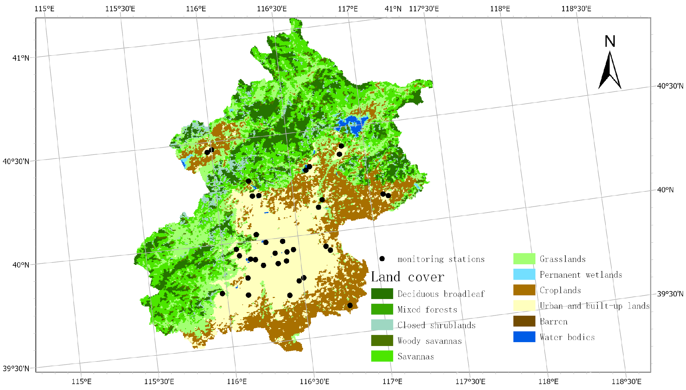
2.1. Study Area

We used Beijing (39–41°N, 115–118°E) as the study area. A recent report from the Center for Strategic and International Studies [41] states that the average PM${}_{2.5}$ concentration in Beijing in 2020 was slightly less than 38.7 µg/m${}^3$ and the Air Quality Index (AQI) was nearly 109, making the PM${}_{2.5}$ concentration seven times higher than the air quality guideline recommended by the World Health Organization (WHO). Figure 1 depicts the spatial distribution of the 35 ground-level monitoring stations in Beijing, which provide hourly measurements of PM${}_{2.5}$ concentrations.

2.2. Data and Processing

The datasets that we used in this study contain photographs with corresponding PM${}_{2.5}$ concentrations or geographical locations, hourly ground-level PM${}_{2.5}$ concentrations, satellite AOD products, and ancillary data that affect the distribution of PM${}_{2.5}$, including meteorological and geographical variables.

2.2.1. Smartphone Photographic Data

We obtained smartphone photographic data from public datasets, by manual collection, and from social media. The two public datasets were shared by [33]: a Shanghai dataset of photographs taken at a fixed location (Oriental Pearl Tower), every 15 min between 10:00 a.m. and 3:00 p.m. of days from May to December of 2014; and a Beijing dataset of photographs of various scenes (including buildings, lakes, roads, and mountains), taken at random hours of days from January to December of 2016. We discarded all smartphone photographs taken at nighttime or that were distorted (such as by rain or snow), which yielded a dataset of 2646 smartphone photographs. We captured an additional 1376 photographs with our smartphones during daytime (ranging from 10:00 a.m. to 4:30 p.m.) in different places from January to December of 2020, where we also measure the PM${}_{2.5}$ concentrations with portable air quality sensors (Nature Clean AM-300; http://www.aiqiworld.com/topic_1049.html, accessed on 14 February 2022). We downloaded smartphone photographs posted on social media from three crowdsourcing websites, including the Institute of Public and Environmental Affairs (a non-profit organization that develops pollution databases), Moji Weather (a social application that generates real-time weather data), and Weibo (a Chinese microblogging website), and we discarded those without geographical location data to obtain a social media photograph dataset of geographically identifiable smartphone photographs.

We collectively denote the above datasets (the refined public dataset and the dataset collected by us) the public photographs and collected photographs (PPCP) dataset, and we used this dataset to train and validate the MIFNN model. We used the social media photographs (SMP) dataset to validate the transferability of the MIFNN model and, in combination with AOD-based estimations, to generate a more accurate and geographically broader estimate of PM${}_{2.5}$ concentrations than that obtainable from AOD-based estimations alone (see Section 3 for more details).

2.2.2. Ground-Based PM_2.5 Concentration Data

Ground-based PM${}_{2.5}$ concentration data from 1 January 2021 to 31 December 2021 were acquired from Beijing Municipal Ecological and Environmental Monitoring Center (http://www.bjmemc.com.cn/, accessed on 14 February 2022), which publishes hourly air-pollutant concentrations from the 35 ground-based monitoring stations presented in Figure 1.

2.2.3. Satellite AOD

We employed MODIS daily 1 km MAIAC AOD products at Level 2 (MCD19A2 V6 data), which retrieve AOD data by combining data from the Terra and Aqua satellites [42]. The 550-µm (Optical_Depth_055) AOD products from 1 January 2021 to 31 December 2021 were downloaded from NASA (https://search.earthdata.nasa.gov/, accessed on 14 February 2022).

2.2.4. Ancillary Data

Meteorological variables: We used data of five meteorological variables: wind speed (WS), temperature (TEMP), pressure (PS), boundary layer height (BLH), and relative humidity (RH). The WS, TEMP, PS, and BLH data were downloaded from the European Centre for Medium-Range Weather Forecasts ERA5 dataset (https://www.ecmwf.int/en/forecasts/datasets/reanalysis-datasets/era5, accessed on 14 February 2022), which offers hourly estimates of a vast number of atmospheric, oceanic, and terrestrial variables, and the relative humidity data were calculated from dewpoint temperatures and temperatures in the ERA5 dataset.

Geographical variables: We used elevation and the normalized difference vegetation index (NDVI) as geographical variables. Elevation was represented by a digital elevation model (DEM) obtained from Shuttle Radar Topography Mission data, which has a resolution of 30 m (https://www.usgs.gov/, accessed on 14 February 2022). The NDVI dataset was acquired from the MOD13A2 Version 6 product (https://lpdaac.usgs.gov/products/mod13a2v006/, accessed on 14 February 2022), which provides vegetation index values with a 1 km spatial resolution every 16 days.

2.2.5. Data Processing

We manually excluded smartphone photographs of indoor scenes from the SMP dataset (as the MIFNN model is designed only for photographs of outside scenes), and photographs taken on rainy or snowy days. The remaining smartphone photographs in the SMP dataset were used to improve the coverage of the estimates of PM${}_{2.5}$ distribution generated from satellite AOD data.

Table 1. List of data used in this study.

Variable	Unit	Spatial Scale	Temporal Resolution
PPCP	Count	Lat × Lng	N/A
SMP	Count	Lat × Lng	N/A
AOD	N/A	1 km	Daily
WS	m· s${}^{-1}$	$0.1^{\circ }\times 0.1^{\circ }$	Hourly
TEMP	C	$0.1^{\circ }\times 0.1^{\circ }$	Hourly
PS	Pa	$0.1^{\circ }\times 0.1^{\circ }$	Hourly
RH	%	$0.1^{\circ }\times 0.1^{\circ }$	Hourly
BLH	m	$0.{25}^{\circ }\times 0.{25}^{\circ }$	Hourly
DEM	m	30 m	N/A
NDVI	N/A	1 km	16-day

lists all of the independent variables used in the model development. As the objective of this study was to determine the distribution of PM${}_{2.5}$ at a 1 km spatial resolution, the datasets were first resampled to a 1 km spatial resolution (181 rows × 233 columns) using bilinear interpolation. Given that MODIS only provides AOD data collected at approximately 10:30 a.m. and 1:30 p.m. local time, the hourly ERA5 meteorological data and in situ PM${}_{2.5}$ concentrations covering these times were averaged, and these averages were used as the daily values. Finally, we incorporated these processed independent variables with ground-level PM${}_{2.5}$ concentrations to give 4874 matched samples covering a period of 202 days.

3. Methodology

In this study, we developed a method for combining smartphone photographic data with satellite AOD data to generate estimates of PM${}_{2.5}$ concentrations across a broader geographic range than can be generated from satellite AOD data alone. Hence, we first developed a CNN model (the MIFNN model) that we used to estimate the PM${}_{2.5}$ concentration from a single smartphone photograph, and then used an ensemble learning model (the AutoELM model) to generate a distribution of PM${}_{2.5}$ concentrations from satellite AOD products combined with meteorological and geographical data. Subsequently, we validated the transferability of the MIFNN model and then generated estimated PM${}_{2.5}$ concentrations by fusing the smartphone photograph-based estimations with AOD-based estimations. Crucially, these estimated PM${}_{2.5}$ concentrations span a broader geographical area than can be obtained by using AOD-based estimations alone. A brief flowchart of our method is given in Figure 2.

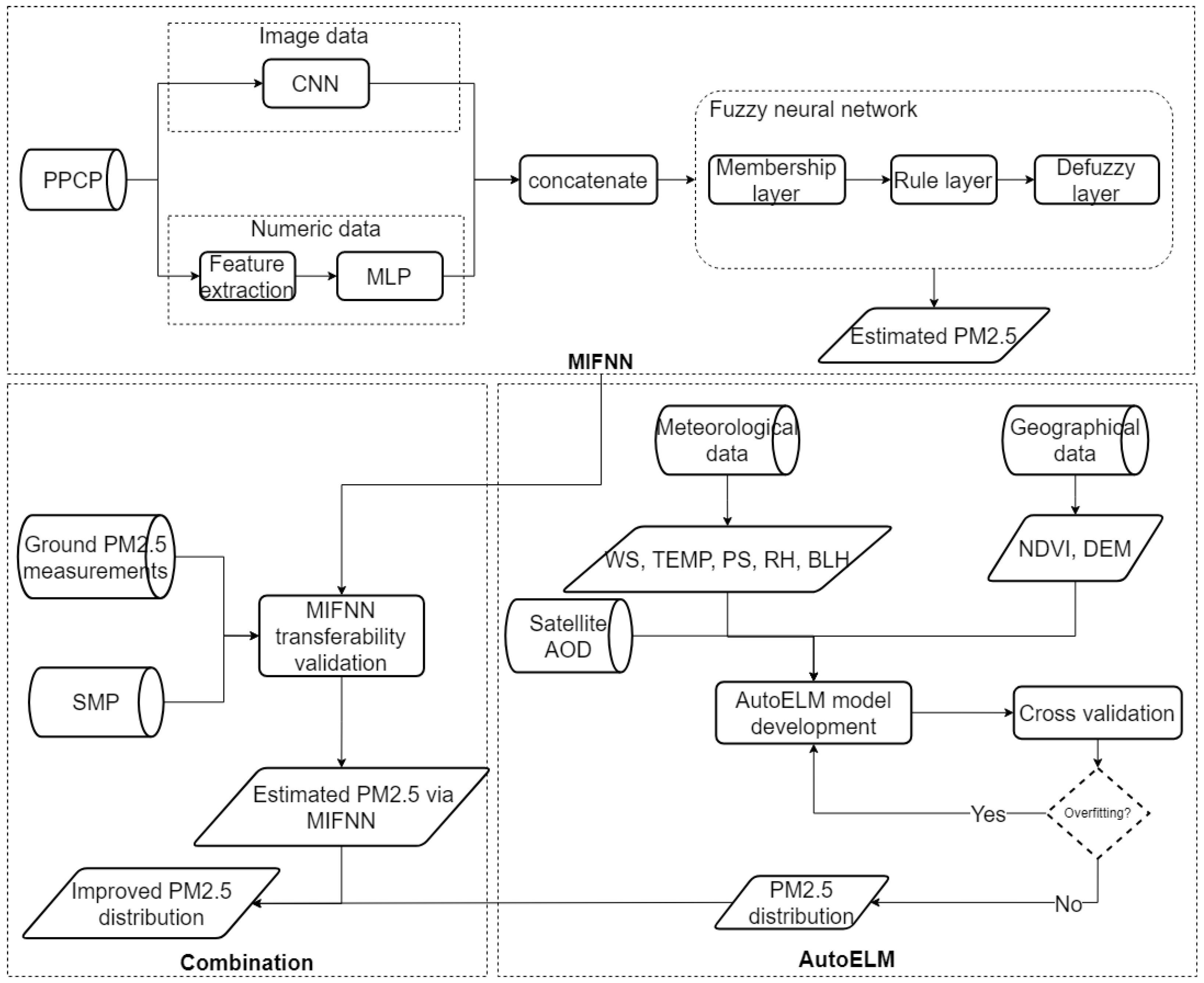
3.1. Smartphone Photograph-Based Estimation of PM_2.5 Concentrations via an NN

We developed the MIFNN model to learn haze-relevant features from smartphone photographs, such that it can estimate PM${}_{2.5}$ concentrations from a single smartphone photograph. The MIFNN model uses two feature-extraction methods to achieve this: physics-based feature extraction and CNN-based feature extraction. In addition, it uses fuzzy logic to increase the reliability of sample data. The structure of the MIFNN model is shown in the upper part of Figure 2.

3.1.1. Physics-Based Feature Extraction

Based on the findings of previous studies [25,26,27,43], we selected the three most important image features that affect PM${}_{2.5}$ concentrations: transmission, image entropy, and image contrast.

A.

Transmission

Image-based methods examine the relationship between relevant image features and PM in the air. PM scatters light in various ways, such as by Mie scattering and Rayleigh scattering, which have a variety of effects on an optical image [44]. In particular, light scattering in hazy environments can degrade visibility, which results in images captured in such environments being blurry. The formation of a hazy image can be described with a haze model and also by an optical model, as shown below [45,46]:

$$I\left(x\right)=J\left(x\right)t\left(x\right)+A(1-t(x\left)\right)$$

(1)

where $I\left(x\right)$ is the observed image, $J\left(x\right)$ is scene radiance, and A is the global atmospheric light. The first term of Equation (1) describes the scene radiance and its degradation in the atmosphere, and the second term represents airlight, which is the light scattered by atmospheric molecules and PM [47]. $t\left(x\right)$ is transmission, an important meteorological parameter that indicates the portion of light that passes through the atmosphere without being scattered, and is expressed by the Beer–Lambert law, as follows [48]:

$$t\left(x\right)=exp(-\beta d(x\left)\right)$$

(2)

where $\beta$ is the atmospheric attenuation coefficient and $d\left(x\right)$ is the scene depth, which describes the distance between the scene and the camera. As PM${}_{2.5}$ is considered to be a primary contributor to light extinction [49], $t\left(x\right)$ and $d\left(x\right)$ are two important image features that can be used for estimating air quality. Moreover, Liu et al. [26] determined that there is an exponential relationship between $t\left(x\right)$ map and PM${}_{2.5}$ concentrations.

In 2010, He et al. [50] proposed dark channel prior theory, which is based on a haze model and the assumption that in most of a haze-free image’s non-sky blocks, at least one color channel has some pixels with very low intensities. The dark channel of an image J can thus be expressed as:

$$J^{dark}\left(x\right)=\underset{c\in \{r,g,b\}}{min}(\underset{y\in \mathsf{\Omega }\left(x\right)}{min}\left(J^c\left(y\right)\right))$$

(3)

where $J^c$ is a color channel of image J and $\mathsf{\Omega }\left(x\right)$ is a small block centered at pixel x. He et al. [50] observed that if J is a haze-free image, the dark channel value $J^{dark}\left(x\right)$ of a given pixel x is low and often zero. Thus, by applying dark channel theory to Equation (1), He et al. developed the following simple method for estimating transmission $\tilde{t}\left(x\right)$:

$$\tilde{t}\left(x\right)=1-\underset{c}{min}(\underset{y\in \mathsf{\Omega }\left(x\right)}{min}(\frac{I^c\left(y\right)}{A^c}))$$

(4)

where $A^c$ is the atmospheric light. He et al. [50] first selected the brightest 0.1 percent of pixels from the dark channel of the image, and then selected the most intense of these pixels in the image as the value of $A^c$.

B.

Image Entropy

Image entropy is commonly used to describe the degree of randomness in an image, which quantifies the amount of information contained in the image. Thus, the higher the image entropy, the more information is contained in the image and therefore the better the image quality. It follows that compared with a photograph captured when the PM${}_{2.5}$ concentration is low in an area, a photograph captured when the PM${}_{2.5}$ concentration is high in an area contains much less information, which means it has a lower image entropy. Image entropy is usually defined as follows:

$$E=\sum _{i=1}^{N}P\left(i\right){log}_{2}P\left(i\right)$$

(5)

where N represents the maximum intensity of the image, and $P\left(i\right)$ indicates that intensity i occurs with probability $P\left(i\right)$. The choice of the base for log depends on the specific application, and in this study we set it as 2.

To determine the value of image entropy, we first calculated the saturation map from the default RBG color space using Equations (6) and (7):

$$\left\{\begin{array}{c}\hfill C_{max}=max(R,G,B)\hfill \\ \hfill C_{min}=min(R,G,B)\hfill \end{array}\right.$$

(6)

$$S=\left\{\begin{array}{cc}\frac{C_{max}-C_{min}}{C_{max}},\hfill & \mathrm{if}{C}_{max}\ne 0\hfill \\ 0,\hfill & \mathrm{if}{C}_{max}=0\hfill \end{array}\right.$$

(7)

where R, G, and B indicate the values of the red channel, green channel, and blue channel, respectively. Then, Equation (5) was applied to calculate the image entropy from S.

C.

Image Contrast

Image contrast is defined as the magnitude of difference in the contrast in an image. Malm et al. [51] stated that human perception of visual air quality is related to image contrast. In addition, the relationship between image contrast and PM${}_{2.5}$ concentration can be represented by Equation (1), i.e., when the PM${}_{2.5}$ concentration increases, the airlight (the second term of Equation (1)) increases, due to light being scattered by PM${}_{2.5}$, and as the airlight contains no information on the image, this results in a decrease in image contrast.

We represented the image contrast as the RMS_contrast, which is defined as the standard deviation of the intensities and can be expressed as follows:

$$RMS\_contrast=\sqrt{\frac{1}{MN}\sum _{j=0}^{N-1}\sum _{j=0}^{M-1}{(I_{ij}-\overline{I})}^2}$$

(8)

where the image size is M by N, and $I_{ij}$ is the intensity of the i-th j-th pixel. $\overline{I}$ denotes the average intensity of all pixels in the image. The intensities of all pixels should be normalized to a vale ranging from 0 to 1 before computing the image contrast.

These three image features were first extracted from the PPCP dataset and then reshaped to (N, 1), where N is the sample size. Subsequently, they were fed into a multilayer perceptron (MLP), which contained two hidden layers with 64 and 32 neurons, respectively. A rectified linear unit (ReLU) was used as the activation function.

3.1.2. Cnn-Based Feature Learning

We used an Inception v3 CNN model pre-trained with the ImageNet dataset [52] to train the image data input. Inception v3 reduces computational overhead (i.e., the number of model parameters and the cost of memory or other resources) by applying three types of convolutions: factorized convolutions, to improve the computational efficiency; small convolutions (instead of large convolutions), to reduce the number of parameters involved in the model; and asymmetric convolutions, in which a $3\times 3$ convolutional layer is replaced by a $1\times 3$ convolutional layer followed by another $1\times 3$ convolutional layer.

Specifically, we resized the smartphone photographs into a size of $299\times 299$, to serve as the input data, and then used a base model that lacked a top layer but had three hidden layers, consisting of 128, 64, and 32 neurons, respectively. In addition, to improve the nonlinear representation and avoid over-fitting problems, we applied three training techniques in the hidden layers: dropout layer, ReLU activation function, and batch normalization.

3.1.3. Fuzzy Neural Network

As effective feature fusion is critical for the accurate estimation of PM${}_{2.5}$ concentrations, we concatenated the outputs from the Inception v3 CNN model and the MLP model, and then processed these concatenated outputs in a fuzzy neural network. Fuzzy neural networks are hybrid models that combine the strengths of rule-based fuzzy systems and NNs, and have been applied in image analysis to improve the reliability of sample data [37,53,54].

A fuzzy neural network is composed of the membership layer, the rule layer, and the defuzzification layer. We deployed the Gaussian function as the membership function in the membership layer, which transforms the input data into fuzzy data.

$$u_{ij}=exp(-\frac{a_i-c_{ij}}{2w_{ij}^2})$$

(9)

where $a_i$ is the i-th input; and $c_{ij}$ and $w_{ij}$ are the center and width of the j-th membership function, respectively, and are the two weights that are trained in the membership layer.

The rule layer consists of neurons with fuzzy logic rules and connects the membership layer and defuzzification layer. The number of neurons in the rule layer was determined by a trial-and-error approach.

The defuzzification layer transforms the output into continuous values, which can be interpreted as a rule set. The fuzzy value of an inputted feature can be expressed as follows:

$$d_j=\frac{r_j}{{\sum }_{j=1}^m{r}_j}$$

(10)

where $r_j$ is the output of the j-th neuron of the rule layer, and m is the number of membership functions.

Finally, we connected the outputs of the defuzzification layer and the output layer (i.e., PM${}_{2.5}$ concentrations) using a linear weighted summation.

3.1.4. Training

The MIFNN model was trained using transfer learning and fine-tuning techniques, which aimed to leverage the features learned from solving one problem to solve a new problem. We followed the most commonly used incarnation of transfer learning.

• The base model of Inception v3 was applied, without the top layer, and the model was frozen to avoid corrupting any information contained in the pre-training process.
• Three hidden layers were added, and the output was concatenated to the output of the MLP model. These concatenated outputs were processed in a fuzzy neural network, and then correlated to the corresponding PM${}_{2.5}$ concentrations. All of these layers were set as trainable with an adaptive learning rate, to enable predictions to be made based on the new dataset.
• To achieve meaningful improvements, a fine-tuning step was applied: the entire MIFNN model was unfrozen and then re-trained on the PPCP dataset at a very low learning rate.

During training of the MIFNN model, the PPCP dataset was randomly divided into two datasets: a training dataset (80%) and a validation dataset (20%).

3.2. Satellite-Based Estimation of the Distribution of PM_2.5

We used three kinds of eight independent variables in the model development, including satellite AOD, meteorological data, and geographical data (see Section 2 for more details). The automatically stacking ensemble-learning package AutoGluon was applied to address the relationship between PM${}_{2.5}$ concentrations and these independent variables.

3.2.1. Correlation and Collinearity Diagnosis

To enhance the AOD–PM${}_{2.5}$ relationship, we employed five meteorological variables (WS, TEMP, PS, RH, BLH) and two geographical variables (DEM, NDVI) in model development (Table 1). All of these ancillary variables have significantly positive or negative effects on PM${}_{2.5}$ concentrations (p less than 0.01). In addition, we calculated the variance inflation factors (VIFs) of these variables and performed a collinearity analysis. These variables’ VIFs were all less than 10 (

Table 2. The Multi-angle Imaging Spectro-Radiometer analysis of independent variables.

Variable	AOD	WS	TEMP	PS	RH	BLH	DEM	NDVI
Tolerance	0.70	0.61	0.31	0.19	0.34	0.22	0.22	0.59
VIF	1.43	1.63	3.22	5.20	2.95	4.49	4.58	1.70

), indicating that these variables could be used in the next step of model fitting.

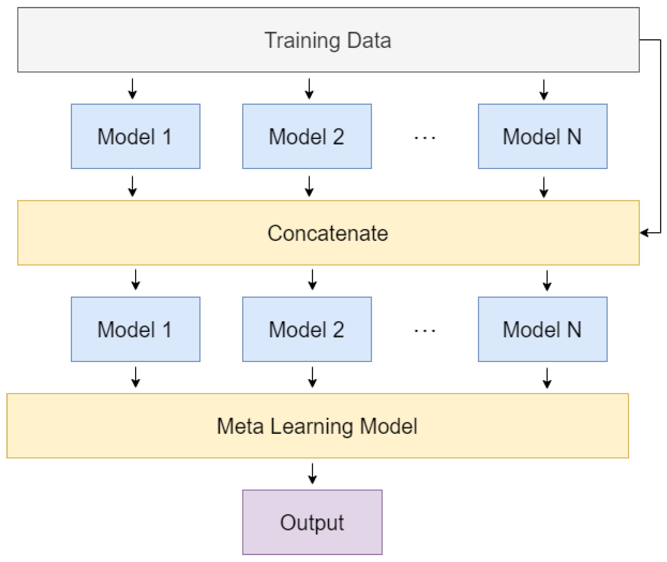
3.2.2. Development of Ensemble Learning Model

We applied the stacking ensemble learning package AutoGluon, which was developed by Amazon, to train the satellite-based estimation model [55]. The basic architecture of the multi-layer stack ensemble in AutoGluon is shown in Figure 3. In the model fitting step, the training data are first fed to multiple base models with different algorithms and structures, and the outputs of these base models are then concatenated with the training data via a meta-learning model. Then, multiple stacker models are trained on the outputs of the concatenation layers, such that these models share the same structures and hyperparameters as the base models. Finally, a meta-learning model is implemented to introduce these stacker models into a new ensemble model, thus optimizing its predictive accuracy. In addition, to mitigate model over-fitting and to further improve the predictive accuracy, AutoGluon repeats a k -fold cross-validation when fitting the model. In practice, we employed a five-fold cross-validation approach, in which the samples were randomly divided into five subsets of the same size. This process was conducted five times, with four subsets used for model training and one subset used for model validation in each replicated run.

AutoGluon enables automatic ensemble learning and leverages the hyperparameters tuned with state-of-the-art models by setting only a few parameters, such as the training data, time limits, and the bagging and multi-layer stack strategy. In this study, we used the random forest model, the CatBoost model, the XGBoost model, the LightGBM, and some NNs as the base models, and the weighted ensemble as the meta-learning model. In addition, we set the ’best_quality’ mode in ’auto_stack’ as True, which means that the model looks for the best accuracy without limiting the time, and we used a bagging strategy by automatically setting the number of bagging folds and the number of stacking levels.

3.2.3. Model Evaluation

A 10-fold cross-validation approach was used to evaluate the PM${}_{2.5}$ concentrations estimated by the ensemble learning model. This involved the random selection of 90% of the samples for use as training data, with the remaining 10% of the samples being used for testing. This procedure was conducted 10 times to cover the entire dataset. Additionally, the training data were validated using the fivefold cross-validation incorporated in AutoGluon, as aforementioned in Section 3.2.2.

3.3. Validation of Transferability of MIFNN Model

As the MIFNN model was trained on the PPCP dataset, it must be validated before being applied to another dataset, i.e., the SMP dataset. Furthermore, we first needed to retrieve the corresponding PM${}_{2.5}$ concentrations for all smartphone photographs in the SMP dataset; these data were obtained from the ground-based monitoring station closest to where each photograph was taken.

Given the accuracy of the PM${}_{2.5}$ concentrations measured by these ground-based monitoring stations, we regarded the smartphone photographs taken within 3 km of a given ground-based monitoring station as having the PM${}_{2.5}$ concentration measured at that monitoring station in the most recent hour. In practice, we first established a 3 km buffer around each ground-based monitoring station, and then selected the photographs taken within this buffer zone and within 30 min of the PM${}_{2.5}$ concentration release time as the validation data, using the PM${}_{2.5}$ concentration published by the closest monitoring station as the corresponding PM${}_{2.5}$ concentration. Figure 4 shows the result of validation data selection; all of these selected photographic data were used to validate the transferability of the MIFNN model to the SMP dataset.

4. Results

4.1. Evaluation of the MIFNN Model by Application to the PPCP Dataset

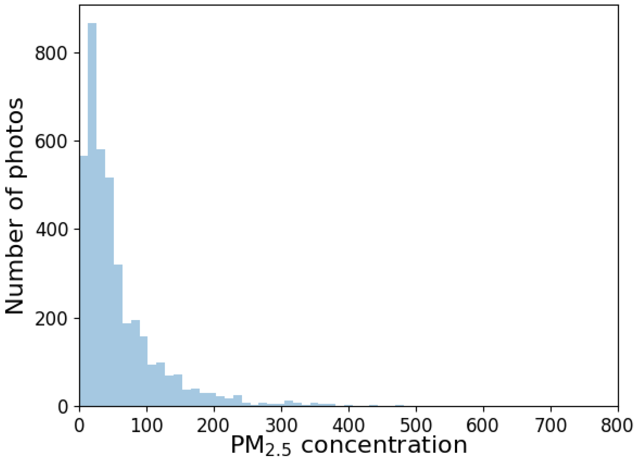
4.1.1. Ppcp Dataset

The PPCP dataset was created for training and validating the MIFNN model, and comprised two public smartphone photograph datasets shared by previous studies and one dataset that we generated. The latter dataset consisted of photographs taken with our smartphones in a range of locations and the corresponding PM${}_{2.5}$ concentrations, which we measured with a portable air-quality sensor. The PPCP dataset contained smartphone photographs of various scenes, such as buildings, lakes, roads, and mountains, but we excluded smartphone photographs taken on rainy or snowy days or at night, because the MIFNN model was designed to estimate the PM${}_{2.5}$ concentration in a smartphone photograph taken in clear weather during the daytime. In this study, the daytime photograph refers to a photograph that has high illumination intensity, where the illumination is contributed by the sunlight. This manual selection and exclusion process ultimately yielded a set of 4022 smartphone photographs with image resolutions ranging from 584 × 389 to 3124 × 4150 pixels. A histogram of the PM${}_{2.5}$ concentrations of these smartphone photographs is plotted in Figure 5.

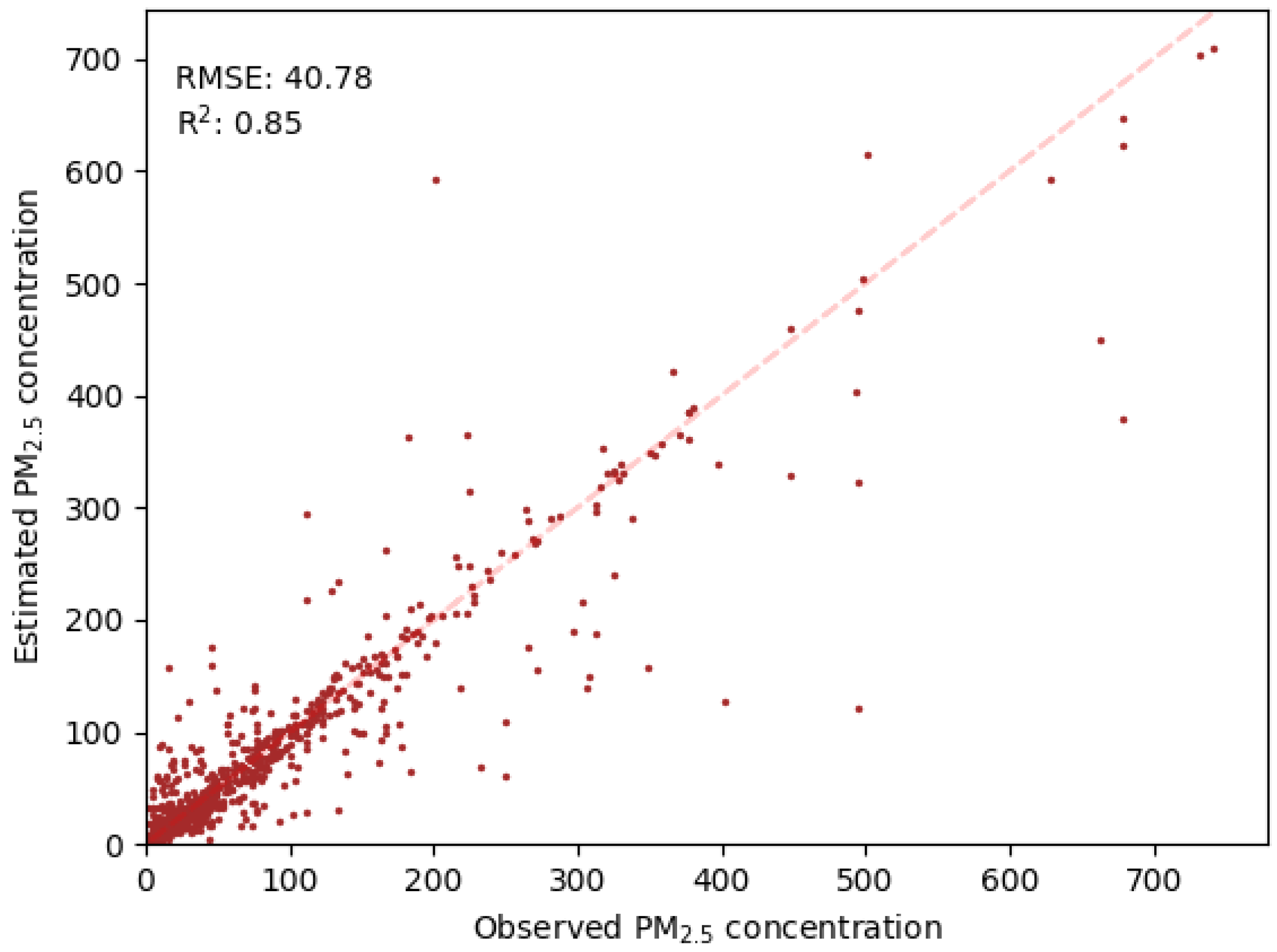
4.1.2. Performance of the MIFNN Model

As mentioned, during the model training and validation, the PPCP dataset was randomly divided into two parts: 80% of the dataset was used as the training data and the remaining 20% was used as the validation data. Additionally, image data augmentation was applied to scale up the training data; this involved rotating a photograph randomly between 0${}^{\circ }$ and 360${}^{\circ }$, flipping a photograph vertically or horizontally, or cropping or expanding a photograph to 4/5 or 5/4 of its original size, respectively.

Figure 6 illustrates the regression result for the entire validation dataset of 804 images. Figure 7 shows some example smartphone photographs with corresponding PM${}_{2.5}$ concentrations measured at ground-based monitoring stations and the PM${}_{2.5}$ concentrations estimated by the MIFNN model. It can be seen that the estimated PM${}_{2.5}$ concentrations correlate well with the PM${}_{2.5}$ concentrations measured at ground-based monitoring stations, with an RMSE of 40.78 µg/m${}^3$ and an R${}^2$ of 0.85.

To validate the effectiveness of using both physics-based features and CNN-based features in the MIFNN model, we also evaluated the performance of an NN model based only on physics features (a PFNN model) and that of an NN based only on CNN features (a CFNN model) applied to the PPCP dataset.

Table 3. Performance comparison of PFNN, CFNN, and MIFNN models.

Model	RMSE	R${}^2$
PFNN	70.34	0.32
CFNN	57.95	0.61
MIFNN	40.78	0.85

shows the experimental results, which reveal that the MIFNN model outperformed the PFNN and CFNN models. Specifically, the R${}^2$ of the MIFNN model was 0.53 and 0.24 greater than those of the PFNN and CFNN models, respectively, and the RMSE of the MIFNN model was 29.56 and 17.23 less than those of the PFNN and CFNN models, respectively. This comparison demonstrates that including multiple inputs, i.e., both photographic data and photographic feature data, can improve the accuracy of model estimations of PM${}_{2.5}$ concentrations.

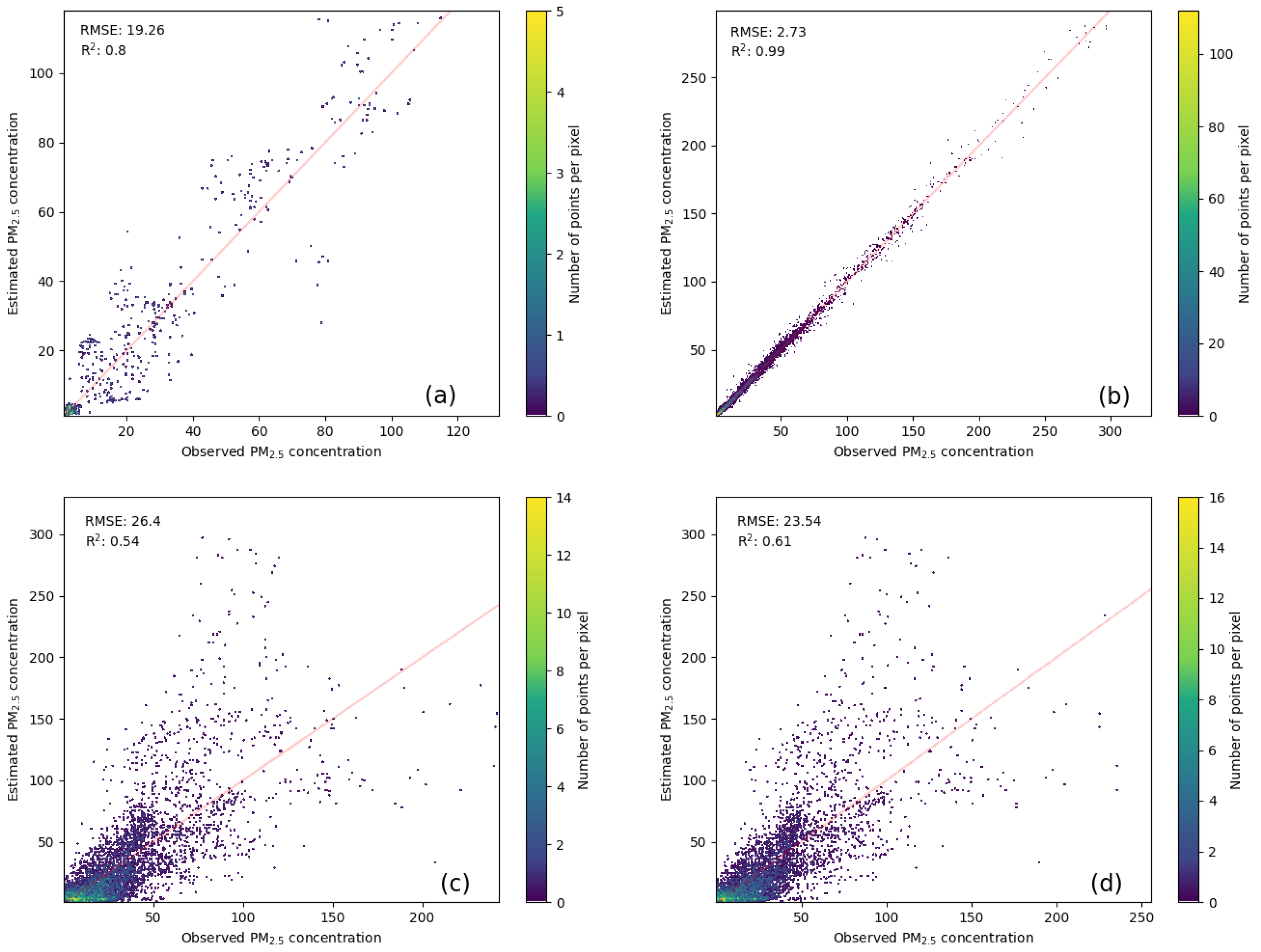
4.2. Evaluation of the AutoELM Model

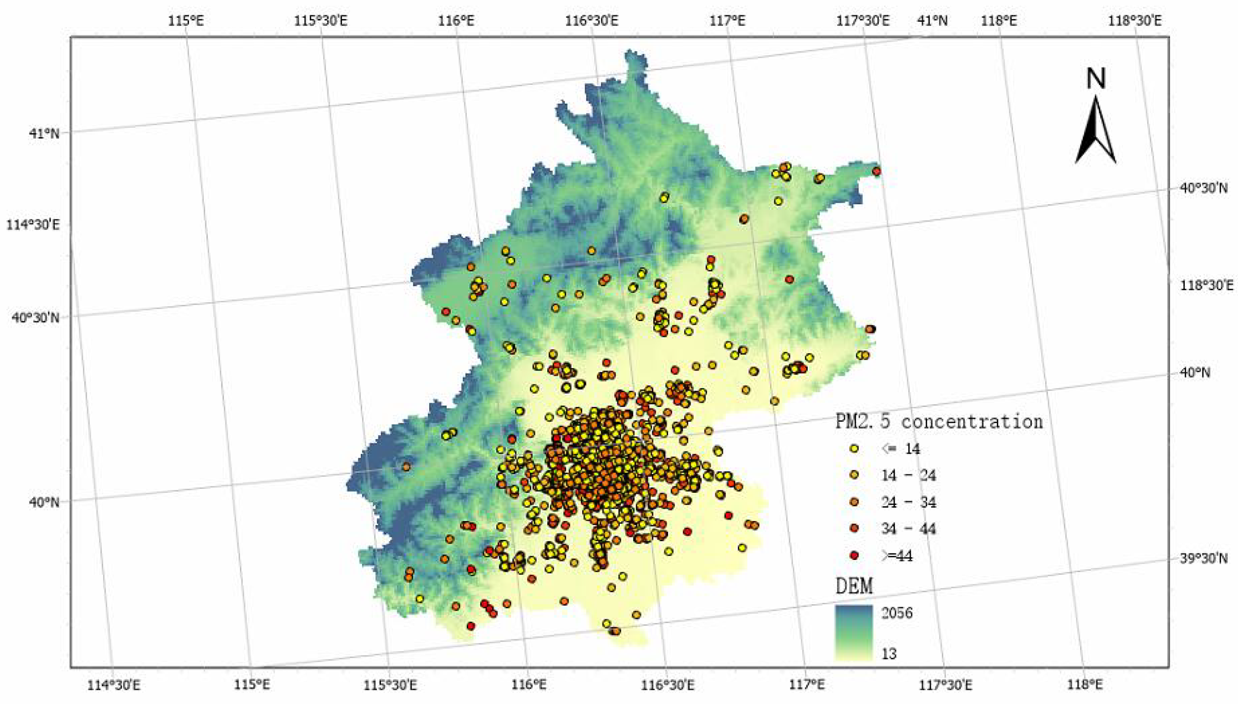
4.2.1. Descriptive Statistics

Table 4. Descriptive statistics of the data used in the AutoELM modeling.

Statistic	PM2.5	AOD	WS	TEMP	PS	RH	BLH	DEM	NDVI
Min	1.00	0.01	0.01	−6.88	92,745.69	0.09	231.54	18.00	0.02
Max	330.60	3.27	5.96	35.76	103,806.84	0.91	4006.09	493.00	0.85
Mean	31.94	0.37	1.61	17.30	99,741.07	0.37	1306.29	87.37	0.34
Median	18.20	0.22	1.31	17.15	100,001.89	0.34	1127.57	55.00	0.33
Std. Dev	38.97	0.38	1.22	9.35	1848.79	0.18	782.54	101.57	0.15

illustrates the summary statistics of the data that were collected in Beijing from 1 January 2021 to 31 December 2021, and which we used to fit the AutoELM model. To match these data with the MODIS AOD product, which only provides observations at approximately 10:30 a.m. and 1:30 p.m. local time, these hourly data from Beijing were averaged. Then, by comparing the averaged data with the MODIS AOD product, we obtained 4874 matches (see Section 2.2.5 for more details). Over the entire study area, the mean PM${}_{2.5}$ concentration was 31.94 µg/m${}^3$, which is well above the latest WHO annual average PM${}_{2.5}$ guideline (≤5 µg/m${}^3$). In addition, the PM${}_{2.5}$ concentration varies greatly throughout the year, with a maximum of 330.6 µg/m${}^3$, a minimum of 1 µg/m${}^3$, and a standard deviation of 38.97 µg/m${}^3$.

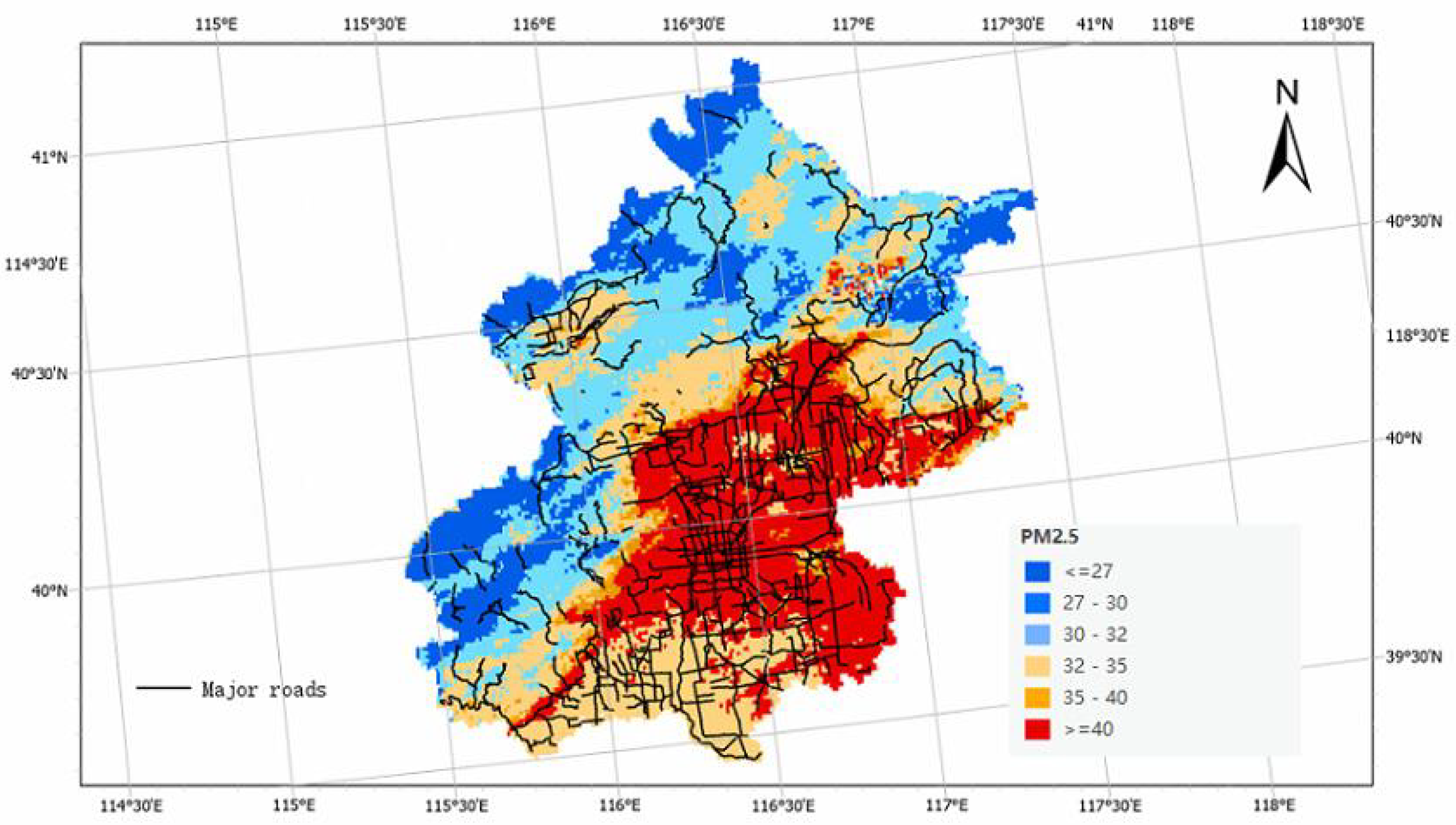
4.2.2. Model Performance and Estimates of PM${}_{2.5}$ Concentrations

Figure 8a,b shows the AutoELM performance, in terms of a comparison of PM${}_{2.5}$ concentrations measured at ground-based monitoring stations in Beijing during the stipulated period in 2021 and PM${}_{2.5}$ concentrations estimated during model training and model testing. In model training, the $R^2$ was 0.99 and the RMSE was 2.73 µg/m${}^3$, which suggest that the AutoELM generates good training approximations. In model testing, the $R^2$ was 0.80, indicating that the AutoELM can explain 80% of the variation in PM${}_{2.5}$ concentrations. Compared with the results of model training, the results of model testing suggest that the AutoELM somewhat overfit the data, as its $R^2$ was 0.19 lower and its RMSE was 16.53 µg/m${}^3$ higher. For comparison, we also estimated PM${}_{2.5}$ concentrations using an ordinary least squares (OLS) regression model and a GWR model, using the same 10-fold cross-validation approach. Figure 8c,d depicts the results of the OLS regression and the GWR. It can be seen that they achieved much worse accuracy than the AutoELM, as the $R^2$ of the OLS regression was 0.54 (0.26 less than that of the AutoELM) and the $R^2$ of the GWR was 0.61 (0.19 less than that of the AutoELM). This demonstrates that although the AutoELM overfits data during model training, its estimation capability is far superior to those of two traditional regression models. This is attributable to the AutoELM containing algorithms that detect nonlinear correlations and high-order interactions.

Figure 9 presents the annual mean PM${}_{2.5}$ concentrations in Beijing estimated by the AutoELM at a 1 km spatial resolution. There is strong spatial heterogeneity in the distribution of PM${}_{2.5}$ concentrations: high concentrations in densely populated urban areas and low concentrations in mountainous areas. In particular, the central urban areas and the southeastern suburban areas are the most polluted, with annual mean PM${}_{2.5}$ concentrations generally ranging from 32 to 40 µg/m${}^3$, but reaching higher than 40 µg/m${}^3$ in some areas of central Beijing, which are densely populated and have little vegetation. In contrast, the northern and western areas of Beijing are the least polluted, as they are mainly mountainous with lush vegetative cover and a sparse population; thus, their annual PM${}_{2.5}$ concentrations range from 27 to 32 µg/m${}^3$, decreasing to 27 µg/m${}^3$ in remote mountainous areas. Thus, these differences in PM${}_{2.5}$ concentrations between the northwestern and southeastern areas of Beijing are mainly due to variations in population density, vegetation cover, and topography. In addition to these internal factors, PM${}_{2.5}$ concentrations may also be influenced by external factors, such as the air pollution transported from Hebei province, which often affects the southern part of Beijing. Moreover, the solid black lines in Figure 9 represent the major roads in Beijing, which correspond well with the distribution of PM${}_{2.5}$; thus, PM${}_{2.5}$ concentrations are higher in urban areas with dense road networks than in mountainous areas with few or no road networks. These estimation results also show that the PM${}_{2.5}$ concentrations estimated from a combination of AOD and ancillary data are higher than those measured by ground-level PM${}_{2.5}$ monitoring stations. This is probably attributable to the fact that these monitoring stations are situated in remote or low traffic areas, such as scenic spots, mountains, or new towns, where PM${}_{2.5}$ concentrations are less than those in the urban surrounding areas.

4.3. Synergy of AOD-Based and Smartphone Photograph-Based Estimates of PM_2.5 Concentration

4.3.1. Transferability Validation

Following the methodology introduced in Section 3.3, we first created a 3 km buffer zone around PM${}_{2.5}$ monitoring stations (Figure 4), and then used the smartphone photographs taken within these buffer zones to verify the transferability of the MIFNN model to the new dataset (i.e., the SMP dataset). Figure 10 shows the estimates generated by the MIFNN model: the RMSE and R${}^2$ were 7.51 µg/m${}^3$ and 0.80, respectively, after validation with the PM${}_{2.5}$ concentrations measured at ground-level monitoring stations. The PM${}_{2.5}$ concentrations estimated by the MIFNN model when it was applied to the SMP dataset ranged from 3 to 58 µg/m${}^3$, which is much narrower than the range of PM${}_{2.5}$ concentrations estimated by the MIFNN model when it was applied to the PPCP dataset (1 µg/m${}^3$ to 770 µg/m${}^3$). Consequently, the RMSE of the MIFNN model applied to the SMP dataset was 7.51 µg/m${}^3$, much less than the RMSE of the MIFNN model applied to the PPCP dataset (40.78 µg/m${}^3$). Thus, despite the R${}^2$ of the SMP dataset being lower than that of the training dataset (the PPCP dataset), the R${}^2$ of 0.8 of the MIFNN model indicates that this model can explain 80% of the variation. This validates the reliability of the MIFNN model for estimating PM${}_{2.5}$ concentrations from the SMP dataset, which was downloaded from the Internet.

4.3.2. Fusion of Methods for the Estimation of PM_2.5 Concentrations

Figure 11 shows the distribution of all smartphone photographs taken in Beijing in November 2021 and downloaded from social media (these photographs are clustered mainly in the central area of the city), and their corresponding PM${}_{2.5}$ concentrations estimated by the MIFNN model. As the primary contributor to satellite-based PM${}_{2.5}$ concentration estimations is AOD data, the estimation result is frequently subject to missing values in AOD products, due to occlusion of satellite visibility by features such as pollution and clouds. For November 2021, the average ratio of days with AOD values to total days in Beijing is 0.60, with a minimum of 0.04 and a maximum of 0.79. This suggests that methods with AOD data as the primary predictor can only provide estimates of PM${}_{2.5}$ concentrations for this many days in Beijing in November 2021. However, after the fusion of AOD-based estimates with smartphone photograph-based estimates, the average ratio of days increases to 0.67 (an improvement of 12%), with a minimum of 0.04 and a maximum of 1.00. Figure 12 shows a comparison of the ratios before and after the introduction of smartphone photograph-based estimates for densely populated regions of Beijing. As can be seen, the mean ratio increases from 0.62 to 0.78, which is an improvement of 25%. We can infer from these comparisons that the combination of smartphone photograph-based estimates and AOD-based estimates can significantly increase the geographical coverage of estimations of PM${}_{2.5}$ concentrations, especially in densely populated areas (from which more smartphone photographs can be collected than from less densely populated areas). Moreover, it is more important to obtain estimates of PM${}_{2.5}$ concentrations in densely populated areas than in less densely populated areas, as the former contain more people who can potentially suffer adverse effects from exposure to PM${}_{2.5}$.

5. Discussion

5.1. Comparison with Previous Photograph-Based Methods for the Estimation of PM_2.5 Concentrations

As mentioned, photograph-based methods for the estimation of PM${}_{2.5}$ concentrations can be divided into two categories: image feature-based methods and NN-based methods. For comparison, we selected two state-of-the-art methods to estimate PM${}_{2.5}$ concentrations from the PPCP dataset; one method uses a model based on an image feature analysis algorithm [25], and the other method uses a model based on deep learning [35]. We implemented both methods according to the procedures described in their respective papers.

Table 5. Performance comparison of two selected models with that of the MIFNN model.

Model	RMSE	R${}^2$
Rijal et al. [35]	56.34	0.62
Liu et al. [25]	65.87	0.42
MIFNN	40.78	0.85

shows the results of these two methods and those generated by our MIFNN model.

Clearly, the MIFNN model exhibits better estimation performance than those of the two methods from the literature, as evidenced by their respective RMSEs and R${}^2$ values. Specifically, compared with the results generated by the method of Liu et al. [25] and the method of Rijal et al. [35], the RMSE of the results generated by the MIFNN model is 41.2% and 27.6% lower, respectively, and the R${}^2$ of the results of the MIFNN model is 37.1% and 102.3% higher, respectively.

Liu et al. [25] extracted seven image features via image analysis and used a support-vector regression model to study their correlations with PM${}_{2.5}$ concentrations. We did not consider weather conditions when applying this model. Liu et al. [25] found that this model performed well (an R${}^2$ of 0.57) when they applied it to a Shanghai dataset, because these photographs were taken at a fixed point, and the R${}^2$ for this model decreased with an increasing number of photographs taken at different scenes; this accounts for its generating results with an R${}^2$ of only 0.42 when we applied it to the PPCP dataset. In contrast, Rijal et al. [35] estimated PM${}_{2.5}$ concentrations based on an ensemble learning model that uses three CNNs as base models: VGG 16, Inception V3, and ResNet50. The accuracy of this model is approximately the same as that of our CFNN model (Table 3), with an R${}^2$ of 0.62, as they both take RGB channels of photographs as inputs and adopt a deep learning approach. Overall, these comparative experimental results suggest that deep learning-based methods are superior to image-feature-based methods when diverse outdoor scenes are included in a photographic dataset, and that incorporating both image data and image feature data into a model can improve its ability to accurately estimate PM${}_{2.5}$ concentrations, relative to that of a model incorporating only one type of data.

5.2. Comparison with Previous AOD-Based Methods for the Estimation of PM_2.5 Concentrations

We first compared the performance of the MIFNN model with that of the GTWR model of [56], who also used Beijing as their study area to estimate ground-level PM${}_{2.5}$ concentrations using satellite-derived AOD, meteorological, and land-use variables as predictors. The GTWR model generates results with a CV R${}^2$ of 0.69, which is significantly better than the performance of an OLS regression model and a GWR model (which generate results with an R${}^2$ of 0.54 and 0.61, respectively), because the GTWR model can account for spatiotemporal variability when learning the relationship. However, as our MIFNN model incorporates deep learning models to learn nonlinear correlations, it affords results with an even higher R${}^2$ (0.80).

In other previous studies, models have generated results with CV R${}^2$ values ranging from 0.71 to 0.84 [14,15,23], with these models having a similar predictive accuracy to the AutoELM. However, these studies used satellite AOD as their main predictor, which means that these models cannot provide estimates when AOD values are missing; i.e., these models are heavily affected by clouds and land cover. We solved this problem in this study by using smartphone photograph-based estimates of PM${}_{2.5}$ concentrations. As mentioned in Section 4.3.2, relative to models that use only AOD values, our MIFNN model increases the geographical area for which estimates of PM${}_{2.5}$ concentrations can be made by an average of 12%, which increases to 25% in densely populated areas.

5.3. Potential Limitations and Scope for Model Improvement

Despite these encouraging results, some aspects of our methods could be further improved. First, the MIFNN model can only be applied to smartphone photographs captured during the daytime in good weather, and photographs taken at nighttime or in rainy or snowy weather must be excluded. Thus, a model that is not limited by time or weather conditions should be developed. Second, there are few smartphone photographs on social media that have been taken in sparsely populated areas, and thus in future studies we will explore more websites to download additional smartphone photographs for generating finer-scale maps of estimated PM${}_{2.5}$ concentrations. Finally, we will explore more ancillary variables that affect in situ PM${}_{2.5}$ concentrations in future models, as this should improve the correlations between AOD and PM${}_{2.5}$ concentrations. These could include variables such as population, road networks, and emissions data.

6. Conclusions

In this study, we developed a novel method for estimating ground-level PM${}_{2.5}$ concentrations with high spatial coverage by integrating smartphone photograph-based estimations and satellite-based estimations. A fuzzy neural network with multiple inputs and an ensemble learning model stacking the random forest model, the CatBoost model, the XGBoost model, the LightGBM, and NNs were designed to estimate PM${}_{2.5}$ concentrations from smartphone photographs and satellite AOD data, respectively. Then, we fused the estimates generated by these two models to form a new PM${}_{2.5}$ distribution product with broader coverage than those that consider only AOD data. This achieved an average increase in the map coverage ratio (for estimates of PM${}_{2.5}$ concentrations) of 12% for the entire study area, rising to 25% in densely populated areas. Our novel method is an efficient and low-cost approach for acquiring real-time air quality data. Furthermore, it showcases the suitability of fusing smartphone photograph-based estimations and satellite-based estimations for solving low-coverage problems in large-area estimates of PM${}_{2.5}$ concentrations, which result from missing values in satellite AOD data.

References

1. Song, Y.; Chen, B.; Kwan, M.P. How does urban expansion impact people’s exposure to green environments? A comparative study of 290 Chinese cities. J. Clean. Prod. 2020, 246, 119018. [Google Scholar] [CrossRef]
2. Song, Y.; Chen, B.; Ho, H.C.; Kwan, M.P.; Liu, D.; Wang, F.; Wang, J.; Cai, J.; Li, X.; Xu, Y.; et al. Observed inequality in urban greenspace exposure in China. Environ. Int. 2021, 156, 106778. [Google Scholar] [CrossRef] [PubMed]
3. Franklin, M.; Koutrakis, P.; Schwartz, J. The role of particle composition on the association between PM2.5 and mortality. Epidemiology 2008, 19, 680. [Google Scholar] [CrossRef] [Green Version]
4. Song, Y.; Huang, B.; He, Q.; Chen, B.; Wei, J.; Mahmood, R. Dynamic assessment of PM2.5 exposure and health risk using remote sensing and geo-spatial big data. Environ. Pollut. 2019, 253, 288–296. [Google Scholar] [CrossRef] [PubMed]
5. Huang, F.; Pan, B.; Wu, J.; Chen, E.; Chen, L. Relationship between exposure to PM2.5 and lung cancer incidence and mortality: A meta-analysis. Oncotarget 2017, 8, 43322. [Google Scholar] [CrossRef] [PubMed] [Green Version]
6. Santibañez, D.A.; Ibarra, S.; Matus, P.; Seguel, R. A five-year study of particulate matter (PM2.5) and cerebrovascular diseases. Environ. Pollut. 2013, 181, 1–6. [Google Scholar]
7. Wang, C.; Tu, Y.; Yu, Z.; Lu, R. PM2.5 and cardiovascular diseases in the elderly: An overview. Int. J. Environ. Res. Public Health 2015, 12, 8187–8197. [Google Scholar] [CrossRef] [PubMed] [Green Version]
8. Xing, Y.; Xu, Y.; Shi, M.; Lian, Y. The impact of PM2.5 on the human respiratory system. J. Thorac. Dis. 2016, 8, E69. [Google Scholar] [PubMed]
9. Liu, P.; Zheng, J.; Li, Z.; Zhong, L.; Wang, X. Optimization of site locations of regional air quality monitoring network: Methodology study. China Environ. Sci. 2010, 30, 907–913. [Google Scholar]
10. You, W.; Zang, Z.; Pan, X.; Zhang, L.; Chen, D. Estimating PM2.5 in Xi’an, China using aerosol optical depth: A comparison between the MODIS and MISR retrieval models. Sci. Total Environ. 2015, 505, 1156–1165. [Google Scholar] [CrossRef] [PubMed]
11. Ma, Z.; Liu, Y.; Zhao, Q.; Liu, M.; Zhou, Y.; Bi, J. Satellite-derived high resolution PM2.5 concentrations in Yangtze River Delta Region of China using improved linear mixed effects model. Atmos. Environ. 2016, 133, 156–164. [Google Scholar] [CrossRef]
12. Lin, C.; Li, Y.; Yuan, Z.; Lau, A.K.; Li, C.; Fung, J.C. Using satellite remote sensing data to estimate the high-resolution distribution of ground-level PM2.5. Remote Sens. Environ. 2015, 156, 117–128. [Google Scholar] [CrossRef]
13. Guo, J.; Xia, F.; Zhang, Y.; Liu, H.; Li, J.; Lou, M.; He, J.; Yan, Y.; Wang, F.; Min, M.; et al. Impact of diurnal variability and meteorological factors on the PM2.5-AOD relationship: Implications for PM2.5 remote sensing. Environ. Pollut. 2017, 221, 94–104. [Google Scholar] [CrossRef] [PubMed] [Green Version]
14. He, Q.; Huang, B. Satellite-based mapping of daily high-resolution ground PM2.5 in China via space-time regression modeling. Remote Sens. Environ. 2018, 206, 72–83. [Google Scholar] [CrossRef]
15. Wei, J.; Huang, W.; Li, Z.; Xue, W.; Peng, Y.; Sun, L.; Cribb, M. Estimating 1-km-resolution PM2.5 concentrations across China using the space-time random forest approach. Remote Sens. Environ. 2019, 231, 111221. [Google Scholar] [CrossRef]
16. Geng, G.; Zhang, Q.; Martin, R.V.; van Donkelaar, A.; Huo, H.; Che, H.; Lin, J.; He, K. Estimating long-term PM2.5 concentrations in China using satellite-based aerosol optical depth and a chemical transport model. Remote Sens. Environ. 2015, 166, 262–270. [Google Scholar] [CrossRef]
17. Wu, J.; Yao, F.; Li, W.; Si, M. VIIRS-based remote sensing estimation of ground-level PM2.5 concentrations in Beijing–Tianjin–Hebei: A spatiotemporal statistical model. Remote Sens. Environ. 2016, 184, 316–328. [Google Scholar] [CrossRef]
18. Pang, J.; Liu, Z.; Wang, X.; Bresch, J.; Ban, J.; Chen, D.; Kim, J. Assimilating AOD retrievals from GOCI and VIIRS to forecast surface PM2.5 episodes over Eastern China. Atmos. Environ. 2018, 179, 288–304. [Google Scholar] [CrossRef]
19. Li, L.; Zhang, J.; Meng, X.; Fang, Y.; Ge, Y.; Wang, J.; Wang, C.; Wu, J.; Kan, H. Estimation of PM2.5 concentrations at a high spatiotemporal resolution using constrained mixed-effect bagging models with MAIAC aerosol optical depth. Remote Sens. Environ. 2018, 217, 573–586. [Google Scholar] [CrossRef]
20. He, Q.; Gu, Y.; Zhang, M. Spatiotemporal trends of PM2.5 concentrations in central China from 2003 to 2018 based on MAIAC-derived high-resolution data. Environ. Int. 2020, 137, 105536. [Google Scholar] [CrossRef] [PubMed]
21. Eeftens, M.; Beelen, R.; De Hoogh, K.; Bellander, T.; Cesaroni, G.; Cirach, M.; Declercq, C.; Dedele, A.; Dons, E.; De Nazelle, A.; et al. Development of land use regression models for PM2.5, PM2.5 absorbance, PM10 and PMcoarse in 20 European study areas; results of the ESCAPE project. Environ. Sci. Technol. 2012, 46, 11195–11205. [Google Scholar] [CrossRef] [PubMed]
22. Hu, X.; Waller, L.A.; Al-Hamdan, M.Z.; Crosson, W.L.; Estes, M.G., Jr.; Estes, S.M.; Quattrochi, D.A.; Sarnat, J.A.; Liu, Y. Estimating ground-level PM2.5 concentrations in the southeastern US using geographically weighted regression. Environ. Res. 2013, 121, 1–10. [Google Scholar] [CrossRef] [PubMed]
23. Park, Y.; Kwon, B.; Heo, J.; Hu, X.; Liu, Y.; Moon, T. Estimating PM2.5 concentration of the conterminous United States via interpretable convolutional neural networks. Environ. Pollut. 2020, 256, 113395. [Google Scholar] [CrossRef] [PubMed]
24. Feng, L.; Li, Y.; Wang, Y.; Du, Q. Estimating hourly and continuous ground-level PM2.5 concentrations using an ensemble learning algorithm: The ST-stacking model. Atmos. Environ. 2020, 223, 117242. [Google Scholar] [CrossRef]
25. Liu, C.; Tsow, F.; Zou, Y.; Tao, N. Particle pollution estimation based on image analysis. PLoS ONE 2016, 11, e0145955. [Google Scholar] [CrossRef]
26. Liu, X.; Song, Z.; Ngai, E.; Ma, J.; Wang, W. PM2.5 monitoring using images from smartphones in participatory sensing. In Proceedings of the 2015 IEEE Conference on Computer Communications Workshops (INFOCOM WKSHPS), Hong Kong, China, 26 April–1 May 2015; IEEE: Piscataway, NJ, USA, 2015; pp. 630–635. [Google Scholar]
27. Pudasaini, B.; Kanaparthi, M.; Scrimgeour, J.; Banerjee, N.; Mondal, S.; Skufca, J.; Dhaniyala, S. Estimating PM2.5 from photographs. Atmos. Environ. X 2020, 5, 100063. [Google Scholar] [CrossRef]
28. Gu, K.; Liu, H.; Xia, Z.; Qiao, J.; Lin, W.; Thalmann, D. PM2.5 Monitoring: Use Information Abundance Measurement and Wide and Deep Learning. IEEE Trans. Neural Netw. Learn. Syst. 2021, 32, 4278–4290. [Google Scholar] [CrossRef]
29. Liu, Y.; Racah, E.; Correa, J.; Khosrowshahi, A.; Lavers, D.; Kunkel, K.; Wehner, M.; Collins, W. Application of deep convolutional neural networks for detecting extreme weather in climate datasets. arXiv 2016, arXiv:1605.01156. [Google Scholar]
30. Qian, R.; Zhang, B.; Yue, Y.; Wang, Z.; Coenen, F. Robust Chinese traffic sign detection and recognition with deep convolutional neural network. In Proceedings of the 2015 11th International Conference on Natural Computation (ICNC), Zhangjiajie, China, 15–17 August 2015; IEEE: Piscataway, NJ, USA, 2015; pp. 791–796. [Google Scholar]
31. Yin, C.; Cheng, X.; Liu, X.; Zhao, M. Identification and classification of atmospheric particles based on SEM images using convolutional neural network with attention mechanism. Complexity 2020, 2020, 9673724. [Google Scholar] [CrossRef]
32. Zhang, C.; Yan, J.; Li, C.; Rui, X.; Liu, L.; Bie, R. On estimating air pollution from photos using convolutional neural network. In Proceedings of the 24th ACM International Conference on Multimedia, Amsterdam, The Netherlands, 15–19 October 2016; pp. 297–301. [Google Scholar]
33. Bo, Q.; Yang, W.; Rijal, N.; Xie, Y.; Feng, J.; Zhang, J. Particle pollution estimation from images using convolutional neural network and weather features. In Proceedings of the 2018 25th IEEE International Conference on Image Processing (ICIP), Athens, Greece, 7–10 October 2018; IEEE: Piscataway, NJ, USA, 2018; pp. 3433–3437. [Google Scholar]
34. Li, K.; Ma, J.; Li, H.; Han, Y.; Yue, X.; Chen, Z.; Yang, J. Discern Depth Under Foul Weather: Estimate PM2.5 for Depth Inference. IEEE Trans. Ind. Inform. 2019, 16, 3918–3927. [Google Scholar] [CrossRef]
35. Rijal, N.; Gutta, R.T.; Cao, T.; Lin, J.; Bo, Q.; Zhang, J. Ensemble of deep neural networks for estimating particulate matter from images. In Proceedings of the 2018 IEEE 3rd International Conference on Image, Vision and Computing (ICIVC), Chongqing, China, 27–29 July 2018; IEEE: Piscataway, NJ, USA, 2018; pp. 733–738. [Google Scholar]
36. Luo, Z.; Huang, F.; Liu, H. PM2.5 concentration estimation using convolutional neural network and gradient boosting machine. J. Environ. Sci. 2020, 98, 85–93. [Google Scholar] [CrossRef] [PubMed]
37. Qiao, J.; He, Z.; Du, S. Prediction of PM2.5 concentration based on weighted bagging and image contrast-sensitive features. Stoch. Environ. Res. Risk Assess. 2020, 34, 561–573. [Google Scholar] [CrossRef]
38. Dorogush, A.V.; Ershov, V.; Gulin, A. CatBoost: Gradient boosting with categorical features support. arXiv 2018, arXiv:1810.11363. [Google Scholar]
39. Chen, T.; Guestrin, C. Xgboost: A scalable tree boosting system. In Proceedings of the 22nd ACM Sigkdd International Conference on Knowledge Discovery and Data Mining, San Francisco, CA, USA, 13–17 August 2016; Association for Computing Machinery: New York, NY, USA, 2016; pp. 785–794. [Google Scholar]
40. Machado, M.R.; Karray, S.; de Sousa, I.T. LightGBM: An effective decision tree gradient boosting method to predict customer loyalty in the finance industry. In Proceedings of the 2019 14th International Conference on Computer Science & Education (ICCSE), Toronto, ON, Canada, 19–21 August 2019; IEEE: Piscataway, NJ, USA, 2019; pp. 1111–1116. [Google Scholar]
41. CSIS. Is Air Quality in China a Social Problem? 2021. Available online: https://chinapower.csis.org/air-quality/ (accessed on 14 February 2022).
42. Lyapustin, A.; Wang, Y.; Korkin, S.; Huang, D. MODIS collection 6 MAIAC algorithm. Atmos. Meas. Tech. 2018, 11, 5741–5765. [Google Scholar] [CrossRef] [Green Version]
43. Gu, K.; Qiao, J.; Li, X. Highly efficient picture-based prediction of PM2.5 concentration. IEEE Trans. Ind. Electron. 2019, 66, 3176–3184. [Google Scholar] [CrossRef]
44. McCartney, E.J. Optics of the Atmosphere: Scattering by Molecules and Particles. Phys. Today 1977, 30, 76. [Google Scholar] [CrossRef]
45. Narasimhan, S.G.; Nayar, S.K. Vision and the atmosphere. Int. J. Comput. Vis. 2002, 48, 233–254. [Google Scholar] [CrossRef]
46. Fattal, R. Single image dehazing. ACM Trans. Graph. (TOG) 2008, 27, 1–9. [Google Scholar] [CrossRef]
47. Koschmieder, H. Theorie der horizontalen Sichtweite. Beitr. Phys. Freien Atmos. 1924, 12, 33–53. [Google Scholar]
48. Swinehart, D.F. The beer-lambert law. J. Chem. Educ. 1962, 39, 333. [Google Scholar] [CrossRef]
49. Ozkaynak, H.; Schatz, A.D.; Thurston, G.D.; Isaacs, R.G.; Husar, R.B. Relationships between aerosol extinction coefficients derived from airport visual range observations and alternative measures of airborne particle mass. J. Air Pollut. Control. Assoc. 1985, 35, 1176–1185. [Google Scholar] [CrossRef]
50. He, K.; Sun, J.; Tang, X. Single image haze removal using dark channel prior. IEEE Trans. Pattern Anal. Mach. Intell. 2010, 33, 2341–2353. [Google Scholar] [PubMed]
51. Malm, W.C.; Leiker, K.K.; Molenar, J.V. Human perception of visual air quality. J. Air Pollut. Control Assoc. 1980, 30, 122–131. [Google Scholar] [CrossRef]
52. Szegedy, C.; Vanhoucke, V.; Ioffe, S.; Shlens, J.; Wojna, Z. Rethinking the inception architecture for computer vision. In Proceedings of the IEEE Conference on Computer Vision and Pattern Recognition, Las Vegas, NV, USA, 27–30 June 2016; pp. 2818–2826. [Google Scholar]
53. Zhou, S.; Li, W.; Qiao, J. Prediction of PM2.5 concentration based on recurrent fuzzy neural network. In Proceedings of the 2017 36th Chinese Control Conference (CCC), Dalian, China, 26–28 July 2017; IEEE: Piscataway, NJ, USA, 2017; pp. 3920–3924. [Google Scholar]
54. He, Z.; Ye, X.; Gu, K.; Qiao, J. Learn to predict PM2.5 concentration with image contrast-sensitive features. In Proceedings of the 2018 37th Chinese Control Conference (CCC), Wuhan, China, 25–27 July 2018; IEEE: Piscataway, NJ, USA, 2018; pp. 4102–4106. [Google Scholar]
55. Erickson, N.; Mueller, J.; Shirkov, A.; Zhang, H.; Larroy, P.; Li, M.; Smola, A. Autogluon-tabular: Robust and accurate automl for structured data. arXiv 2020, arXiv:2003.06505. [Google Scholar]
56. Guo, Y.; Tang, Q.; Gong, D.Y.; Zhang, Z. Estimating ground-level PM2.5 concentrations in Beijing using a satellite-based geographically and temporally weighted regression model. Remote Sens. Environ. 2017, 198, 140–149. [Google Scholar] [CrossRef]
Figure 1. Study area and spatial distribution of ground-level monitoring stations.
Remotesensing 14 01515 g001
Figure 2. A brief flowchart of our method.
Remotesensing 14 01515 g002
Figure 3. Multi-layer stack ensemble in AutoGluon.
Remotesensing 14 01515 g003
Figure 4. Three-kilometer buffers around monitoring stations and the locations at which smartphone photographs were taken.
Remotesensing 14 01515 g004
Figure 5. Histogram of PM 2.5 concentrations of the PPCP dataset.
Remotesensing 14 01515 g005
Figure 6. Correlation between PM 2.5 concentrations measured at ground-based monitoring stations and PM 2.5 concentrations estimated by the MIFNN model. The red dashed line is the 1:1 line.
Remotesensing 14 01515 g006
Figure 7. Examples of smartphone photographs with corresponding PM 2.5 concentrations measured at ground-based monitoring stations and PM 2.5 concentrations estimated by the MIFNN model.
Remotesensing 14 01515 g007
Figure 8. Density scatter plots of PM 2.5 concentrations measured at ground-based monitoring stations and PM 2.5 concentrations estimated by various methods. The data in (ad) are the testing data and training data for AutoELM, and the CV results of OLS regression and GWR, respectively. The red dashed lines represent the 1:1 line.
Remotesensing 14 01515 g008
Figure 9. Annual mean estimated PM 2.5 concentrations. The black lines are major roads in Beijing.
Remotesensing 14 01515 g009
Figure 10. Correlation between PM 2.5 concentrations measured by ground-based monitoring stations and those estimated by the MIFNN model. The red dashed line is the 1:1 line.
Remotesensing 14 01515 g010
Figure 11. Locations of smartphone photographs in Beijing obtained from social media in November 2021, with corresponding PM 2.5 concentrations estimated by the MIFNN model.
Remotesensing 14 01515 g011
Figure 12. Ratios of days with estimates of PM 2.5 concentrations to total days in densely populated regions, before (left) and after (right) the introduction of smartphone photograph-based estimates of PM 2.5 concentrations.
Remotesensing 14 01515 g012