Semantic Segmentation of Polarimetric SAR Image Based on Dual-Channel Multi-Size Fully Connected Convolutional Conditional Random Field

Abstract

The traditional fully connected convolutional conditional random field has a proven robust performance in post-processing semantic segmentation of SAR images. However, the current challenge is how to improve the richness of image features, thereby improving the accuracy of image segmentation. This paper proposes a polarization SAR image semantic segmentation method based on a dual-channel multi-size fully connected convolutional conditional random field. Firstly, the full-polarization SAR image and the corresponding optical image are input into the model at the same time, which can increase the richness of feature information. Secondly, multi-size input integrates image information of different sizes and models images of various sizes. Finally, the importance of features is introduced to determine the weights of polarized SAR images and optical images, and CRF is improved into a potential function so that the model can adaptively adjust the degree of influence of different image features on the segmentation effect. The experimental results show that the proposed method achieves the highest mean intersection over union (mIoU) and global accuracy (GA) with the least running time, which verifies the effectiveness of our method.

1. Introduction

Image semantic segmentation is used to generate a classification label for each pixel in an image, which is a fundamental technology in computer vision. Convolutional neural networks play an important role in the field of image segmentation. The Markov Random Field (MRF) model [1] is a classic model widely used in image segmentation. The MRF-based method performs segmentation from a statistical perspective. It constructs the joint distribution of the label field and the visual image under the Bayesian framework as a combination of likelihood and prior terms. Yiping Duan et al. proposed to use the Markov field model to realize the segmentation of polarized SAR images [2]. Nizar Bouhlel proposed an unsupervised image segmentation method for multi-view polarization synthetic aperture radar data, using the MRF model for pixel class labeling [3]. Conditional Random Field (CRF) adds an observation sequence based on MRF. CRF is an MRF under the condition of a given observation value, so the nature of CRF is the same as MRF to a certain extent. Fan Wang et al. proposed to use CRF for semantic segmentation of polarized SAR images [4]. Combining the powerful feature extraction capabilities of convolutional neural networks with the modeling capabilities of conditional random fields can make up for the shortcomings of neural networks that cannot make full use of context information. Due to its theoretical advantages [4], the CRF model has been widely used in various image processing tasks, such as image segmentation [5], land cover classification [6], hyperspectral image denoising [7], and multi-person target tracking [8].

The early post-processing of image semantic segmentation is mainly based on second-order CRF, which models the semantic information among different pixel categories in the four neighboring regions around the center pixel. This modeling method is limited to the short distance dependence between different pixels, and does not consider the semantic context relationship between the target categories of pixels whose spatial positions are far apart in the image. To solve the problem, Philipp Krähenbühl and Vladlen Koltun first proposed a fully connected CRF (FullCRF) [9]. The CRF of high-order potential functions realizes the long-distance dependence between pixels, but the computational complexity is very high, and the model reasoning is complicated. To solve this problem, Shuai Zheng [10] proposed a new form of the convolutional neural network, which combines the advantages of convolutional neural network and probabilistic graph modeling based on conditional random fields. The new form will have Gaussian pairwise potential. The approximate reasoning of the average field of the conditional random field is expressed as a recurrent neural network. This network is called CRF-RNN. MTT Teichmann et al. added a strong and effective conditional independence assumption to the framework of fully connected CRF, which allows the model to re-express most of the inference as convolution. This assumption can achieve a high degree of efficient use of a GPU, and this method is called convolutional CRF (convCRF) [11].

In recent years, many scholars have proposed a new semantic segmentation model based on convolution CRF. For example, Qiu Y proposed a semantic segmentation model based on multiple deep convolutional neural network (DCNN) models by employing convCRF [12]. However, due to the insufficient utilization of this fully connected convolutional CRF for image polarization information, the feature function template is relatively fixed, and the effect is still poor under the condition of low-resolution texture and scale information changes. Secondly, the existing fully connected convolution CRF is basically used for semantic post-processing of optical images. In order to achieve good performance of SAR images, it is necessary to conduct a deeper study on CRF. Moreover, most existing SAR image segmentation models are faced with the problem of insufficient feature information, which is also the core problem to be solved in this paper.

Based on a convolutional CRF, this paper proposes a polarization SAR image processing model based on dual-channel multi-size fully connected convolutional conditional random field, which further improves the fully connected convolutional dependent random field model for polarized SAR image segmentation performance. This paper uses a dual-channel model instead of a single-channel model, which can achieve similar effects while reducing model reasoning time. Then, inputting the corresponding optical image and polarized SAR image into the fully connected conditional random field at the same time, supplements the spectral information. Because images of different resolutions contain different information, multi-size input is used. The results of the random field output at different resolutions are weighted and summed, which further improves the semantic segmentation effect.

2. Literature Review

CRF is an MRF under a given observation value, so the nature of CRF is the same as MRF to a certain extent. According to the Hammersley–Clifford theorem, the joint probability distribution between several random variables contained in the MRF can be decomposed into the product of multiple individual factors through the cliques in the graph structure, where each element is only the largest one in the graph structure that is mission related [13]. Specifically, for the set of n observation variables $X=\{x_1,x_2,\dots ,x_n\}$ and label variables $Y=\{y_1,y_2,\dots ,y_n\}$, the set of all the largest cliques in the graph model is $C$, and the location of variables corresponding to the largest gang $Q\in C$ is $(y_Q,x_Q)$ so that the conditional probability distribution can be expressed as:

$$P(Y|X)=\frac{1}{Z}{\displaystyle \prod _{Q\in C}{\psi }_Q(y_Q,x_Q)}$$

(1)

$Z={\displaystyle \sum {\displaystyle \prod _{Q\in C}{\psi }_Q(y_Q,x_Q)}}$ is the normalization factor in ensuring that $P(Y|X)$ is a valid probability distribution.

This paper uses the CRF model to implement the post-processing of SAR image semantic segmentation. Assuming that the observation field $X$ is a random field corresponding to the set of random variables $x=\{x_1,x_2,\dots ,x_n\}$, corresponding to the SAR image to be semantically segmented, and $x_i$ represents the vector of the pixel $i$. $Y$ is the random field corresponding to the set of random variables $y=\{y_1,y_2,\dots ,y_n\}$, $y_i$ is the label vector corresponding to $x_i$, its value range is $L=\{l_1,l_2,\dots ,l_k\}$, and $k$ represents the total number of pixel categories to be semantically segmented in the image. Thus, the conditional random field $(X,Y)$ can be, based on the Gibbs distribution, expressed as:

$$P(Y|X)=\frac{1}{Z(X)}\exp (-{\displaystyle \sum _{c\in C_g}{\varphi }_c}(y_c|X))$$

(2)

$g=(V,\epsilon )$ is a graph model defined on $Y$, and a potential energy function ${\varphi }_c$ is introduced for each group $C_g$ in the group in the graph $g$ [13]. Therefore, the Gibbs energy corresponding to the label vector set $y\in L^n$ is:

$$E(y|X)=-\ln (P(y|X))-\ln (Z(X))={\displaystyle \sum _{c\in C_g}{\varphi }_c(y_c|X)}$$

(3)

Therefore, the goal of the corresponding CRF is to determine a label $y^{\ast }$ under the given input $X$ condition so that the posterior probability preaches the maximum value, and the related Gibbs energy E is the minimum at this time, namely:

$$y^{\ast }=\underset{\gamma }{\arg \max }P(y|X)=\underset{\gamma }{\arg \min }E(y|X)$$

(4)

In the densely connected CRF, $g=(V,\epsilon )$ is the complete graph model of $Y$, and $C_g$ represents the uni-group and binary group in the graph model. Therefore, the corresponding Gibbs energy can be expressed as:

$$E(y|X)={\displaystyle \sum _{i\in n}{\varphi }_i(y_i|X)}+{\displaystyle \sum _{i\in n,j\in {\delta }_i}{\varphi }_p(y_i,y_j|X)}$$

(5)

where ${\delta }_i$ represents the neighborhood of pixel $i$, the unary potential function ${\varphi }_i(y_i|X)$ is only related to the information contained in a single element itself. The binary potential function ${\varphi }_p(y_i,y_j|X)$ represents the semantic relationship between different label categories in the image, which can be expressed by the linear combination of the Gaussian kernel function $k^{(m)}$ defined in the feature space as:

$${\varphi }_p(y_i,y_j|X)=\mu (y_i,y_j){\displaystyle \sum _{m=1}^k{w}^{(m)}{k}^{(m)}(f_i-f_j)}$$

(6)

where ${\mu }^{(m)}$ is the tag compatibility function, which indicates the possibility of two different tag categories appearing in the same adjacent area, such as theoretically tag {boat} and tag {water}, then tag {bird} and tag {water}, appearing in the same neighborhoods are more likely.

3. Method

3.1. Network Mode

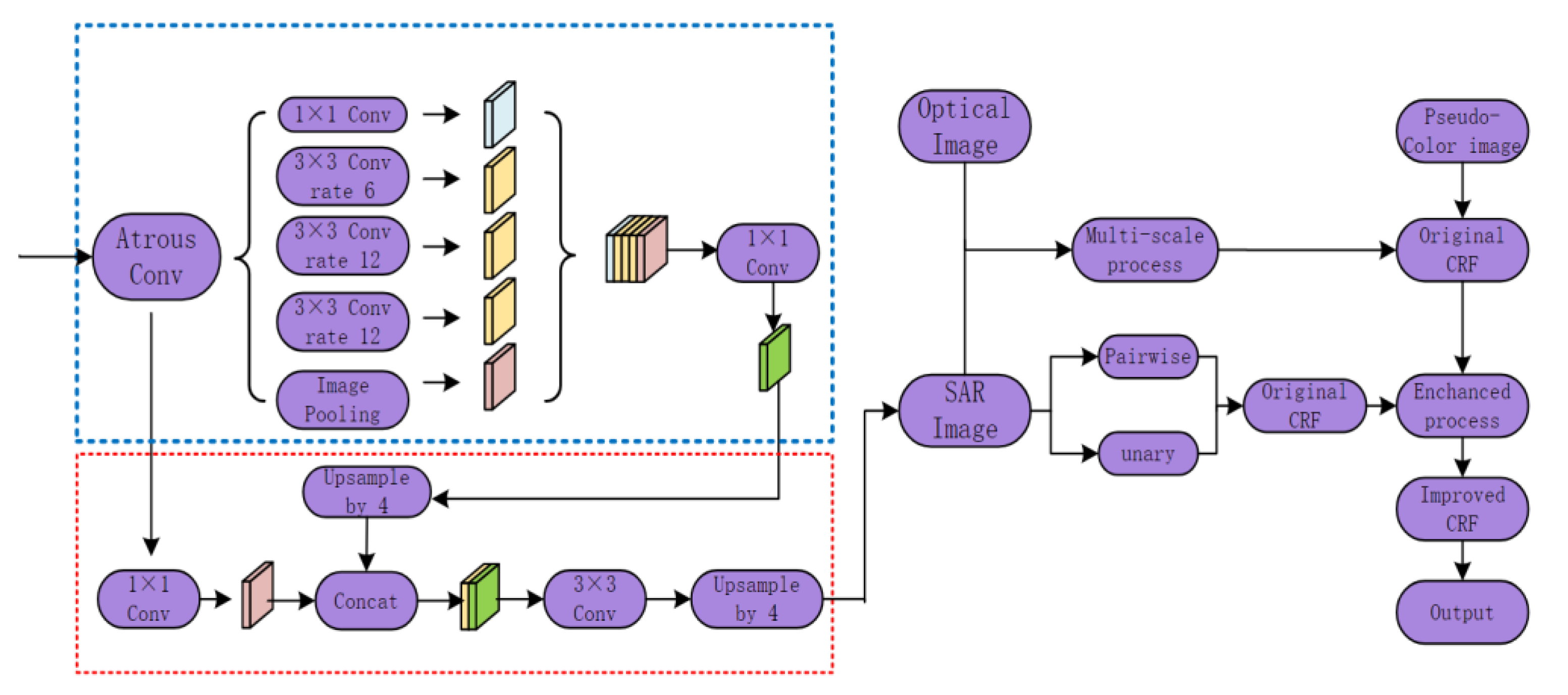
In this paper, the polarimetric SAR image and the corresponding optical image are simultaneously input into the fully connected random field model. The structure of the entire model is shown in Figure 1. As can be seen from the figure, the unary potential function of the fully connected conditional random field still models the semantic segmentation results of polarimetric SAR image outputs by the previous DCNN. Through the input of optical image, more abundant feature information is introduced into the energy function, such as the spatial feature and spectral feature of pixels. More context exists between adjacent pixel categories in the image can be captured during the overall conditional random field modeling process—semantic dependencies.

According to the fully connected conditional random field model, for the convenience of reading and writing, the condition X is omitted, and the unary potential function and the binary potential function are respectively expressed as:

$${\displaystyle \sum _{i\in n}{\varphi }_i(y_i)}=-\log p(y_i)$$

(7)

$${\varphi }_{i,j}(y_i,y_j)={\displaystyle \sum _{m=1}^K{\mu }_m(y_i,y_j)w_m\exp (-{\alpha }_m|f_i-f_j{|}^2)}$$

(8)

where $p(y_i)$ represents the predicted probability value of the ith pixel category output by DCNN, ${\mu }_m(y_i,y_j)$ represents the label compatibility function, and $f_i$ represents the feature vector of the ith pixel category. It can be seen that the unary potential function is based on the semantic segmentation results of polarimetric SAR images output by the previous deep convolutional neural network. In contrast, the binary potential function utilizes the spectral feature information of optical images, which can further improve the semantic segmentation effect. The fully polarimetric pseudocolor SAR image can further display the image features of the polarimetric SAR image. Using it as the auxiliary input of the optical image in the dual-channel model can significantly expand the detailed information of the image. The binary potential function expression of the polarimetric SAR image and the optical image is:

$${\varphi }_p(y_i,y_j)={\lambda }_{optical}[{\varphi }_{optical}(y_i,y_j)+{\varphi }_{colour}(y_i,y_j)]+{\lambda }_{SAR}{\varphi }_{SAR}(y_i,y_j)$$

(9)

${\varphi }_{optial}(y_i,y_j)$, ${\varphi }_{SAR}(y_i,y_j)$ and ${\varphi }_{colour}(y_i,y_j)$ represent the potential binary functions established by the optical image, polarimetric SAR image, and full polarimetric pseudo-color SAR image, respectively, ${\lambda }_{optical}$ and ${\lambda }_{SAR}$ represent the corresponding weighting coefficients.

The binary potential function corresponding to the optical image is composed of the feature $I$ and the position $p$:

$${\varphi }_{optical}(y_i,y_j)=\mu (y_i,y_j)\{w_1\exp (-\frac{{\left|p_i-p_j\right|}^2}{2{\theta }_{\gamma }^2})+w_2\exp (-\frac{{\left|p_i-p_j\right|}^2}{2{\theta }_{\alpha }^2}-\frac{{\left|I_i-I_j\right|}^2}{2{\theta }_{\beta }^2})\}$$

(10)

The first term indicates that two pixels closer together are more likely to belong to the same pixel label, and the second term indicates that two pixels with similar locations and features are more likely to belong to the same class. Feature I of the optical image consists of two aspects: (1) The R, G, and B channels are the three features of the spectral feature; and (2) based on the gray value of the image, the potential spatial relationship information is converted into texture information, such as variance, energy, and other features.

The binary potential function corresponding to the polarimetric SAR image is composed of the feature $f$ and the position $p$:

$${\varphi }_{SAR}(y_i,y_j)=\mu (y_i,y_j)\{w_1\exp (-\frac{{\left|p_i-p_j\right|}^2}{2{\theta }_{\gamma }^2})+w_2\exp (-\frac{{\left|p_i-p_j\right|}^2}{2{\theta }_{\alpha }^2}-\frac{{\left|f_i-f_j\right|}^2}{2{\theta }_{\beta }^2})\}$$

(11)

The feature $f$ of the polarimetric SAR image is extracted by Pauli decomposition, Freeman decomposition, Yamaguchi decomposition, and correlation feature decomposition of polarimetric features.

The label compatibility function $\mu (y_i,y_j)$ represents the probability of two different superpixel categories appearing simultaneously in adjacent positions. One of the most straightforward label compatibility functions is the Potts model:

$$\mu (y_i,y_j)=\{\begin{array}{l}0{,}^{}if\begin{array}{c}\end{array}{y}_i=y_j\\ 1{,}^{}others\end{array}$$

(12)

The Potts model imposes the same penalty on all inconsistent pixel labels in the image, but in practice, the network should implement different penalties. This section uses the method of [13] to implement the label compatibility function in the model inference process of learning.

In summary, the two-channel multi-scale fully connected convolutional conditional random field is expressed as the weighted sum of the input CRF output results of different resolution images:

$$E^{\ast }(y)={\displaystyle \sum _s{\lambda }_s{E}_s(y)}$$

(13)

Among them, ${\lambda }_s$ represents the weight value corresponding to the input of polarimetric SAR images of different sizes.

3.2. Polarimetric SAR Image and Optical Image Weight Parameter Estimation

Feature screening experiments are performed. This experiment determines the importance of different features of polarimetric SAR images and optical images for the final processing results. The weighting coefficients ${\lambda }_{SAR}$ and ${\lambda }_{optical}$ of the polarimetric SAR image and the optical image in the binary potential function are determined according to the proportion of feature importance. For this reason, this section takes polarimetric SAR images and optical images as research data and studies the importance of features, and obtains the results. In order to find the optimal value of the weighting coefficients ${\lambda }_{SAR}$ and ${\lambda }_{optical}$ of the binary potential functions ${\varphi }_{SAR}(y_i,y_j)$ and ${\varphi }_{optial}(y_i,y_j)$ of the polarimetric SAR image and the optical image in Formula (9), this section uses the support vector machine feature recursive elimination (SVM-RFE) method. In this section, a total of 32 optical image features and polarimetric SAR image features are extracted first, and then the SVM-RFE method is used to screen and sort the 32 features.

The first step is optical image feature extraction. The optical image mainly adopts the technology of spectral feature and texture feature extraction, in which the spectral feature uses the R, G, B channels of the optical image as the three vectors of the spectral feature, and the texture feature is based on the gray value of the image. The relationship information is converted into texture information, and the mean, variance, energy, etc., are all commonly used feature indicators. First of all, this paper uses the R, G, B channels of the optical image as the three eigenvectors of the spectral features, which are expressed as:

$$I_1={[I^1,I^2,I^3]}^T={[I^R,I^G,I^B]}^T$$

(14)

Secondly, the co-occurrence grayscale matrix is used to extract features. This paper extracts eight kinds of texture information as feature vectors, namely: mean, energy, variance, homogeneity, entropy, correlation, contrast, and dissimilarity, are expressed as:

$$I_2={[I^4,I^5,I^6,I^7,I^8,I^9,I^{10},I^{11}]}^T$$

(15)

The second step is feature extraction of polarimetric SAR images. Polarimetric SAR images mainly use polarimetric decomposition algorithms, such as Pauli decomposition, H/A/α decomposition, Freeman decomposition, Yamaguchi decomposition, and polarimetric feature correlation feature decomposition.

Pauli decomposition principle is relatively basic, based on a polarization scattering matrix, which is the sum of certain scattering mechanism matrices, and can be expressed as:

$$f_3=[f^{12},f^{13},f^{14}]=\frac{1}{\sqrt{2}}{[S_{HH}+S_{VV},S_{HH}-S_{VV},2S_{HV}]}^T$$

(16)

The H/A/α decomposition is the eigendecomposition of the scattering correlation matrix and three eigenvectors, the average scattering angle α, the scattering entropy H, and the anisotropy A, are extracted. Where A is anisotropy, which can provide information about the distribution of eigenvalues, when the H value is significant, it can indicate the degree of influence of the second and third largest scattering mechanism eigenvalues on the results. The three extracted feature vectors are:

$$f_4={[f^{15},f^{16},f^{17}]}^T={[f^A,f^H,f^{\alpha }]}^T$$

(17)

Freeman decomposition is a commonly used incoherent target decomposition method in this paper to obtain three distinct polarization components of plane scattering power, dihedral angle scattering power, and volume scattering power. The main idea of Freeman decomposition is based on the assumption of reflection symmetry. The correlation coefficient between co-polarization and cross-polarization is 0, and each pixel is composed of three types of scattering; that is, a first-order Bragg surface scattering. The surface scattering component of the even reflection component was obtained from the dihedral corner reflector, and the volume scattering component was obtained from a series of directional dipole scattering from the vegetation canopy [14]. Freeman decomposition is based on the C matrix, and three eigenvectors of even scattering, volume scattering, and surface scattering are extracted by calculation, respectively expressed as:

$$f_5={[f^{18},f^{19},f^{20}]}^T={[f^{Pd},f^{Ps},f^{Py}]}^T$$

(18)

The Yamaguchi decomposition can generally be cited not only in the case of asymmetric reflection, but also in the case of reflection symmetry. Compared with the Freeman decomposition based on reflection symmetry, Yamaguchi is more universal and used in a broader range [15]. The Yamaguchi decomposition extends the Freeman decomposition as it used the same even and surface scattering components. It modifies the bulk scattering component by changing the probability density function of the associated azimuth while adding a new component, the helix scattering component, which is suitable for more complex areas in urban buildings. The four feature vectors extracted by Yamaguchi decomposition can be expressed as:

$$f_6={[f^{21},f^{22},f^{23},f^{24}]}^T={[f^{Pd},f^{Ps},f^{Py},f^{Ph}]}^T$$

(19)

Surface objects generally appear as complex mixtures of different standard scatterers or standard targets, and the polarization characteristics of standard targets should be used as a reference for classification. The polarization characteristic map reflects the change of the radar received power of the target under different polarization modes to a certain extent and can be used to analyze the polarization characteristics of different targets so different types of ground objects can be distinguished. Usually, the characteristic polarization map can be used to analyze and describe the effect of calibration accuracy on the polarization scattering characteristics of the target. In this paper, PSCF decomposition mainly extracts four kinds of radar polarization features of dihedral angle, flat plate, horizontal dipole, and vertical dipole and calculates the correlation coefficient:

$$CQ=\frac{S_1}{S_2{S}_3}$$

(20)

Among them, $S_2$ represents the standard deviation of the polarization characteristics of the observed image pixels, $S_3$ represents the standard deviation of the polarization characteristics of the standard target, and $S_1$ represents the covariance between the standard target and the image pixels.

Using the above formula, the feature correlation coefficient between a single target and four standard target tables can be established, and a total of 8 feature vectors can be obtained, which are co_DI, co_FP, co_HD, co_VD, cross_DI, cross_FP, cross_HD, cross_VD, and co is the same polarity, the cross is cross-polarized:

$$\begin{array}{l}{f}_7={[f^{25},f^{26},f^{27},f^{28},f^{29},f^{30},f^{31},f^{32}]}^T\\ ={[f^{co\_DI},f^{co\_FP},f^{co\_HD},f^{co\_VD},f^{cross\_DI},f^{cross\_FP},f^{cross\_HD},f^{cross\_VD}]}^T\end{array}$$

(21)

The third step is feature screening. In terms of feature screening, this section adopts sensitivity analysis. First, the sensitivity is calculated for each feature through measurement indicators, and the cross-validation method is used to analyze its impact on subsequent processing. Then, using SVM-RFE to train the filtered feature set, calculating the importance of each feature and sorting them, deleting the features with the minor importance, obtains the optimal feature subset, and calculating the accuracy rate through the training model ensures the accuracy of deletion. It is the least important feature. Feature sensitivity mainly refers to the effect and influence of each feature value on the system to different degrees. The main sensitivity measures used are: input the extracted high-dimensional feature vector set, combine the cross-validation method to calculate the sensitivity of each feature according to the sensitivity measurement standard, and delete the feature vector with less contribution or less impact.

Calculate the variation range $Q_r$ of the system response when the eigenvalue changes. The nth eigenvalue is $x_n$, and its value range is divided into M equals, where the ith value is $x_{n_i}$, and the response is $y_{n_i}$, then the variation range $Q_{nr}$ of the nth feature is:

$$Q_{nr}=y_{n\max }-y_{n\min }$$

(22)

Calculate the change $Q_{nv}$ at the output when the eigenvalues of the input change:

$$Q_{nv}=\frac{{\displaystyle \sum _{i=1}^N\left|y_{n_i}-y_{pavg}\right|}}{N}$$

(23)

where $y_{pavg}$ is the average value.

Calculate the gradient value $Q_{ng}$ of all adjacent points:

$$Q_{ng}={\displaystyle \sum _{i=1}^N\left|\frac{y_{n_{i+1}}-y_{n_i}}{x_{n_{i+1}}-x_{n_i}}\right|}$$

(24)

By calculating the sensitivity of the eigenvalues, the eigenvectors with less contribution or less influence are deleted.

SVM is a further developed classification algorithm based on statistical learning and optimization theories. Its operation process is shown in Figure 2. It can only be applied to deal with classification and regression problems in nonlinear, high-level data modes with small samples [13]. Assuming that $x_i$ and $y_i$ are the ith samples in the training set, N is the sample size, and D is the number of sample features. SVM seeks the optimal classification hyperplane:

$$wx+b=0$$

(25)

Objective function:

$$L=\min \frac{1}{2}{\Vert w\Vert }^2$$

(26)

Restrictions:

$$y_i(wx+b)\ge 1$$

(27)

I = 1,2,…,N

(28)

$$y\in \left\{-1,1\right\}$$

(29)

Among them, w is the weight vector, x is the input feature vector, b is the deviation value, and the purpose is to make the variable target minimum; that is, the maximum geometric interval. The original problem can be transformed into a dual problem:

$$L=\min \frac{1}{2}{\displaystyle \sum _{i=1}^N{\displaystyle \sum _{j=1}^N{\alpha }_i{\alpha }_j}}{y}_i{y}_j(x_i·x_j)-{\displaystyle \sum _{i=1}^N{\alpha }_i}$$

(30)

Among them, ${\alpha }_i$ is the Lagrange multiplier, and the final solution is:

$$w={\displaystyle \sum _{i=1}^N{\alpha }_i{x}_i{y}_i}$$

(31)

Then the optimal decision can be expressed as:

$${\displaystyle \sum _{i=1}^N{\alpha }_i{x}_i{y}_i}+b=0$$

(32)

The formula for calculating the importance of the ith feature is:

$$C_i=w_i^2$$

(33)

Finally, the weighting coefficients ${\lambda }_{optical}$ and ${\lambda }_{SAR}$ of the binary potential function of the polarimetric SAR image and the optical image are obtained as:

$${\lambda }_{SAR}=\frac{{\displaystyle \sum _{i=1}^{11}{C}_i}}{{\displaystyle \sum _{i=1}^{32}{C}_i}}$$

(34)

$${\lambda }_{optical}=\frac{{\displaystyle \sum _{i=12}^{32}{C}_i}}{{\displaystyle \sum _{i=1}^{32}{C}_i}}$$

(35)

In each round of training, the extracted 32 features are selected for training, and then the classification hyperplane is obtained. For 32 features, SVM-RFE will delete the corresponding feature of the sequence number with the smallest square value of the component in w; in the second round, the number of features will be reduced by one, and continue to use the remaining features to train the same, removing the least important feature.

4. Results

This paper uses the full-polarization SAR data collected by the radars at 2 satellite in Nanjing city and surrounding areas, with four polarization states: HH, VV, HV, and VH. The data were acquired on 19 April 2011, with a resolution of 8 m. The optical image resolution was 5 m, and the acquisition time was April 2017. These images have an incident angle of 26°42′55″ with azimuth resolution of 4.74 m and range-direction resolution of 4.73 m. The images are 256 × 256 pixels in size, and include rivers, buildings, mountains, and roads. The architective area occupies the majority of the image, the vegetation area is relatively concentrated, and there is a small amount of vegetation within the building space. The cultivated area is concentrated in the northern part of the river. A clear color difference can be observed in the optical image between the dense vegetation area and the cultivated area. The color of the river part is not sufficiently uniform, which is similar to the farmland in some areas. In contrast, the river area of the SAR false-color image is different from other regions. Therefore, it can be seen that polarized SAR has apparent advantages in identifying river categories. The full-polarization SAR data are first subjected to pseudo-color fusion processing, and then data enhancement operations, such as random rotation mirroring, are performed. Finally, the initial 1000 SAR images are expanded to 2000 and divided into training set 1800 and validation set 200.

Before the experiment, the parameter settings of the model were first introduced. Then the initial CRF, convolutional CRF, and the improved dual-channel multi-size convolutional CRF were tested, respectively. Then the performance of the three models was tested. After analysis, the semantic segmentation results post-processed by the three models were compared with the semantic segmentation results obtained by the direct output of the original network. Finally, the full-polarization pseudo-color image was input to the improved dual-channel multi-scale convolutional CRF for testing. The segmentation results of the single-polarization image are compared.

In the experiment, in order to prove the effectiveness of the dual-channel multi-size convolutional CRF proposed here, the parameter settings in the model are the same as those in the reference paper, that is, $w_1=w_2={\theta }_{\gamma }=1$, ${\theta }_{\alpha }={\theta }_{\beta }=13$, and because the convolutional CRF uses the conditional independence assumption, the final accuracy of the entire model is related to the filter kernel parameter $k$, which is set to be the same as the setting of the paper [14]. The average approximate inference of the fully connected CRF of five iterations was performed in all experiments. The experiment was implemented in a Linux system with RTX 2080 Ti GPU, mainly using Python programming language and PyTorch deep learning framework.

4.1. Feature Importance Ranking Experimental Results

In this section, we first use the Support Vector Machine Feature Recursive Elimination (SVM-RFE) method for feature screening to obtain the estimated values of the parameters ${\lambda }_{optical}$ and ${\lambda }_{SAR}$ of Formula (9).

The characteristics of the method used in this paper mainly use the overall accuracy (OA), kappa coefficient (Kappa), recall rate (recall), accurate rate (precision) and f1-score parameter (F1) as the parameter indicator of the performance of the objective evaluation characteristics.

The overall accuracy is one of the important indicators. Overall accuracy is:

$$\mathrm{OA}=\frac{TP+TN}{TP+TN+FP+FN}$$

(36)

Precision is a very important indicator, which means that the proportion of the positive examples of the positive cases are divided into the positive example. The precision rate is:

$$\mathrm{precision}=\frac{TP}{TP+FP}$$

(37)

Recall rates are divided into positive cases, and the recall rate is:

$$\mathrm{recall}=\frac{TP}{TP+FN}$$

(38)

The kappa coefficient is an important method of statistical evaluation consistency, which is generally evaluated by 0, 1. The higher the kappa coefficient, the better the selection performance, the kappa coefficient is expressed as:

$$\mathrm{Kappa}=\frac{\mathrm{OA}-P_e}{1-P_e}$$

(39)

$$P_e=\frac{a_1{b}_1+a_2{b}_2+\mathrm{\dots }{a}_N{b}_N}{N^2}$$

(40)

In this case, $a_i$ is the real sample number of the i class, and $b_i$ represents the number of the sample of the i. N represents the total number of samples.

F1-score is a harmonic average of accuracy and recall rate, which can be used in a certain type of class to identify the comprehensive energy of accuracy and recall, so it is often used in machine learning competitions to determine the final evaluation index. The maximum value is 1, the minimum is 0.

$$F1=2\times \frac{precision\times recall}{precision+recall}$$

(41)

Of these, the group FN, FP, TN, are all a confused matrix; the positive example of the prediction is that all the samples in the actual case are called the real (TP). The positive example of the prediction is that all the samples in the actual case are called false (FP); in the prediction, all the samples of the positive case in practice are called false cases (FN); the inverse example of the prediction is that all samples of the counterexample are called the true reverse case (TN).

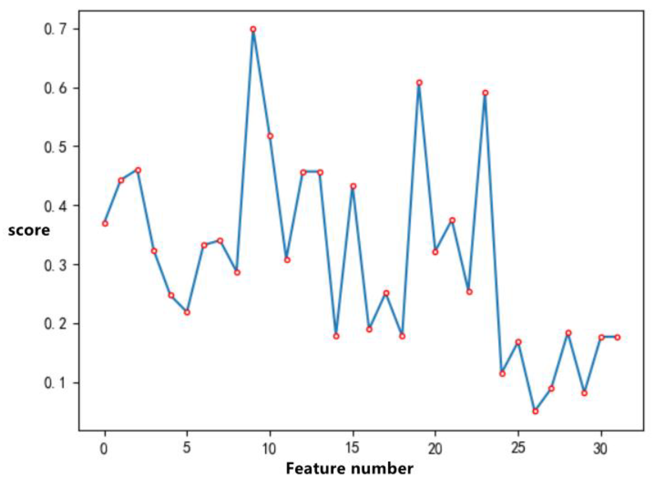
In this experiment, the 32 extracted features were firstly analyzed using the sensitivity measurement standard, and the features that had less impact on subsequent processing were deleted by cross-validation. The remaining features form a new feature set. The characteristic sensitivity analysis diagram is drawn through the sensitivity analysis, as shown in Figure 3.

The new feature set is then used to carry out the SVM-RFE model to continue the retrograde training, assign the feature importance and sort it, delete the least important feature, in turn, analyze, and finally find the optimal set. According to the screening results, data analysis is performed on the five categories of water, high, building, low, and road, and compared with those before the screening. Analysis of the results before and after screening is shown in

Table 1. Category analysis before screening.

Class	Kappa	Precision	Recall	F1-Score
water	0.68	0.93	0.90	0.91
high	0.68	0.88	0.93	0.90
building	0.68	0.60	0.65	0.62
low	0.68	0.86	0.74	0.80
road	0.68	0.50	0.51	0.50

and

Table 2. Category analysis after screening.

Class	Kappa	Precision	Recall	F1-Score
water	0.74	0.91	0.92	0.92
high	0.74	0.92	0.91	0.91
building	0.74	0.65	0.66	0.65
low	0.74	0.86	0.88	0.87
road	0.74	0.61	0.59	0.60

.

It can be seen that compared with 32 feature sets, the accuracy of optimal feature collection, recall index and F1 parameters have been greatly improved. Among them, the accuracy of water and high has reached more than 0.9.

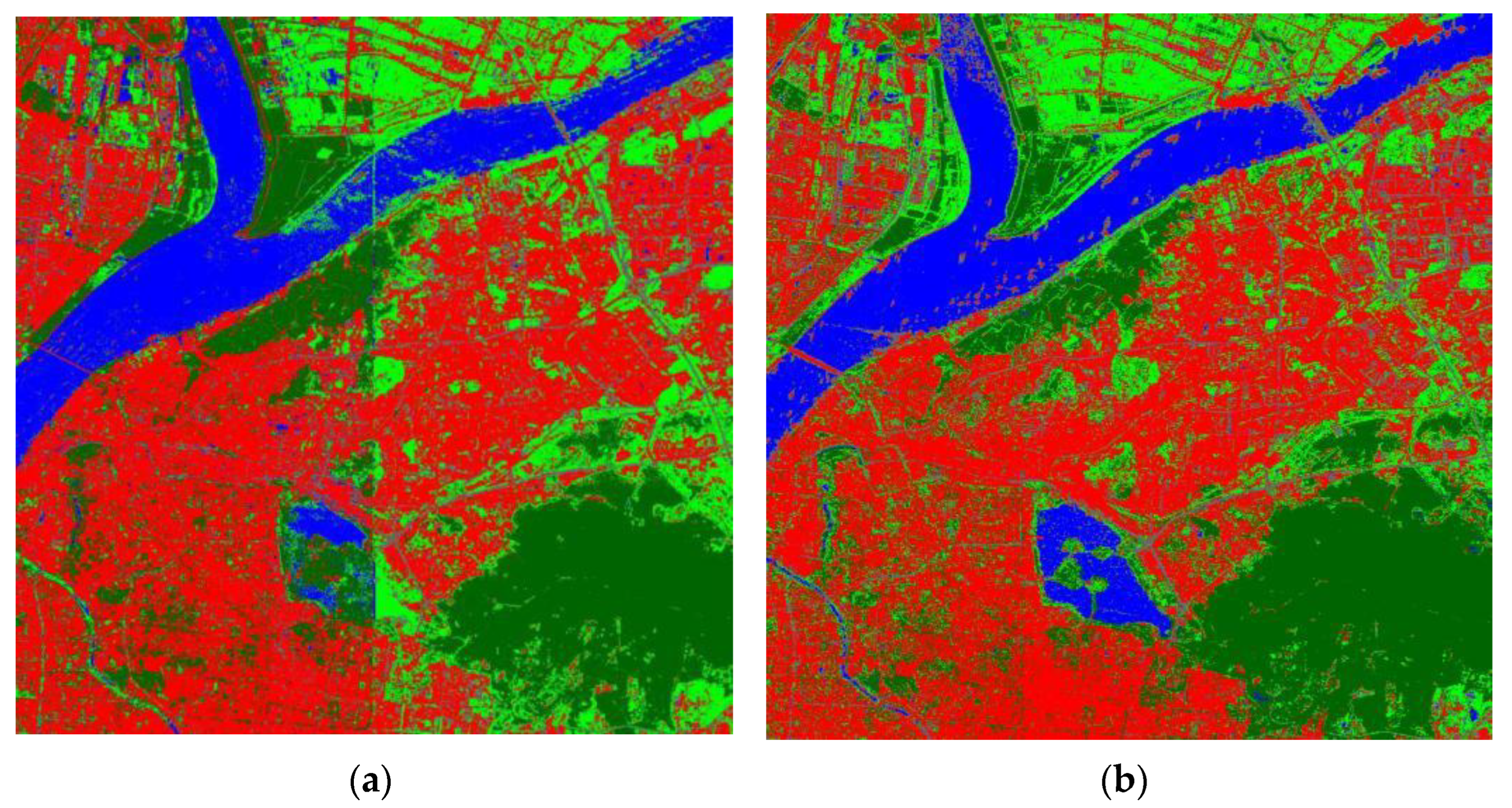
Next, we performed classification experiments and compared the filtered feature set with the unfiltered feature set. The comparison of classification effects before and after feature filtering is shown in Figure 4.

After the trained classifier classifies the entire image, it can be seen that the classification accuracy after screening has been significantly improved, especially the classification effect of the water category has improved significantly, and the image smoothness has also been significantly improved. The above results show that features’ screening and sorting results are reliable.

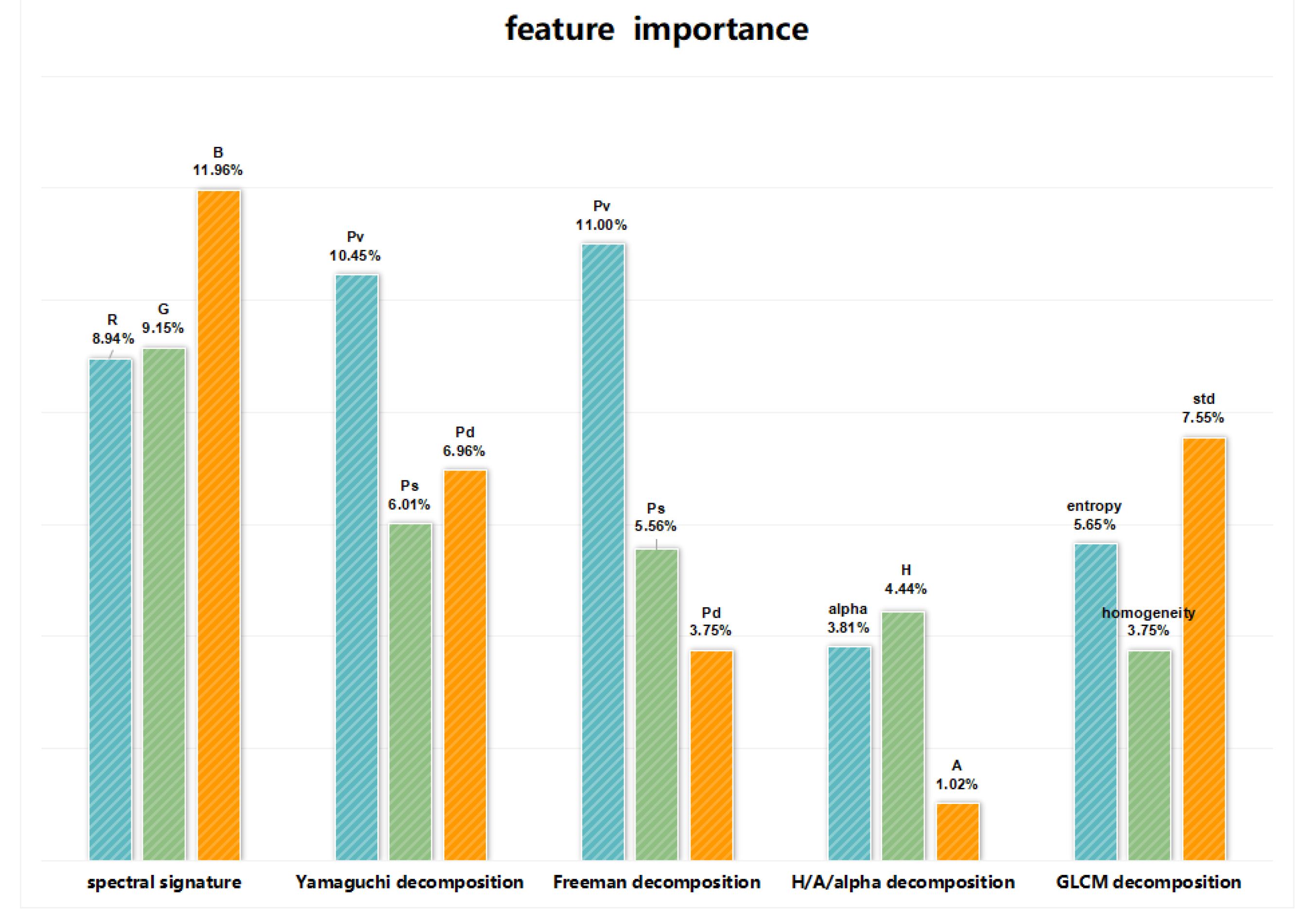
Finally, the importance of all features is sorted out according to the continuous iteration, and the feature importance ratio shown in Figure 5 is obtained. The importance of all features of polarimetric SAR images accounts for about 70%, and the importance of all features of optical images accounts for about 30%. Therefore, the optimal values of the weighting coefficients ${\lambda }_{optical}$ and ${\lambda }_{SAR}$ of the binary potential function of the polarimetric SAR image and the optical image are 0.7 and 0.3, which are brought into Formula (9) for the next experiment.

4.2. Comparison of Results of Input Single-Polarization and Full-Polarization SAR Images in the CRF Model

In order to verify that the dual-channel multi-scale convolutional CRF model proposed in this paper inputs a full-polarization SAR image or a single-polarization SAR image, and the segmentation effect of the front-end network is greatly improved, this section uses the full-polarization SAR image and the single-polarization SAR image. Polarimetric SAR images are segmented on a dual-channel multi-scale convolutional CRF, respectively, and the segmentation results are compared.

This paper quantitatively measures network performance using pixel intersection-over-union (IoU), mean intersection-over-union (mIoU), and global accuracy (GA), including:

$$\mathrm{GA}=\frac{{\displaystyle \sum _{i=1}^k{n}_{ii}}}{{\displaystyle \sum _{i=1}^k{t}_i}}$$

(42)

$$Io{U}_{cls}=\frac{n_{ii}}{t_i-n_{ii}+{\displaystyle \sum _j^k{n}_{ji}}}$$

(43)

$$mIoU=\frac{1}{k}{\displaystyle \sum _{i=1}^k\frac{n_{ii}}{t_i-n_{ii}+{\displaystyle \sum _{j=1}^k{n}_{ji}}}}$$

(44)

$t_i$ represents the total number of pixel $i$. $k$ represents the number of categories of pixels. $n_{ij}$ represents the number of pixel categories $i$ is predicted to be in the category $j$. GA is a good way to show that the network training precision, $Io{U}_{cls}$, is also the appropriate punishment for the classification of network errors, and the two complement each other, while $Io{U}_{cls}$ only represents the network’s prediction accuracy of a single pixel. In order to obtain a general evaluation of the overall evaluation results, the average of the $mIoU$ is compared to the overall semantic segmentation accuracy of the network for all pixels.

Here, the full-polarization SAR images of Nanjing and surrounding areas are randomly flipped and mirrored and then input into the CRF model proposed in this paper for processing. The results obtained are shown in

Table 3. Comparison of segmentation results of using single-polarization and full-polarization SAR images.

Method	$\mathit{A}\mathit{c}\mathit{c}\mathit{u}\mathit{r}\mathit{a}\mathit{c}\mathit{y}$	$\mathit{I}\mathit{o}{\mathit{U}}_{\mathit{c}\mathit{l}\mathit{s}0}$	$\mathit{I}\mathit{o}{\mathit{U}}_{\mathit{c}\mathit{l}\mathit{s}1}$	$\mathit{I}\mathit{o}{\mathit{U}}_{\mathit{c}\mathit{l}\mathit{s}2}$	$\mathit{I}\mathit{o}{\mathit{U}}_{\mathit{c}\mathit{l}\mathit{s}3}$	$\mathit{I}\mathit{o}{\mathit{U}}_{\mathit{c}\mathit{l}\mathit{s}4}$	$\mathit{m}\mathit{I}\mathit{o}{\mathit{U}}_{\mathit{c}\mathit{l}\mathit{s}}$	Time [ms]
FullCRF with single-polarization	85.13%	96.24%	88.13%	96.55%	92.22%	36.15%	81.92%	273
ConvCRF with single-polarization	89.56%	96.44%	89.60%	95.01%	93.08%	55.98%	85.37%	14
Improved CRF with single-polarization	90.25%	96.97%	89.69%	95.51%	93.48%	57.16%	86.56%	9
Improved CRF with full-polarization	90.27%	97.02%	90.11%	95.58%	94.46%	57.27%	87.05%	12

.

In Table 3, the subscripts $cls0,cls1,cls2,cls3,cls4$ represent five different pixel category labels: {0: background (black)}, {1: river (red)}, {2: plain (green)}, {3: building (yellow)}, {4: road (blue)}, $mIo{U}_{cls}$ represents the average pixel intersection ratio result of five pixel categories. It can be seen from Table 3 that the performance of the network has been improved to a certain extent when the full-polarization SAR image is used as the input image of the CRF, the model accuracy, $Io{U}_{cls0}$, $Io{U}_{cls1}$ and $Io{U}_{cls2}$ have been improved to a certain extent, and the $Io{U}_{cls3}$ of Improved CRF has been improved by 1%. In addition, it can be seen from Table 3 that the segmentation effect of the Improved CRF is much better than that of other models when single-polarization SAR images are used. After the input of fully polarized SAR image, the segmentation effect is much better than other models.

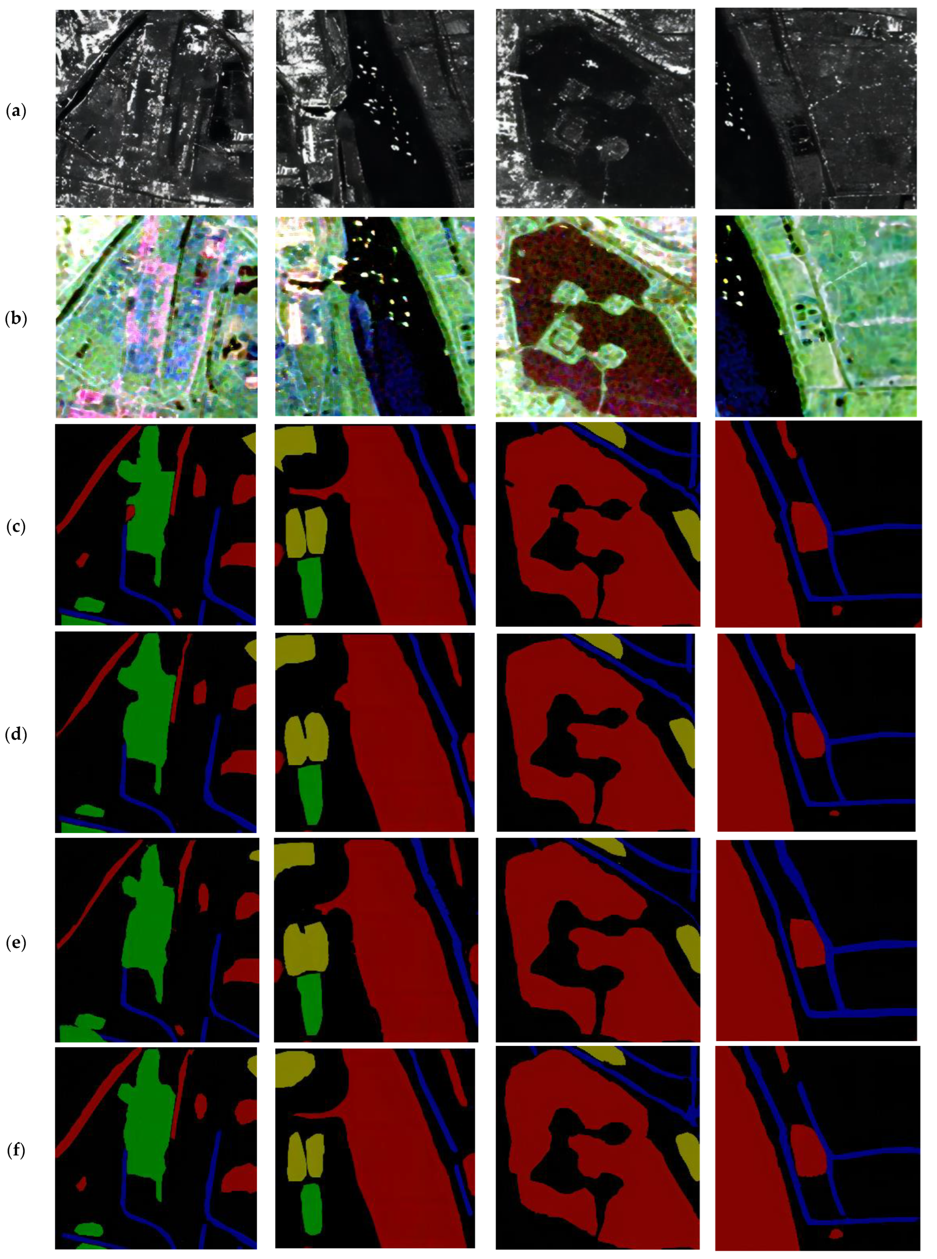
Figure 6 shows the results of using the full-polarization SAR image input model. The figure, from top to bottom, is the single-polarization SAR image, the full-polarization SAR image, the label image, the output of the FullCRF with single-polarization SAR image, the output of the ConvCRF with single-polarization SAR image, the output of the Improved CRF with single-polarization SAR image, and the output of the Improved CRF with full-polarization SAR image. The part enclosed in the red box represent the sections with the best segmentation. It can be seen from Figure 6 that after the full polarization, the SAR image is input into the model, the image segmentation is more accurate, the boundary is clearer, and some small areas can be divided. After comparison, it can be found that the full-polarization SAR image contains more features, which can clarify the spatial relationship between the target and the neighborhood, and improve the classification accuracy. At the same time, when full-polarization SAR images are input into different CRF models, it can be found that the dual-channel multi-scale fully connected convolutional CRF model proposed in this paper can achieve a better semantic segmentation effect in full-polarization SAR images. It is obvious from the part enclosed by the box in the picture that the method proposed in this paper can be segmented more carefully at the boundaries of different regions. Both FullCRF and ConvCRF models have varying degrees of confusion in the details.

4.3. Results of Two-Channel Multi-Scale Convolutional CRF on Synthetic Data

The model is first evaluated on synthetic data to demonstrate the capabilities of a two-channel multi-scale convolutional CRF. At this time, by adding noise to the label image as the basis of the unary potential function and then processing the synthetic data by the model, the output results of the three models are finally compared with the original label image.

Here, the label map is first downsampled by a factor of eight, and then the downsampled image is randomly flipped and mirrored. The result is upsampled to restore the original resolution, and finally, the data are input into the three models. The treatment was carried out, and the results obtained are shown in

Table 4. Results of three fully connected CRFs on synthetic data.

Method	$\mathit{A}\mathit{c}\mathit{c}\mathit{u}\mathit{r}\mathit{a}\mathit{c}\mathit{y}$	$\mathit{I}\mathit{o}{\mathit{U}}_{\mathit{c}\mathit{l}\mathit{s}0}$	$\mathit{I}\mathit{o}{\mathit{U}}_{\mathit{c}\mathit{l}\mathit{s}1}$	$\mathit{I}\mathit{o}{\mathit{U}}_{\mathit{c}\mathit{l}\mathit{s}2}$	$\mathit{I}\mathit{o}{\mathit{U}}_{\mathit{c}\mathit{l}\mathit{s}3}$	$\mathit{I}\mathit{o}{\mathit{U}}_{\mathit{c}\mathit{l}\mathit{s}4}$	$\mathit{m}\mathit{I}\mathit{o}{\mathit{U}}_{\mathit{c}\mathit{l}\mathit{s}}$	Time [ms]
Unary	80.51%	97.79%	90.65%	98.45%	95.86%	15.43%	79.64%	66
FullCRF	85.35%	97.51%	90.22%	97.79%	94.34%	36.15%	83.20%	273
ConvCRF	90.07%	97.02%	90.11%	95.58%	93.48%	56.32%	86.50%	15
Improved CRF	91.91%	98.24%	94.39%	98.30%	95.64%	57.53%	88.82%	15

. Unary represents the result of synthetic data, FullCRF and ConvCRF represent the fully connected conditional random field and convolutional fully connected conditional random field using tetrahedral lattice approximation message passing, respectively.

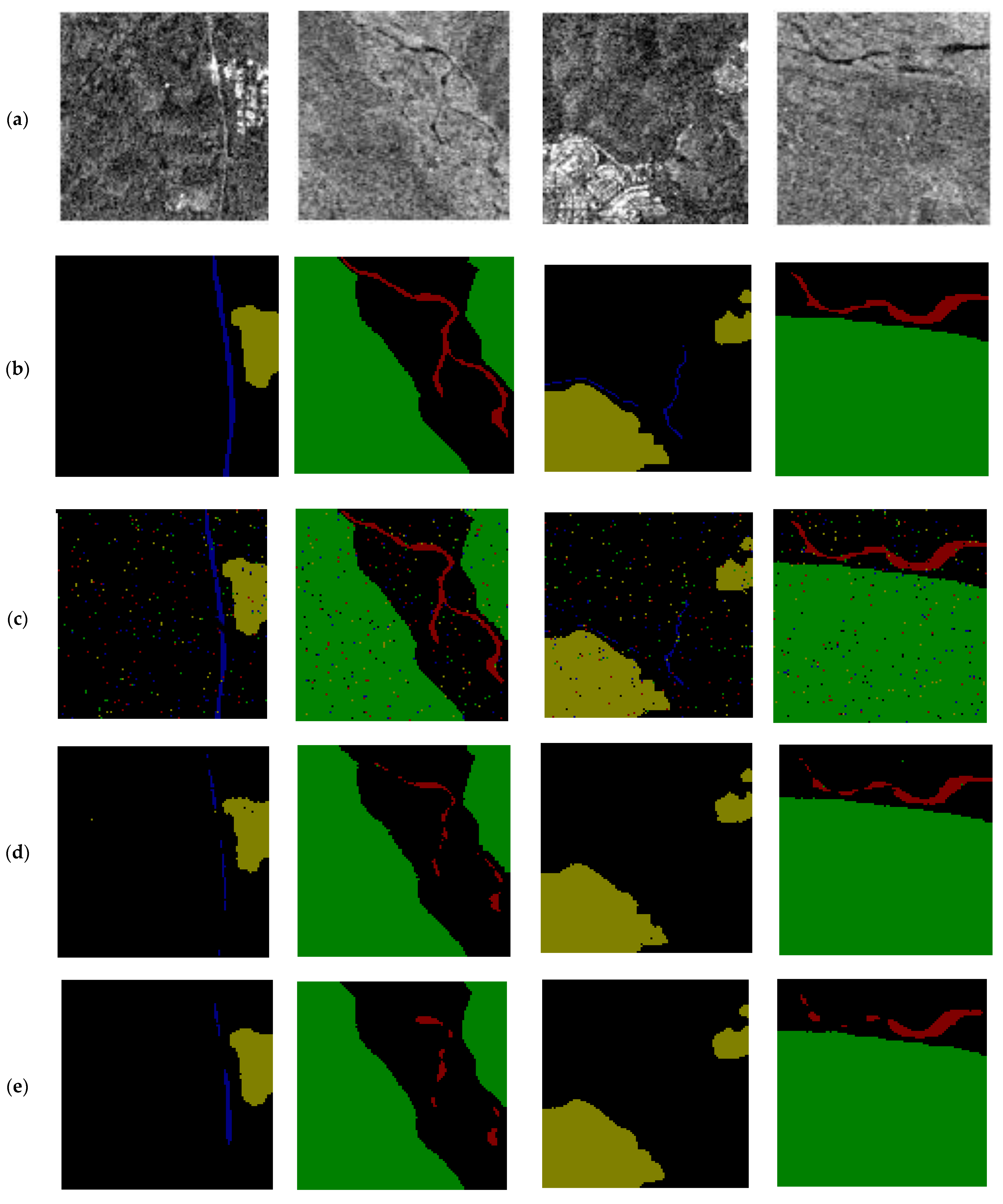
As shown in Table 4, the convolutional conditional random field ConvCRF is significantly better than the original conditional random field, and there is a significant improvement in both accuracy and time consumption. This is because precise message passing is used in ConvCRF. Instead of the tetrahedral lattice approximation in FullCRF, the improved two-channel multi-size convolutional conditional random field has higher accuracy. Feature information, such as location, enables the entire model to utilize more spatial semantic information between pixels; simultaneously, because of the use of multi-size input, the model can obtain more feature information by modeling images of different resolutions. The results of several models are shown in Figure 7, from top to bottom, the polarimetric SAR image, label map, synthetic data, FullCRF output, ConvCRF output, and the output of the proposed method. The part enclosed in the red box represent the sections with the best segmentation. It is obvious from the part enclosed by the box in the picture that the method proposed in this paper is closer to the actual label image for the synthetic data processing result, which further proves the effectiveness of the method proposed in this paper.

4.4. Results of Two-Channel Multi-Scale Convolutional CRF on Polarimetric SAR Images

In this section, the model is used to further post-process the semantic segmentation of polarimetric SAR images. The unary potential function is constructed by using the predicted probability values of different class labels output by the last $soft\max$ layer of the deep convolutional neural network, and the binary potential function is still established based on the optical and polarimetric SAR images of the two-channel input; the model parameters remain unchanged; and the average value is also used. The approximate field inference is iteratively calculated five times, and finally, the semantic segmentation post-processing results of the three models are obtained, as shown in

Table 5. Post-processing results of three models for semantic segmentation of polarimetric SAR images.

Method	$\mathit{A}\mathit{c}\mathit{c}\mathit{u}\mathit{r}\mathit{a}\mathit{c}\mathit{y}$	$\mathit{I}\mathit{o}{\mathit{U}}_{\mathit{c}\mathit{l}\mathit{s}0}$	$\mathit{I}\mathit{o}{\mathit{U}}_{\mathit{c}\mathit{l}\mathit{s}1}$	$\mathit{I}\mathit{o}{\mathit{U}}_{\mathit{c}\mathit{l}\mathit{s}2}$	$\mathit{I}\mathit{o}{\mathit{U}}_{\mathit{c}\mathit{l}\mathit{s}3}$	$\mathit{I}\mathit{o}{\mathit{U}}_{\mathit{c}\mathit{l}\mathit{s}4}$	$\mathit{m}\mathit{I}\mathit{o}{\mathit{U}}_{\mathit{c}\mathit{l}\mathit{s}}$	Time [ms]
Deeplabv3+	90.57%	97.20%	96.63%	95.92%	88.80%	46.84%	85.08%	15
ConvCRF	87.34%	96.91%	89.26%	95.55%	93.45%	47.99%	84.63%	273
FullCRF	89.58%	96.90%	89.84%	95.52%	93.01%	54.18%	85.88%	13
Improved CRF	90.25%	96.97%	89.69%	95.51%	93.48%	57.16%	86.56%	9

.

Among them, Deeplabv3+ represents the semantic segmentation result of polarimetric SAR image output by the previous deep convolutional neural network, which is used here as the primary input of the unary potential function of the three fully connected conditional random fields. It can be seen from Table 5 that the improvements of the three models to the Deeplabv3+ network are mainly on the latter two labels, namely buildings and roads. In comparison, the method proposed in this paper has the most significant improvement. Compared with Deeplabv3+, $Io{U}_{cls3}$ Table 1 is improved by 4.68%, The $Io{U}_{cls4}$ is increased by 10.32%, and the final $mIoU$ of all pixel categories increases by 1.48% compared with the previous Deeplabv3+ network output. At the same time, this paper uses multi-size input, and the final comprehensive average time is reduced by 4 ms compared to direct input of a single size polarimetric SAR image. However, the improvement effect for the categories mentioned above is not apparent. The results of several models are shown in Figure 8. From top to bottom in the figure are the polarimetric SAR image, the label map, the Deelabv3+ network output, the FullCRF output, the ConvCRF output, and the output of the proposed method in this paper. The part enclosed in the red box represent the sections with the best segmentation. As can be seen from Figure 8, the semantic segmentation results obtained by Deeplabv3+ are output by three full-connection conditional random field models. It is the easier to distinguish between different pixel categories; that is, the boundary of each pixel category is smoother. By comparing Figure 8, the last three lines show that the method proposed in this paper achieves the best results.

In recent years, there has been much research on semantic segmentation using conditional random fields. Excellent improvements to semantic segmentation networks also emerge, such as the improved PSPNet and ConvCRF model proposed by WANG Junqiang [16]. Compared with these methods, the method proposed in this paper has a more novel technology in the aspect of feature information expansion, which can make full use of the data feature information. The method proposed in this paper adds a CRF post-processing model on the basis of Deeplabv3+ Network [17]. The optical image and SAR image are input into the model at the same time, and the input ratio is optimized. The original single-polarization SAR image is changed to a full-polarization SAR image. Through the above three experiments, it is proven that the model proposed in this paper has the best effect compared with the previous model.

5. Conclusions

In this paper, a two-channel multi-scale fully connected convolutional conditional random field method is proposed for the semantic segmentation of polarimetric SAR images. Firstly, this paper inputs the full-polarization SAR image and the single-polarization SAR image into the CRF model for comparative experiments and confirms that the full-polarization SAR image input to the CRF model can improve the segmentation effect. The feature information in polarimetric SAR images increases and the number of features that the model can refer to for polarimetric SAR image segmentation is further expanded. Secondly, based on the convolutional CRF, a dual-channel fusion of the feature information, such as the spectrum and position of the pixels included in the optical image and multi-scale input, is proposed, which improves the recognition accuracy of roads and buildings to a certain extent, and improves the original network. Finally, using the SVM-RFE algorithm based on sensitivity analysis, the characteristics of polarimetric SAR images and optical images are screened and sorted, and the polarimetric SAR images and optical images are determined according to the results and input to the network at the same time. Using such a contribution degree as the weight in the CRF pairwise potential function clarifies the spatial relationship between the target and the neighborhood and improves classification accuracy. Experiments show that this method can improve the recognition accuracy of the algorithm and effectively reduce the model inference and training time in the segmentation task of polarimetric SAR images. The model achieves better performance indicators, compared with Deeplabv3+, $Io{U}_{cls3}$ is improved by 4.68%, $Io{U}_{cls4}$ is increased by 10.32%, and the final $mIoU$ of all pixel categories increases by 1.48%, and average time is reduced by 4 ms compared with the previous Deeplabv3+ network output. Although the proposed model achieves a good performance in SAR image semantic segmentation, it still needs to be improved. We directly fuse the color and position features of the SAR image and optical image corresponding to the pixel target through simple convolution operation to obtain the feature vector, which will lose some important semantic information of pixels. In the future, we will develop more effective feature fusion methods to further improve the post-processing effect of the model.

References

1. Li, S.Z. Markov Random Field Modeling in Image Analysis; Springer: London, UK, 2009. [Google Scholar]
2. Duan, Y.; Liu, F.; Jiao, L.; Zhao, P.; Zhang, L. SAR Image segmentation based on convolutional-wavelet neural network and markov random field. Pattern Recognit. 2017, 64, 255–267. [Google Scholar] [CrossRef]
3. Bouhlel, N.; Méric, S. Unsupervised Segmentation of Multilook Polarimetric Synthetic Aperture Radar Images. IEEE Trans. Geosci. Remote Sens. 2019, 57, 6104–6118. [Google Scholar] [CrossRef]
4. Wang, F.; Wu, Y.; Li, M.; Zhang, P.; Zhang, Q. Adaptive Hybrid Conditional Random Field Model for SAR Image Segmentation. IEEE Trans. Geosci. Remote Sens. 2017, 55, 537–550. [Google Scholar] [CrossRef]
5. Ladický, L.; Russell, C.; Kohli, P.; Torr, P.H.S. Associative hierarchical CRFs for object class image segmentation. In Proceedings of the 2009 IEEE 12th International Conference on Computer Vision Workshops, Kyoto, Japan, 27 September–4 October 2009; pp. 739–746. [Google Scholar]
6. Zhong, Y.; Zhao, J.; Zhang, L. A hybrid object-oriented conditional random field classification framework for high spatial resolution remote sensing imagery. IEEE Trans. Geosci. Remote Sens. 2014, 52, 7023–7037. [Google Scholar] [CrossRef]
7. Zhong, P.; Wang, R. Multiple-spectral-band CRFs for denoising junk bands of hyperspectral imagery. IEEE Trans. Geosci. Remote Sens. 2013, 51, 2260–2275. [Google Scholar] [CrossRef]
8. Heili, A.; López-Méndez, A.; Odobez, J.-M. Exploiting long-term connectivity and visual motion in CRF-based multi-person tracking. IEEE Trans. Image Process. 2014, 23, 3040–3056. [Google Scholar] [CrossRef] [PubMed] [Green Version]
9. Krähenbühl, P.; Koltun, V. Efficient inference in fully connected CRFs with gaussian edge potentials. Adv. Neural Inf. Process. Syst. 2011, 24, 109–117. [Google Scholar]
10. Zheng, S.; Jayasumana, S.; Romera-Paredes, B.; Vineet, V.; Su, Z.; Du, D.; Huang, C.; Torr, P.H.S. Conditional Random Fields as Recurrent Neural Networks. In Proceedings of the 2015 IEEE International Conference on Computer Vision (ICCV), Santiago, Chile, 7–13 December 2015. [Google Scholar]
11. Teichmann, M.; Cipolla, R. Convolutional CRFs for Semantic Segmentation. arXiv 2018, arXiv:1805.04777. [Google Scholar]
12. Qiu, Y.; Cai, J.; Qin, X.; Zhang, J. Inferring Skin Lesion Segmentation with Fully Connected CRFs based on Multiple Deep Convolutional Neural Networks. IEEE Access 2020, 8, 144246–144258. [Google Scholar] [CrossRef]
13. Jun, C.; Peijun, D.; Kun, T. A supervised classification algorithm for fully polarized synthetic aperture radar based on Pauli decomposition and support vector machine. Sci. Technol. Eng. 2014, 17, 6. [Google Scholar]
14. Hang, L. Statistical Learning Methods; Tsinghua University Press: Beijing, China, 2012. [Google Scholar]
15. Yamaguchi, Y.; Yajima, Y.; Yamada, H. A four component decomposition of POLSAR images based on the coherence matrix. IEEE Trans. Geosci. Remote Sens. Lett. 2006, 3, 292–296. [Google Scholar] [CrossRef]
16. Junqiang, W.; Feng, W.; Minggui, T.; Cheng, Z. Remote Sensing Image Segmentation based on improved PSPNet and ConvCRF. Geogr. Inf. World 2021, 28, 8. [Google Scholar]
17. Kong, Y.; Liu, Y.; Yan, B.; Leung, H.; Peng, X. A Novel Deeplabv3+ Network for SAR Imagery Semantic Segmentation Based on the Potential Energy Loss Function of Gibbs Distribution. Remote Sens. 2021, 13, 454. [Google Scholar] [CrossRef]
Figure 1. Schematic diagram of the model structure.
Remotesensing 14 01502 g001
Figure 2. Flow chart of SVM-RFE algorithm based on sensitivity analysis.
Remotesensing 14 01502 g002
Figure 3. Sensitivity analysis results.
Remotesensing 14 01502 g003
Figure 4. Classification effect diagram: (a) the unfiltered feature set; (b) the filtered feature set.
Remotesensing 14 01502 g004
Figure 5. Sensitivity analysis results.
Remotesensing 14 01502 g005
Figure 6. Model prediction results: (a) single-polarization SAR image, (b) full-polarization SAR image, (c) label image, (d) output of single-polarization, (e) FullCRF, (f) ConvCRF, (g) output of Improved CRF.
Remotesensing 14 01502 g006aRemotesensing 14 01502 g006b
Figure 7. Model prediction results: (a) polarimetric SAR image, (b) label image, (c) synthetic data (Unary), (d) FullCRF, (e) ConvCRF, (f) the method of this paper.
Remotesensing 14 01502 g007aRemotesensing 14 01502 g007b
Figure 8. Model prediction results:(a) polarimetric SAR image, (b) label image, (c) Deelabv3+, (d) FullCRF, (e) ConvCRF, (f) the method of this paper.
Remotesensing 14 01502 g008aRemotesensing 14 01502 g008b