Spatial Transferability of Random Forest Models for Crop Type Classification Using Sentinel-1 and Sentinel-2

Abstract

Large-scale crop type mapping often requires prediction beyond the environmental settings of the training sites. Shifts in crop phenology, field characteristics, or ecological site conditions in the previously unseen area, may reduce the classification performance of machine learning classifiers that often overfit to the training sites. This study aims to assess the spatial transferability of Random Forest models for crop type classification across Germany. The effects of different input datasets, i.e., only optical, only Synthetic Aperture Radar (SAR), and optical-SAR data combination, and the impact of spatial feature selection were systematically tested to identify the optimal approach that shows the highest accuracy in the transfer region. The spatial feature selection, a feature selection approach combined with spatial cross-validation, should remove features that carry site-specific information in the training data, which in turn can reduce the accuracy of the classification model in previously unseen areas. Seven study sites distributed over Germany were analyzed using reference data for the major 11 crops grown in the year 2018. Sentinel-1 and Sentinel-2 data from October 2017 to October 2018 were used as input. The accuracy estimation was performed using the spatially independent sample sets. The results of the optical-SAR combination outperformed those of single sensors in the training sites (maximum F1-score–0.85), and likewise in the areas not covered by training data (maximum F1-score–0.79). Random forest models based on only SAR features showed the lowest accuracy losses when transferred to unseen regions (average F1_loss–0.04). In contrast to using the entire feature set, spatial feature selection substantially reduces the number of input features while preserving good predictive performance on unseen sites. Altogether, applying spatial feature selection to a combination of optical-SAR features or using SAR-only features is beneficial for large-scale crop type classification where training data is not evenly distributed over the complete study region.

1. Introduction

Supervised machine learning methods are widely used for large-scale crop type classification [1,2,3]. Due to the limited availability of field data (e.g., because of location inaccessibility or reference data collection costs), large-scale crop type mapping often implies model predictions in geographical spaces far beyond the training locations. Due to the presence of spatial autocorrelation in the geo-referenced datasets, the predictor variables in reference systems (i.e., the training sites) might significantly differ from those in transfer systems (i.e., unseen by model transfer sites). Spatially transferring the model outside the ‘known’ to a model environment could substantially reduce its performance. In the context of crop type mapping, the good spatial transferability of a machine learning classifier indicates its ability to predict crop classes in unseen environments with minimal accuracy losses compared with classification accuracies achieved in training areas.

In recent years, the spatial transferability of machine learning models has been rigorously studied in various geo-spatial application fields (e.g., land cover classification [4], species distribution modelling [5]). Many crop type classification studies have illustrated the successful use of transfer learning and domain adaptation techniques [6,7,8]. For example, Bazzi et al. (2020) [9] applied ‘distil and refine’ approach, where the Convolutional Neural Network (CNN) trained with large reference system samples is first distilled into a smaller ‘student’ model and then refined using the limited target system samples for mapping irrigated areas. Lucas et al. (2021) [10] presented a semi-supervised domain adaptation technique with a novel regularisation method for CNN for mapping a wide variety of crops with the limited number of samples available in the target system. Gilcher and Udelhoven (2021) [11] compared the spatial and temporal transferability of pixel-based and convolution-based classifiers for binary maize and non-maize classification using Synthetic Aperture Radar (SAR) data. Hao et al. (2020) [12] researched how the length of time-series of Normalized Difference Vegetation Index (NDVI) features affects the predictive performance of Random Forest models in target systems. Most of such studies were investigating the classifier adaptation techniques to the target domain using semi-supervised or unsupervised learning. In comparison, much less research is available on the influence of input remote-sensing datasets on the classifier’s performance in the target systems as performed by, e.g., Hao et al. (2020) [12].

Besides the lack of representative samples, overfitting of a classification model to reference samples is a major reason for poor spatial transferability and hence poor generality. Spatial overfitting can occur when machine learning algorithms such as Random Forest are optimized, e.g., for the training data acquired from certain localities [13]. Recent studies have illustrated that a reduction in spatial overfitting, i.e., fitting the model to samples of one location exclusively, is possible by performing spatial cross-validation (CV) based feature selection [14,15], also known as spatial feature selection. Spatial feature selection allows detecting and removing problematic predictor variables that carry information about specific training sites but negatively affect the accuracy of predictions in a new geo-location [16]. Such approaches to feature selection fall into the ‘invariant feature selection’ category of domain adaptation techniques [17]. While spatial feature selection showed improvements in model transferability in other research fields [14], the effect of spatial feature selection on improving the spatial transferability of crop type mapping has not yet been tested.

The type of remote-sensing datasets used for crop type classification has a substantial effect on crop type accuracies [18]. Many studies underpin higher classification accuracy based on optical-SAR combinations than single sensor datasets [19,20,21]. Joint use of sensors provides complementary information, such as plant pigment information and canopy structure, and allows improved discrimination of crop types [22]. However, to the best of our knowledge, it is unknown if Random Forest models for crop type mapping based on the combination of optical-SAR data show superior results when spatially transferred to the previously unseen environment compared with single-sensor models. Moreover, no comparative studies were found investigating the spatial transferability of models based on only optical and only-SAR datasets. Operational SAR sensors such as Sentinel-1 observe the Earth’s surface through clouds at regular intervals over large spaces. Whereas acquisitions from optical data are less regular due to the clouds, which in turn affect the generation of regular time series. It can be hypothesised that SAR-based models with more regular data acquisitions would perform better concerning spatial transferability to distant geographical spaces than optical datasets. This hypothesis is relevant to the areas where the persistent presence of clouds could substantially affect the quality of optical features.

Against this background, this study aims to quantify, reduce, and assess the accuracy losses introduced through the spatial transfer of Random Forest models for crop type mapping in the example of the diverse agricultural landscapes of Germany. First, we test the performance of single SAR or optical data in comparison to a combination of both when predicting crop type classes in a target system, i.e., the transfer region. Second, we attempt to improve the spatial transferability of the widely used machine learning classifier Random Forest using spatial feature selection with a modified feature selection approach—three-step group-wise forward feature selection. Moreover, we analyse auxiliary information such as surface elevation, parcel sizes, soil quality rating, and phenological observation data to understand their possible influences on spatial transferability.

2. Study Sites and Data

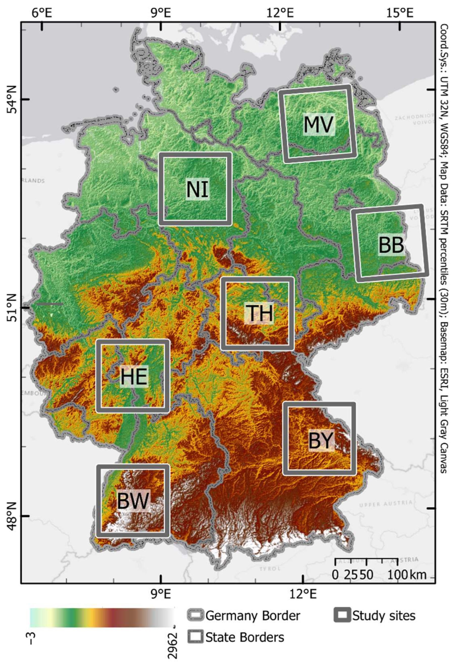
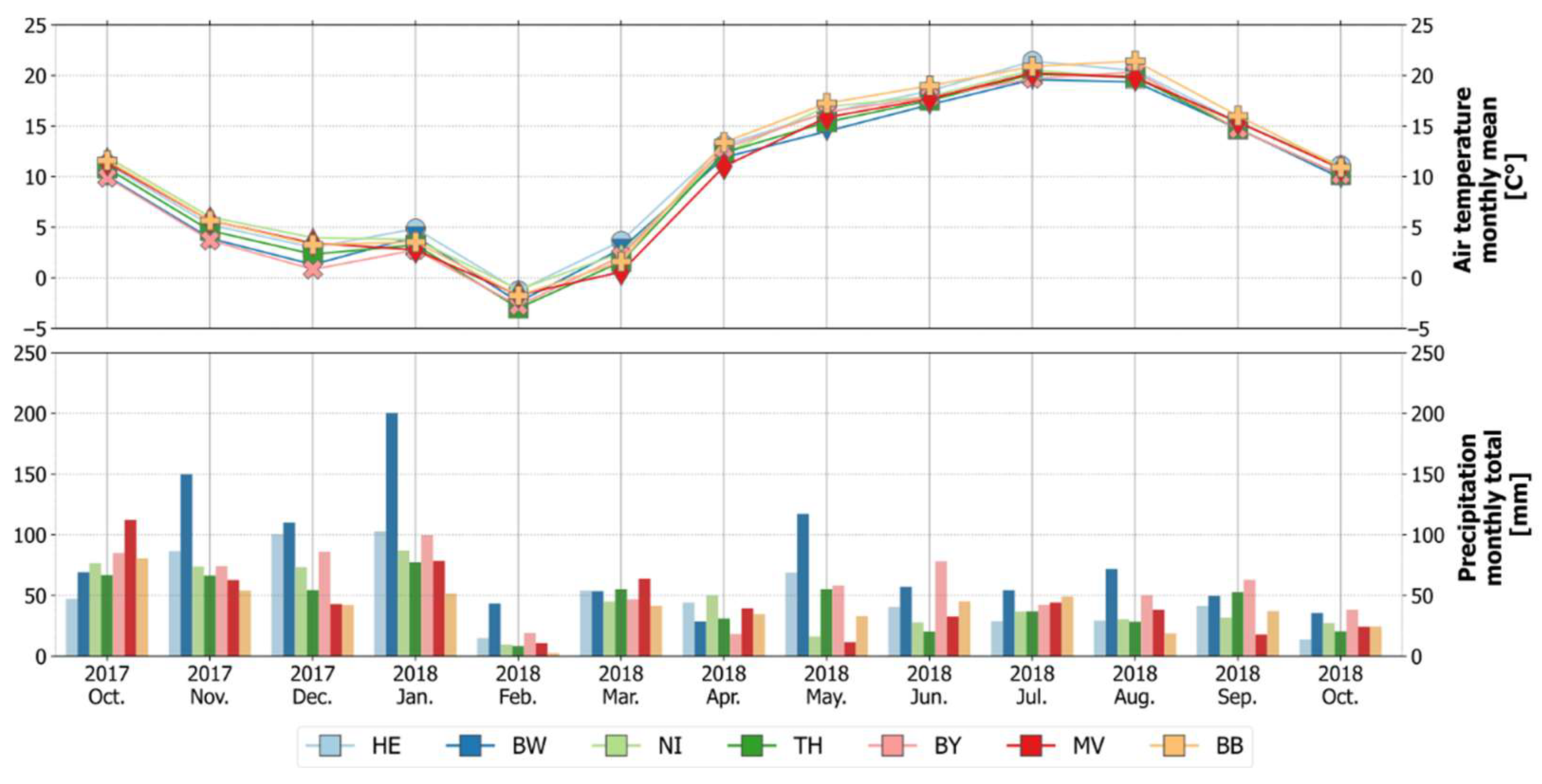
2.1. Study Sites

Seven study sites across Germany in the shape of Sentinel-2 tiles (109.8 km × 109.8 km) were chosen based on the reference data availability, the reference data quantity, the distance between study sites, and their regional dissimilarities (Figure 1). The acronyms of the study sites correspond to the second part of the ISO 3166-2 codes of the German federal states where the study sites are mainly located. (Here, BW-Baden-Württemberg, BY–Bavaria, BB–Brandenburg, HE–Hesse, MV–Mecklenburg-Western Pomerania, NI-Lower Saxony, TH–Thuringia). Three sites are located in the Northern German Lowlands (MV, BB, NI), one site in the Central Uplands (TH), two sites in the South German Scarplands (BW, HE), and another one in the Alpine Foreland (BY). The elevation gradually increases from the German Lowlands in the north to the Alps in the country’s south. Furthermore, we will use the codes of the German federal states to refer to the specific study site.

According to the present Köeppen-Geiger climate classification [23], the western three tiles (NI, HE, and BW) are located in class Cfb, which is characterised by a temperate oceanic climate with warm summers and no dry season. A warm-summer continental climate defines the eastern four tiles (TH, BY, MV, and BB) with no dry seasons (class Dfb). During the summer months of 2018, the lowest and the highest monthly mean air temperatures were recorded in tiles BY and BB [24]. The precipitation pattern varied over the year in all tiles [25]. The outstanding peaks of the monthly total precipitation occurred in tile BW (Figure 2). In general, the year 2018 was recorded as the warmest and sunniest year in Germany since at least 1881 [26], with the longest heat periods in July and August. This led to substantial negative anomalies in remotely sensed vegetation activity on agricultural land [27] and substantial yield losses [28]. However, the spatial patterns of anomalies recorded in 2018 were different across the country. It was a good study case for the assessment of the spatial transferability of Random Forest models under varying environmental and climatic conditions at the country scale.

An agricultural season in Germany typically lasts from March to September for the majority of summer crops and from September to August of the following year for winter cereals. However, due to the differences in natural landscapes and abiotic factors across the country, regional variation of a few days or even weeks can occur in phenological crop growth stages [29].

2.2. Reference Data

The reference datasets were acquired from seven German federal states in the form of vector files containing agricultural parcels and crop types for the year 2018. These datasets rely on farmers’ crop declarations, which are part of a subsidy payment scheme within the European Union’s Common Agricultural Policy. Agricultural parcels were recorded in the context of the Integrated Administration and Control System (IACS) that is executed by national administrations (in Germany, at the federal state level) and uses the Land Parcel Identification System (LPIS) as a basis. We will refer to the reference datasets as ‘LPIS data.’

The declarations by farmers involve manual digitalization of parcel borders. In many cases, such datasets contain geometry overlaps. Parcels overlapping adjacent parcels by more than 500 m² and parcels with a parcel size of less than 0.1 ha were filtered out from the original dataset. These thresholds were selected empirically. The following spectrally inseparable classes were combined: Maize with flowering path, silo maize, and maize for biogas classes were merged into one ‘maize’ class; Starch potatoes and potatoes for food were merged into one ‘potatoes’ class; Temporal and permanent grasslands were merged into one ‘grasslands’ class. The ‘summer oat’ and ‘summer barley’ classes were merged into a general ‘summer cereals’ class. We selected all crop types that were present in all tiles and that had at least 20 parcels after filtering. The threshold of 20 polygons was set to limit the number of pixels sampled from one polygon. The resulting selection of crop types is shown in

Table 1. Number of parcels per crop type in each study site.

	HE	BW	NI	TH	BY	MV	BB	Sum
Grasslands	2563	124,977	55,511	25,233	95,925	22,766	19,615	346,590
Maize	9837	28,756	26,486	2762	37,947	4165	2383	112,336
Alfalfa	486	942	46	1007	532	103	516	3632
Potatoes	1390	561	6023	159	4551	360	206	13,250
Sunflowers	43	69	20	31	32	83	406	684
Winter wheat	29,547	22,397	13,149	10,495	32,742	5585	1259	115,174
Winter barley	8741	7959	6356	3418	17,511	2513	1065	47,563
Winter rape	9392	5433	5273	5327	5694	3746	860	35,725
Winter triticale	1721	4585	3293	839	5137	386	717	16,678
Winter rye	2497	846	9944	468	2069	1902	4195	21,921
Summer cereals	7017	11,399	10,065	3272	6001	1519	1176	40,449
Sum	73,234	207,924	136,166	53,011	208,141	43,128	32,398	754,002

.

2.3. Remote Sensing Data and Pre-Processing

Optical and SAR data sensed by the Multi-Spectral Instrument (MSI) onboard Sentinel-2 A/B and by the C-band SAR instrument onboard Sentinel-1 A/B were downloaded from the Copernicus Open Access Hub covering the time frame from 1 October 2017 to 31 October 2018. In total, 679 Sentinel-2 scenes and 3709 Sentinel-1 scenes (1898 scenes in ascending and 1811 in descending modes) were processed. Due to its all-weather sensing capabilities, SAR data provides more consistent and valid observations over time. Whereas the availability of valid optical data highly depends on the weather conditions of the sensed locations.

For the pre-processing of optical data, we used the MACCS-ATCOR Joint Algorithm (MAJA) version 3.3 [30]. From the available 12 Sentinel-2 bands, we selected three visible (B2, B3, B4), one near-infrared (B8), four red-edge (B5, B6, B7, and B8A), and two short-wave infrared (B11, B12) bands that were corrected for slope effects (so-called ‘FRE products’ from MAJA). The red-edge and short-wave infrared bands with a 20 m spatial resolution were resampled to 10 m using the nearest neighbour algorithm. Commonly used vegetation indices [21,31,32], namely, Normalized Difference Vegetation Index (NDVI), Normalized Difference Water Index (NDWI) and Normalized Difference Yellow Index (NDYI), were calculated from Sentinel-2 bands (Equations (1)–(3)).

$$\mathrm{NDVI}=\left(\mathrm{B}8-\mathrm{B}4\right)/\left(\mathrm{B}8+\mathrm{B}4\right)$$

(1)

$$\mathrm{NDWI}=\left(\mathrm{B}8-\mathrm{B}12\right)/\left(\mathrm{B}8+\mathrm{B}12\right)$$

(2)

$$\mathrm{NDYI}=\left(\mathrm{B}3-\mathrm{B}2\right)/\left(\mathrm{B}3-\mathrm{B}2\right)$$

(3)

We pre-processed Level-1 Ground Range Detected (GRD) and Interferometric Wide Swath (IWS) Sentinel-1 scenes using the S1TBX toolbox (v7.0.4) of the SNAP software. The following pre-processing steps were conducted: (1) applying orbit files; (2) removing GRD border noise; (3) thermal noise removal; (4) subset to the study site area; (5) radiometric calibration; (6) refined Lee speckle filtering (filter window size–5 × 5); (7) terrain flattening; (8) terrain correction; (9) conversion of data from digital numbers to decibels (dB). The output images were resampled with the nearest neighbour algorithm to 10 m spatial resolution using gdal’s gdalwarp utility.

We have used pre-processed co-polarized VV and cross-polarized VH bands in ascending and descending data acquisition modes. Additionally, we have calculated the VH/VV ratio for each data acquisition mode.

2.4. Auxiliary Data

To explore potential factors influencing the quality of the spatial transferability, we gathered auxiliary information such as parcel sizes, phenological observation records, surface elevation, and soil quality rating values for each sampled pixel. The parcel sizes were calculated based on the reference LPIS datasets. Surface elevation information was extracted from a digital elevation model of the Shuttle Radar Topography Mission SRTM [33]. We downloaded the Müncheberger soil quality rating layer from the product centre of the German Federal Institute for Geosciences and Natural Resources [34]. The Müncheberger soil quality rating, developed by the Leibniz-Centre for Agricultural Landscape Research (ZALF), comprises information on basic soil and soil hazard indicators [35]. For each sample pixel, we extracted scores that ranged from 0 to 100, where a higher score indicates better soil quality for cropping and grazing and higher crop yield potential. We further processed phenological observation records provided by German Weather Service (DWD) via the Climate Data Center [36] for maize, summer barley, summer oat, winter wheat, and winter rape crops for the season 2017–18.

3. Methodology

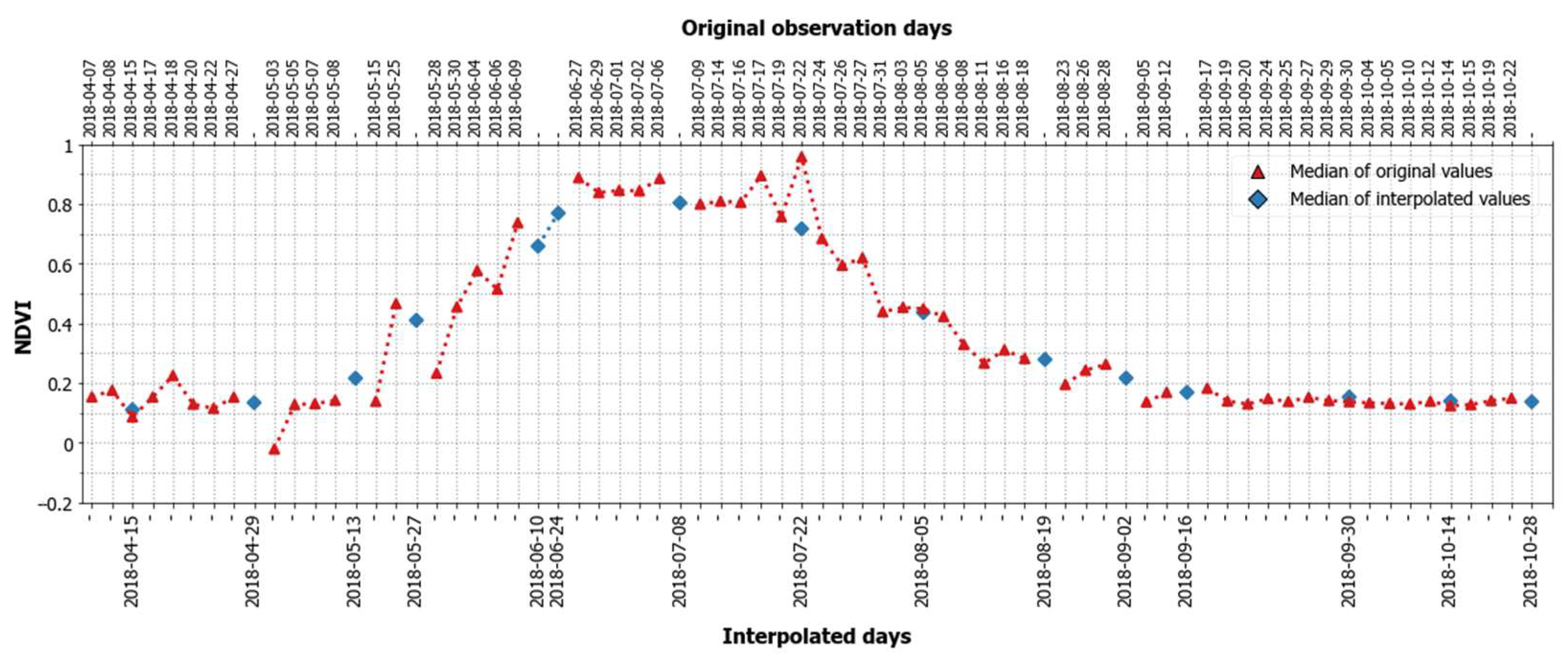
3.1. Generation of Dense Time Series Features

The remote-sensing data acquired for seven study sites are located in different orbit tracks, resulting in variation of data acquisition times across sites. In the case of optical data, clouds and cloud shadows reduce the consistency of the time-series. To generate evenly distributed dense time-series features for all study sites, we first generated bi-weekly datetime arrays from the 1 October 2017 to the 31 October 2018. The resulting 29 time-steps were used as the anchor dates to which we interpolated nearest (on time dimension) observation values from optical data (Figure 3). For SAR data, we selected images recorded seven days before and six days after the anchor date and calculated the median of these images at the pixel level. Generation of dense time-series features was performed for all optical and SAR variables described in Section 2.3.

3.2. Training and Testing Samples

The study was performed at the pixel-level to avoid the introduction of biases due to the segmentation quality across seven study sites [37]. For each of the seven study sites, we sampled 500 pixels per crop type using stratified random sampling. From the resulting sample set, 60 percent (300 pixels) was used as a training-set and 40 percent (200 pixels) as a test-set for the classification model. It was ensured that no overlaps occurred between training and test samples at the parcel level. To avoid the underrepresentation of samples from small parcels, we adjusted our sampling scheme to consider the parcel size information by distributing samples more evenly among parcels of different sizes. A negative buffer of 10 m (one Sentinel-2 pixel) was applied to exclude the border pixels from sampling. For each sample, we kept information about the size of the parcel from which it was sampled.

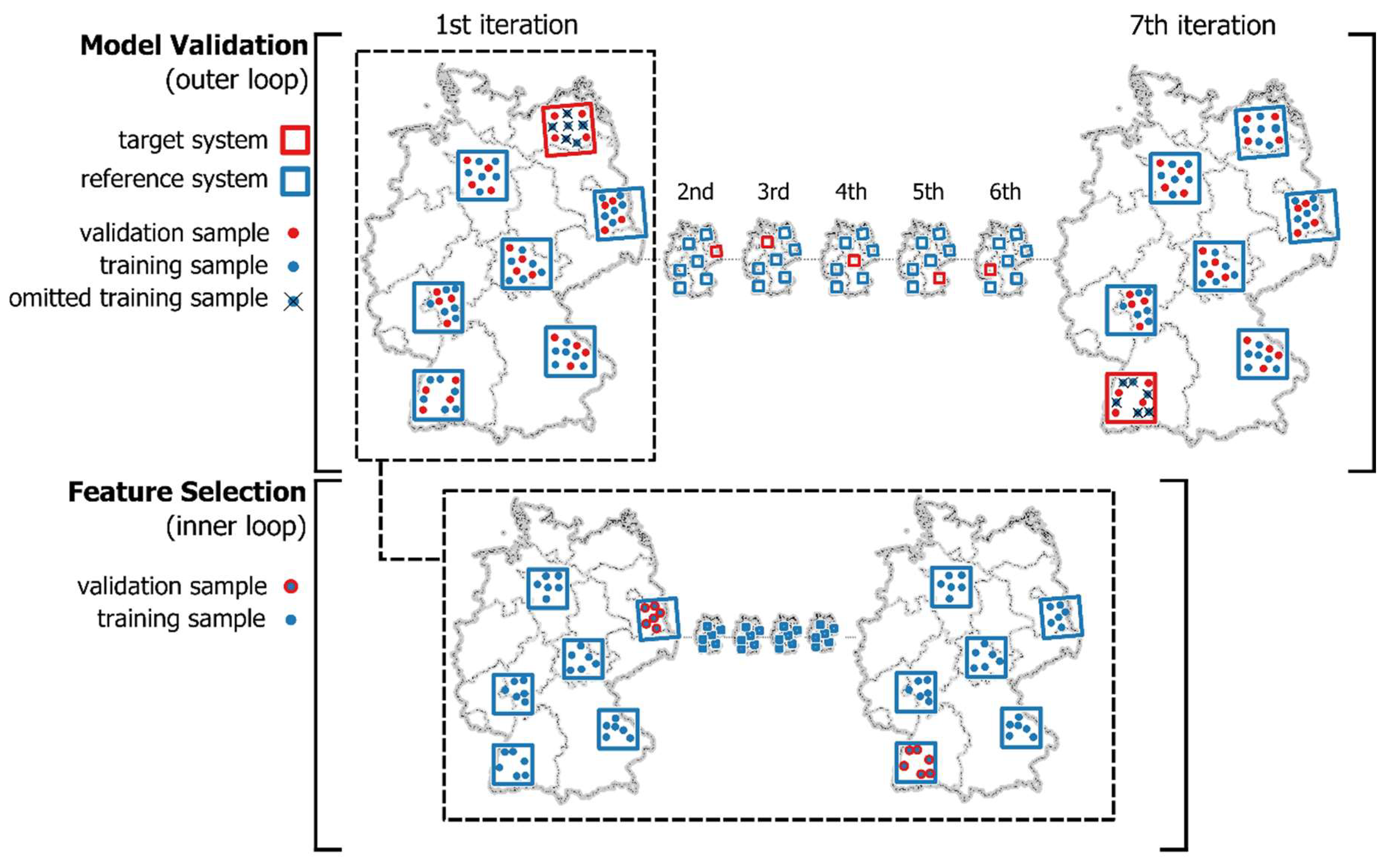
3.3. Model Performance Estimation Using Spatial Cross-Validation

To evaluate the models’ performance on a spatially independent test-set, we ran a 7-fold spatial CV where sample data from one study site was considered as one-fold (see Figure 4, ‘Model Validation’ part). In literature, spatial CV is also called leave-location-out CV [14] and block CV [15].

In each run of 7-fold spatial CV, the entire test data from one-fold is held out as an independent test-set representing the target system. The remaining six folds are used as a training site representing the reference system. After building the Random Forest model using training samples from the reference system, we spatially transfer the model to predict the test-set in the target system. Since we also want to evaluate the model’s performance in the training sites, we additionally predict the crop types for the test-set samples in the reference system. This procedure runs seven times; each time, the hold-out fold changes so that each fold is once the spatially independent test-set (target system) and six (k − 1) times the training-set (reference system).

We call the accuracy scores received from the reference system test-set samples ‘reference system accuracy’. The accuracy scores received from the target system test-set samples we call ‘target system accuracy’. The average and class-specific F1-scores (F1) were used as accuracy measures (Equation (4)). To better assess the quality of the model transfer to the target systems, we calculated the ‘accuracy loss’ (F1_loss) by subtracting the F1-score acquired from the reference system from the F1-score acquired from the target systems (Equation (5)).

$$\mathrm{F}1=\frac{\mathrm{True}\mathrm{Positive}\left(\mathrm{TP}\right)}{\mathrm{True}\mathrm{Positive}\left(\mathrm{TP}\right)+\frac{1}{2}\left(\mathrm{False}\mathrm{Positive}\left(\mathrm{FP}\right)+\mathrm{False}\mathrm{Negative}\left(\mathrm{FN}\right)\right)}$$

(4)

F1_loss = F1_{target system} − F1_{reference system}

(5)

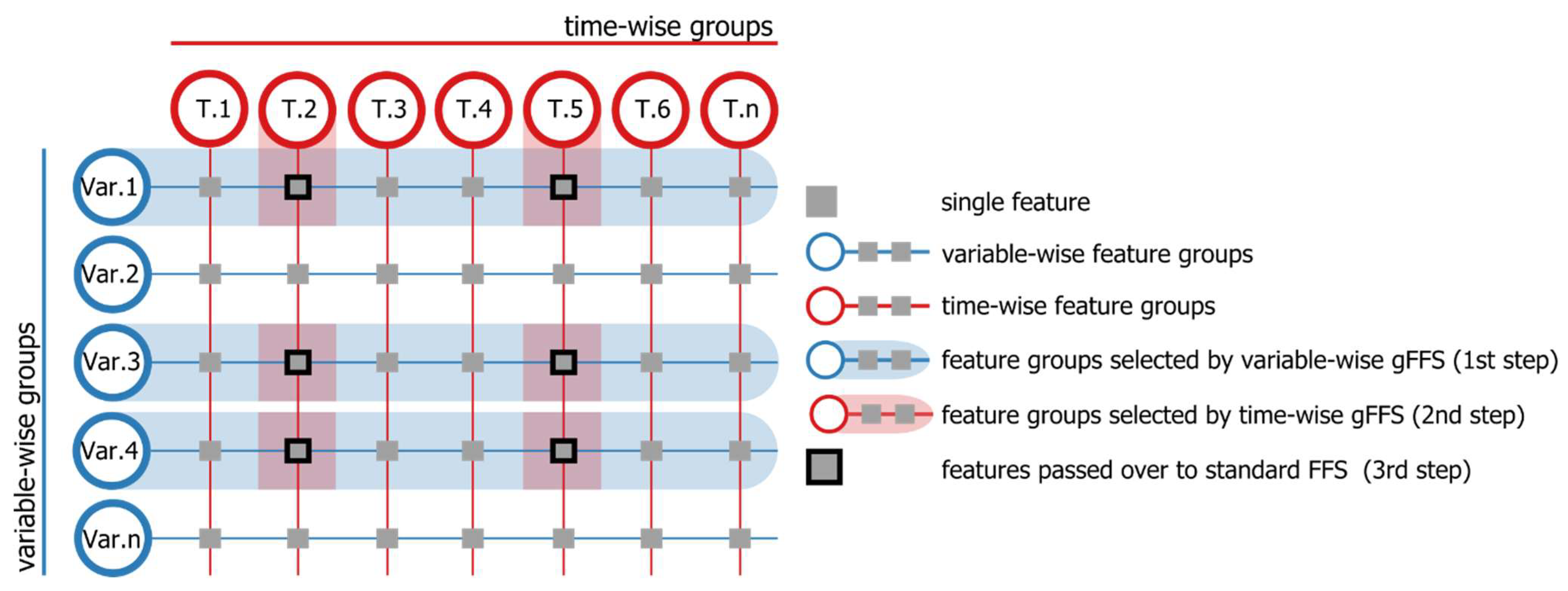
3.4. Feature Selection and Model Building

In reference systems, Random Forest models were built with the following two strategies: first by using all available features (‘All features’) and second by applying spatial feature selection (‘gFFS+sCV’). In total, we ran six experiments (see

Table 2. Overview of conducted six model building approaches with three input datasets and two feature selection approaches. For each experiment, the classification accuracies from the reference system (‘Ref.System’) and target system (‘Trg.System’) were recorded.

		Input Dataset
		S1 1	S2 2	S1+S2 3
Feature Selection Method	All features 4	Ref. System 6 and Trg. System 7	Ref. System 6 and Trg. System 7	Ref. System 6 and Trg. System 7
	gFFS+sCV 5	Ref. System 6 and Trg. System 7	Ref. System 6 and Trg. System 7	Ref. System 6 and Trg. System 7

¹ ‘S1’—SAR data from Sentinel—1 satellite; ² ‘S2’—optical data from Sentinel—2 satellite; ³ ’S1+S2’—combination of S1 and S2 by feature stacking; ⁴ ‘All features’—all features of input datasets were used to build the final Random Forest model; ⁵ ‘gFFS+sCV’—a subset of features selected using three-step group-wise Forward Feature Selection (gFFS) with spatial cross-validation (sCV) was used to build the final Random Forest model; ⁶ ‘Ref.System’—reference system is the system from which the training samples were used to build a model; ⁷ ‘Trg.System’—target system is the system from which no training samples were used. The target systems are only used to evaluate the classification performance of the models.

). We applied two feature selection approaches for each of only optical (‘S2’), only SAR (‘S1’) and the combination of optical-SAR (‘S1+S2’) datasets. The combination of optical and SAR features was performed by stacking features together. For each of conducted six experiments, we calculated reference and target system accuracy and classification accuracy losses by subtracting target system accuracy from reference system accuracy.

In ‘All features’, we selected all input features and all training samples from the six reference system folds to build final Random Forest models. The spatial feature selection was performed using a 3-step group-wise Forward Feature Selection (gFFS, described below). In ‘gFFS+sCV’, all training samples of the reference systems were split into six folds (see Figure 4, bottom) based on their spatial allocation (one study site = one spatial fold). The feature selection is then performed using gFFS and 6-fold spatial CV.

The final Random Forest model is then built using all reference system training samples and the selected feature subset. The Random Forest algorithm [38] was selected based on numerous reports of its successful application in crop type classification tasks [39,40], its ability to handle high dimensional feature spaces [41] and relatively low sensitivity to hyperparameter tuning [5]. The standard setting of the scikit-learn (version 0.22) implementation [42] of the Random Forest algorithm was used to build the final prediction models, with the only change in the number of trees from 100 to 500 as recommended in [41]. This hyperparameter setting is also commonly used among large-scale crop type mapping studies [3,43]. The square root of the total number of features was used to split the nodes in the single trees of this ensemble classifier.

Group-wise Forward Feature Selection (FFS) is a variation of standard Forward Feature Selection (FFS) [44] that begins by evaluating all single features individually. Here, by ‘evaluation’, we mean model building, predicting, and measurement of a performance score. After the first iteration, the input feature of the model with the highest performance score is selected as a fixed feature and passed to the next sequence. The procedure is reiterated by evaluating the set of fixed features from previous iterations together with one new feature from the remaining unselected features. The best-performing feature pair is fixed for the next iteration and subsequently again combined with each of the remaining features individually. The process runs until, e.g., no unselected features are left, the number of desired features is reached, or other custom stopping criteria are met.

One of the main limitations of FFS is its computational intensity. Intending to reduce the computational costs and still investigate all available features, we used group-wise FFS (gFFS) as presented in Orynbaikyzy et al. [20], based on Defourny et al. [45]. In gFFS, instead of considering single features within a given FFS iteration, groups of features were used.

The gFFS was conducted in three sequential steps (Figure 5). First, we run variable-wise gFFS, where features are grouped based on variables (e.g., complete time-series of S2 bands, vegetation indices, two S1 bands and their ratio). Each group of variables was considered as a single entity within gFFS. The feature groups selected by the variable-wise gFFS step then go to the second step—the time-wise gFFS. Here, the features are grouped based on time-steps (e.g., all features selected in the 1st step are from the 7th of June) and each group of time-steps was considered as a single entity within gFFS. The resulting selection of variable and time feature groups is then passed to the final third step, the standard FFS, where only single features are considered.

In the variable-wise gFFS, the number of groups varies between the two sensors. SAR data has six (VVasc, VVdsc, VHasc, VHdsc, VV/VHasc, VV/VHdsc), optical data has 13 (B2, B3, B4, B5, B6, B7, B8, B8A, B11, B12, NDVI, NDWI, NDYI), and consequently, the optical-SAR combination has 19 groups. In the time-wise gFFS, the number of groups is the same for both sensors and for their combination (29 time steps).

Feature selection was performed using the Random Forest [38] model with standard settings of scikit-learn implementation [42] of the algorithm but with 500 trees. Each of three gFFS procedures was stopped if adding a new feature or feature group did not increase the F1-score five times in a row. Open source Python packages such as MLxtend (version 0.17.2) [46], eo-box (version 0.3.10) [47], pandas (version 1.0.3) [48] and NumPy (version 1.18.1) [49] were used in the implementation of the presented 3-step gFFS.

4. Results

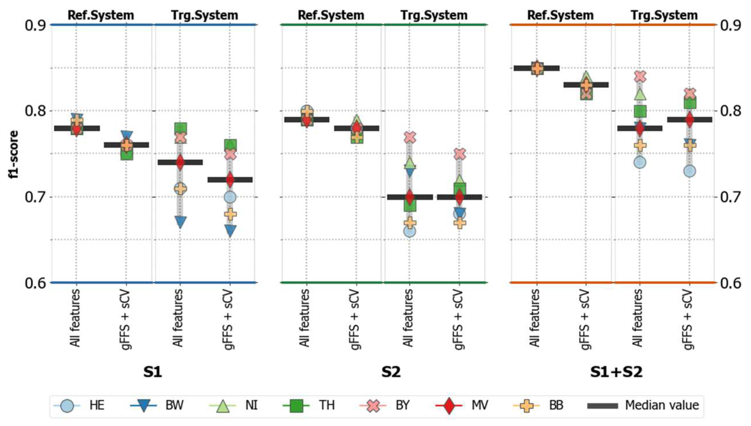
4.1. Overall Classification Accuracies

4.1.1. Accuracies without Spatial Transfer (Reference Systems)

Without considering a spatial transfer, the accuracies based on all features exceed those based on features selected using spatial gFFS (Figure 6, ‘Ref.System’). This pattern is common for all three feature sets. The highest median F1-score of 0.85 was reached with all features from optical and SAR sensors. The classification accuracies based on spatial gFFS showed lower median accuracies and higher accuracy ranges among reference systems, compared with the results using ‘All features’. On average, F1-scores were 0.02 lower, and the F1-score range (here, maximum-minimum) was reaching 0.03 of a difference.

The classification accuracies based on S1 features were marginally lower than those based on only S2 features when not considering spatial transfer; the difference of corresponding experiments never exceeded 0.05 F1-score.

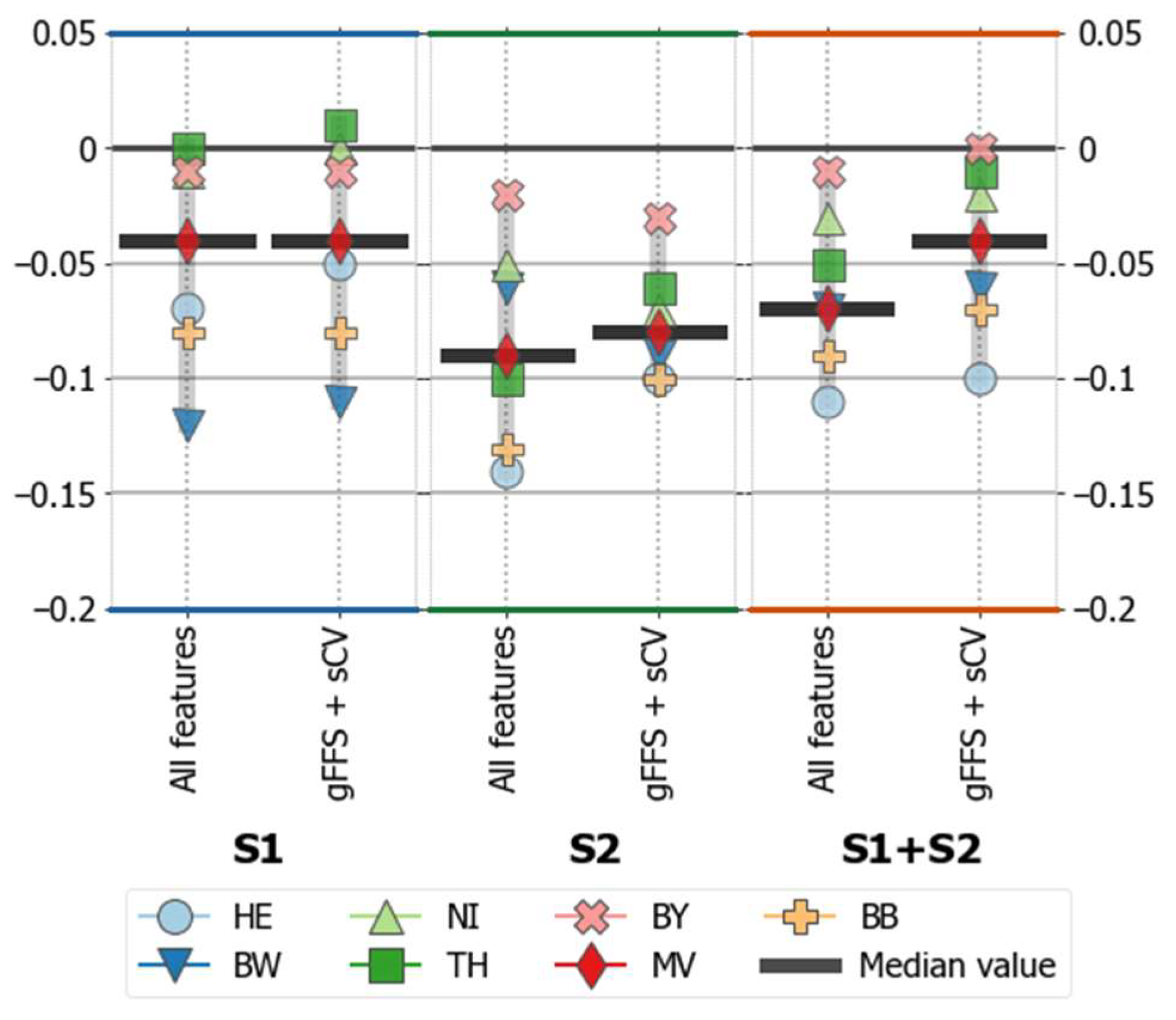
4.1.2. Accuracies for Spatially Transferred Models (Target Systems)

When spatially transferring the models (Figure 6, ‘Trg.System’), the highest median F1-score of 0.79 was reached with the combination of optical and SAR features selected using ‘gFFS+sCV’. But the median F1-score differences between no feature selection and spatial feature selection approaches remained below 3% for all sensor groups. The ranges of F1-scores in target systems are, on average, ten times higher than in reference systems. No distinct pattern was found indicating one approach’s superiority or inferiority in target systems.

Figure 7 shows that the highest average accuracy loss across all six experiments was observed in target tiles HE, BB, and BW (F1-score loss–−0.09). The lowest average F1-score reduction of 0.01 occurred in target tile BY.

The spatial transfer experiments based on S1 features showed higher accuracy values than those based on only S2 features (Figure 6). The lower accuracy losses in models based on S1 features and S1 + S2 were received compared to those based on S2 (Figure 7). The median F1-score loss with S1 features is −0.04. For S2 features, it equals −0.08, and for the combination of two sensors, it is −0.06. In the experiments with S1 + S2, performing spatial feature selection helped to reduce the average accuracy loss to 0.04 across the seven target systems.

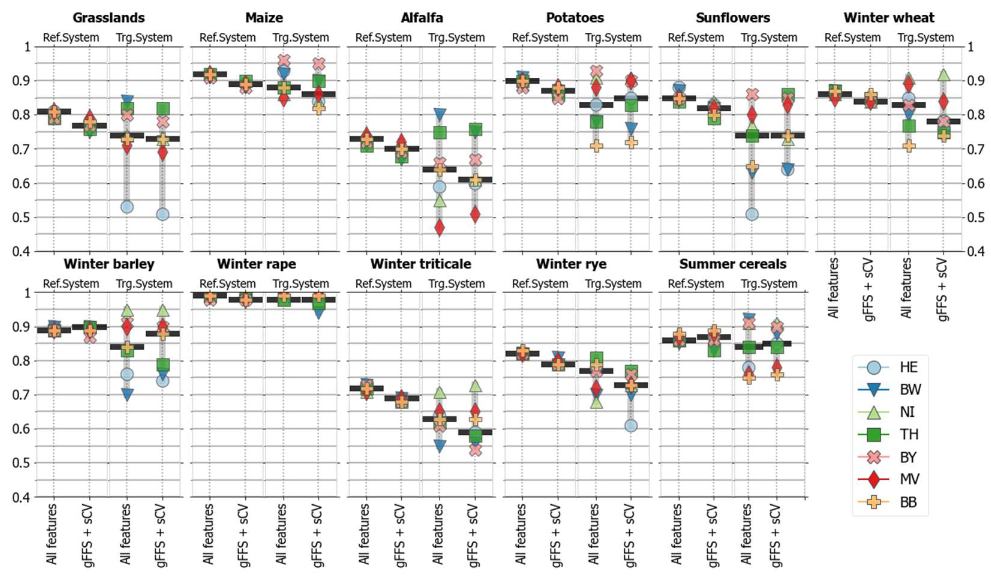
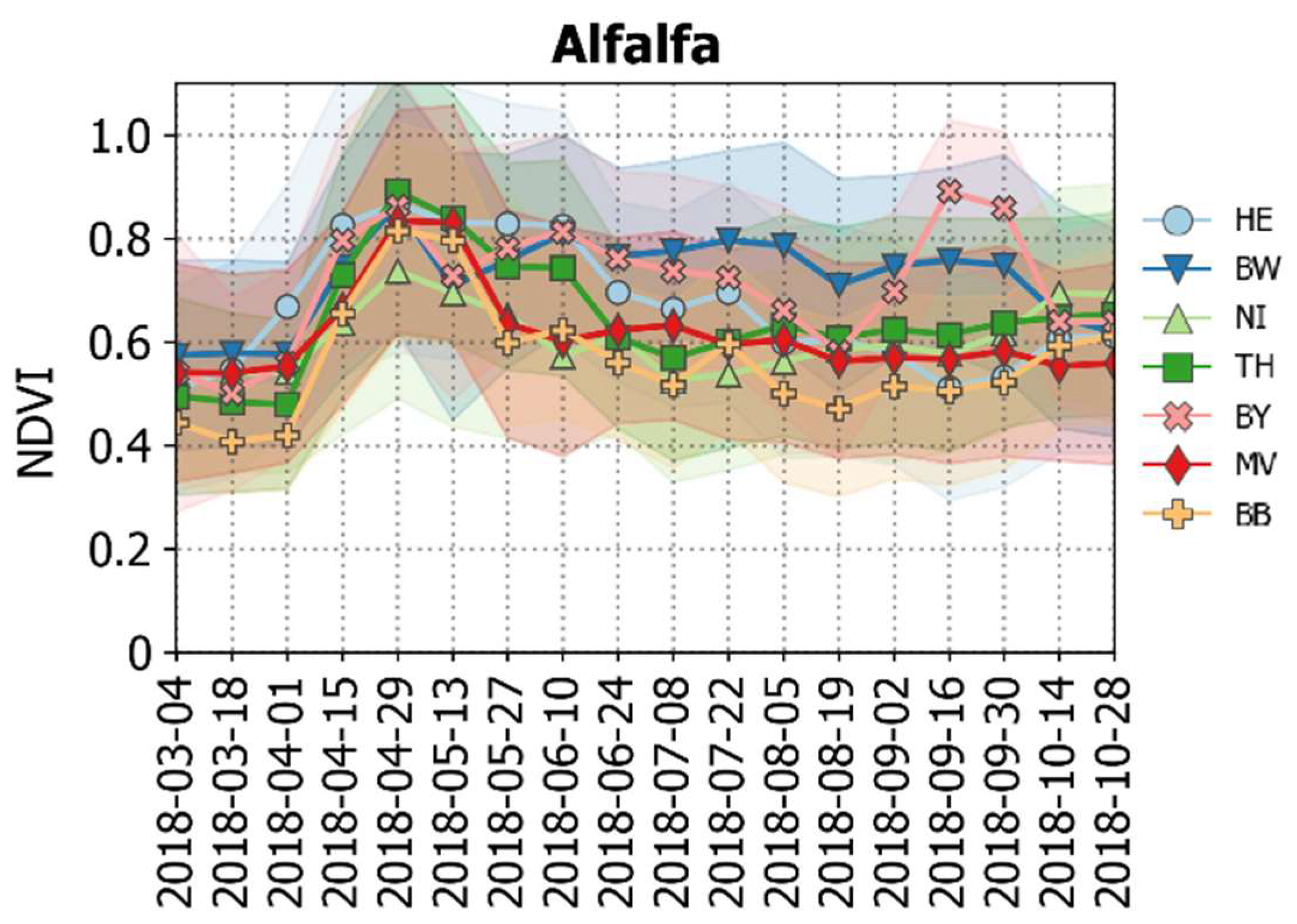
4.2. Class-Specific Classification Accuracies

4.2.1. Accuracies without Spatial Transfer (Reference Systems)

Without considering a spatial model transfer, class-specific accuracies were the highest when using optical and SAR features in combination (see supplementary material B). Except for summer cereals and winter barley, the highest median accuracies within the reference systems were reached when all features were used to build the models. In addition to Figure 8, we provide a table with median class-specific F1-scores for reference and target systems in supplementary material C.

The highest average range of F1-score values across the seven reference systems was observed for the class sunflowers (mean variation–0.06) and the lowest for the class winter rape (mean variation–0.01). Classification accuracies were higher for grasslands, maize, alfalfa, and summer cereals with only S2 features than with S1 or S1 + S2. For winter cereals, the difference in median F1-scores between runs based on S2 or S1 features did not exceed 0.05 for corresponding feature selection approaches. For a detailed plot with all six experiments, see supplementary material B.

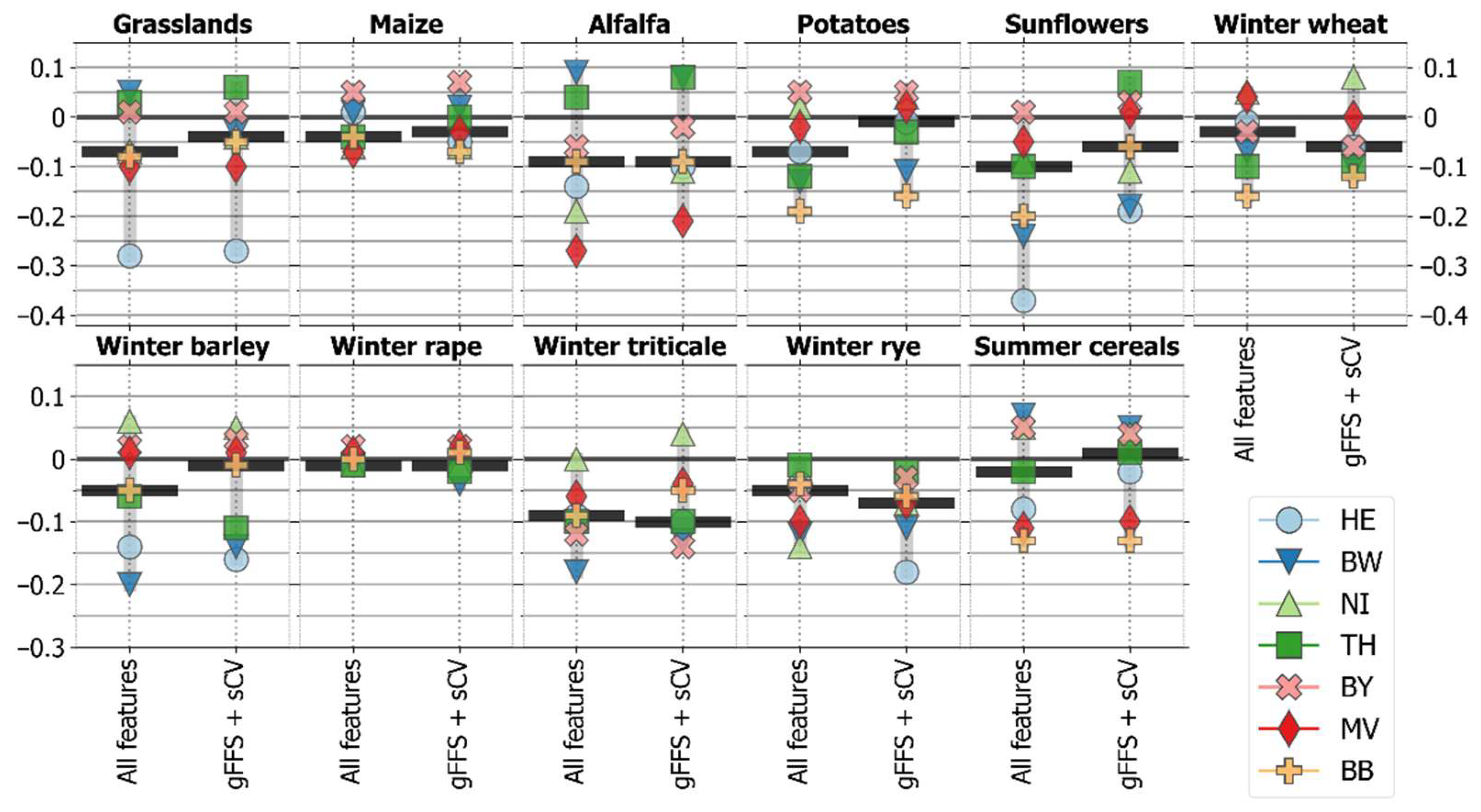
4.2.2. Accuracies for Spatially Transferred Models (Target Systems)

As in the reference systems, the average accuracy values in the target systems were the highest when we combined optical and SAR features (see Supplementary Material C). The potato and winter rape classes have shown equally high median accuracies with only S1 features as with features combinations (S1 + S2). In target systems, the average accuracy dropped for all classes except for winter rape when compared with the reference systems (Figure 9). For alfalfa, sunflowers, and winter triticale, the accuracy losses were most significant. The maximum F1-score losses for these three classes reached the following: −0.27 for alfalfa (target tile MV); −0.38 for sunflowers (target tile HE); −0.28 for winter triticale (target tile BW). Moreover, increased confusion among winter cereals and between alfalfa and grasslands was observed with ‘gFFS+sCV’.

The accuracy range (maximum-minimum) between the target systems was, on average, six times higher than that between the reference systems for the corresponding experiment sets (Figure 8). Among crop classes, the highest F1-score range across the seven target systems was observed for alfalfa (0.30), sunflowers (0.28), grasslands (0.27), and potatoes (0.21). For grasslands, the high variation resulted from tile HE, which showed a substantial accuracy loss when it is set as a target tile. Almost half of the grassland samples (84 samples) in target tile HE were misclassified as alfalfa, resulting in a very low F1-score.

The classes with high accuracy variations in the target systems also showed significant alteration of NDVI temporal profiles across the seven study sites. For example, alfalfa fields are harvested several times during the growing period, with varying harvest event patterns across the country. This results in various reflectance and backscatter patterns in the time-series and increases the within-class variance, which complicates the identification of the alfalfa fields (Figure 10). The NDVI temporal profiles for all considered crop classes and tiles are provided in Supplementary Material E.

Except for sunflowers and potatoes, no clear pattern was observed indicating the superiority or inferiority of a particular model building approach. For sunflowers and potatoes, the use of spatial feature selection on optical-SAR features reduced the median accuracy losses in target systems to 0.01 for potatoes (from an F1-score of 0.07 with ‘All features’) and 0.06 for sunflowers (from an F1-score of 0.10 with ‘All features’).

The models built using only SAR features showed the lowest accuracy losses in target systems for the following seven classes: grasslands, alfalfa, sunflowers, winter wheat, winter barley, winter rape, and winter triticale (Figure 9). The remaining four classes (maize, potatoes, winter rye, and summer cereals) showed the lowest accuracy losses with the combination of optical and SAR features.

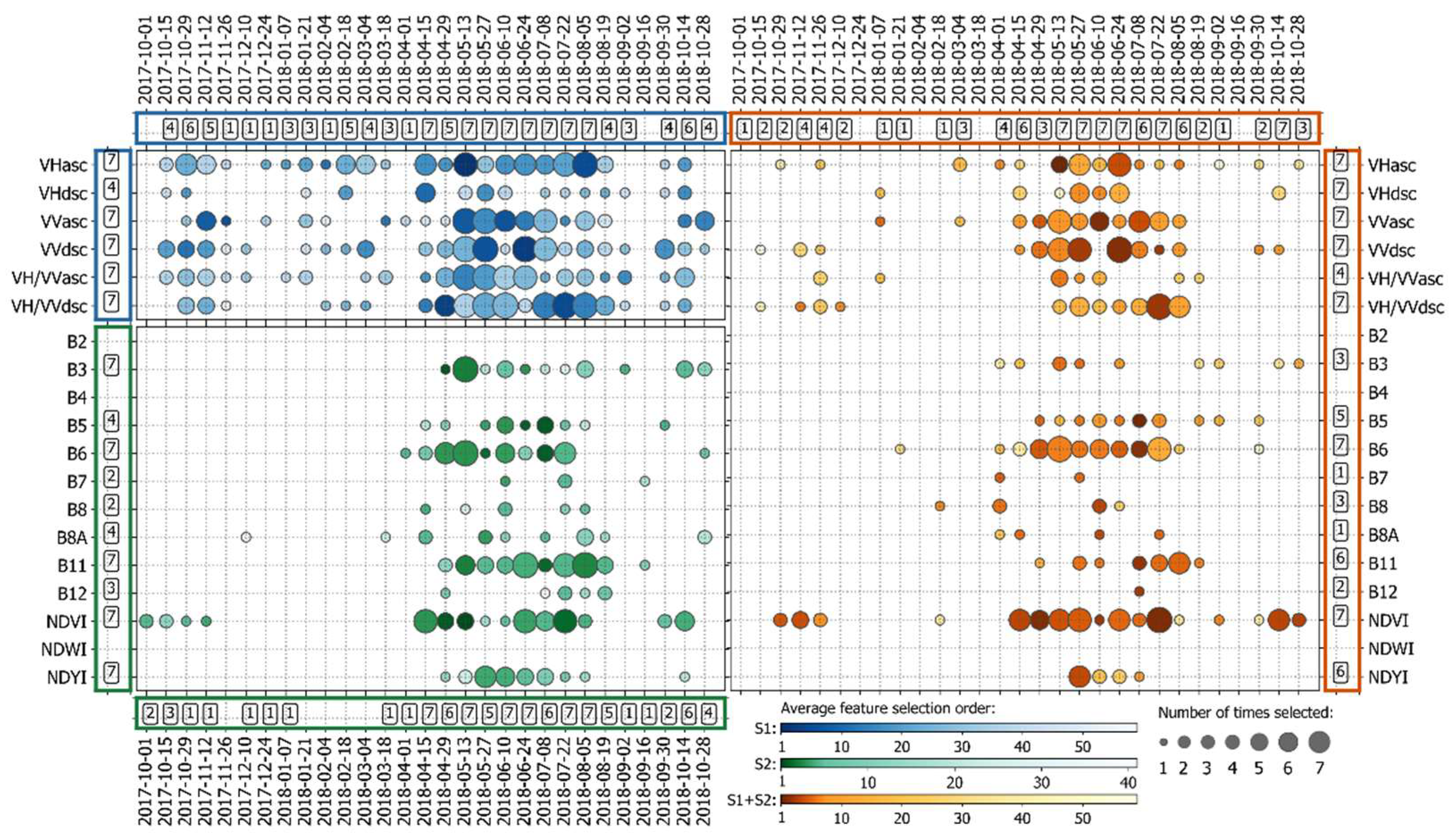
4.3. Features Selected with Spatial gFFS

For runs with only S2 features and S1+S2, the average number of selected single features was lower than with S1 features (

Table 3. The average number of selected single features or feature groups using 3-step group-wise Forward Feature Selection (gFFS) and the corresponding total number of model evaluation runs.

Sensors	Feature Selection Approach	Avg. Number of Selected Variable Groups	Avg. Number of Selected Time Groups	Avg. Number of Selected Single Variables	Total Number of Model Evaluation Runs	Number of Needed Runs If Standard FFS Applied
S1	All features	-	-	174	-	-
	gFFS+sCV	6	17	53	4474	7965
S2	All features	-	-	377	-	-
	gFFS+sCV	7	13	31	2807	11,568
S1 + S2	All features	-	-	551	-	-
	gFFS+sCV	11	14	46	6649	24,816

). The dissimilarities were present not only in the number of selected single features or groups but also in the repeatedly selected variables (Figure 11). Among optical variables, NDVI, NDYI, B6, and B11 were selected the most in the S2 and S1+S2 runs. All six SAR variables were selected more than four times in the S1 and S1+S2 runs.

The temporal groups covering the period from mid-April (15 April 2018) to the beginning of August (5 August 2018) were selected the most in all three sensor combinations. This period covers the most critical agro-phenological phases (e.g., plant emergence, plant height development, flowering) and land management activities (e.g., hay cut, harvest) across all study sites. The temporal groups in the two autumn seasons (autumn 2017, autumn 2018) were rarely selected with spatial CV.

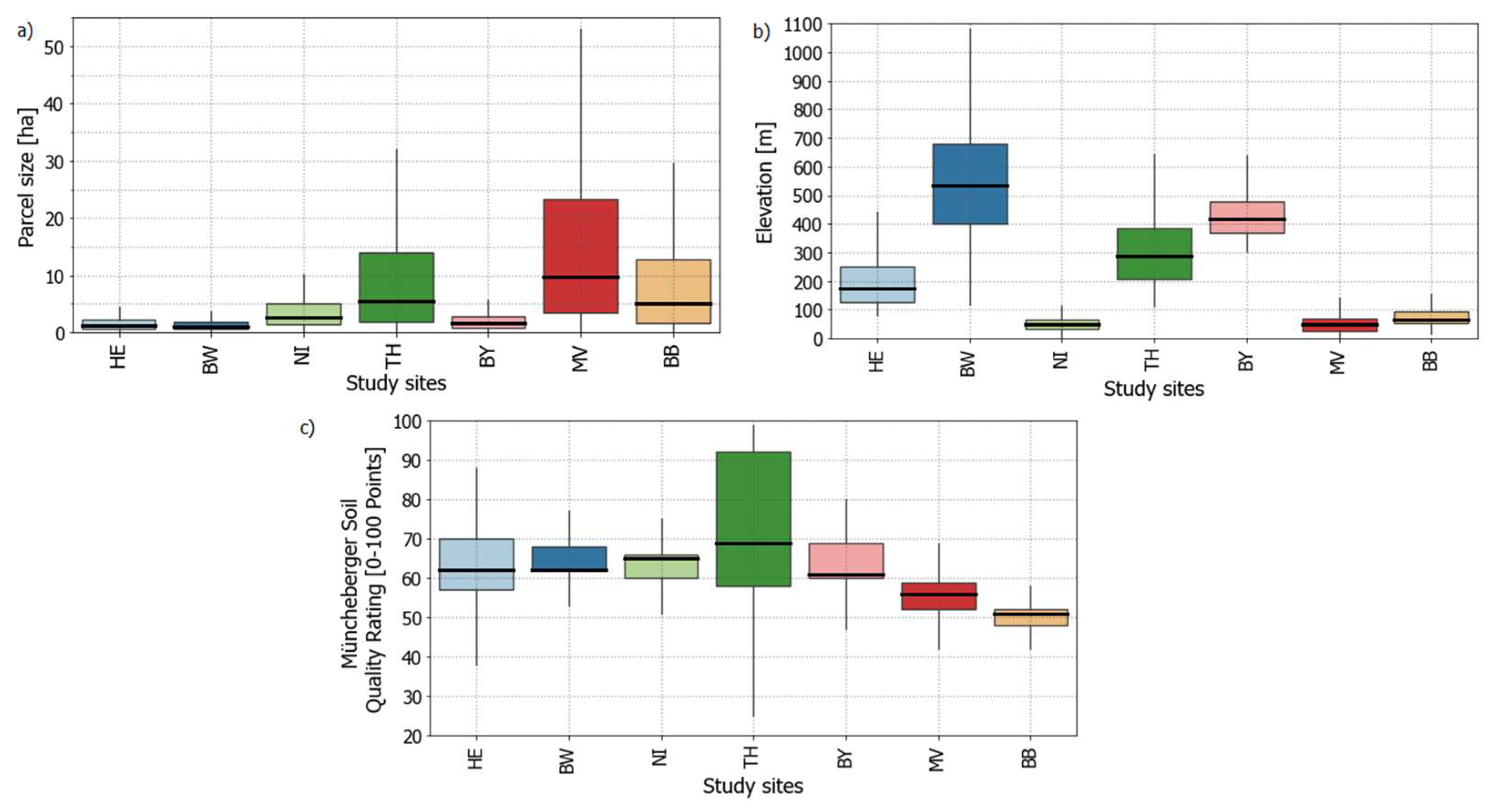
4.4. (Potential) Influences of Environmental Settings

As illustrated in Figure 12a, the sizes of the parcels in the study sites (MV, BB, and TH) located in Eastern Germany are bigger than those (BW, HE, NI, and BY) located in Western Germany. The smallest average parcel sizes were recorded in the southwestern two tiles—HE (1.2 ha) and BW (1.1 ha). These tiles showed high accuracy losses when a classification model built on all other regions was transferred to them. The parcel sizes also substantially vary depending on crop types (see Supplementary Material F). The crops with smaller average parcel sizes, such as grasslands and alfalfa, showed higher accuracy ranges when a model was spatially transferred to the unseen area than those crops grown on larger parcels.

Moreover, a considerable difference in surface elevation values is present across the study sites (Figure 12b). The highest average elevation was recorded for the tile BW, and the lowest elevation values were observed for three tiles located in the Northern German Lowlands (NI, MV, and BB). We observed considerable accuracy losses when Random Forest models were transferred to the tile BW.

The average values of the Müncheberger soil quality rating range between 60 and 70 points (Figure 12c), except for two northern tiles (MV, BB). The data from those two tiles showed the lowest average values, which indicate lower soil suitability for cropping purposes and potentially reduced plant vitality or biomass development. High accuracy losses were recorded when trained models were spatially transferred to those two northern tiles (Figure 7).

The temporal shifts in the timing of phenophases or field management activities (e.g., harvest) across the seven study sites can be observed from the phenological observation data acquired from DWD (Figure 13). For example, the average harvesting time for maize in tile BB happened approximately 3.5 days (minimum difference with tile MV) and 23 days (maximum difference with tile BW) earlier (Figure 13). When the Random Forest model was spatially transferred to tile BB, we obtained high accuracy losses for the maize class (see Figure 9). The same is true for summer barley, which is part of the summer cereals class (Figure 13). For winter wheat, notable temporal shifts (variation of median values: 27 days) were present in crop sowing events; For winter barley, higher dissimilarities were present in harvest time (17 days) than in the average timing of sowing events (8 days). The accuracy losses were higher for winter barley, with more temporal dissimilarities in harvest occurrence than for winter wheat (Figure 9). However, accuracy losses in the winter rape class were minimal despite similar differences in average harvest (14 days) and sowing (10 days) days across seven regions. More information is available in Supplementary Material G.

5. Discussion

Due to the environmental, climatic, and phenological differences across the study sites, classification accuracy losses in target systems are inevitable. While such regional differences and the lack of representative training samples are the main drivers of the reduced performance of Random Forest models in target sites, the quality and relevance of input remote-sensing features are other important aspects affecting the spatial transferability of the models. Our study demonstrated that the optical-SAR combination outperforms the classification results based on single sensors in both reference and target systems (Figure 6). The superior performance of the optical-SAR combination for crop type classification in model training sites is well known [18,21,39]. Our finding adds that the optical-SAR combination outperforms the single sensor datasets also in geographic spaces unseen by the model. A combination of optical and SAR features should be preferred when performing large-scale crop type mapping with spatially limited training data.

The classification accuracies of the models based on only optical features were marginally better than those based on only SAR features in the training sites (Figure 6). This goes in line with the available comparative literature on the application of optical and SAR data for crop type mapping [18]. However, in the target systems, it flipped to the opposite: models based on SAR features showed better accuracies than those based on optical. This resulted in lower accuracy losses with only SAR data compared to only optical, or a combination of both. This is a new finding that is relevant for real-world crop mapping scenarios where training data often has limited spatial coverage. It might be more important to select an approach or dataset that is more robust regarding spatial transferability than the best in the reference system.

The presented results show that the models built with SAR features are more robust (i.e., have lower accuracy losses in transfer systems) than optical or optical-SAR combinations. The majority of the investigations to date have reported SAR data’s suitability for crop type mapping in the training sites [50]. The results of our comparative study support the findings of [11] that SAR data is well suited for building spatially transferable crop type classification models and add that, in similar climatic conditions as in Germany, SAR-based models are more spatially transferable than those based on optical data. Recent studies from Woźniak et al. (2022) [51] and d’Andrimont et al., 2021 [52] illustrated that detailed mapping of crops at the country and continental scale with good accuracy is possible using only SAR data.

A reason for the lower accuracy losses of models based on SAR data could be the availability of consistent valid observations due to its all-weather sensing capabilities, which is crucial for successfully classifying various crops. Whereas the availability of valid optical data highly depends on the weather conditions of the sensed locations. For example, Ghassemi et al. (2022) [53] reported that generating monthly composites for the entire Europe was not possible due to the persistent cloud presence in some regions. Knowing that data from both sensors can successfully replicate the agro-phenological development phases of crops [22], it is reasonable that SAR-based models with more usable observations across large areas show better performance for spatial transfer than those based on optical data only. However, for areas with no persistent cloud cover issues, such spatial transferability study outcomes could be the opposite. Also, the capacity for spatial transferability of models based on only optical features could be different when other data compositing approaches are applied, as proposed by Preidl et al. [3], or a combination of two or more optical sensors is used, as shown by Griffiths et al. [2].

Contrary to the findings of [16] on small scale land use and land cover classification, performing spatial feature selection had no substantial effect on the spatial transferability of Random Forest models for crop type mapping. Nonetheless, spatial feature selection helped to eliminate irrelevant for the classifier features and to build much simpler models that are, based on the classification accuracies, comparable or even better (in the case of optical-SAR combination) than those based on all features. The models built using only eight percent from all single optical-SAR features (gFFS+sCV, Table 3) showed marginally improved absolute accuracies (Figure 6) and reduced accuracy losses (Figure 7) in target systems. Reduction of accuracy losses in target systems was also recorded for only optical features when spatial feature selection is applied (Figure 7). The models built with fewer predictor variables showed better spatial transferability as have already been reported by [13,54]. This underpins the relevance of spatial feature selection, especially for large-scale crop type mapping studies where an increased number of predictor variables decreases computational feasibility and requires substantial storage capacity.

As anticipated, accuracy losses vary among crop classes. Crops that are harvested several times during the growing period (e.g., grasslands and alfalfa), classes with a small number of parcels (e.g., sunflowers and potatoes), and classes with high genetic variability (e.g., wheat and rye) showed high accuracy losses in target systems. The survey of German farmers [55] indicated that the choice of cultivars is mainly driven by environmental variables such as soil quality. Consequently, this results in the spatially clustered representation of cultivars across the region, which could negatively affect a model’s ability to correctly predict the unseen cultivar. However, spatially transferring models for mapping of, e.g., maize and winter rape across large areas was possible with low accuracy losses. This supports the recent findings of Gilcher and Udelhoven [11] where acceptable spatial generalisation was possible for binary maize vs. non-maize classification with CNN. In future research, specific features designed to express generalised patterns, such as cutting event indicators that are independent of a specific moment in time, or various texture features based on optical and SAR data, should be considered for testing their usefulness for improving spatial transferability.

The spatial feature selection emphasised the importance of all SAR features along with NDVI, NDYI, B6 and B11. The relevance of NDVI, red-edge (B6) and short-wave infrared (B11) information for crop type mapping has already been reported in earlier studies [2,20]. In this study, NDYI from the May-June period, which corresponds to the rapeseed flowering phase in Germany, showed high importance. For mapping rapeseed crops with high accuracy, it is highly suggested to consider NDYI which has been also successfully applied for mapping rapeseed flowering events in Germany [32]. Contrary to the finding [56] where NDWI was among the top six important features, no NDWI features were selected in our study by spatial feature selection, indicating their irrelevance. As for SAR features, based on the outcomes of spatial feature selection (see Figure 11), we advise using a VH/VV ratio. The advantages of using the polarization ratio were reported by Veloso et al. [22] for separating maize and sunflowers during the flowering phase and by Inglada et al. [19] for early crop type mapping.

The results underpin that mapping dynamic land-use classes such as croplands at a larger scale without well-distributed training data is challenging and complex. Many abiotic and anthropogenic factors influence the development of the crops throughout the growing period [57]. Expectedly, those influencing factors enormously vary across geographic regions within Germany.

The variations in phenological crop development stages across the seven study sites (Figure 12) seem to be among the main drivers of the reduced spatial transferability of the tested Random Forest models. For example, due to a mild climate in the region of the upper Rhine valley (tiles HE and BW), winter crops reach maturity earlier [58] than in other regions of the country. In the German low mountain ranges (tile TH) and northern sites (tile MV), phenological development stages could occur later for a few days or even weeks. Phenological observation records presented in this study have shown considerable temporal differences in their occurrence across seven study sites. Consequently, when models are spatially transferred to the study sites with prominent differences in phenological development phases, the model will fail to predict crop labels accurately. Identifying an ‘area of applicability’ could be a potential approach to accounting for the fitness of the machine learning or deep learning models to new geographic areas for crop type mapping tasks [59].

The surface elevation varies substantially across the study sites (see Figure 12b). The tile BW with the highest average altitude (in sampled areas) above 500 m has also shown higher accuracy losses than other tiles. Similar results were reported by Stoian et al. [60], where higher misclassifications were recorded when models were spatially transferred to the high altitude zones with more complex topography. Besides shifts in phenology, in comparison to warmer lowlands, geometric distortions in the SAR data such as layover, foreshortening, shadow and high precipitation frequency (see Figure 2) in tile BW could have had a negative effect on the quality of SAR features in our study. This most likely explains the substantial accuracy losses in this tile when only SAR features are used.

Parcels sizes much smaller than those from the remaining tiles (Figure 12a) could have increased accuracy losses in the two southern tiles—HE and BW. As reported in earlier studies [61,62], small parcels are harder to classify due to the increased amount of mixed pixels and potential differences in field management. In our case, variations in farm management (e.g., seeding dates, management decisions) or type of farming [63] could be the reason for higher accuracy losses than the parcel sizes themselves.

The uneven spatial distribution of extreme drought in 2018 [27] combined with low soil quality (Figure 12c) could drive higher misclassification in tiles BB and MV. The north-eastern part of Germany is characterised by sandy soils and lower water holding capacities [35]. Thus, in severe drought events such as in 2018, these areas were often hit the hardest [64]. Especially, temperature-sensitive crops such as potatoes and sunflowers, and crops with high water demands, such as alfalfa, are among those most affected by drought. While the year 2018 was a particularly interesting case for evaluating the spatial transferability of the Random Forest models under varying climatic and environmental conditions, it would be beneficial to perform such a transferability analysis for other years with more typical climatic conditions across all study sites. Moreover, testing not only spatial but also temporal transferability of machine learning models using multi-sensor features and multi-year crop type information could advance our understanding of model transferability across space and time.

The study design was structured in the typical nested cross-validation manner where an outer loop is used for accuracy estimation using a spatially independent test-set while an inner loop is used for tuning the models via spatial feature selection (Figure 4). The training data distribution across Germany partially reflects the existing studies [2,3] where dense reference data is available for large areas but completely missing over other large areas, for example, entire federal states. In future studies, the permutation of not all study sites but all possible combinations (site-to-site transfer, 2 × 2 split) could be considered to better understand and maybe compensate for the reasons for accuracy losses in transfer regions.

The proposed 3-step gFFS method showed a good ability to select the relevant features with substantially reduced computational costs than the original Forward Feature Selection method. However, the main limitation of the proposed method is the risk of losing informative single features in omitted groups.

The accuracy losses were measured to assess the transferability and accuracy declines of the models in unseen geographic spaces by subtracting the F1-score acquired in the target system from that in the reference system. Here, F1-score values in each of the systems were based on the same number of validation points per crop type in each fold (tile). However, in studies with a varying number of samples for different crop types in the folds, the accuracy losses for the target system could be influenced by the dominant presence of ‘easy to predict’ (e.g., winter rape, maize) or small and complex crops (e.g., alfalfa, grasslands).

6. Conclusions

The presented research examines the spatial transferability of Random Forest models by analysing only optical, only SAR, and optical-SAR feature combinations, and testing if transferability could be improved by spatial feature selection. Based on the study outcomes, the following conclusions were drawn for our crop type mapping case in Germany:

• Random Forest models based on optical-SAR combinations outperform models based on single sensor data in training sites and geographic spaces unseen by the model;
• SAR-based models show the lowest accuracy losses when transferred to an area outside the training regions;
• Performing spatial feature selection on feature sets with only optical data and optical-SAR combination reduces classification accuracy losses in areas where the models were not trained;
• Small classes, grasslands, and alfalfa show high accuracy losses in areas outside the training regions;
• Environmental and geographic variables could aid in explaining or anticipating poor spatial transferability for specific regions.

Remote sensing data is undoubtedly one of the primary information sources for successful crop type mapping. Thus, understanding the strengths and weaknesses of different elements in classification approaches (e.g., datasets, derived features, and classifiers) with respect to spatial model transferability is an important issue, for those faced in practise with a situation where transferability is required.

References

1. Inglada, J.; Vincent, A.; Arias, M.; Tardy, B.; Morin, D.; Rodes, I. Operational High Resolution Land Cover Map Production at the Country Scale Using Satellite Image Time Series. Remote Sens. 2017, 9, 95. [Google Scholar] [CrossRef] [Green Version]
2. Griffiths, P.; Nendel, C.; Hostert, P. Intra-annual reflectance composites from Sentinel-2 and Landsat for national-scale crop and land cover mapping. Remote Sens. Environ. 2019, 220, 135–151. [Google Scholar] [CrossRef]
3. Preidl, S.; Lange, M.; Doktor, D. Introducing APiC for regionalised land cover mapping on the national scale using Sentinel-2A imagery. Remote Sens. Environ. 2020, 240, 111673. [Google Scholar] [CrossRef]
4. Lucas, B.; Pelletier, C.; Schmidt, D.; Webb, G.I. Unsupervised domain adaptation techniques for classification of satellite image time series. In Proceedings of the IGARSS 2020—2020 IEEE International Geoscience and Remote Sensing Symposium, Waikoloa, HI, USA, 26 September–2 October 2020. [Google Scholar]
5. Schratz, P.; Muenchow, J.; Iturritxa, E.; Richter, J.; Brenning, A. Performance evaluation and hyperparameter tuning of statistical and machine-learning models using spatial data. Ecol. Model. 2019, 406, 109–120. [Google Scholar] [CrossRef] [Green Version]
6. Nowakowski, A.; Mrziglod, J.; Spiller, D.; Bonifacio, R.; Ferrari, I.; Mathieu, P.P.; Garcia-Herranz, M.; Kim, D.-H. Crop type mapping by using transfer learning. Int. J. Appl. Earth Obs. Geoinf. 2021, 98, 102313. [Google Scholar] [CrossRef]
7. Gadiraju, K.K.; Vatsavai, R.R. Comparative analysis of deep transfer learning performance on crop classification. In Proceedings of the 9th ACM SIGSPATIAL International Workshop on Analytics for Big Geospatial Data, Seattle, WA, USA, 3 November 2020; Association for Computing Machinery: New York, NY, USA, 2020; Volume 1, ISBN 9781450381628. [Google Scholar]
8. Ajadi, O.A.; Barr, J.; Liang, S.-Z.; Ferreira, R.; Kumpatla, S.P.; Patel, R.; Swatantran, A. Large-scale crop type and crop area mapping across Brazil using synthetic aperture radar and optical imagery. Int. J. Appl. Earth Obs. Geoinf. 2021, 97, 102294. [Google Scholar] [CrossRef]
9. Bazzi, H.; Ienco, D.; Baghdadi, N.; Zribi, M.; Demarez, V. Distilling Before Refine: Spatio-Temporal Transfer Learning for Mapping Irrigated Areas Using Sentinel-1 Time Series. IEEE Geosci. Remote Sens. Lett. 2020, 17, 1909–1913. [Google Scholar] [CrossRef]
10. Lucas, B.; Pelletier, C.; Schmidt, D.; Webb, G.I.; Petitjean, F. A Bayesian-Inspired, Deep Learning-Based, Semi-Supervised Domain Adaptation Technique for Land Cover Mapping. Mach. Learn. 2021, 1–33. [Google Scholar] [CrossRef]
11. Gilcher, M.; Udelhoven, T. Field Geometry and the Spatial and Temporal Generalization of Crop Classification Algorithms—A Randomized Approach to Compare Pixel Based and Convolution Based Methods. Remote Sens. 2021, 13, 775. [Google Scholar] [CrossRef]
12. Hao, P.; Di, L.; Zhang, C.; Guo, L. Transfer Learning for Crop classification with Cropland Data Layer data (CDL) as training samples. Sci. Total Environ. 2020, 733, 138869. [Google Scholar] [CrossRef]
13. Wenger, S.J.; Olden, J.D. Assessing transferability of ecological models: An underappreciated aspect of statistical validation. Methods Ecol. Evol. 2012, 3, 260–267. [Google Scholar] [CrossRef]
14. Meyer, H.; Reudenbach, C.; Hengl, T.; Katurji, M.; Nauss, T. Improving performance of spatio-temporal machine learning models using forward feature selection and target-oriented validation. Environ. Model. Softw. 2018, 101, 1–9. [Google Scholar] [CrossRef]
15. Roberts, D.R.; Bahn, V.; Ciuti, S.; Boyce, M.; Elith, J.; Guillera-Arroita, G.; Hauenstein, S.; Lahoz-Monfort, J.J.; Schroder, B.; Thuiller, W.; et al. Cross-validation strategies for data with temporal, spatial, hierarchical, or phylogenetic structure. Ecography 2017, 40, 913–929. [Google Scholar] [CrossRef]
16. Meyer, H.; Reudenbach, C.; Wöllauer, S.; Nauss, T. Importance of spatial predictor variable selection in machine learning applications—Moving from data reproduction to spatial prediction. Ecol. Model. 2019, 411, 108815. [Google Scholar] [CrossRef] [Green Version]
17. Tuia, D.; Persello, C.; Bruzzone, L. Domain Adaptation for the Classification of Remote Sensing Data: An Overview of Recent Advances. IEEE Geosci. Remote Sens. Mag. 2016, 4, 41–57. [Google Scholar] [CrossRef]
18. Orynbaikyzy, A.; Gessner, U.; Conrad, C. Crop type classification using a combination of optical and radar remote sensing data: A review. Int. J. Remote Sens. 2019, 40, 6553–6595. [Google Scholar] [CrossRef]
19. Inglada, J.; Vincent, A.; Arias, M.; Marais-Sicre, C. Improved Early Crop Type Identification By Joint Use of High Temporal Resolution SAR And Optical Image Time Series. Remote Sens. 2016, 8, 362. [Google Scholar] [CrossRef] [Green Version]
20. Orynbaikyzy, A.; Gessner, U.; Mack, B.; Conrad, C. Crop Type Classification Using Fusion of Sentinel-1 and Sentinel-2 Data: Assessing the Impact of Feature Selection, Optical Data Availability, and Parcel Sizes on the Accuracies. Remote Sens. 2020, 12, 2779. [Google Scholar] [CrossRef]
21. Van Tricht, K.; Gobin, A.; Gilliams, S.; Piccard, I. Synergistic Use of Radar Sentinel-1 and Optical Sentinel-2 Imagery for Crop Mapping: A Case Study for Belgium. Remote Sens. 2018, 10, 1642. [Google Scholar] [CrossRef] [Green Version]
22. Veloso, A.; Mermoz, S.; Bouvet, A.; Le Toan, T.; Planells, M.; Dejoux, J.-F.; Ceschia, E. Understanding the temporal behavior of crops using Sentinel-1 and Sentinel-2-like data for agricultural applications. Remote Sens. Environ. 2017, 199, 415–426. [Google Scholar] [CrossRef]
23. Beck, H.E.; Zimmermann, N.E.; McVicar, T.R.; Vergopolan, N.; Berg, A.; Wood, E.F. Present and future Köppen-Geiger climate classification maps at 1-km resolution. Sci. Data 2018, 5, 180214. [Google Scholar] [CrossRef] [Green Version]
24. DWD. DWD Climate Data Center (CDC): Grids of Monthly Averaged Daily Air Temperature (2 m) over Germany, Version v 1.0. Available online: ftp://opendata.dwd.de/climate_environment/CDC/grids_germany/monthly/air_temperature_mean/ (accessed on 21 December 2020).
25. DWD. DWD Climate Data Center (CDC): Grids of Monthly Total Precipitation over Germany, Version v1.0. Available online: ftp://opendata.dwd.de/climate_environment/CDC/grids_germany/monthly/precipitation/ (accessed on 21 December 2020).
26. DWD The Weather in Germany in 2018. 2018, pp. 12–13. Available online: https://www.dwd.de/EN/press/press_release/EN/2018/20181228_the_weather_in_germany_2018.pdf%3F__blob%3DpublicationFile%26v%3D2 (accessed on 21 December 2020).
27. Reinermann, S.; Gessner, U.; Asam, S.; Kuenzer, C.; Dech, S. The Effect of Droughts on Vegetation Condition in Germany: An Analysis Based on Two Decades of Satellite Earth Observation Time Series and Crop Yield Statistics. Remote Sens. 2019, 11, 1783. [Google Scholar] [CrossRef] [Green Version]
28. Klages, S.; Heidecke, C.; Osterburg, B. The Impact of Agricultural Production and Policy on Water Quality during the Dry Year 2018, a Case Study from Germany. Water 2020, 12, 1519. [Google Scholar] [CrossRef]
29. Gerstmann, H.; Doktor, D.; Gläßer, C.; Möller, M. PHASE: A geostatistical model for the Kriging-based spatial prediction of crop phenology using public phenological and climatological observations. Comput. Electron. Agric. 2016, 127, 726–738. [Google Scholar] [CrossRef]
30. Hagolle, O.; Huc, M.; Desjardins, C.; Auer, S.; Richter, R. MAJA ATBD Algorithm Theoretical Basis Document. pp. 1–29. Available online: http://tully.ups-tlse.fr/olivier/maja_atbd/raw/master/atbd_maja.pdf (accessed on 21 December 2020).
31. Tardy, B.; Inglada, J.; Michel, J. Fusion Approaches for Land Cover Map Production Using High Resolution Image Time Series without Reference Data of the Corresponding Period. Remote Sens. 2017, 9, 1151. [Google Scholar] [CrossRef] [Green Version]
32. D’Andrimont, R.; Taymans, M.; Lemoine, G.; Ceglar, A.; Yordanov, M.; van der Velde, M. Detecting flowering phenology in oil seed rape parcels with Sentinel-1 and -2 time series. Remote Sens. Environ. 2020, 239, 111660. [Google Scholar] [CrossRef] [PubMed]
33. NASA. JPL NASA Shuttle Radar Topography Mission Global 1 Arc Second. 2013, Distributed by NASA EOSDIS Land Processes DAAC. 2013. Available online: https://lpdaac.usgs.gov/products/srtmgl1v003/ (accessed on 7 July 2021). [CrossRef]
34. BGR. The Product Center of the Federal Institute for Geosciences and Natural Resources (BGR). Available online: https://produktcenter.bgr.de/terraCatalog/Start.do (accessed on 9 June 2021).
35. Mueller, L.; Schindler, U.; Shepherd, T.G.; Ball, B.C.; Smolentseva, E.; Pachikin, K.; Hu, C.; Hennings, V.; Sheudshen, A.K.; Behrendt, A.; et al. The muencheberg soil quality rating for assessing the quality of global farmland. In Environmental Science and Engineering; Springer: Cham, Switzerland, 2014; pp. 235–248. [Google Scholar] [CrossRef]
36. DWD. Climate Data Center (CDC): Phenological Observations of Crops from Sowing to Harvest (Annual Reporters, Recent), Version v006. Available online: https://opendata.dwd.de/climate_environment/CDC/observations_germany/phenology/annual_reporters/crops/recent (accessed on 26 May 2021).
37. Tetteh, G.O.; Gocht, A.; Erasmi, S.; Schwieder, M.; Conrad, C. Evaluation of Sentinel-1 and Sentinel-2 Feature Sets for Delineating Agricultural Fields in Heterogeneous Landscapes. IEEE Access 2021, 9, 116702–116719. [Google Scholar] [CrossRef]
38. Breiman, L. Random Forests. Mach. Learn. 2001, 45, 5–32. [Google Scholar] [CrossRef] [Green Version]
39. Forkuor, G.; Conrad, C.; Thiel, M.; Ullmann, T.; Zoungrana, E. Integration of Optical and Synthetic Aperture Radar Imagery for Improving Crop Mapping in Northwestern Benin, West Africa. Remote Sens. 2014, 6, 6472–6499. [Google Scholar] [CrossRef] [Green Version]
40. Zhong, L.; Gong, P.; Biging, G.S. Efficient corn and soybean mapping with temporal extendability: A multi-year experiment using Landsat imagery. Remote Sens. Environ. 2014, 140, 1–13. [Google Scholar] [CrossRef]
41. Belgiu, M.; Drăguţ, L. Random forest in remote sensing: A review of applications and future directions. ISPRS J. Photogramm. Remote Sens. 2016, 114, 24–31. [Google Scholar] [CrossRef]
42. Pedregosa, F.; Varoquaux, G.; Gramfort, A.; Michel, V.; Thirion, B.; Grisel, O.; Blondel, M.; Prettenhofer, P.; Weiss, R.; Dubourg, V.; et al. Scikit-learn: Machine Learning in Python. J. Mach. Learn. Res. 2011, 12, 2825–2830. [Google Scholar]
43. Blickensdörfer, L.; Schwieder, M.; Pflugmacher, D.; Nendel, C.; Erasmi, S.; Hostert, P. Mapping of crop types and crop sequences with combined time series of Sentinel-1, Sentinel-2 and Landsat 8 data for Germany. Remote Sens. Environ. 2022, 269, 112831. [Google Scholar] [CrossRef]
44. Saeys, Y.; Inza, I.; Larrañaga, P. A review of feature selection techniques in bioinformatics. Bioinformatics 2007, 23, 2507–2517. [Google Scholar] [CrossRef] [PubMed] [Green Version]
45. Defourny, P.; Moreau, I.; Wolter, J.; Khalil, E.; Gallaun, H.; Miletich, P.; Puhm, M.; Villerot, S.; Pennec, A.; Lhernould, A.; et al. D33.1b-Time Series Analysis for Thematic Classification (Issue 2). Available online: https://www.ecolass.eu/project-deliverables (accessed on 19 February 2021).
46. Raschka, S. MLxtend: Providing machine learning and data science utilities and extensions to Python’s scientific computing stack. J. Open Source Softw. 2018, 3. [Google Scholar] [CrossRef]
47. Mack, B. EO-BOX: Open Source Python Package. Available online: https://github.com/benmack/eo-box (accessed on 8 June 2021).
48. McKinney, W. Data Structures for Statistical Computing In Python. In Proceedings of the 9th Python in Science Conference, Austin, TX, USA, 11–17 July 2010; pp. 51–56. [Google Scholar]
49. Oliphant, T.E. A Guide to NumPy; Trelgol Publishing: Spanish Fork, UT, USA, 2006. [Google Scholar]
50. Bargiel, D. A new method for crop classification combining time series of radar images and crop phenology information. Remote Sens. Environ. 2017, 198, 369–383. [Google Scholar] [CrossRef]
51. Woźniak, E.; Rybicki, M.; Kofman, W.; Aleksandrowicz, S.; Wojtkowski, C.; Lewiński, S.; Bojanowski, J.; Musiał, J.; Milewski, T.; Slesiński, P.; et al. Multi-temporal phenological indices derived from time series Sentinel-1 images to country-wide crop classification. Int. J. Appl. Earth Obs. Geoinf. 2022, 107, 102683. [Google Scholar] [CrossRef]
52. D’Andrimont, R.; Verhegghen, A.; Lemoine, G.; Kempeneers, P.; Meroni, M.; van der Velde, M. From parcel to continental scale—A first European crop type map based on Sentinel-1 and LUCAS Copernicus in-situ observations. Remote Sens. Environ. 2021, 266, 112708. [Google Scholar] [CrossRef]
53. Ghassemi, B.; Dujakovic, A.; Żółtak, M.; Immitzer, M.; Atzberger, C.; Vuolo, F. Designing a European-Wide Crop Type Mapping Approach Based on Machine Learning Algorithms Using LUCAS Field Survey and Sentinel-2 Data. Remote Sens. 2022, 14, 541. [Google Scholar] [CrossRef]
54. Ferraciolli, M.A.; Bocca, F.F.; Rodrigues, L.H.A. Neglecting spatial autocorrelation causes underestimation of the error of sugarcane yield models. Comput. Electron. Agric. 2019, 161, 233–240. [Google Scholar] [CrossRef]
55. Macholdt, J.; Honermeier, B. Yield Stability in Winter Wheat Production: A Survey on German Farmers’ and Advisors’ Views. Agronomy 2017, 7, 45. [Google Scholar] [CrossRef] [Green Version]
56. Sun, W.; Heidt, V.; Gong, P.; Xu, G. Information fusion for rural land-use classification with high-resolution satellite imagery. IEEE Trans. Geosci. Remote Sens. 2003, 41, 883–890. [Google Scholar] [CrossRef] [Green Version]
57. Bajocco, S.; Vanino, S.; Bascietto, M.; Napoli, R. Exploring the Drivers of Sentinel-2-Derived Crop Phenology: The Joint Role of Climate, Soil, and Land Use. Land 2021, 10, 656. [Google Scholar] [CrossRef]
58. Wizemann, H.-D.; Ingwersen, J.; Högy, P.; Warrach-Sagi, K.; Streck, T.; Wulfmeyer, V. Three year observations of water vapor and energy fluxes over agricultural crops in two regional climates of Southwest Germany. Meteorol. Z. 2015, 24, 39–59. [Google Scholar] [CrossRef]
59. Meyer, H.; Pebesma, E. Predicting into unknown space? Estimating the area of applicability of spatial prediction models. Methods Ecol. Evol. 2021, 12, 1620–1633. [Google Scholar] [CrossRef]
60. Stoian, A.; Poulain, V.; Inglada, J.; Poughon, V.; Derksen, D. Land Cover Maps Production with High Resolution Satellite Image Time Series and Convolutional Neural Networks: Adaptations and Limits for Operational Systems. Remote Sens. 2019, 11, 1986. [Google Scholar] [CrossRef] [Green Version]
61. Arias, M.; Campo-Bescós, M.; Álvarez-Mozos, J. Crop Classification Based on Temporal Signatures of Sentinel-1 Observations over Navarre Province, Spain. Remote Sens. 2020, 12, 278. [Google Scholar] [CrossRef] [Green Version]
62. Löw, F.; Duveiller, G. Defining the Spatial Resolution Requirements for Crop Identification Using Optical Remote Sensing. Remote Sens. 2014, 6, 9034–9063. [Google Scholar] [CrossRef] [Green Version]
63. Bichler, B.; Lippert, C.; Häring, A.M.; Dabbert, S. The determinants of the spatial distribution of organic farming in Germany. Ber. Uber Landwirtsch. 2005, 83, 50–75. [Google Scholar]
64. Lüttger, A.B.; Feike, T. Development of heat and drought related extreme weather events and their effect on winter wheat yields in Germany. Theor. Appl. Climatol. 2018, 132, 15–29. [Google Scholar] [CrossRef]
Figure 1. Location of the seven study sites in Germany.
Remotesensing 14 01493 g001
Figure 2. Mean monthly air temperature (top), monthly total precipitation (bottom) across the seven study sites from October 2017 to October 2018. Data source: German Weather Service (DWD).
Remotesensing 14 01493 g002
Figure 3. NDVI profile of original and interpolated values for the class potatoes (500 sample points) in tile HE.
Remotesensing 14 01493 g003
Figure 4. Graphical illustration of model validation and feature selection procedures. The pseudo-code of this workflow is provided in Supplementary Material A.
Remotesensing 14 01493 g004
Figure 5. 3-step group-wise Forward Feature Selection (gFFS) approach.
Remotesensing 14 01493 g005
Figure 6. Overall F1-scores of classifications based on three feature sets, with variants of using all features and spatial feature selection. The abbreviation keys are provided in Table 2.
Remotesensing 14 01493 g006
Figure 7. Classification accuracy (F1-score) losses in target systems compared to reference system accuracies for all six experiments based on three sensor inputs and two feature selection approaches. The abbreviation keys are provided in Table 2.
Remotesensing 14 01493 g007
Figure 8. Crop-specific classification accuracies (F1-score) in reference and target systems based on the optical-SAR combination and two feature selection approaches. The abbreviation keys are provided in Table 2. For a complete plot with three sensor groups, check supplementary material B.
Remotesensing 14 01493 g008
Figure 9. Crop-specific accuracy losses in the target systems for models using a combination of optical and SAR features (S1+S2). The abbreviation keys are provided in Table 2. For a complete plot with three sensor groups, check Supplementary Material D.
Remotesensing 14 01493 g009
Figure 10. NDVI temporal profile of class alfalfa across seven study sites.
Remotesensing 14 01493 g010
Figure 11. Analysis of feature selection results with spatial feature selection. The abbreviation keys are provided in Table 2. Outer boxes: The number of times a variable group (y-axis) or a time group (x-axis) was selected by spatial gFFS on runs with only SAR (blue borders), only optical (green border), and optical-SAR feature combinations (orange borders). Inner boxes: The single features, selected in the last step of spatial gFFS. The circle sizes represent the number of times a feature was selected, and the colour intensity represents the median order (sequence) at which it was selected.
Remotesensing 14 01493 g011
Figure 12. Distribution of (a) parcel sizes, (b) surface elevation, and (c) Müncheberger soil quality values among the seven study sites. Each boxplot contains all sampled 5500 points.
Remotesensing 14 01493 g012
Figure 13. Phenological phase observations for maize and summer barley (part of summer cereals class) located within the seven study sites (data source: DWD, 2018d). The following grouping of recorded phenological phases was applied: ‘Planting and emergence’ include ‘beginning of tilling sowing drilling’ and ‘beginning of emergence’ for maize; ‘Developing’ includes ‘beginning of flowering’, ‘beginning of mil ripeness’, ‘beginning of wax-ripe stage’, ‘yellow ripeness’, ‘tip of tassel visible’, ‘beginning of growth in height’ for maize and ‘beginning of heading’, ‘yellow ripeness’, ‘beginning of shooting’ for summer barley; ‘Harvesting’ includes ‘harvest’ for both classes. No observation was found for the ‘Planting and emergence’ stage for summer barley.
Remotesensing 14 01493 g013