A Machine Learning Snowfall Retrieval Algorithm for ATMS

Abstract

This article describes the development of a machine learning (ML)-based algorithm for snowfall retrieval (Snow retrievaL ALgorithm fOr gpM–Cross Track, SLALOM-CT), exploiting ATMS radiometer measurements and using the CloudSat CPR snowfall products as references. During a preliminary analysis, different ML techniques (tree-based algorithms, shallow and convolutional neural networks—NNs) were intercompared. A large dataset (three years) of coincident observations from CPR and ATMS was used for training and testing the different techniques. The SLALOM-CT algorithm is based on four independent modules for the detection of snowfall and supercooled droplets, and for the estimation of snow water path and snowfall rate. Each module was designed by choosing the best-performing ML approach through model selection and optimization. While a convolutional NN was the most accurate for the snowfall detection module, a shallow NN was selected for all other modules. SLALOM-CT showed a high degree of consistency with CPR. Moreover, the results were almost independent of the background surface categorization and the observation angle. The reliability of the SLALOM-CT estimates was also highlighted by the good results obtained from a direct comparison with a reference algorithm (GPROF).

1. Introduction

Snow is among the most important variables in the Earth’s climate. There are, in fact, several important effects of falling snow (snowfall) and snow at the surface on the climate system, as well as on the water cycle and the energy budget. The high albedo of snow is a primary factor controlling the amount of solar radiation absorbed by the Earth, affecting the surface energy balance as well as land–atmosphere interactions, and considerably influencing the atmospheric circulation. It should also be noted that snow has a primary role in the regional water cycle as the snow accumulated during the winter stores a large amount of freshwater, while the melting snow provides water resources for the ecosystem. Global monitoring of snowfall and snow cover is therefore of great relevance for climate change studies, for sustainable management of water and food resources, for understanding feedback mechanisms between hydrology and climate, and for forecasting hazardous weather and natural disasters such as floods and avalanches [1,2,3,4].

It is important to take into account the fact that snowfall is the most frequent type of precipitation in middle and high latitudes [5,6,7]; above 60–70 degrees it dominates over liquid precipitation [8]. At these high latitudes it is difficult to obtain reliable surface-based snowfall measurements due to the lack of dense networks of ground-based snow gauges and/or radars [9], and also due to the complex topography and extreme climatic conditions. Moreover, gauge-based measurements of snowfall, which are particularly challenging, can be largely unreliable as they are prone to wind-induced under-catchment errors [4,10,11].

These problems have highlighted the need to rely on satellite-based observations, which currently represent the most promising method of obtaining long-term global snowfall and snow-cover measurements. Spaceborne microwave sensors have been found to be particularly suitable for these purposes, unlike visible or infrared sensors which are used to analyze only the cloud-top features [12,13].

Thanks to the ability of microwaves (MWs) to penetrate clouds, passive MW radiometers have been widely used for snowfall detection [12,14,15,16,17,18,19,20,21,22,23]. In general, high-frequency channels (above 80 GHz) are more sensitive to scattering from ice hydrometeors, while lower-frequency channels (10–37 GHz) are more sensitive to surface emissivity [23,24,25,26]. Around this broad classification, several sensitivity studies have highlighted the potential of various high-frequency radiometer channels. For example, Bennartz and Bauer [27] investigated channels at 85, 150, and 183 GHz and highlighted the contribution of frequencies around 150 GHz to snowfall detection in middle and high latitudes. They also noted that channels near 85 and 183 GHz show potential for snow detection. Di Michele and Bauer [28] found that high-frequency bands (95–100, 140–150, 187 GHz) are the most suitable for the retrieval of snowfall over land and oceans. Skofronick-Jackson et al. [17] analyzed the contribution of the 166 GHz channel in detecting falling snow over land. You et al. [23] and Ebtehaj and Kummerow [22] highlighted the contribution of the combination of low- (10–19 GHz) and high-frequency (89–166 GHz) channels in snowfall detection. Edel et al. [29] analyzed the impact of measurements at 190.3 GHz and 183.3 ± 3 GHz for snowfall detection in the Arctic region.

In addition, dual polarization channels at high frequency, available from spaceborne conical scanning radiometers, have shown great potential for snowfall detection. Panegrossi et al. [30] studied in detail the sensitivity of the Global Precipitation Measurement (GPM) Microwave Imager (GMI) 166 GHz polarization difference for snowfall detection, showing that the polarization difference responds to moderate and heavy snowfall events. Kongoli et al. [31] examined the sensitivity of the 89 GHz and 166 GHz polarization differences to the snowfall intensity and evaluated their use for snowfall detection.

A fundamental contribution to the global estimate of snowfall is made by spaceborne active microwave sensors such as the Cloud Profiling Radar (CPR) on board CloudSat and the Dual-Frequency Precipitation Radar (DPR) on board the Global Precipitation Measurement-Core Observatory (GPM-CO). CPR (a 94 GHz nadir-looking radar) has proved highly effective in detecting snowfall with high sensitivity (~ –28 to –30 dBZ) and good orbital characteristics (sampling from 82°N–82°S latitudes) and has been widely used in snowfall research [3,5,32,33,34,35]. DPR (Ku 13.6 GHz and Ka 35.5 GHz) is also used in snow detection, although with different performances compared to CPR [2,36,37].

Despite the importance of falling snow and the considerable attention given by researchers to satellite snowfall retrieval, this is still one of the most challenging tasks. Compared to rainfall, snowfall retrieval from space is more challenging for several reasons related to the complex and dynamic interactions between the snowfall scattering signal and the surface. The non-spherical nature of ice particles and snowflakes, compared to roughly spherical raindrops, results in much more complex radiative properties [3,23]. Compared to rainfall, graupel, or hail, the snowfall scattering signal (and related depression of brightness temperatures -BTs) is much weaker, and therefore is more easily obscured by other contributions to the upwelling radiation (e.g., background surface or supercooled liquid water emission). Changes in the surface emissivity due to snow accumulation on the ground, snow wetness, and metamorphism, (altering the snow grain microstructure) can significantly impact the passive microwave signal and its relation to snowfall [3,23,38]. Moreover, several studies have shown that the snowfall scattering signal tends to be masked by the atmospheric water vapor and cloud liquid water emission in precipitating conditions [21,39,40]. In the study conducted by Panegrossi et al. [30], the impact of the presence of supercooled liquid water on the ability of GMI to observe snowfall at higher latitudes was analyzed in detail. The study showed how the influence of supercooled droplets on the high-frequency channels’ BTs is significant, especially when found on the top of ice cloud layers, and how their presence also affects the BTs’ polarization differences.

A field that is currently attracting the attention of researchers is the application of machine learning (ML) techniques to Earth observation. These machine learning techniques are widely applied in Earth observation because of their ability to approximate, to an arbitrary degree of accuracy, complex nonlinear and imperfectly known functions such as the relationships between satellite observations of the Earth and the state of the atmosphere and the surface [41,42,43,44,45,46,47,48,49,50,51]. A fundamental characteristic of these techniques is that the training process eliminates the need for a well-defined physical or numerical model that describes the relationships between the input values and output results, allowing the identification of these relationships during the learning phase. Interest in ML techniques is now also growing for parameter estimation related to snow, thanks to the increased availability of data, computational resources, and learning methods (e.g., deep learning).

Exploiting the potential of learning methods in both classification and regression analysis, several studies have been carried out to estimate snowfall and other snow-related parameters. Tedesco et al. [52] used the neural network approach in the retrieval of snow water equivalent, and snow depth, based on Special Sensor Microwave Imager (SSM/I) data. Tabari et al. [53] estimated snow depth and snow water equivalent using an improved neural network model. More recently, Rysman et al. [15,54] developed a machine-learning-based snowfall detection and retrieval algorithm for GMI (SLALOM) using CloudSat CPR coincident snowfall observations as a reference. The SLALOM algorithm is composed of random forest modules for the detection of snowfall and supercooled liquid clouds and a snowfall rate estimation module based on a gradient boosting approach. This study showed that the improvement in snowfall and high-latitude precipitation monitoring can be driven by machine-learning-based algorithms, exploiting concerted observations of active radars and passive microwave radiometers. Adhikari et al. [37] carried out a study to detect and estimate snowfall based on NOAA-18 Microwave Humidity Sounder (MHS) radiometer data, with CPR observations as a reference, using a random forest method. Tsai et al. [55] used a random forest classifier to map the total and wet snow-cover extent based on Sentinel–1 SAR radar data. Hicks and Notaros [56] described a method for the classification of snowflakes based on convolutional neural networks. Roebber et al. [57] presented a neural network approach to snowfall forecasting. Liu et al. [58] used a deep neural network for retrieving snow depth over sea ice in the Arctic basin, based on Special Sensor Microwave Imager and Sounder measurements.

The increasing number of operational cross-track scanning radiometers that will be on board polar orbiting satellites in the future (e.g., the Advanced Technology Microwave Sounder—ATMS—and the EUMETSAT Polar System program-Second Generation EPS-SG Microwave Sounder—MWS) will require dedicated efforts to study the potential of these radiometers to improve global snowfall monitoring. The goal of this paper is to present a new algorithm for snowfall detection and retrieval applied to ATMS measurements based on machine learning techniques (Snow retrievaL ALgorithm fOr gpM–Cross Track, SLALOM-CT). As in SLALOM, developed for GMI, CloudSat CPR products are used as a reference. In recent studies [15,30,48,54,59], the potential of the use of observational datasets built from coincident passive and active MW satellite observations for the development of satellite precipitation products has been shown. This approach differs from that based uniquely on simulations (a cloud resolving model coupled with a radiative transfer model), which was for a long time the only possible option for building a large, global cloud-radiation database [47,60,61,62,63,64,65]. The availability of the CPR observations has allowed the creation of observational databases, thereby reducing the limitations deriving from the assumptions of the simulations (e.g., the microphysical scheme of the cloud model, the emissivity of the background surface, and the scattering properties of ice hydrometeors) [21,25,66]. CPR, and the 2C-SNOW-PROFILE product in particular, has proven to be well suited to retrieving snowfall precipitation and very light rainfall [36]. However, since 2011, CPR has operated in daylight only mode, due to a battery anomaly, generating biases when CPR measurements are used to monitor global snowfall on relatively large time scales (daily or more), as recently investigated [67]. These effects, however, should not have a relevant impact on the results of this study, as only instantaneous estimates of snowfall rates and snow water path are used. Moreover, a recent study by Mroz et al. [68] compared several satellite-based snowfall estimates with the Multi-Radar Multi-Sensor (MRMS) radar composite over the continental United States, and the 2C-SNOW-PROFILE resulted in better agreement than any other product. These studies, however, confirmed some well-known limitations of 2C-SNOW-PROFILE, in particular the underestimation of the highest snowfall rates. Additionally, Mroz et al. [68] evidenced how passive microwave (PMW) snowfall retrieval (GPROF and SLALOM) is strongly affected by the presence of cloud liquid water. Moreover, Battaglia and Panegrossi [69], analyzing the CPR passive signal in the W band, evidenced how supercooled water is frequent in snowfall-producing clouds. Therefore, SLALOM-CT (as well as SLALOM) includes a module for the detection of supercooled liquid water droplets.

The SLALOM-CT algorithm was developed within the EUMETSAT Satellite Application Facility for Operational Hydrology and Water Management (H SAF) as part of the development of an operational day–1 precipitation product for the EPS-SG MWS mission.

The paper is structured as follows. Section 2 describes the dataset, focusing on the ATMS radiometer and the satellite product used in this research, together with a brief description of the machine learning techniques compared. Then, in Section 3, the SLALOM-CT algorithm architecture and the training procedure are described. Section 4 presents the results of the algorithm testing phase, including the analysis of the model selection. Moreover, in this section, the performances of each module composing SLALOM-CT are analyzed, in relation to the environmental conditions, and the results compared with the NASA GPM official ATMS product (GPROF-ATMS). Section 5 critically discusses the results of this work in the context of the recent literature, and finally, Section 6 summarizes the main results and draws the conclusions.

2. Materials and Methods

2.1. ATMS Radiometer

ATMS is a total power cross-track scanning microwave radiometer on board the Suomi National Polar-orbiting Partnership (NPP) satellite (and NOAA–20) with a swath of 2600 km and an angular span of ±52.77 relative to the nadir [70,71,72,73]. During each scan, the Earth is viewed from 96 different angles, sampled every 1.11°. ATMS has 22 channels, ranging from 23 to 183 GHz, providing both temperature soundings from the surface to the upper stratosphere (about 1 hPa, ~45 km) and humidity soundings from the surface to the upper troposphere (about 200 hPa, ~15 km). In particular, ATMS channels 1–16 provide measurements at microwave frequencies below 60 GHz and in an oxygen absorption band, and channels 17–22 are located at higher microwave frequencies above 89 GHz and in a water-vapor absorption band. The beamwidth changes with frequency and is 5.2° for channels 1–2 (23.8–31.4 GHz), 2.2° for channels 3–16 (50.3–57.29 and 88.2 GHz), and 1.1° for channels 17–22 (165.5–183.3 GHz) (see

Table 1. Characteristics of ATMS channels (https://www.star.nesdis.noaa.gov/jpss/ATMS.php, accessed on 2 February 2022).

Channel	Center Frequency (GHz)	EFOV Cross-Track (deg)	EFOV Along-Track (deg)	Polarization
1	23.8	6.3	5.2	QV
2	31.4	6.3	5.2	QV
3	50.3	3.3	2.2	QH
4	51.76	3.3	2.2	QH
5	52.8	3.3	2.2	QH
6	53.596 ± 0.115	3.3	2.2	QH
7	54.4	3.3	2.2	QH
8	54.94	3.3	2.2	QH
9	55.5	3.3	2.2	QH
10	57.29	3.3	2.2	QH
11	57.29 ± 0.217	3.3	2.2	QH
12	57.294 ± 0.32 ± 0.048	3.3	2.2	QH
13	57.29 ± 0.32 ± 0.022	3.3	2.2	QH
14	57.29 ± 0.32 ± 0.010	3.3	2.2	QH
15	57.29 ± 0.32 ± 0.0045	3.3	2.2	QH
16	88.2	3.3	2.2	QV
17	165.5	2.2	1.1	QH
18	183.31 ± 7	2.2	1.1	QH
19	183.31 ± 4.5	2.2	1.1	QH
20	183.31 ± 3	2.2	1.1	QH
21	183.31 ± 1.8	2.2	1.1	QH
22	183.31 ± 1	2.2	1.1	QH

for further details). The corresponding nadir resolutions are 74.78, 31.64, and 15.82 km, respectively. The outmost FOV sizes are 323.1 km × 141.8 km (cross-track × along-track), 136.7 km × 60.0 km, and 68.4 km × 30.0 km, respectively.

2.2. Satellite Products: CloudSat 2C-SNOW-PROFILE, DARDAR, and GPROF

In this study, reference values for the snow water path (SWP) and snowfall rate estimate (SRE) were obtained from the CloudSat snow profile product (2C-SNOW-PROFILE v.05A; [74]). This product provides estimates of the vertical profile of falling snow, such as snowfall rate, snow water content, and parameters of the snow size distribution. These estimates were retrieved, using an optimal estimation method [75], from the CloudSat CPR reflectivity profiles where snowfall was probable or certain (based on the classification of the 2C-PRECIP CPR product) and only for dry snow (i.e., a liquid water fraction less than 10–15%).

As a reference for the presence of supercooled liquid water droplets, the water phase mask provided by the DARDAR (liDAR + raDAR) product [76] was used. DARDAR, combining CPR radar and CALIOP lidar (on-board CALIPSO) observations, can estimate the cloud water phase and also the ice water content and ice particle effective radius, with a vertical resolution of 60 m and a horizontal resolution of 1.4 km (cross-track) × 1.7 km (along-track).

The results of the comparison of SLALOM-CT and the GPROF-ATMS product snowfall estimates (2AGPROFATMS) are also presented. GPROF is a physically based Bayesian precipitation retrieval algorithm used to deliver the official NASA GPM L2 precipitation products for all the GPM MW radiometer constellation including ATMS. It was originally proposed by Kummerow and Giglio [77], and since then it has continuously evolved towards a parametric approach that allows its use with different passive microwave sensors [78,79,80]. For this verification study, the 2A GPROF V05C for ATMS product was used.

2.3. The Coincidence Database

The algorithm was developed by exploiting a large dataset of coincident observations from a satellite-borne radar and radiometer (see

Table 2. Characteristics of the ATMS–CPR dataset.

Period	16/01/2014–31/08/2016
Geographical area	82°S–82°N, 180°W–180°E
Number of database points	6.5 M
Number of database points with snowfall	1.1 M
Horizontal resolution (km)	15.8 × 15.8 (nadir) 30 × 68.4 (scan edge)

). A coincidence dataset between ATMS and CPR observations was created. While ATMS provides integrated information on the surface and atmosphere characteristics of a large swath, CPR provides observations on the whole atmospheric column but with a very narrow swath (revisiting time of 16 days for a square of 100 km × 100 km). The current version of the coincident ATMS–CPR dataset was built considering a three-year (2014–2016) period of coincident (within 15 min) CPR reflectivity profiles and ATMS multichannel BT measurements.

In the database only the coincidences between the Suomi National Polar-orbiting Partnership (SNPP) satellite and CPR were considered, but for future studies it is planned to extend it by also considering the coincidences with the NOAA–20 satellite. The database incorporates some variables (see

Table 3. List of variables in the ATMS–CPR dataset.

Variables in the Database	Data Source
Latitude, Longitude (ATMS pixel)	NOAA–ATMS Sensor Data Record Operational
ATMS BTs	NOAA–ATMS Sensor Data Record Operational
Time of ATMS Pixel	NOAA–ATMS Sensor Data Record Operational
ATMS Scan Angle	NOAA–ATMS Sensor Data Record Operational
Supercooled Droplet	DARDAR (raDAR/liDAR) LATMOS—Reading Univ.
Snowfall Rate	2C–SNOW–PROFILE (CloudSat CPR product)
Snow Water Path	2C–SNOW–PROFILE (CloudSat CPR product)
Surface height	2B–GEOPROF (CloudSat CPR product)
Near-Surface Temperature	ECMWF Operational
Total Precipitable Water	ECMWF Operational
Freezing-Level Height	ECMWF Operational
Temperature Profile	ECMWF Operational
Relative humidity Profile	ECMWF Operational
Absolute humidity Profile	ECMWF Operational

) derived from the European Centre for Medium-Range Weather Forecasts (ECMWF) atmospheric model, which are used as ancillary inputs in the SLALOM-CT algorithm. These data include analysis (every 12 h) and forecasts (every 3 h) collected from the Operational Archive of the Meteorological Archival and Retrieval System (MARS). In detail, single-level variables were considered (near surface temperature—T_2m, total precipitable water—TPW, and freezing level height—FLH), together with vertical profiles of temperature, and relative and absolute humidity (i.e., selected from 14 pressure levels from 1000 to 1 hPa). The DARDAR-MASK product (from the Laboratoire Atmosphères, Milieux, Observations Spatiales—LATMOS—and the Cloud Group of the Department of Meteorology, University of Reading) was also used as a reference for the presence of supercooled liquid droplets.

It is worth noting that for the application of deep learning techniques, the database also includes information from the surrounding areas of each ATMS–CPR coincidence pixel. Each dataset element is made not of isolated points (single pixels) but of matrices (7 × 7 ATMS pixels “image”) around each ATMS–CPR coincidence pixel, as shown in Figure 1.

The database was built considering the horizontal resolution of the ATMS high-frequency channels (see Table 1). The CPR reflectivity profiles (and corresponding products, including DARDAR) falling within each ATMS IFOV were averaged with a Gaussian function approximating the ATMS antenna pattern (varying with the scan angle). Each CPR–ATMS coincidence pixel is therefore composed of a mean CPR profile (and associated products) associated with each ATMS BT vector. The ECMWF-model-derived variables were included into the dataset by selecting the forecast time step nearest the ATMS pixel and applying a bilinear interpolation in the horizontal plane. The dataset was further selected by removing all corrupted data and applying an additional filter based on the distance between each ATMS pixel and CPR, where all data with a minimum distance between CPR and the ATMS IFOV center greater than 22 km were removed.

2.4. The Machine Learning Techniques

2.4.1. The Random Forest Approach

The random forest, introduced by Breiman [81,82], is an ensemble learning algorithm that combines the ideas of “bootstrap aggregating (bagging)” and the “random subspace method” to construct randomized decision trees. The ensemble bagging technique is based on the use of multiple trees from random bootstrapped replicas of the learning dataset, in order to considerably enhance the classification accuracy over a single decision tree.

Each decision tree, trained in parallel, predicts an output, and each output is evaluated in the final response of the random forest. For the classification problem, the selection of the final output follows the majority voting system, and the output chosen by the majority of the decision trees becomes the final output of the random forest. For the regression problem, the final prediction is obtained by taking the mean of the output from various trees.

2.4.2. The Boosting Algorithms Approach

These ensemble algorithms are based on the boosting technique, which aims to obtain a robust classification/regression model by combining the responses of multiple weak learners. Weak learners are models that perform slightly better than random guessing; a commonly used type of weak learning model is the decision tree. In this technique, each sequential weak learner progressively learns from the classifications/regressions carried out incorrectly by the previous ones. In this way, a strong overall model can be built. Each weak learner is associated with a weight related to the total error in its prediction. The final prediction is obtained by taking into account the responses of all the weak learners, but each contributes with a different weight to the final decision.

AdaBoost was the first successful boosting algorithm, and the following boosting methods are based on similar techniques, with some differences, such as in the definition of the loss function to be optimized. Gradient boosting is a machine learning technique for regression and classification problems, using a gradient descent procedure to minimize the loss when adding trees.

Robust boosting is a technique that allows a better average accuracy to be produced in classification problems, with the result that it is more robust against label noise than AdaBoost.

2.4.3. The Shallow Neural Network Approach

A neural network consists of a number of neurons arranged in different layers, exchanging information with each other. Each layer holds a number of neurons determined, along with the number of layers, during the design of the network. Each node has its own transfer function (or activation function) and receives, as input, a weighted sum of the outputs of all the nodes of the previous layer. The output of the transfer function of each node is sent to all nodes in the next layer (fully connected network). The estimation of the weights of each neuron–neuron connection is performed in the NN training phase, during which a training database, providing the network with the inputs and the expected output, is used. The value of each weight is modified to reduce the error between the network and the expected outputs. At the end of the training, the network can approximate complex nonlinear and imperfectly known functions with an arbitrary degree of accuracy [83,84,85]. The final values of the weights connecting the neurons of the different layers store the knowledge of the NN. A detailed description of the NN design process can be found in Sanò et al. [86].

2.4.4. The Convolutional Neural Network Approach

The convolutional neural network (CNN), an important part of the deep learning technique, has proven to be very effective in the recognition and classification of images.

A CNN typically has three kind of layers: convolutional layers, pooling layers, and fully connected layers.

The convolutional layer is the main building block of the CNN and represents the greatest computational load. The convolution operation uses multiple filters that scan the entire image and extract features (feature map), preserving the corresponding spatial information. The convolution layer also includes a nonlinear operation called ReLU (rectified linear unit) which is used after each (linear) convolution operation for nonlinear amplification. The pooling level, computed immediately after a convolutional level, is used to reduce the size of the output of the convolutional level and to generate a condensed set of feature maps. Max pooling and average pooling are the commonly used pooling operations, but max pooling is the most common and is widely used. It consists of keeping only the maximum values of the feature maps, significantly reducing their spatial sizes and the processing effort in subsequent levels. The output of the convolutional and pooling layers, containing the high-level features of the input image, is sent to the fully connected layers, which constitute the last part of the CNN. The purpose of the fully connected layers, where every neuron in the previous layer is connected to every neuron in the next layer, is to use these features to provide the network output (e.g., the classification of the input image into various classes) [49,87,88,89,90].

Two convolutional network architectures, called VGG [91] and ResNet [92], were selected for this analysis. The flowcharts of the specific VGG and ResNet architectures tested are shown in Figure 2 and Figure 3. In both architectures, ReLU operations were used as transfer functions. A detailed description of the two convolutional network architectures can be found in the above-mentioned references. We only wish to highlight that the two chosen architectures differ in depth (i.e., the number of layers) and in the number of convolutional layers (3 in VGG and 19 in ResNet). Moreover, ResNet is characterized by the use of “residual blocks”, where the input and output of a sequence of two convolutional layers are connected by a “shortcut connection” that has been shown to be very effective for training very deep networks, avoiding degradation issues due to the depth [92].

3. The Algorithm

3.1. General Description of the Algorithm

The SLALOM-CT algorithm inherits and improves upon the scheme of SLALOM, developed for GMI. The SLALOM algorithm originally included three modules: one for the detection of snowfall, one for the detection of supercooled water droplets, and one for the estimation of the snow water path [15]. A fourth module for surface snowfall rate estimation was added to the algorithm [54]. An important difference in SLALOM-CT is related to this last module, which in the new version makes use only of the snow water path estimate and of some ancillary variables (without the use of BTs). For the first three modules, the two SLALOM versions share the same model-derived ancillary data and exploit the channels of the respective radiometers (GMI and ATMS). An important innovation in SLALOM-CT is the inclusion in the new algorithm of a surface classification scheme for the detection and classification of snow cover and sea ice at the time of the overpass [93]. The high-level algorithm flowchart is shown in Figure 4 and is composed of three main blocks:

• The input data block, which includes the pre-processing of BTs and ancillary variables and the surface classification at the time of the overpass (self-standing module);
• The classification block, which includes snowfall detection (SD) and supercooled droplet detection (SCD) modules;
• The estimate block, which includes one module for the retrieval of the snow water path (SPE module) and one for the retrieval of the surface snowfall rate (SRE module).

The algorithm takes as input the BTs from selected channels of the ATMS radiometer, ancillary information regarding the thermodynamic state of the atmosphere (from the ECMWF model operational forecast), and other variables regarding the state of the background surface, as listed below:

–

ATMS frequency channels’ BTs (channels 1–9, 16–22);

–

ECMWF ancillary variables (see Table 3);

–

Scan angle;

–

Surface height;

–

Dynamic surface map (from surface classification algorithm).

Regarding the exploitation of the ECMWF-model-derived variables, analogously to SLALOM [15], the two-dimensional variables T_2m, TPW, FLH, and surface elevation were used as input to the modules, while the first four principal components of temperature and humidity (relative and absolute) profiles were used.

The dynamic surface map is based on the PESCA algorithm [93], which allows for the detection and classification of frozen surfaces (sea ice and snow cover) at the time of the satellite overpass. This algorithm is based on a single decision tree module based on low-frequency ATMS BTs (23.8, 31.4, and 88.2 GHz channels) and some model-derived variables (TPW and T_2m). Over land, PESCA is able to discriminate between snow-free land and four classes of snow-covered surfaces: Thin Snow and Deep Dry Snow are built from seasonal snow and differ mainly in their thickness, and Perennial Snow and Polar Winter Snow are found at higher latitudes (the first over the whole year and the latter mainly in winter in central Greenland and Antarctica). Over the ocean, PESCA classifies the surfaces into Ice-Free Ocean, Broken Sea Ice (where the satellite FOV is partially covered by sea ice), New Year Ice (built from recently formed sea ice) and Multilayer Ice (thick and older sea ice). The algorithm has shown very good performance within some environmental limits (i.e., TPW < 10 kg m⁻² and T_2m < 280K). When these conditions are not met, the surface is categorized as either “Land Uncertain” or “Ocean Uncertain”. A further class is defined as Coastal Areas where the ATMS IFOV includes both land and ocean.

All the inputs feed the classification block consisting of the snowfall detection (SD) and supercooled droplet detection (SCD) modules.

The BTs and the corresponding ancillary data for pixels that are classified as “snowfall” by the SD module form the input of the snow water path estimation module (SPE). The SPE output (snow water path in kg/m²) feeds the SRE module that produces snowfall rates in mm/h.

The information on the presence of supercooled droplets, associated with the snow water path and snow rate estimates, allows the conditions under which the retrieval is less reliable to be identified. A supercooled droplet layer on top of a snow cloud can mask the scattering signal of the snowflakes below [30].

3.2. Training and Optimization of the Machine Learning Modules

During the preliminary analysis of the algorithm’s performance, it was highlighted that a relevant role in the surface snowfall rate estimation is played by the SD and the SPE modules. Accordingly, the algorithm development mostly focused on the optimization of the SD and SPE modules.

The SD and the SPE modules underwent an extensive intercomparison process between various machine learning techniques. In particular, for the SD module and SPE module, a random forest, various gradient boosting algorithms (AdaBoost [94], RobustBoost [95] and least-squares boosting [96]), a shallow neural network, and two convolutional network architectures (VGG and ResNet) were tested.

The CPR–ATMS coincidence dataset, described in Section 2.3 and spanning 3 years (2014–2016) was divided into two independent datasets: a training dataset (1 year long) and a testing dataset (2 years long). The training and testing datasets were carefully quality controlled and built following different criteria to take into account SD and SPE problems. In particular, for the SPE only, observations with a surface snowfall rate greater than 0 mm/h were used in training and testing, while the SD training and testing were based on all observations (with and without snowfall) with a FLH lower than 500 m. It has been observed that only a negligible fraction of observations are associated with snowfall when the FLH is beyond this threshold.

Another aspect to highlight in the building of the training and testing datasets is that convolutional neural networks are suited for retrieval problems involving images, while the other machine learning techniques tested in this research are pixel-based, i.e., each pixel, independently of the relative position in the original observation, is treated as stand-alone. In order to directly compare the results from the pixel-based and image-based ML techniques, the datasets are composed of several features (or input variables, or channels) from a 7 × 7 image of adjacent pixels. The target variables (output of the ML algorithm) are taken only from the central pixel of the 7 by 7 feature image. In the training and in the application of the image-based convolutional networks, the full feature image is used as input, while for the pixel-based ML techniques only the central pixel of each channel is used as input. We should note that this approach could limit the potential of convolutional neural networks for solving our problems; however, it allows a direct comparison of the pixel- and image-based ML techniques and permits quantification of how the pixels surrounding the central pixel can contribute to the solution of the retrieval problem.

Each ML technique was optimized during the training by varying several structural and tuning parameters. This approach implied the training of a very large number of ML algorithms. In particular, for random forest, the ensemble trees algorithms were trained by optimizing the number of trees, the number of splits per tree, and the minimum leaf size, while in the gradient boosting algorithm the number of training epochs, the number of splits per tree, the initial learning rate, and the robust error goal (only for the RobustBoost algorithm) were optimized.

The resulting optimized algorithms showed significant differences from each other. The random forest algorithms are characterized by a relatively low number of very deep trees (e.g., 200 trees composed of 10,000 splits in SPE). In contrast, the gradient boosting algorithms are built with a very large number of very simple trees (e.g., 2000 trees with 5 splits each for the SPE). Moreover, in the training of the neural networks, both shallow and deep, various structural parameters were optimized (i.e., number of layers and number of perceptrons or weights), together with several training parameters (i.e., initial learning rate, square gradient decay factor, and regularization-related parameters). During the training, the mean squared error and cross entropy were used as loss functions for the regression and classification networks, respectively, for both shallow and convolutional architectures. The resulting optimized shallow neural networks were composed of two hidden layers of 50 and 25 perceptrons for both SD and SPE. Finally, the structural characteristics of the optimized VGG and ResNet convolutional networks are shown in Figure 2 and Figure 3.

As already mentioned, the accuracy of the snowfall rate estimate strongly depends on the quality and accuracy of the snow water path that feeds the snowfall rate estimate module. In particular, it was noted that a relatively simple shallow neural network can reproduce the CPR snowfall rate near to the surface very effectively if it is trained using the CPR SWP and some ancillary environmental variables (T_2m, TPW, surface elevation, and the first four principal components of temperature and humidity—relative and absolute—profiles). A two-hidden-layer (with 50 and 25 perceptrons) shallow neural network was trained using the SWP derived from the CPR 2C-SNOW-PROFILE product and the previously cited environmental variables. This NN (called SRE-CPR) reproduces the CPR snowfall rate near to the surface with an RMSE of 0.063 mm/h (corresponding to a coefficient of determination—R²—of 0.84). Therefore, if the SPE module reproduces the CPR SWP adequately well, the SRE module can be based only on SWP and environmental variables. Consequently, the development efforts were focused on the training of a very effective SPE module. The final SRE module consisted of a shallow neural network (identical in structure to SRE-CPR) that uses as input the SWP derived from the SPE module (details are reported in Section 4.2). Finally, the SCD module was composed of a shallow neural network very similar to the one for the SD module (i.e., 50 and 25 perceptrons in the two hidden layers).

For the training and optimization phases of the different ML modules, the “Statistics and Machine Learning Toolbox” and the “Deep Learning Toolbox” of MATLAB 2021b were used.

4. Results

4.1. Intercomparison of Machine Learning Techniques

Table 4. SWP estimation statistics.

	Random Forest	Gradient Boosting	Shallow NN	VGG	ResNet
RMSE [kg/m2]	0.078	0.090	0.050	0.055	0.072
R2	0.667	0.553	0.861	0.834	0.714
ME [kg/m2]	−3.66 × 10−3	−1.08 × 10−2	−1.59 × 10−5	−5.61 × 10−5	−1.2 × 10−3
Corr	0.86	0.83	0.93	0.92	0.87
N0	4 × 106	104	3 × 104	7 × 104	4 × 106

shows the results for the intercomparison of the ML techniques used for the SWP estimate in the test dataset (2014 and 2016). The analyzed statistics include the root mean squared error (RMSE), the coefficient of determination (R²), the mean error (ME), the Pearson’s correlation coefficient (Corr), and the number of trained parameters (N₀). R² is defined as:

$${\mathrm{R}}^2=1-\frac{{\mathrm{RSME}}^2}{{\mathrm{STD}}^2}$$

(1)

where STD is the SWP standard deviation in the dataset. All ML techniques show a very low mean error and a relatively high correlation. The RMSE is also limited. Two algorithms (the two based on the simpler neural networks) outperformed the others. In particular, the shallow neural network showed an RMSE of 0.050 kg/m², corresponding to an R² of 0.86, our best result, while the VGG showed statistics quite similar to the shallow neural network but slightly worse (RMSE of 0.055 km/m² and R² of 0.83). Both tested tree-based algorithms (random forest and gradient boosting) showed worse performances. The ResNet algorithm showed better results than the tree-based algorithms, but they were suboptimal with respect to the simpler neural networks. N₀, reported in the last line of Table 4 as a proxy to quantify the complexity of the algorithms, indicates the number of tests, splits, or weights of each algorithm. Some conclusions can be drawn from this analysis: (1) neural networks show a higher capability for solving the problem of SPE than tree-based algorithms; (2) in this case the image-based approach, which considers the pixels surrounding the central pixel, makes no contribution to the solution, as the pixel-based shallow neural network outperforms every other algorithm tested; (3) ResNet is too complex for the size of our training dataset. Based on this analysis the shallow neural network algorithm was chosen for the SPE module of SLALOM-CT

Table 5. Snowfall detection statistics.

	Random Forest	RobustBoost	AdaBoost	Shallow NN	VGG	ResNet
HSS	0.62	0.61	0.61	0.66	0.68	0.64
CSI	0.67	0.66	0.66	0.69	0.70	0.67
POD	0.80	0.79	0.79	0.83	0.83	0.80
FAR	0.20	0.20	0.20	0.19	0.18	0.19

shows a similar intercomparison between various models for snowfall detection in terms of the Heidke skill score (HSS), critical success index (CSI), probability of detection (POD), and false alarm ratio (FAR), defined as:

$$\mathrm{HSS}=2\left(\mathrm{ad}-\mathrm{bc}\right)/\left[\left(\mathrm{a}+\mathrm{c}\right)\left(\mathrm{c}+\mathrm{d}\right)+\left(\mathrm{a}+\mathrm{b}\right)\left(\mathrm{b}+\mathrm{d}\right)\right]$$

(2)

$$\mathrm{CSI}=\mathrm{a}/\left(\mathrm{a}+\mathrm{b}+\mathrm{c}\right)$$

(3)

$$\mathrm{POD}=\mathrm{a}/\left(\mathrm{a}+\mathrm{c}\right)$$

(4)

$$\mathrm{FAR}=\mathrm{b}/\left(\mathrm{a}+\mathrm{b}\right)$$

(5)

where a, b, c, and d are the numbers of hits, false positives, misses, and true negatives, respectively. In addition, for the SD case, the neural networks outperform the tree-based approaches. Moreover, the two simplest NNs show better results than ResNet; however, VGG appears to be the best-performing algorithm (both in terms of HSS and CSI), proving the positive contribution of the surrounding pixels to snowfall detection. Therefore, the VGG architecture was selected for the SD module.

4.2. SLALOM-CT Algorithm Performance

After the selection of the best-performing ML approach for each module, as described in Section 4.1, the results of each module were analyzed in detail, as described in this section.

4.2.1. SWP Estimate (SPE)

The intercomparison between ML algorithms for SPE, described in Section 4.1, showed that the best statistical scores were obtained for the pixel-based shallow neural network model, which was therefore chosen for the SPE module. Figure 5 shows the comparison between the reference SWP derived from CloudSat CPR (2C-SNOW-PROFILE) and that estimated by applying the shallow neural network to the two-year test dataset. The figure shows the same comparison on linear and logarithmic scales. It is evident that the trained algorithm gives optimal estimates, with reduced bias and dispersion, for relatively high values of SWP (for SWP > 0.2 kg/m²), while for SWP values lower than 10⁻¹ kg/m² the dispersion increases (see also Table 4, Shallow NN column, for the statistical scores). The sensitivity threshold of the algorithm, due also to the ATMS radiometer characteristics, is located around SWP values of 10⁻² kg/m².

4.2.2. Snowfall Detection (SD)

Figure 6 shows the analysis of the test results for the optimal algorithm trained for the SD module. The chosen algorithm was VGG (image-based model), and the output of the algorithm is a continuous index, representing the probability of a snowfall rate greater than 0 mm/h in the central pixel of the 7–by–7–pixel scene. Figure 6 shows the POD, FAR, and HSS values of the SD algorithm, depending on the probability threshold used to define snow/no snow applied to both the training and test datasets. It is evident from this figure that the optimal probability threshold in terms of HSS is 0.5 (where the HSS has a maximum equal to 0.68, see also Table 5, VGG column), and that the results are robust in the application to both test and training datasets. From Figure 6, it is also possible to appreciate how the choice of a lower (higher) threshold implies a higher (lower) POD and FAR.

4.2.3. Snowfall Rate Estimate (SRE)

Figure 7 shows the comparison between the SRE module applied to the test dataset and CPR, on linear (left panel) and logarithmic (right panel) scales. The estimate is coherent with the CPR reference, with small bias and dispersion (see also

Table 6. Error statistics of the SRE module.

	SRE	SRE-CPR
RMSE [mm/h]	0.089	0.063
R2	0.68	0.84
ME [mm/h]	2.10 × 10−4	−1.24 × 10−4
Corr	0.83	0.92

); the sensitivity limit of the SRE module of the SLALOM-CT algorithm is around 10⁻² mm/h. As already mentioned in Section 3.2, the SRE module is built from a two-hidden-layer shallow NN with 50 and 25 perceptrons.

4.2.4. Supercooled Water Detection (SCD)

The supercooled droplet detection module (SCD) is based on a shallow NN (with 50 and 25 perceptrons in the two hidden layers) and was trained by combining the DARDAR binary flags indicating the presence or absence of supercooled droplets within the ATMS IFOV. In particular, the supercooled liquid water fraction was calculated as the fraction of positive DARDAR flags within the ATMS IFOV. Figure 8 presents the behavior of the POD, FAR, and CSI indexes as a function of the supercooled water fraction in the ATMS IFOV. The supercooled fraction threshold that can be optimally detected by the SCD module has been defined as the one that maximizes the HSS.

Table 7. Error statistics of the SCD module.

	SCD MODULE
Supercooled fraction threshold	0.19
HSS	0.70
POD	0.88
FAR	0.19

provides the optimal threshold and corresponding statistical scores of the SCD module.

4.3. Sensitivity Analysis

In order to define the limits of applicability of the SLALOM-CT algorithm, its sensitivity to several variables was analyzed. Figure 9 shows a summary of the main results. The left panels of Figure 9 show the statistics of the SD module, while the right panels refer to the SRE module. The error statistics are reported considering POD and FAR or RMSE and ME for the SD and SRE modules, respectively. Figure 9 also shows the number of observations (left panels, reported on the right green axes) and the mean value of the snowfall rate (right panels). The first sensitivity test on the performance of the SLALOM-CT algorithm was carried out considering different viewing angles (to account for the ATMS scan geometry) (top panels Figure 9a,b). In the dataset, the viewing angle is not uniformly populated, as the low angles are sampled more frequently. Moreover, the viewing angle impacts both the resolution of the ATMS IFOV (changing also with the channel frequency), which influences the mean snowfall rate associated with each ATMS IFOV and the polarization of each channel. Despite that, the error statistics do not show a relevant dependence on the observation angle for detecting and estimating snowfall: POD and ME are quite constant and RMSE behaves in agreement with the mean snowfall value, while the FAR shows slightly higher values for angles over 35°. The second pair of panels (Figure 9c,d) underlines the sensitivity of the algorithm to the supercooled liquid water fraction. In this case, the algorithm, and the SD module in particular, is very sensitive to the presence of supercooled droplets, as the FAR increases from about 0.1 without supercooled droplets to about 0.7 for a supercooled fraction equal to 1. The ME and POD also show some dependence on the presence of supercooled droplets, while the RMSE seems to follow the behavior of the mean snowfall rate. It is interesting to note that the surface snowfall rate decreases as the supercooled water fraction increases. This has been noted in several studies (e.g., Rysman et al. [15]), and could be due to both the nature of snowfall-producing clouds, including supercooled liquid droplets, and to the CPR W-band attenuation in the presence of liquid water, which is not properly taken into account in the 2C-SNOW-PROFILE product used as a reference [69]. Moreover, as noted in previous studies [22,30,38], in the presence of supercooled water over a radiatively cold background surface, the emission signal of the water droplets might dominate over the scattering signal of snowflakes. The SLALOM-CT algorithm seems to be able to correctly interpret the BTs in the presence of supercooled droplets, except for the very light snowfall rates found for supercooled water fractions > 0.8. Panels Figure 9e,f show the sensitivity to atmospheric water-vapor content, expressed in terms of TPW. In this case, the SD algorithm seems to be negatively impacted by both very dry conditions (particularly for TPW < 0.4 kg/m²) and very moist conditions (i.e., TPW > 20 kg/m²). It should be noted that very dry conditions are often associated with very light snowfall rates (see panel Figure 9f), and the larger contribution of the extremely variable frozen background surface (see also [93]) to the upwelling BT makes snowfall detection very challenging. On the other hand, in very moist conditions the water-vapor emission tends to mask the snowfall scattering signal. The last two panels (Figure 9g,h) show the algorithm sensitivity to the snow-cover depth derived from the ERA-5 reanalysis. These tests were performed in order to verify the presence of blind regions for SLALOM-CT (well-defined conditions which, if present, do not allow snowfall detection and retrieval). Takbiri et al. [97] showed that snow-cover depth, concurrently with liquid water (probably supercooled), impacts the upwelling BT and can completely mask the signal related to snowfall. The main result of this analysis is that none of the considered statistical indexes showed any particular sensitivity to snow-cover depth (while the presence of liquid water strongly impacts the detection of snowfall, as seen in panels Figure 9c,d). We can assume that SLALOM-CT neural network approaches allow us to partially solve the complex relations between the variable emissivity of snow cover and the radiative effect of ice and liquid clouds.

Figure 10 shows the SRE module error analysis as a function of the surface type categorized by the PESCA algorithm [93]. Given that the surface types correspond, in most cases, to different environmental conditions (e.g., thin snow is detected in warmer/moister situations at lower latitudes than perennial or polar winter snow), it was necessary to normalize the RMSE by dividing it by the mean snowfall rate, calculating the fractional standard error percentage (FSE%):

$$\mathrm{FSE}\%=\frac{\mathrm{RMSE}}{\mathrm{Mean} \mathrm{SRE}}$$

(6)

where the FSE% for a given snowfall rate bin is the RMSE divided by the mean value of the reference, both calculated within the bin. The SLALOM-CT performance does not show large differences across the different PESCA surface types. Larger differences are evidenced in the right panel of Figure 10, showing in detail the FSE% for snowfall rates higher than 0.1 mm/h (mostly above 0.4 mm/h), where some differences can be noted. The error is higher for the Perennial Snow and Land Uncertain (land where the water-vapor conditions are unfavorable for detecting snow cover) surface types, while the smaller errors correspond to ice-free ocean. The analysis of the geographical distribution of the error statistics (not shown), showed that some regions were more problematic. In particular, some coastal areas of Greenland and Antarctica showed higher RMSE values (around 0.2 mm/h).

Table 8. Snowfall detection statistics for PESCA surface classifications.

	POD	FAR	HSS
Ocean Uncertain	0.83	0.16	0.67
Ocean Ice Free	0.92	0.11	0.75
Ocean New Ice	0.79	0.22	0.64
Ocean Broken Ice	0.86	0.19	0.58
Ocean Multilayer Ice	0.79	0.20	0.63
Land Uncertain	0.76	0.32	0.57
Land Snow Free	0.80	0.23	0.73
Perennial Snow	0.72	0.22	0.63
Polar Winter Snow	0.74	0.21	0.63
Deep Dry Snow	0.79	0.19	0.63
Thin Snow	0.84	0.17	0.68
Coast	0.82	0.20	0.65

shows the detection statistics based on the PESCA surface classes, without taking into account the snowfall rate regimes. SLALOM-CT could effectively detect snowfall over all surfaces; however, the best performances were achieved over snow-free land and ice-free ocean, probably due to the more uniform emissivity over these surfaces. Over land uncertain, detection was more difficult, causing a high false alarm rate (32%). Over the other surfaces, the performances were relatively good with a POD around 80% and a FAR less than or equal to 20%. The analysis of the geographical distribution of the error statistics (not shown) evidenced lower detection capabilities (POD < 0.75) in the inner region of Greenland and Antarctica, together with Chukchi and the Beaufort Sea in the Arctic Ocean, and high false alarm rates (FAR > 0.5) in some internal regions of Antarctica.

4.4. Comparison with GPROF

To obtain a further evaluation of the performance of SLALOM-CT, we compared the estimates of this algorithm with those of the Goddard profiling algorithm (GPROF, version 05C), which is in operational use at NASA’s Precipitation Processing System (PPS).

In order to make the estimates of SLALOM-CT and GPROF comparable, some conditions were set in the retrieval procedure. In particular, no precipitation thresholds were set for either algorithm. In fact, unlike SLALOM-CT, which uses a preliminary “detection” of precipitation, GPROF has a different approach and provides in the output, for each pixel, a precipitation probability flag [79]. Furthermore, the surface classes identified by GPROF were used in the evaluation of the statistical indexes [79,98]. Finally, this comparison was performed only for observations associated with a GPROF frozen precipitation value greater than 85% and an FLH lower than 500 m.

It should be noted that in this comparison, carried out over a two-year period (2014 and 2016), we used, as a reference, the Cloudsat 2C-SNOW-PROFILE product used in the SLALOM-CT training phase. In contrast, GPROF uses, as reference products for precipitation detection and estimation, the Multi-Radar/Multi-Sensor system (MRMS) over snow-covered surfaces, the 2B-CMB level-2 GMI/DPR combined over ocean and sea ice, and the 2A-DPR (Ku band) over land.

Table 9. Snowfall rate detection and estimation statistics. SN refers to snow-covered surfaces, LA to snow-free land, and OC to ocean and sea ice.

	GPROF SN	SLALOM-CT SN	GPROF OC	SLALOM-CT OC	GPROF LA	SLALOM-CT LA
RMSE [mm/h]	0.18	0.10	0.24	0.09	0.24	0.10
ME [mm/h]	0.006	0.002	−0.006	−0.002	0.090	−0.01
Corr	0.55	0.80	0.04	0.84	0.47	0.79
POD	0.20	0.76	0.28	0.86	0.23	0.80
FAR	0.55	0.22	0.44	0.15	0.39	0.22
HSS	0.05	0.63	0.03	0.68	0.21	0.71

shows the results of this analysis.

The first two columns on the left refer to the comparison between SLALOM-CT and GPROF under the conditions for which GPROF uses MRMS for snowfall detection and estimation (snow-covered surfaces). The next two pairs of columns refer to the comparison over ocean and land where GPROF uses the 2B-CMB level-2 GMI DPR and 2A-DPR products, respectively.

The table shows that the values of the statistical indexes for SLALOM-CT are largely better than those for GPROF over all surfaces. Particularly relevant are the differences in the correlation values (Corr): 0.55 vs. 0.80, 0.04 vs. 0.84, and 0.47 vs. 0.79 for GPROF vs. SLALOM-CT for snow, ocean, and land, respectively. Similarly, the values of the POD indexes for GPROF are always lower than those of SLALOM-CT (0.20–0.28 vs. 0.76–0.86), and the values of the FAR are always greater (0.39–0.55 vs. 0.15–0.22). Even more marked are the differences in the values of the HSS index.

Figure 11 shows the behavior of FSE%, that is, the ratio between RMSE and the mean “true” value, as a function of the CPR snowfall rate (mm/h). The comparison of FSE% highlights the good performance of SLALOM-CT. In particular, the FSE% of SLALOM-CT is always lower than that of GPROF over the whole range of values of the snowfall rate examined.

5. Discussion

The SLALOM-CT algorithm was trained using the CloudSat CPR 2C-SNOW-PROFILE product as a reference. CPR suffers from several sources of error and uncertainties when used for the retrieval of snowfall rates. In general, the remote sensing of snowfall remains challenging because the radiative properties of snow inside clouds are strictly related to the complex shapes of snowflakes [3,66,99,100], made by aggregations of different pristine crystals with various habits and sizes. CPR, as a spaceborne radar, suffers from additional limitations such as the contamination of the signal by the ground clutter [101,102], attenuation saturation of the reflectivity signal for heavy snowfall events [3,103], and limited coverage. Finally, CPR has worked in daylight-only mode since 2011, operating only during the “daily section” of the orbit. However, recently, Mroz et al. [68] carried out an extensive comparison of the 2C-SNOW-PROFILE CPR product with the MRMS ground-based radar network product over the contiguous US (CONUS), demonstrating that despite all the limitations, CPR assures satisfying results in terms of snowfall detection (POD 0.78 and FAR 0.25) and estimation (RMSE 0.71 mm/h and ME −0.19 mm/h), agreeing far better than any other spaceborne snowfall product with the ground-based radar network. Moreover, CPR is currently the only available instrument capable of measuring snowfall globally (as DPR reaches 65° in latitude) and coherently, as ground-based snowfall measurements are rare, sparse, and often not well intercalibrated. Even if the SLALOM-CT algorithm achieved perfect training, it would reproduce the CPR snowfall retrievals faithfully but would be prone to CPR limitations, one of the most relevant being the considerable snowfall rate underestimation. However, some of the CPR limitations, such as the limited swath and the daylight-only mode observations, are potentially overcome by the SLALOM-CT algorithm. An additional uncertainty of SLALOM-CT arises from the dataset of coincident observations from CPR and ATMS that was used in the training phase; in particular, the narrow swath of CPR compared to ATMS could introduce further uncertainties in the SLALOM-CT retrieval estimates.

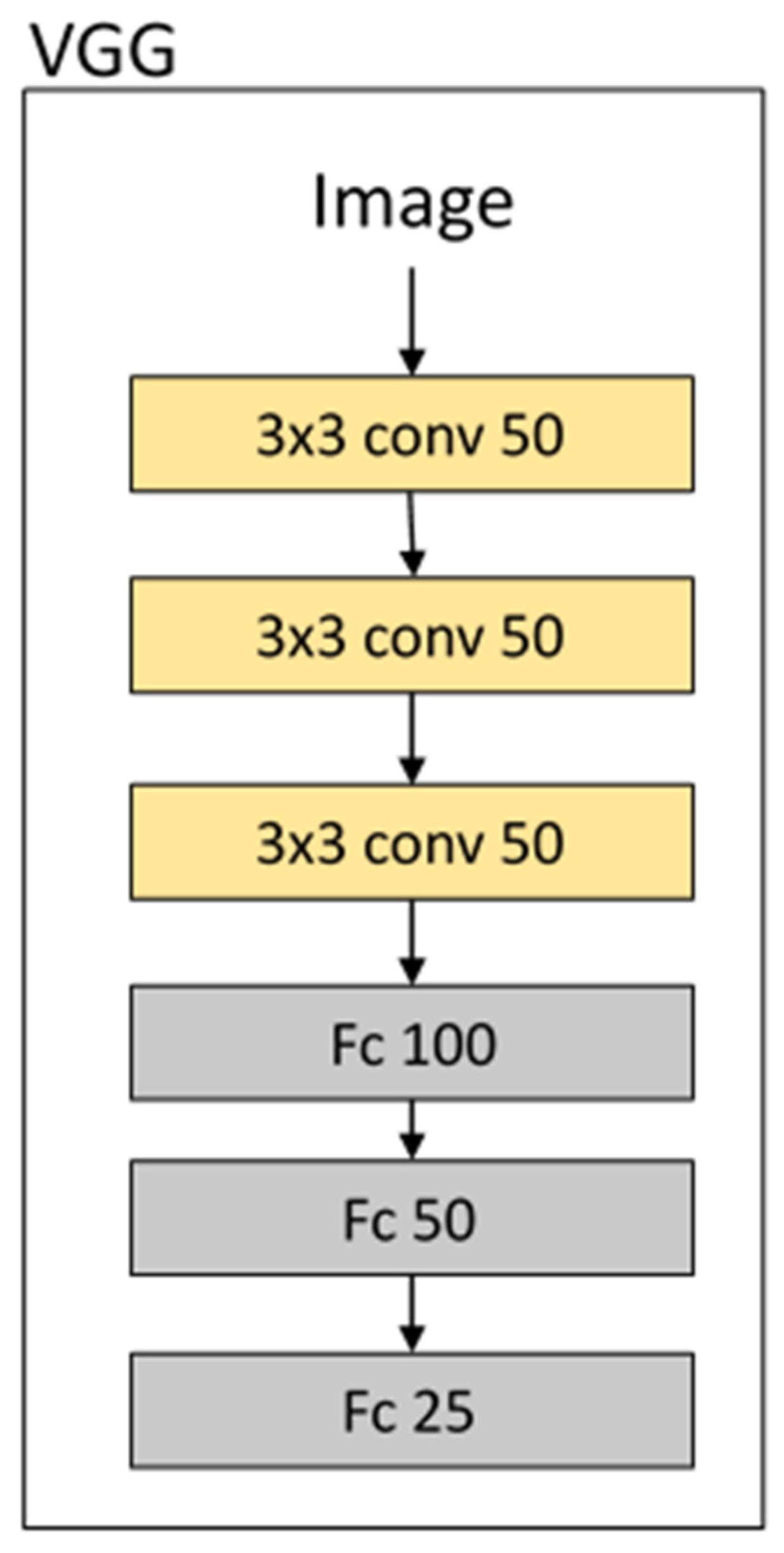
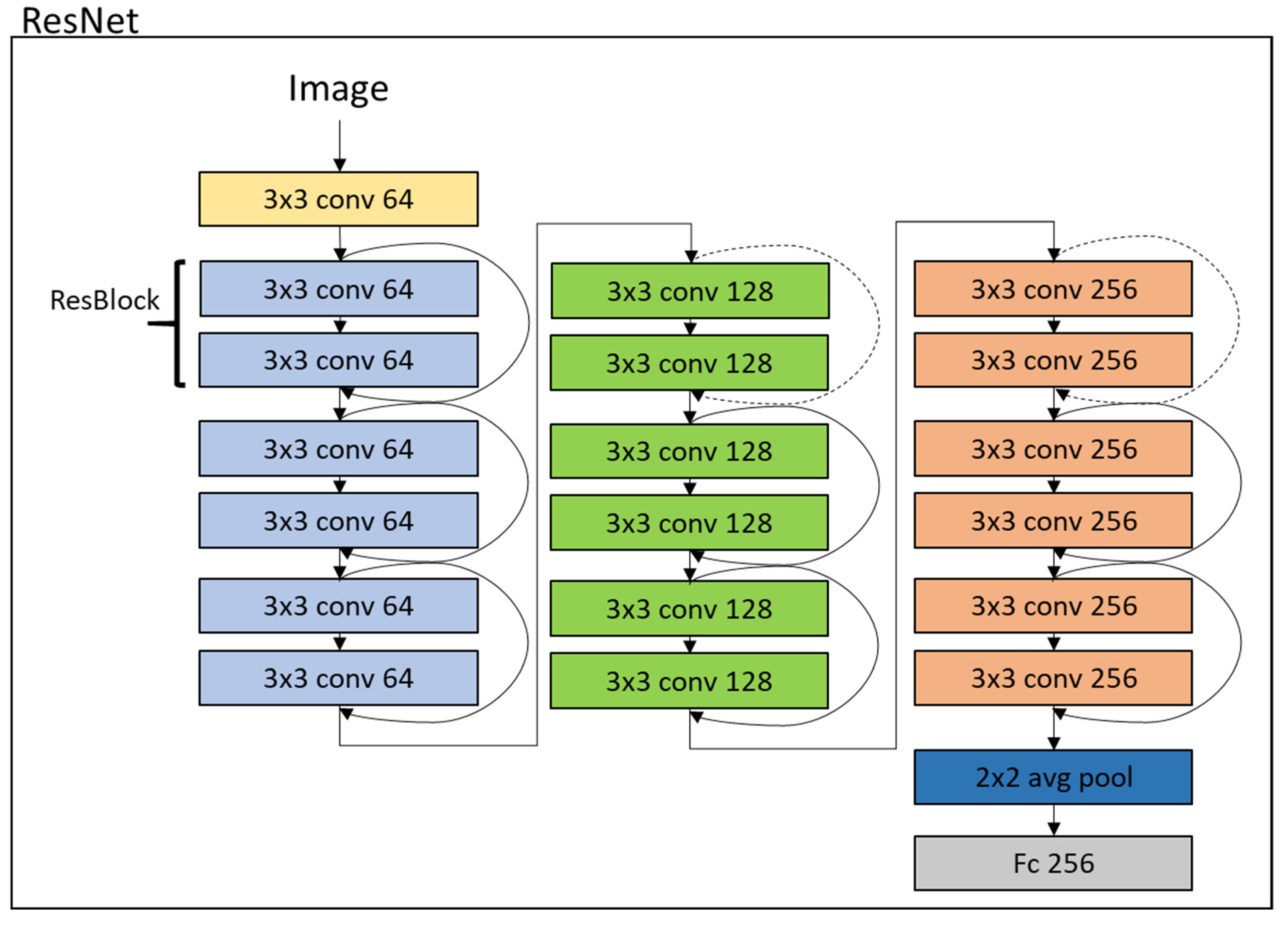
In the training of SLALOM-CT, we firstly carried out a systematic model selection, comparing different pixel-based and image-based machine learning algorithms. The analysis focused on two specific problems: the detection of the snowfall rate areas (SD module) and the estimate of the snow water path (SPE module). The results of this intercomparison paved the way for a number of considerations. First, the performances of NNs are systematically better than those of decision tree algorithms (random forests and gradient boosting) for both SD and SWP estimation problems. This result is not necessarily generalizable to other radiometers, as it is strictly related to the specific characteristics (in terms of size and signal-to-noise ratio) of the dataset used and to the channels and viewing geometry of the radiometer considered. However, for ATMS snowfall retrieval, NNs seem to be more promising than ensemble trees. Therefore, the NN approach was chosen for the SCD and SR modules, with only a limited testing of different approaches (not shown here). A second result arises from the comparison of pixel-based and image-based neural networks. The convolutional neural networks that were chosen for this study take as input a 7 × 7-pixel image for each input variable (i.e., 16 BTs and 18 ancillary variables), and produce the output (for the estimate or classification) in the central pixel of the image. These architectures are therefore similar to the pixel-based networks and allow a direct comparison of the pixel- and image-based approaches. In particular, the main differences between the pixel- and image-based NN results should come from the contribution that the pixels surrounding the central pixel can provide to the solution of the given problem. In the framework of precipitation retrievals from PMW sensors, the use of information from surrounding pixels has already been explored by some authors. The convolutional NN approach to this problem is, however, completely different, as the optimization of convolutional weights that are trained to recognize and extract specific features from the BT image is far more sophisticated and promising.

For our applications, some examples of features that we can extract from BTs are gradients and convex or concave shapes, together with combinations of these (including their variability with the channel frequency). Another point that is important to stress is that the NNs tested differ in their depth or complexity. One main result in the model selection is that, in our case, there is a limit to the complexity of the model that can successfully solve a given problem, and this limit is set by the size of the training dataset and by the noise level associated with the variables in it. In our case, the shallow pixel-based network was the most efficient model for the SPE problem, while the relatively simple VGG model was the most suitable for the SD problem. Evidently, in this second case, the contribution provided by the surrounding pixels was substantial. Moreover, ResNet (deeper and more complex than VGG) gave a worse performance than the simpler networks due to the limited size of the dataset. However, the fact that all results from NNs are quite similar supports the hypothesis that all the algorithms trained reached the maximum level of accuracy, strictly related to the noise level.

The SLALOM-CT algorithm produced very good results, which is satisfying given the complexity of the remote sensing of snow. The quality of these results was also highlighted by the comparison with a reference algorithm (the NASA GPM official PMW precipitation retrieval algorithm, GPROF). SLALOM-CT was compared with GPROF using CPR as a reference, showing smaller errors and far better detection capability. This was confirmed also by comparing SLALOM-CT with GPROF over snow-covered surfaces, where GPROF uses, as precipitation information in the a priori database, the MRMS precipitation rate. With regard to this comparison and in particular to the results of GPROF, it should be mentioned that in some studies on the quality assessment of GPROF-GMI V05 snowfall rate estimates, some issues were also noted. In an assessment carried out over southern Finland, a very low ability to detect shallow snowfall events was found for GPROF-GMI [104]. Moreover, in a study on intense lake-effect snow events over the lower US Great Lakes region, Milani et al. [105] found that GPROF-GMI misses and/or underestimates intense (and shallow) lake-effect snowfall. Skofronick-Jackson et al. [2] also provided additional evidence of the GPROF-GMI shallow convective snowfall detection limitations. The results of GPROF-GMI are not directly comparable to those of this work, because of the many differences between the two radiometers. Moreover, a fair comparison of SLALOM-CT and GPROF-ATMS should be based on a reference dataset not used in the training or as a priori information in either of the two algorithms. However, the Mroz et al. study [68], where an extensive validation of SLALOM and GPROF (for GMI) was carried out using the MRMS product, showed poorer results for GPROF, which evidently were not due to the selection of the reference dataset. The different results found for SLALOM-CT and GPROF can be attributed to the characteristics of the two algorithms, namely the input variables used (GPROF ignores the ATMS 50–60 GHz channels and uses a daily snow-cover/sea ice map and fewer model-derived variables) and the retrieval technique (Bayesian vs. machine learning). Complex machine learning algorithms (such as those of SLALOM-CT) are able to discriminate more efficiently between the subtle and complex signal of snowfall and the variable and misleading contribution due to the background surface, environmental conditions, and supercooled liquid water within the cloud. Moreover, recently, a set of snowfall detection algorithms over ocean, sea ice, and coast, based on logistic regression for ATMS was developed, using CPR as a reference [106]. This algorithm has good detection capabilities (i.e., a POD and FAR equal to 79% and 35%, respectively, over ocean and slightly worse values over sea-ice and coastal areas); however, SLALOM-CT shows better performance over both ocean and coast (see Table 8), and also over sea ice (aggregated statistics for the PESCA sea ice surfaces were 82%, 20%, and 63% for POD, FAR, and HSS, respectively). These results confirm the ability of the machine-learning-based approaches to learn and generalize the relations between the ATMS channels and the CPR snowfall rates. However, in a recent study by Adhikari et al. [37], the RF-MHS algorithm was trained using random forests for detecting and estimating snowfall rates from MHS BTs using CPR as a reference. The performance of RF-MHS was worse than SLALOM-CT, in both detection (POD of 0.55 and FAR of 0.45) and snowfall estimate statistics (RMSE of 0.23–0.40 mm/h, correlation of 0.23–0.57). The disagreement in the results was probably related more to the differences in the input used (MHS carries only five channels at high frequency, and the authors use a very limited number of environmental variables) than to the machine learning approach chosen. In fact, even comparing the ATMS RF snowfall detection statistics (see Table 5) with those of RF-MHS, a large disagreement is still present.

In a recent study by Takbiri et al. [97], it was shown that the liquid water content of clouds and the snow-cover depth impact the observed BT signals in high-frequency channels and can mask the relatively small signal due to snowfall. In particular, the emission due to liquid water tends to enhance the BTs, while a deeper snow cover tends to lower the surface emissivity, and these effects tend to mask the scattering signal produced by snowflakes. The authors define some conditions in terms of snow depth and LWP (i.e., a snow depth greater than 200 kg m⁻² SWE and cloud LWP lower than 100–150 g m⁻²) as a blind zone, where the PMW cannot detect or estimate snowfall. In our study, we observed that the presence of liquid water has a strong impact on the detection of snowfall (increasing the rate of false alarms), while we did not notice any impact from snow-cover depth. This may be due to the categorization of snow cover at the time of the overpass that was performed by the PESCA algorithm and used as input in SLALOM-CT. Another explanation could be that our algorithm can better discriminate the signal produced by snowfall from those due to surface-related or atmospheric effects, compared with the analysis carried out in [97], where the analysis focused on GMI high-frequency window channels only (89 and 166 GHz). Moreover, our analysis showed that SLALOM-CT error statistics were almost independent of the surface category, which strongly affects the ground emissivity, as shown in Camplani et al. 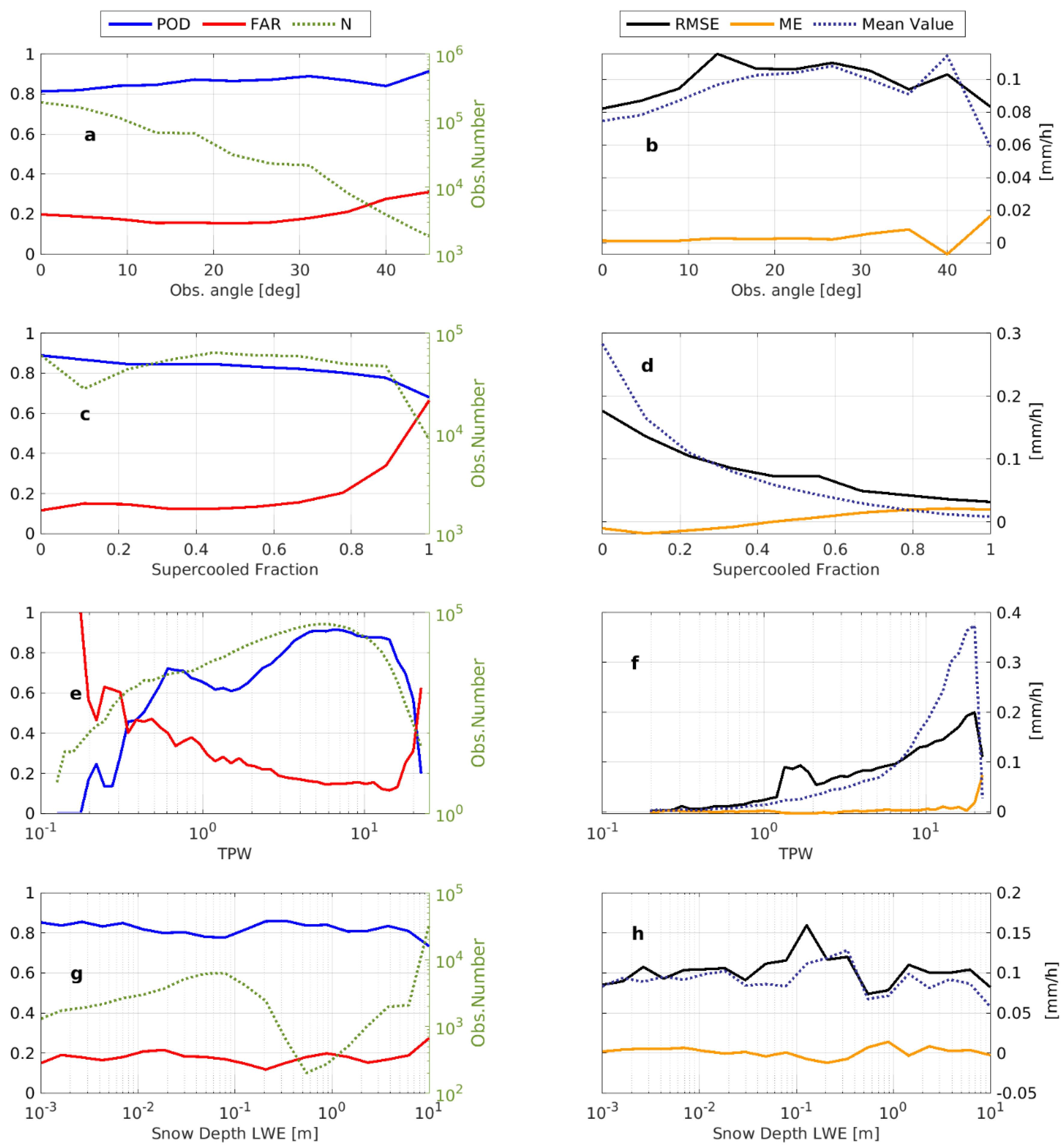[93]. We can assume that the NN modules within SLALOM-CT can exploit the categorization of the surface and use this information to mitigate the issues deriving from the extremely variable emissivity of the cold surfaces (snow cover and sea ice). It should also be highlighted that the SLALOM-CT performance is not affected by the observation angle, even though the ATMS view geometry, as a cross-track radiometer, is considerably more complex than conical scanners. The viewing geometry affects both the geometrical thickness of the observed atmosphere and the emission spectrum of the ground, with significant effects also in the polarization of the signal emitted by the surface. The fact that SLALOM-CT error statistics seem to be independent of the viewing geometry confirms that, during the training phase, the observation angle (which is one of the SLALOM-CT inputs) was optimally exploited.

6. Conclusions

A new ML-based algorithm named SLALOM-CT (Snow retrievaL ALgorithm fOr gpM–Cross Track) was designed and developed using, for the training phase, coincident ATMS and CPR observations. The algorithm is composed of independent modules for the detection of snowfall (SD) and supercooled droplets (SCD), for the estimate of snow water path (SPE) and of the snowfall rate (SRE). Each module was selected from several optimized machine learning algorithms. The techniques that were compared to identify the best performance were decision trees (random forests and gradient boosting) and NNs. In particular, both shallow (pixel-based) and convolutional (image-based) networks were analyzed, considering different levels of depth and complexity. The final SLALOM-CT algorithm showed very good performance in the detection and estimation of snowfall rates, especially when compared with state-of-the-art satellite products for the estimation of precipitation (GPROF–ATMS). Particularly relevant is the substantial homogeneity of the algorithm performance considering different radiometer viewing angles, snow-cover depths, and surface categories.

This work is part of the development of precipitation retrieval algorithms for the new EPS-SG satellites. In particular, the similarities between ATMS and MWS, which will be on board the EPS-SG-A series of satellites, make SLALOM-CT the precursor of the day-1 MWS algorithm for snowfall retrieval. Further work related to this study will be to test the potential of the convolutional neural networks for other radiometers, including conically scanning radiometers and GMI in particular. In this context, some techniques developed for transfer learning seem very promising. Moreover, the SLALOM-CT capabilities should be verified with independent ground-based references such as radar networks and snow pits.

References

1. Cordisco, E.; Prigent, C.; Aires, F. Snow characterization at a global scale passive microwave satelite observations. J. Geophys. Res. Atmos. 2006, 111, D19102. [Google Scholar] [CrossRef] [Green Version]
2. Skofronick-Jackson, G.; Kulie, M.; Milani, L.; Munchak, S.J.; Wood, N.; Levizzani, V. Satellite Estimation of Falling Snow: A Global Precipitation Measurement (GPM) Core Observatory Perspective. J. Appl. Meteorol. Climatol. 2019, 58, 1429–1448. [Google Scholar] [CrossRef] [PubMed]
3. Liu, G. Radar Snowfall Measurement. In Advances in Global Change Research; Springer: Cham, Switzerland, 2020; Volume 67. [Google Scholar]
4. Vahedizade, S.; Ebtehaj, A.; You, Y.; Ringerud, S.E.; Turk, F.J. Passive Microwave Signatures and Retrieval of High-Latitude Snowfall Over Open Oceans and Sea Ice: Insights from Coincidences of GPM and CloudSat Satellites. IEEE Trans. Geosci. Remote Sens. 2021, 60, 4300913. [Google Scholar] [CrossRef]
5. Behrangi, A.; Christensen, M.; Richardson, M.; Lebsock, M.; Stephens, G.; Huffman, G.; Bolvin, D.; Adler, R.F.; Gardner, A.; Lambrigtsen, B.; et al. Status of high-latitude precipitation estimates from observations and reanalyses. J. Geophys. Res. Atmos. 2016, 121, 4468–4486. [Google Scholar] [CrossRef] [PubMed]
6. Field, P.R.; Heymsfield, A.J. Importance of snow to global precipitation. Geophys. Res. Lett. 2015, 42, 9512–9520. [Google Scholar] [CrossRef] [Green Version]
7. Liu, G.; Curry, J.A. Precipitation characteristics in Greenland-Iceland-Norwegian Seas determined by using satellite microwave data. J. Geophys. Res. Earth Surf. 1997, 102, 13987–13997. [Google Scholar] [CrossRef]
8. Levizzani, V.; Laviola, S.; Cattani, E. Detection and Measurement of Snowfall from Space. Remote Sens. 2011, 3, 145–166. [Google Scholar] [CrossRef] [Green Version]
9. Kidd, C.; Becker, A.; Huffman, G.; Muller, C.L.; Joe, P.; Skofronick-Jackson, G.; Kirschbaum, D. So, How Much of the Earth’s Surface Is Covered by Rain Gauges? Bull. Am. Meteorol. Soc. 2017, 98, 69–78. [Google Scholar] [CrossRef]
10. Behrangi, A.; Gardner, A.; Reager, J.T.; Fisher, J.B.; Yang, D.; Huffman, G.J.; Adler, R.F. Using GRACE to Estitmate Snowfall Accumulation and Assess Gauge Undercatch Corrections in High Latitudes. J. Clim. 2018, 31, 8689–8704. [Google Scholar] [CrossRef]
11. Panahi, M.; Behrangi, A. Comparative Analysis of Snowfall Accumulation and Gauge Undercatch Correction Factors from Diverse Data Sets: In Situ, Satellite, and Reanalysis. Asia-Pac. J. Atmos. Sci. 2019, 56, 615–628. [Google Scholar] [CrossRef]
12. Kongoli, C.; Meng, H.; Dong, J.; Ferraro, R. A snowfall detection algorithm over land utilizing high-frequency passive microwave measurements-Application to ATMS. J. Geophys. Res. Atmos. 2015, 120, 1918–1932. [Google Scholar] [CrossRef]
13. Kongoli, C.; Meng, H.; Dong, J.; Ferraro, R. A hybrid snowfall detection method from satellite passive microwave measurements and global forecast weather models. Q. J. R. Meteorol. Soc. 2018, 144, 120–132. [Google Scholar] [CrossRef] [Green Version]
14. Kongoli, C.; Pellegrino, P.; Ferraro, R.; Grody, N.C.; Meng, H. A new snowfall detection algorithm over land using measurements from the Advanced Microwave Sounding Unit (AMSU). Geophys. Res. Lett. 2003, 30. [Google Scholar] [CrossRef]
15. Rysman, J.-F.; Panegrossi, G.; Sanò, P.; Marra, A.C.; Dietrich, S.; Milani, L.; Kulie, M.S. SLALOM: An All-Surface Snow Water Path Retrieval Algorithm for the GPM Microwave Imager. Remote Sens. 2018, 10, 1278. [Google Scholar] [CrossRef] [Green Version]
16. Skofronick-Jackson, G.; Hudak, D.; Petersen, W.; Nesbitt, S.; Chandrasekar, V.; Durden, S.; Gleicher, K.J.; Huang, G.-J.; Joe, P.; Kollias, P.; et al. Global Precipitation Measurement Cold Season Precipitation Experiment (GCPEX): For Measurement’s Sake, Let It Snow. Bull. Am. Meteorol. Soc. 2015, 96, 1719–1741. [Google Scholar] [CrossRef]
17. Skofronick-Jackson, G.M.; Johnson, B.T.; Munchak, S.J. Detection Thresholds of Falling Snow From Satellite-Borne Active and Passive Sensors. IEEE Trans. Geosci. Remote Sens. 2013, 51, 4177–4189. [Google Scholar] [CrossRef] [Green Version]
18. Noh, Y.-J.; Liu, G.; Seo, E.-K.; Wang, J.R.; Aonashi, K. Development of a snowfall retrieval algorithm at high microwave frequencies. J. Geophys. Res. Atmos. 2006, 111, D22216. [Google Scholar] [CrossRef]
19. Grecu, M.; Olson, W.S. Precipitating Snow Retrievals from Combined Airborne Cloud Radar and Millimeter-Wave Radiometer Observations. J. Appl. Meteorol. Climatol. 2008, 47, 1634–1650. [Google Scholar] [CrossRef]
20. Munchak, S.J.; Skofronick-Jackson, G. Evaluation of precipitation detection over various surfaces from passive microwave imagers and sounders. Atmos. Res. 2013, 131, 81–94. [Google Scholar] [CrossRef]
21. Liu, G.; Seo, E.-K. Detecting snowfall over land by satellite high-frequency microwave observations: The lack of scattering signature and a statistical approach. J. Geophys. Res. Atmos. 2013, 118, 1376–1387. [Google Scholar] [CrossRef]
22. Ebtehaj, A.M.; Kummerow, C.D. Microwave retrievals of terrestrial precipitation over snow-covered surfaces: A lesson from the GPM satellite. Geophys. Res. Lett. 2017, 44, 6154–6162. [Google Scholar] [CrossRef]
23. You, Y.; Wang, N.-Y.; Ferraro, R.; Rudlosky, S. Quantifying the Snowfall Detection Performance of the GPM Microwave Imager Channels over Land. J. Hydrometeorol. 2017, 18, 729–751. [Google Scholar] [CrossRef]
24. Kulie, M.S.; Bennartz, R.; Greenwald, T.J.; Chen, Y.; Weng, F. Uncertainties in Microwave Properties of Frozen Precipitation: Implications for Remote Sensing and Data Assimilation. J. Atmos. Sci. 2010, 67, 3471–3487. [Google Scholar] [CrossRef] [Green Version]
25. Skofronick-Jackson, G.; Johnson, B.T. Surface and atmospheric contributions to passive microwave brightness temperatures for falling snow events. J. Geophys. Res. Earth Surf. 2011, 116. [Google Scholar] [CrossRef]
26. Eriksson, P.; Jamali, M.; Mendrok, J.; Buehler, S.A. On the microwave optical properties of randomly oriented ice hydrometeors. Atmos. Meas. Tech. 2015, 8, 1913–1933. [Google Scholar] [CrossRef] [Green Version]
27. Bennartz, R.; Bauer, P. Sensitivity of microwave radiances at 85-183 GHz to precipitating ice particles. Radio Sci. 2003, 38. [Google Scholar] [CrossRef]
28. Di Michele, S.; Bauer, P. Passive microwave radiometer channel selection based on cloud and precipitation information content. Q. J. R. Meteorol. Soc. 2006, 132, 1299–1323. [Google Scholar] [CrossRef]
29. Edel, L.; Rysman, J.-F.; Claud, C.; Palerme, C.; Genthon, C. Potential of Passive Microwave around 183 GHz for Snowfall Detection in the Arctic. Remote Sens. 2019, 11, 2200. [Google Scholar] [CrossRef] [Green Version]
30. Panegrossi, G.; Rysman, J.-F.; Casella, D.; Marra, A.C.; Sanò, P.; Kulie, M.S. CloudSat-Based Assessment of GPM Microwave Imager Snowfall Observation Capabilities. Remote Sens. 2017, 9, 1263. [Google Scholar] [CrossRef] [Green Version]
31. Kongoli, C.; Meng, H.; Dong, J.; Ferraro, R. Ground-based Assessment of Snowfall Detection over Land Using Polarimetric High Frequency Microwave Measurements. Remote Sens. 2020, 12, 3441. [Google Scholar] [CrossRef]
32. Chen, S.; Hong, Y.; Kulie, M.; Behrangi, A.; Stepanian, P.M.; Cao, Q.; You, Y.; Zhang, J.; Hu, J.; Zhang, X. Comparison of snowfall estimates from the NASA CloudSat Cloud Profiling Radar and NOAA/NSSL Multi-Radar Multi-Sensor System. J. Hydrol. 2016, 541, 862–872. [Google Scholar] [CrossRef]
33. Kulie, M.S.; Milani, L.; Wood, N.; Tushaus, S.A.; Bennartz, R.; L’Ecuyer, T. A Shallow Cumuliform Snowfall Census Using Spaceborne Radar. J. Hydrometeorol. 2016, 17, 1261–1279. [Google Scholar] [CrossRef]
34. Kulie, M.S.; Milani, L.; Wood, N.B.; L’Ecuyer, T.S. Global Snowfall Detection and Measurement. In Advances in Global Change Research; Springer: Cham, Switzerland, 2020; Volume 69. [Google Scholar]
35. Hamada, A.; Iguchi, T.; Takayabu, Y.N. Snowfall Detection by Spaceborne Radars. In Advances in Global Change Research; Springer: Cham, Switzerland, 2020; Volume 69. [Google Scholar]
36. Casella, D.; Panegrossi, G.; Sanò, P.; Marra, A.C.; Dietrich, S.; Johnson, B.T.; Kulie, M.S. Evaluation of the GPM-DPR snowfall detection capability: Comparison with CloudSat-CPR. Atmos. Res. 2017, 197, 64–75. [Google Scholar] [CrossRef]
37. Adhikari, A.; Ehsani, M.R.; Song, Y.; Behrangi, A. Comparative Assessment of Snowfall Retrieval from Microwave Humidity Sounders Using Machine Learning Methods. Earth Space Sci. 2020, 7, e2020EA001357. [Google Scholar] [CrossRef]
38. Takbiri, Z.; Ebtehaj, A.; Foufoula-Georgiou, E.; Kirstetter, P.-E.; Turk, F.J. A Prognostic Nested k-Nearest Approach for Microwave Precipitation Phase Detection over Snow Cover. J. Hydrometeorol. 2019, 20, 251–274. [Google Scholar] [CrossRef]
39. Johnson, B.T.; Olson, W.S.; Skofronick-Jackson, G. The microwave properties of simulated melting precipitation particles: Sensitivity to initial melting. Atmos. Meas. Tech. 2016, 9, 9–21. [Google Scholar] [CrossRef] [Green Version]
40. Wang, Y.; Liu, G.; Seo, E.-K.; Fu, Y. Liquid water in snowing clouds: Implications for satellite remote sensing of snowfall. Atmos. Res. 2012, 131, 60–72. [Google Scholar] [CrossRef]
41. Liou, Y.-A.; Tzeng, Y.; Chen, K. A neural-network approach to radiometric sensing of land-surface parameters. IEEE Trans. Geosci. Remote Sens. 1999, 37, 2718–2724. [Google Scholar] [CrossRef]
42. Aires, F.; Prigent, C.; Rossow, W.B.; Rothstein, M. A new neural network approach including first guess for retrieval of atmospheric water vapor, cloud liquid water path, surface temperature, and emissivities over land from satellite microwave observations. J. Geophys. Res. Earth Surf. 2001, 106, 14887–14907. [Google Scholar] [CrossRef]
43. Boukabara, S.-A.; Krasnopolsky, V.; Penny, S.G.; Stewart, J.Q.; McGovern, A.; Hall, D.; Hoeve, J.E.T.; Hickey, J.; Huang, H.-L.A.; Williams, J.K.; et al. Outlook for Exploiting Artificial Intelligence in the Earth and Environmental Sciences. Bull. Am. Meteorol. Soc. 2021, 102, E1016–E1032. [Google Scholar] [CrossRef]
44. Blackwell, W.J.; Chen, F.W. Neural Network Applications in High-Resolution Atmospheric Remote Sensing. Linc. Lab. J. 2005, 15, 299. [Google Scholar]
45. Surussavadee, C.; Staelin, D.H. Global Millimeter-Wave Precipitation Retrievals Trained With a Cloud-Resolving Numerical Weather Prediction Model, Part I: Retrieval Design. IEEE Trans. Geosci. Remote Sens. 2007, 46, 99–108. [Google Scholar] [CrossRef]
46. Mahesh, C.; Prakash, S.; Sathiyamoorthy, V.; Gairola, R. Artificial neural network based microwave precipitation estimation using scattering index and polarization corrected temperature. Atmos. Res. 2011, 102, 358–364. [Google Scholar] [CrossRef]
47. Sanò, P.; Panegrossi, G.; Casella, D.; Marra, A.C.; Di Paola, F.; Dietrich, S. The new Passive microwave Neural network Precipitation Retrieval (PNPR) algorithm for the cross-track scanning ATMS radiometer: Description and verification study over Europe and Africa using GPM and TRMM spaceborne radars. Atmos. Meas. Tech. 2016, 9, 5441–5460. [Google Scholar] [CrossRef] [Green Version]
48. Sanò, P.; Panegrossi, G.; Casella, D.; Marra, A.C.; D’Adderio, L.P.; Rysman, J.F.; Dietrich, S. The Passive Microwave Neural Network Precipitation Retrieval (PNPR) Algorithm for the CONICAL Scanning Global Microwave Imager (GMI) Radiometer. Remote Sens. 2018, 10, 1122. [Google Scholar] [CrossRef] [Green Version]
49. Ghorbanzadeh, O.; Blaschke, T.; Gholamnia, K.; Meena, S.R.; Tiede, D.; Aryal, J. Evaluation of Different Machine Learning Methods and Deep-Learning Convolutional Neural Networks for Landslide Detection. Remote Sens. 2019, 11, 196. [Google Scholar] [CrossRef] [Green Version]
50. Prakash, N.; Manconi, A.; Loew, S. Mapping Landslides on EO Data: Performance of Deep Learning Models vs. Traditional Machine Learning Models. Remote Sens. 2020, 12, 346. [Google Scholar] [CrossRef] [Green Version]
51. Boukabara, S.-A.; Krasnopolsky, V.; Stewart, J.Q.; Maddy, E.S.; Shahroudi, N.; Hoffman, R.N. Leveraging Modern Artificial Intelligence for Remote Sensing and NWP: Benefits and Challenges. Bull. Am. Meteorol. Soc. 2019, 100, ES473–ES491. [Google Scholar] [CrossRef]
52. Tedesco, M.; Pulliainen, J.; Takala, M.; Hallikainen, M.; Pampaloni, P. Artificial neural network-based techniques for the retrieval of SWE and snow depth from SSM/I data. Remote Sens. Environ. 2004, 90, 76–85. [Google Scholar] [CrossRef]
53. Tabari, H.; Marofi, S.; Abyaneh, H.Z.; Sharifi, M.R. Comparison of artificial neural network and combined models in estimating spatial distribution of snow depth and snow water equivalent in Samsami basin of Iran. Neural Comput. Appl. 2009, 19, 625–635. [Google Scholar] [CrossRef]
54. Rysman, J.; Panegrossi, G.; Sanò, P.; Marra, A.C.; Dietrich, S.; Milani, L.; Kulie, M.S.; Casella, D.; Camplani, A.; Claud, C.; et al. Retrieving Surface Snowfall with the GPM Microwave Imager: A New Module for the SLALOM Algorithm. Geophys. Res. Lett. 2019, 46, 13593–13601. [Google Scholar] [CrossRef]
55. Tsai, Y.-L.S.; Dietz, A.; Oppelt, N.; Kuenzer, C. Wet and Dry Snow Detection Using Sentinel-1 SAR Data for Mountainous Areas with a Machine Learning Technique. Remote Sens. 2019, 11, 895. [Google Scholar] [CrossRef] [Green Version]
56. Hicks, A.; Notaroš, B.M. Method for Classification of Snowflakes Based on Images by a Multi-Angle Snowflake Camera Using Convolutional Neural Networks. J. Atmos. Ocean. Technol. 2019, 36, 2267–2282. [Google Scholar] [CrossRef]
57. Roebber, P.J.; Butt, M.R.; Reinke, S.J.; Grafenauer, T.J. Real-Time Forecasting of Snowfall Using a Neural Network. Weather Forecast. 2007, 22, 676–684. [Google Scholar] [CrossRef]
58. Liu, J.; Zhang, Y.; Cheng, X.; Hu, Y. Retrieval of Snow Depth over Arctic Sea Ice Using a Deep Neural Network. Remote Sens. 2019, 11, 2864. [Google Scholar] [CrossRef] [Green Version]
59. Casella, D.; Amaral, L.M.C.D.; Dietrich, S.; Marra, A.C.; Sano, P.; Panegrossi, G. The Cloud Dynamics and Radiation Database Algorithm for AMSR2: Exploitation of the GPM Observational Dataset for Operational Applications. IEEE J. Sel. Top. Appl. Earth Obs. Remote Sens. 2017, 10, 3985–4001. [Google Scholar] [CrossRef]
60. Panegrossi, G.; Dietrich, S.; Marzano, F.S.; Mugnai, A.; Smith, E.A.; Xiang, X.; Tripoli, G.J.; Wang, P.K.; Baptista, J.P.V.P. Use of Cloud Model Microphysics for Passive Microwave-Based Precipitation Retrieval: Significance of Consistency between Model and Measurement Manifolds. J. Atmos. Sci. 1998, 55, 1644–1673. [Google Scholar] [CrossRef]
61. Di Michele, S.; Tassa, A.; Mugnai, A.; Marzano, F.; Bauer, P.; Baptista, J. Bayesian algorithm for microwave-based precipitation retrieval: Description and application to TMI measurements over ocean. IEEE Trans. Geosci. Remote Sens. 2005, 43, 778–791. [Google Scholar] [CrossRef]
62. Kummerow, C.; Hong, Y.; Olson, W.S.; Yang, S.; Adler, R.F.; Mccollum, J.; Ferraro, R.; Petty, G.; Shin, D.-B.; Wilheit, T.T. The Evolution of the Goddard Profiling Algorithm (GPROF) for Rainfall Estimation from Passive Microwave Sensors. J. Appl. Meteorol. 2001, 40, 1801–1820. [Google Scholar] [CrossRef]
63. Casella, D.; Panegrossi, G.; Sanò, P.; Dietrich, S.; Mugnai, A.; Smith, E.A.; Tripoli, G.J.; Formenton, M.; Di Paola, F.; Leung, W.-Y.H.; et al. Transitioning From CRD to CDRD in Bayesian Retrieval of Rainfall from Satellite Passive Microwave Measurements: Part 2. Overcoming Database Profile Selection Ambiguity by Consideration of Meteorological Control on Microphysics. IEEE Trans. Geosci. Remote Sens. 2013, 51, 4650–4671. [Google Scholar] [CrossRef]
64. Sano, P.; Casella, D.; Mugnai, A.; Schiavon, G.; Smith, E.A.; Tripoli, G.J. Transitioning from CRD to CDRD in bayesian retrieval of rainfall from satellite passive microwave measurements: Part 1. Algorithm description and testing. IEEE Trans. Geosci. Remote Sens. 2013, 51, 4119–4143. [Google Scholar] [CrossRef]
65. Sanò, P.; Casella, D.; Panegrossi, G.; Marra, A.C.; Petracca, M.; Dietrich, S. The Passive Microwave Neural Network Precipitation Retrieval (PNPR) for the Cross-track Scanning ATMS Radiometer. In Proceedings of the 2015 EUMETSAT Meteorological Satellite Conference, Toulouse, France, 21–25 September 2015. [Google Scholar]
66. Kuo, K.-S.; Olson, W.S.; Johnson, B.T.; Grecu, M.; Tian, L.; Clune, T.L.; van Aartsen, B.H.; Heymsfield, A.J.; Liao, L.; Meneghini, R. The Microwave Radiative Properties of Falling Snow Derived from Nonspherical Ice Particle Models. Part I: An Extensive Database of Simulated Pristine Crystals and Aggregate Particles, and Their Scattering Properties. J. Appl. Meteorol. Climatol. 2016, 55, 691–708. [Google Scholar] [CrossRef]
67. Milani, L.; Wood, N. Biases in CloudSat Falling Snow Estimates Resulting from Daylight-Only Operations. Remote Sens. 2021, 13, 2041. [Google Scholar] [CrossRef]
68. Mroz, K.; Montopoli, M.; Battaglia, A.; Panegrossi, G.; Kirstetter, P.; Baldini, L. Cross-validation of active and passive microwave snowfall products over the continental United States. J. Hydrometeorol. 2021, 22, 1297–1315. [Google Scholar] [CrossRef]
69. Battaglia, A.; Panegrossi, G. What Can We Learn from the CloudSat Radiometric Mode Observations of Snowfall over the Ice-Free Ocean? Remote Sens. 2020, 12, 3285. [Google Scholar] [CrossRef]
70. Boukabara, S.-A.; Garrett, K.; Grassotti, C.; Iturbide-Sanchez, F.; Chen, W.; Jiang, Z.; Clough, S.A.; Zhan, X.; Liang, P.; Liu, Q.; et al. A physical approach for a simultaneous retrieval of sounding, surface, hydrometeor, and cryospheric parameters from SNPP/ATMS. J. Geophys. Res. Atmos. 2013, 118, 12–600. [Google Scholar] [CrossRef]
71. Weng, F.; Zou, X.; Wang, X.; Yang, S.; Goldberg, M.D. Introduction to Suomi national polar-orbiting partnership advanced technology microwave sounder for numerical weather prediction and tropical cyclone applications. J. Geophys. Res. Atmos. 2012, 117, D19112. [Google Scholar] [CrossRef]
72. Goldberg, M.D.; Kilcoyne, H.; Cikanek, H.; Mehta, A. Joint Polar Satellite System: The United States next generation civilian polar-orbiting environmental satellite system. J. Geophys. Res. Atmos. 2013, 118, 13463–13475. [Google Scholar] [CrossRef]
73. Zou, X.; Weng, F.; Zhang, B.; Lin, L.; Qin, Z.; Tallapragada, V. Impacts of assimilation of ATMS data in HWRF on track and intensity forecasts of 2012 four landfall hurricanes. J. Geophys. Res. Atmos. 2013, 118, 11558–11576. [Google Scholar] [CrossRef]
74. Wood, N.B.; L’Ecuyer, T.S.; Heymsfield, A.J.; Stephens, G.L.; Hudak, D.R.; Rodriguez, P. Estimating snow microphysical properties using collocated multisensor observations. J. Geophys. Res. Atmos. 2014, 119, 8941–8961. [Google Scholar] [CrossRef]
75. Rodgers, C.D. Inverse Methods for Atmospheric Sounding: Theory and Practice, Series on Atmospheric, Oceanic and Planetary Physics; World Scientific: Singapore, 2000; Volume 2. [Google Scholar]
76. Ceccaldi, M.; Delanoë, J.; Hogan, R.J.; Pounder, N.L.; Protat, A.; Pelon, J. From CloudSat-CALIPSO to EarthCare: Evolution of the DARDAR cloud classification and its comparison to airborne radar-lidar observations. J. Geophys. Res. Atmos. 2013, 118, 7962–7981. [Google Scholar] [CrossRef]
77. Kummerow, C.D.; Giglio, L. A Passive Microwave Technique for Estimating Rainfall and Vertical Structure Information from Space. Part I: Algorithm Description. J. Appl. Meteorol. 1994, 33, 3–18. [Google Scholar] [CrossRef]
78. Kidd, C.; Matsui, T.; Chern, J.; Mohr, K.; Kummerow, C.; Randel, D. Global Precipitation Estimates from Cross-Track Passive Microwave Observations Using a Physically Based Retrieval Scheme. J. Hydrometeorol. 2015, 17, 383–400. [Google Scholar] [CrossRef] [Green Version]
79. Kummerow, C.D.; Randel, D.L.; Kulie, M.; Wang, N.-Y.; Ferraro, R.; Munchak, S.J.; Petkovic, V. The Evolution of the Goddard Profiling Algorithm to a Fully Parametric Scheme. J. Atmos. Ocean. Technol. 2015, 32, 2265–2280. [Google Scholar] [CrossRef]
80. Randel, D.L.; Kummerow, C.D.; Ringerud, S. The Goddard Profiling (GPROF) Precipitation Retrieval Algorithm. In Advances in Global Change Research; Springer: Cham, Switzerland, 2020; Volume 67. [Google Scholar]
81. Breiman, L. Bagging predictors. Mach. Learn. 1996, 24, 123–140. [Google Scholar] [CrossRef] [Green Version]
82. Breiman, L. Random forests. Mach. Learn. 2001, 45, 5–32. [Google Scholar] [CrossRef] [Green Version]
83. Tapiador, F.J.; Kidd, C.; Hsu, K.-L.; Marzano, F. Neural networks in satellite rainfall estimation. Meteorol. Appl. 1999, 11, 83–91. [Google Scholar] [CrossRef] [Green Version]
84. Haykin, S. Neural networks: A comprehensive foundation by Simon Haykin. Knowl. Eng. Rev. 1999, 13, 409–412. [Google Scholar]
85. Lazri, M.; Ameur, S.; Brucker, J.M.; Testud, J.; Hamadache, B.; Hameg, S.; Ouallouche, F.; Mohia, Y. Identification of raining clouds using a method based on optical and microphysical cloud properties from Meteosat second generation daytime and nighttime data. Appl. Water Sci. 2013, 3, 1–11. [Google Scholar] [CrossRef]
86. Sanò, P.; Panegrossi, G.; Casella, D.; Di Paola, F.; Milani, L.; Mugnai, A.; Petracca, M.; Dietrich, S. The Passive microwave Neural network Precipitation Retrieval (PNPR) algorithm for AMSU/MHS observations: Description and application to European case studies. Atmos. Meas. Tech. 2015, 8, 837–857. [Google Scholar] [CrossRef] [Green Version]
87. Zhu, X.X.; Tuia, D.; Mou, L.; Xia, G.-S.; Zhang, L.; Xu, F.; Fraundorfer, F. Deep Learning in Remote Sensing: A Comprehensive Review and List of Resources. IEEE Geosci. Remote Sens. Mag. 2017, 5, 8–36. [Google Scholar] [CrossRef] [Green Version]
88. Zhu, W.; Ma, Y.; Zhou, Y.; Benton, M.; Romagnoli, J. Deep Learning Based Soft Sensor and Its Application on a Pyrolysis Reactor for Compositions Predictions of Gas Phase Components. Comput. Aided Chem. Eng. 2018, 44, 2245–2250. [Google Scholar] [CrossRef]
89. Wang, C.; Xu, J.; Tang, G.; Yang, Y.; Hong, Y. Infrared Precipitation Estimation Using Convolutional Neural Network. IEEE Trans. Geosci. Remote Sens. 2020, 58, 8612–8625. [Google Scholar] [CrossRef]
90. Alkhelaiwi, M.; Boulila, W.; Ahmad, J.; Koubaa, A.; Driss, M. An Efficient Approach Based on Privacy-Preserving Deep Learning for Satellite Image Classification. Remote Sens. 2021, 13, 2221. [Google Scholar] [CrossRef]
91. Simonyan, K.; Zisserman, A. Very deep convolutional networks for large-scale image recognition. arXiv 2014, arXiv:1409.1556. [Google Scholar]
92. He, K.; Zhang, X.; Ren, S.; Sun, J. Deep residual learning for image recognition. In Proceedings of the IEEE Computer Society Conference on Computer Vision and Pattern Recognition, Las Vegas, NV, USA, 27–30 June 2016; Volume 2016. [Google Scholar] [CrossRef] [Green Version]
93. Camplani, A.; Casella, D.; Sanò, P.; Panegrossi, G. The Passive microwave Empirical cold Surface Classification Algorithm (PESCA): Application to GMI and ATMS. J. Hydrometeorol. 2021, 22, 1727–1744. [Google Scholar] [CrossRef]
94. Freund, Y.; Schapire, R.E. A Decision-Theoretic Generalization of On-Line Learning and an Application to Boosting. J. Comput. Syst. Sci. 1997, 55, 119–139. [Google Scholar] [CrossRef] [Green Version]
95. Freund, Y. A more robust boosting algorithm. arXiv 2009, arXiv:0905.2138. [Google Scholar]
96. Hastie, T.J.; Tibshirani, R.; Friedman, J.H. The Elements of Statistical Learning, 2nd ed.; Springer: Cham, Switzerland, 2017; Volume 27. [Google Scholar]
97. Takbiri, Z.; Milani, L.; Guilloteau, C.; Foufoula-Georgiou, E. Quantitative Investigation of Radiometric Interactions between Snowfall, Snow Cover, and Cloud Liquid Water over Land. Remote Sens. 2021, 13, 2641. [Google Scholar] [CrossRef]
98. Aires, F.; Prigent, C.; Bernardo, F.; Jiménez, C.; Saunders, R.; Brunel, P. A Tool to Estimate Land-Surface Emissivities at Microwave frequencies (TELSEM) for use in numerical weather prediction. Q. J. R. Meteorol. Soc. 2011, 137, 690–699. [Google Scholar] [CrossRef] [Green Version]
99. Petty, G.W.; Huang, W. Microwave Backscatter and Extinction by Soft Ice Spheres and Complex Snow Aggregates. J. Atmos. Sci. 2010, 67, 769–787. [Google Scholar] [CrossRef]
100. Kneifel, S.; Leinonen, J.; Tyynelä, J.; Ori, D.; Battaglia, A. Scattering of Hydrometeors. Adv. Glob. Chang. Res. 2020, 67, 249–276. [Google Scholar] [CrossRef]
101. Bennartz, R.; Fell, F.; Pettersen, C.; Shupe, M.D.; Schuettemeyer, D. Spatial and temporal variability of snowfall over Greenland from CloudSat observations. Atmos. Chem. Phys. 2019, 19, 8101–8121. [Google Scholar] [CrossRef] [Green Version]
102. Palerme, C.; Claud, C.; Wood, N.B.; L’Ecuyer, T.; Genthon, C. How Does Ground Clutter Affect CloudSat Snowfall Retrievals Over Ice Sheets? IEEE Geosci. Remote Sens. Lett. 2018, 16, 342–346. [Google Scholar] [CrossRef] [Green Version]
103. Cao, Q.; Hong, Y.; Chen, S.; Gourley, J.J. Snowfall Detectability of NASA’s CloudSat: The First Cross-Investigation of Its 2C-Snow-Profile Product and National Multi-Sensor Mosaic QPE (NMQ) Snowfall Data. Prog. Electromagn. Res. 2014, 148, 55–61. [Google Scholar] [CrossRef]
104. von Lerber, A.; Moisseev, D.; Marks, D.A.; Petersen, W.; Harri, A.-M.; Chandrasekar, V. Validation of GMI Snowfall Observations by Using a Combination of Weather Radar and Surface Measurements. J. Appl. Meteorol. Climatol. 2018, 57, 797–820. [Google Scholar] [CrossRef]
105. Milani, L.; Kulie, M.S.; Casella, D.; Kirstetter, P.E.; Panegrossi, G.; Petkovic, V.; Ringerud, S.E.; Rysman, J.-F.; Sanò, P.; Wang, N.-Y.; et al. Extreme Lake-Effect Snow from a GPM Microwave Imager Perspective: Observational Analysis and Precipitation Retrieval Evaluation. J. Atmos. Ocean. Technol. 2021, 38, 293–311. [Google Scholar] [CrossRef]
106. You, Y.; Meng, H.; Dong, J.; Fan, Y.; Ferraro, R.R.; Gu, G.; Wang, L. A Snowfall Detection Algorithm for ATMS Over Ocean, Sea Ice, and Coast. IEEE J. Sel. Top. Appl. Earth Obs. Remote Sens. 2022, 15, 1411–1420. [Google Scholar] [CrossRef]
Figure 1. Coincidence dataset schematics. All data represented in the figure are from a snowfall case study occurring over northern China on 11 March 2015 (CPR orbit number 47170). On the top panel (a), the purple line represents the CPR swath, the red and pink boxes are two subsequent 7 × 7 matrices of collocated ATMS BTs, and the ellipses represent ATMS BTs at 165 GHz. The bottom panel (b) shows the corresponding vertical profile of the CPR reflectivity with the two ATMS pixels considered, corresponding to the red and pink “X” in the top panel.
Remotesensing 14 01467 g001
Figure 2. VGG convolutional network architecture. Convolutional layers with 3 by 3 convolutional filters (weights) are represented by “3 × 3 conv” blocks, while fully connected layers are characterized by the “Fc” acronym. The number of weights in each layer is reported by the numbers in each box in the figure.
Remotesensing 14 01467 g002
Figure 3. Architecture of the ResNet convolutional network. Curved arrows represent shortcut connections, as in He et al. [92].
Remotesensing 14 01467 g003
Figure 4. Algorithm flowchart.
Remotesensing 14 01467 g004
Figure 5. Comparison of SWP from CloudSat CPR and ATMS in test dataset. Both panels show density scatterplots, on linear (a) and logarithmic (b) scales.
Remotesensing 14 01467 g005
Figure 6. Snow rate detection statistics. Statistical indexes (POD, FAR, and HSS) for the SD module applied to test and training datasets.
Remotesensing 14 01467 g006
Figure 7. Snowfall rate estimate scatterplot. Both panels show density scatterplots, on linear (a) and logarithmic (b) scales.
Remotesensing 14 01467 g007
Figure 8. Supercooled water detection statistics. POD, FAR, and HSS are shown as functions of the supercooled droplet fraction within the ATMS pixel.
Remotesensing 14 01467 g008
Figure 9. Sensitivity of the snowfall detection and surface snowfall rate estimate (SD and SRE modules) for different variables. Left panels show the statistics for the detection of snowfall (POD, FAR, and number of dataset observations), right panels present similar statistics considering RMSE, mean error, and mean value of snowfall rate. Panels from top to bottom show the sensitivity of the statistical indexes with respect to the observation angle (a,b), supercooled fraction (c,d), total precipitable water (e,f), and snow-cover depth (g,h).
Remotesensing 14 01467 g009
Figure 10. FSE% of snowfall rate as function of PESCA surface classification. (a) shows the full range of CPR snowfall rates, (b) highlights the FSE% obtained for the most intense snowfall rates values.
Remotesensing 14 01467 g010
Figure 11. Fractional standard error percentage (FSE%) of SLALOM-CT and GPROF as a function of CPR snowfall rate, over snow-covered surfaces.
Remotesensing 14 01467 g011