Farmland Shelterbelt Age Mapping Using Landsat Time Series Images

Abstract

The age of a shelterbelt is not only an important parameter for determining the function of a shelterbelt, it is also strongly related to the biomass and carbon flux of shelterbelt ecosystems. Therefore, timely and accurate identifications of shelterbelt ages are key for shelterbelt monitoring and management. This study developed a method for estimating shelterbelt age (i.e., years after planting) from a time series of remote sensing images. Firstly, the shelterbelts were divided into three states based on a single remote sensing image of each. Then, a three-stage growth process was established by analysis. Finally, the shelterbelt ages were determined based on time series remote sensing images over a two-year monitoring period in the study area. The actual shelterbelt ages based on field measurements were used to analyze the accuracy of the results. The total number of samples was 243. The results showed that the age identification accuracy was 68.7%. The main factors affecting the identification accuracy were missing images, cloud cover, and the length of the monitoring period. Despite some uncertainties, the proposed method may be used to obtain critical data for shelterbelt management and conducting quick surveys of current shelterbelt conditions over a large area.

1. Introduction

Windbreaks and shelterbelts are major components of successful agricultural systems in wind-erosion-prone areas throughout the world. There is a long history of shelterbelts being used to protect homes, crops, and livestock against wind erosion and blowing snow [1]. Trees in shelterbelts are living, dynamic systems that require proper care and management to provide proper protection [2]. Managing shelterbelts requires an understanding of their health indicators. Shelterbelt age, one of the most important parameters, determines the function of a shelterbelt. Therefore, a method to rapidly and accurately calculate the age of a farmland shelterbelt is required to support their scientific management.

Currently, on-site estimation of tree age is based on tree rings [3,4] or the statistical relationships of their structural parameters such as diameter and tree height [5,6,7,8]. However, these on-site methods to determine shelterbelt age are time consuming and expensive and cannot support rapid, large-scale monitoring. Tree height can be derived using remote sensing methods, such as LiDAR technology [9,10,11,12]. Generally, the accuracy of tree-height estimation using LiDAR technology has been high [13]. However, the LiDAR method requires the acquisition and processing of large amounts of data. Moreover, it remains difficult to guarantee accuracy as the height of trees can be related to other factors besides age, such as differences in site conditions.

Previous research exploring rapid, large-scale methods for estimating tree age includes a study by Dye et al. (2012) that predicted the age of Pinus patula stands using a statistical technique [14] and combinations of spectral and textural variables extracted from QuickBird images. Chemura et al. (2015) determined the age of Oil palm plantations years after planting by combining high-resolution multispectral remote sensing data and regression techniques [15]. Cao et al. (2018) estimated the age of individual shrubs using a developed model for shrub age estimation that considered shrub crown growth rates determined using high spatial resolution remote sensing images [16]. These previous studies achieved reasonable results using multispectral remote sensing images to identify tree age. However, these methods were based on statistical models that relied on locally collected ground data and may not be applicable for different areas.

Given the vast distribution and characteristics of the shelterbelts in China, there is an urgent need to develop a general method to determine shelterbelt age that could be applied over a large area. In the past 30 years, remote sensing has been widely used for information extraction and the estimation of the protection provided by farmland shelterbelts [17,18,19,20,21]. However, little research has been conducted to estimate shelterbelt age using large-frame satellite images. The advantages of remote sensing are reflected not only in their spatial scale but also in their time series information. Parameters derived using remote sensing techniques, especially time series analyses of the normalized difference vegetation index (NDVI), have become increasingly important for obtaining information regarding changes in vegetation cover [22,23]. Many studies have used NDVI-based time series analysis to obtain the spatial distribution and temporal change in vegetation [24,25,26,27,28,29]. Time series analysis, which can be used to determine both the temporal and the spatial variations of vegetation coverage and to characterize the vegetation growth process, can also provide a cognitive mechanism for understanding the growth rules of vegetation. Therefore, it should be feasible to determine shelterbelt age based on time series analysis of remote sensing imagery.

In China, the farmland shelterbelt system has been constructed on a large scale, starting in the 1950s. Many of these older shelterbelts need repairs and renovations as well as improvements. The shelterbelts may be different in terms of configuration and structure; most shelterbelts were formed using a single tree species planted at the same time. Theoretically, the growth process of a single-species uniform shelterbelt could be established through NDVI-based time series analysis. A time series monitoring model could be developed to estimate the age of farmland shelterbelts years after planting by analyzing the growth process.

The objective of this research was to develop a method to estimate the age of farmland shelterbelts based on time series remote sensing images. The shelterbelt ages determined by this method could be used in the future to estimate shelterbelt management phases and to support management decisions regarding existing shelterbelts that cover a large area.

2. Materials and Methods

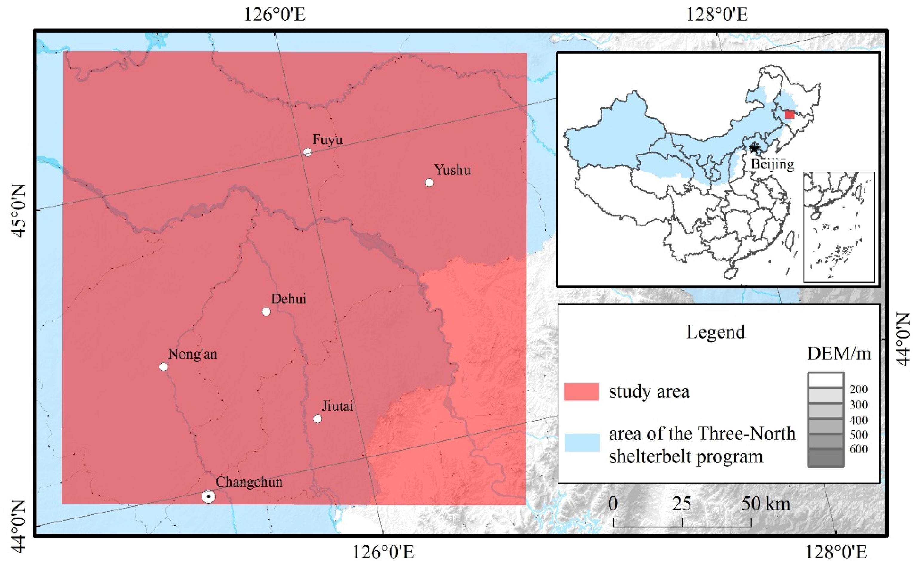
2.1. Study Area

The study area was located in Songnen Plain in the midwestern Jilin Province in north-eastern China (Figure 1). The climate in the area is a temperate, semi-humid, continental climate with annual precipitation of 660 mm and annual average temperature of 5 °C. The study area represents typical areas included in the Three-North Shelterbelt Program, a massive reforestation program with the objective to reduce the infestation of sandstorms in northern China. This area is also one of the main grain-producing regions in China and is known as one of the three most renowned corn belts in the world. Farmland shelterbelt construction started in the 1950s and was well established in the study area; the shelterbelt has been providing important protection against wind erosion to secure the stable production of grain crops [30]. However, the construction of the shelterbelt was undertaken by local people at different time periods, largely without consistent planning based on scientific data. As such, the early shelterbelt forests offered only limited protection against wind erosion. Following the implementation of the Three-North Shelterbelt Program in 1978, regional farmland shelterbelt construction underwent rapid development, and now networks of farmland shelterbelts have dramatically reduced sandstorm severity and frequency. Currently, the farmland shelterbelt established over the last 30 years is undergoing a stage of renewal and improvement.

2.2. Data Source

2.2.1. Selection of Remote Sensing Images

The canopy width of a typical farmland shelterbelt is approximately 20 m. Therefore, for the accurate extraction of shelterbelt information, the spatial resolution of remote sensing imagery should be ≤30 m. In addition, a continuous sequence of remote sensing images was needed for our analysis as the farmland shelterbelts were established as early as 1950. Images from the Landsat series (i.e., Landsat-5, Landsat-7, and Landsat-8) were considered suitable for this study.

In multispectral images, shelterbelts and crops have similar spectral characteristics during growing seasons with a closed crop canopy. However, between May and early to- mid June, when the tree leaves have fully emerged and the crops have not yet fully grown, the spectrum characteristics of shelterbelt trees can be differentiated from crop lands. This time window was optimal for extracting shelterbelt information with multispectral satellite images [20]. The Landsat images available between 1 May and 15 June each year since 1984 were acquired (

Table 1. The available data from Landsat image series in the study area.

Year	Data Source	Date (Month-Day)	Cloud Cover (%)
1984	No available
1985	Landsat-5	28 May	0
1986	Landsat-5	31 May	8
1987	Landsat-5	18 May	0
1988	Landsat-5	20 May	3
1989	No available
1990	No available
1991	Landsat-5	14 June	2
1992	No available
1993	No available
1994	Landsat-5	21 May	19
1995	Landsat-5	9 June	30
1996	Landsat-5	11 June	5
1997	Landsat-5	14 June	0
1998	Landsat-5	16 May	0
1999	Landsat-5	4 June	4
2000	No available
2001	Landsat-5	9 June	10
2002	No available
2003	Landsat-5	14 May	0
2004	Landsat-5	1 June	0
2005	Landsat-5	19 May	0
2006	Landsat-5	6 May	7
2007	Landsat-5	10 June	20
2008	Landsat-5	12 June	0
2009	Landsat-5	14 May	0
2010	Landsat-5	1 May	1
2011	Landsat-5	5 June	3
2012	No available
2013	Landsat-8	25 May	0
2014	Landsat-8	13 June	0
2015	Landsat-8	15 May	0
2016	Landsat-8	17 May	2
2017	Landsat-8	5 June	1
2018	Landsat-8	23 May	6
2019	No available
2020	Landsat-8	28 May	1
2021	No available

). The data were obtained from the Institute of Remote Sensing and Digital Earth, Chinese Academy of Sciences (Available online: http://eds.ceode.ac.cn (accessed on 13 July 2021)) and the United States Geological Survey (Available online: https://glovis.usgs.gov (accessed on 13 July 2021)). After reviewing the collection of remote sensing imagery for the study area, a two-year interval was determined as the monitoring period. Therefore, the following images in Table 1 were chosen to estimate the shelterbelt age based on the time series method: 28 May 1985, 18 May 1987, 14 June 1991, 9 June 1995, 14 June 1997, 4 June 1999, 14 May 2003, 19 May 2005, 10 June 2007, 14 May 2009, 5 June 2011, 25 May 2013, 15 May 2015, 5 June 2017 and 28 May 2020. The clouds in the images in 1995 and 2007 were heavy, so these images had to be interpolated. There were no suitable remote sensing images available in 1989 and 1993, so these had to be predicted. There were no suitable remote sensing images available in 2019 and 2021, so the image in 2019 was replaced by one from 2020.

Geometric corrections and radiometric calibration were accomplished using ENVI5.3 software. The topographic maps (scale 1:100,000) from the 1980s were used as reference data, and the ground control points were selected to register the Landsat-5 TM image acquired on 28 May 1985. Based on the corrected remote sensing image, the Landsat-5 image of the following year was corrected, and the process was repeated until the correction of all the images was completed. The positional deviation between the corrected image and the reference image was controlled to less than half a pixel.

Radiometric calibration was performed to convert the digital number values into top-of-atmosphere (TOA) reflectance using the corresponding radiometric calibration formula and radiometric rescaling coefficients provided in the metadata file that was delivered with the Level1 product [31].

2.2.2. Extraction of Vector Information in the Farmland Shelterbelt

Farmland shelterbelts were characterized as linear features with trees in regular network structures in areas with cultivated land. The reflective spectrum characteristics of shelterbelt features were sufficiently discernible in the Landsat images acquired on the optimal dates. Using the Landsat-8 standard pseudo-color image from 28 May 2020 as a base map, the features of the farmland shelterbelts were clearly identifiable as linear, red, and regular structures. Vector data of the farmland shelterbelt within the study area were obtained through manual interpretation via a computer interface using ArcMap software. The manual interpretation rules were defined as follows: (1) the shelterbelt was extracted as a linear vector; (2) it was interrupted at the intersection point of two or more shelterbelts; (3) it should keep the continuity of the gaps of the shelterbelt; and (4) the vector line should be drawn in the middle of the shelterbelt. Field validation was performed in early June 2020. A total of 243 shelterbelts were observed during the field validation, of which 233 shelterbelts were correctly interpreted. Field investigation revealed that the precision of the results was >95%. The shelterbelts failing to be accurately interpreted were those planted less than two years before the study.

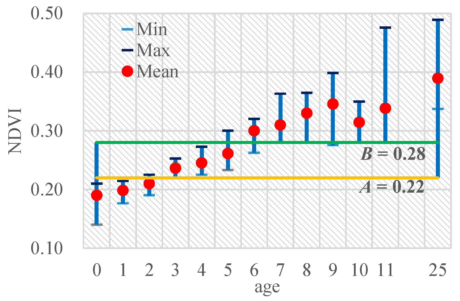
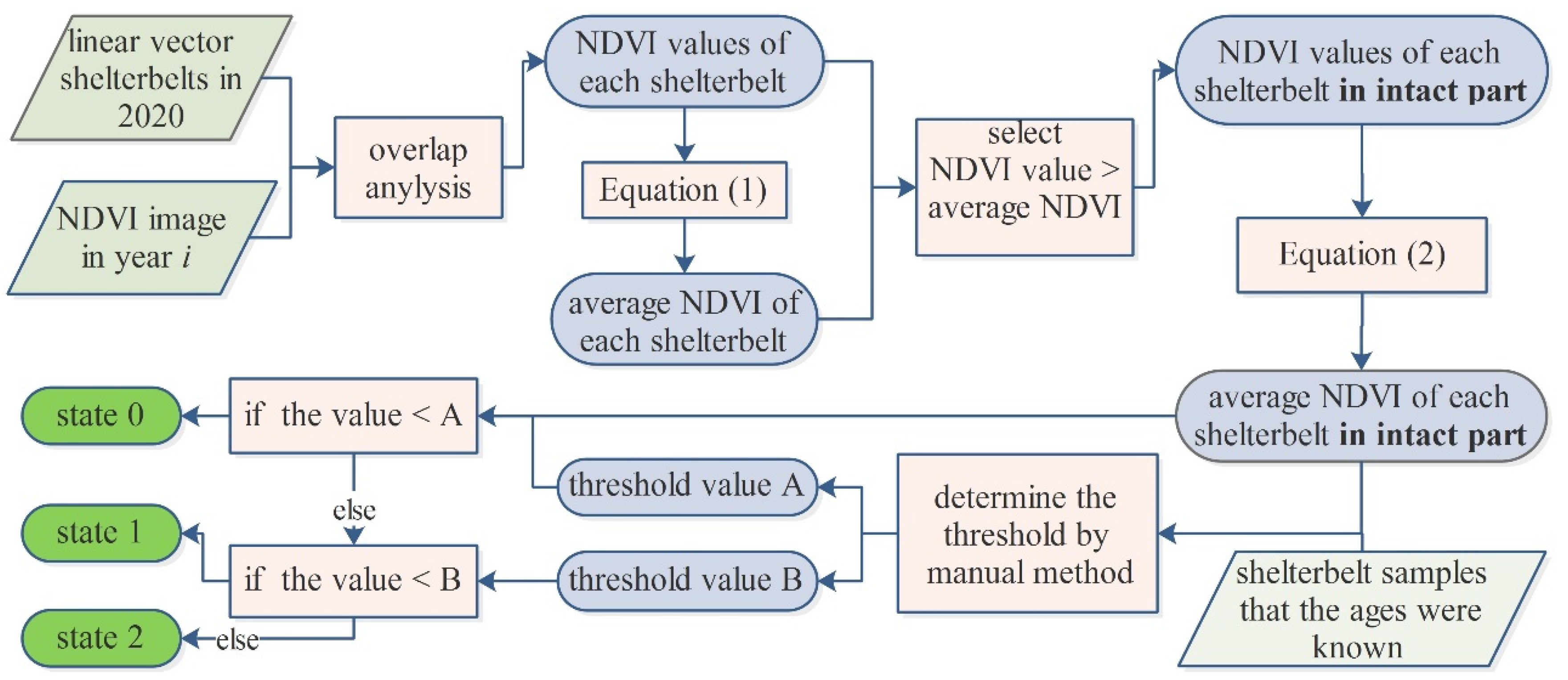
2.3. Dividing Shelterbelts into Three States Using a Single Remote Sensing Image

NDVI was used to divide the states of the shelterbelts in each single image. It was calculated by the TOA reflectance values of the red and near-infrared bands of each image. As shown in Figure 2, the dividing method consisted of three steps.

Firstly, the NDVI values that overlapped with the vector shelterbelts in each year were extracted with reference to Deng et al. (2013) [32]. The average NDVI value of each shelterbelt in each year ($\overline{NDV{I}_{ij}}$) was calculated by the following formula:

$$\overline{NDV{I}_{ij}}={\displaystyle \sum }_{k=1}^{M}NDV{I}_{ijk}/M$$

(1)

where i is the year of the image, j is the identification number of each shelterbelt, k is the serial number of the pixel in each shelterbelt, and M is the total number of NDVI values in each shelterbelt.

The NDVI values greater than $\overline{NDV{I}_{ij}}$ in each shelterbelt were selected as the intact parts of a shelterbelt. The average NDVI value of each intact part ($\overline{ANDV{I}_{ij}}$) was taken as the growth-state index, which was calculated by the following formula:

$$\overline{ANDV{I}_{ij}}={\displaystyle \sum }_{l=1}^{N}NDV{I}_{ijl}/N$$

(2)

where l is the serial number of pixels that are greater than $\overline{NDV{I}_{ij}}$ in each shelterbelt, $NDV{I}_{ijl}$ is the NDVI value that is greater than $\overline{NDV{I}_{ij}}$, and N is the total number of NDVI values greater than $\overline{NDV{I}_{ij}}$.

Finally, a threshold was used to divide the shelterbelts into three states: state 0 represented that the shelterbelt had no vegetation feature in the image and could not yet be monitored; state 1 represented that the shelterbelt had weak vegetation features and could be monitored with low accuracy; and state 2 represented that the shelterbelt had clear vegetation features and could accurately be monitored). The states of the shelterbelts in each image were divided using the following rules:

$$\begin{array}{l}\mathrm{If} (\overline{ANDV{I}_{ij}}\le A, {\mathrm{state}}_{ij}=0\\ \mathrm{Else} \mathrm{if} A<\overline{ANDV{I}_{ij}}\le B, {\mathrm{state}}_{ij}=1\\ \mathrm{Else} {\mathrm{state}}_{ij}=2\end{array}$$

where A is the threshold between state 0 and 1 in year i, and B is the threshold between state 1 and 2 in year i.

Thresholds A and B were manually determined by investigating the NDVI values of shelterbelts, for which the year of planting was known. Using the image from 28 May 2020, an example is as follows. The NDVI values (max, min, and mean) of the intact parts of the shelterbelts of different ages are shown in Figure 3. It showed that the spectral characteristics of the farmland shelterbelts were similar when the shelterbelt age was >6 years. The values for shelterbelts that were 1–2 years old were close to those of bare soil (age = 0), but the difference between 1–2 years old and >2 years old was evident. The NDVI of shelterbelts that were 3–4 years old and those that were >6 years old were even more evident. Therefore, 0.22 was selected as the threshold A in 2020, and 0.28 was selected as the threshold B.

2.4. Establishing a Three-Stage Growth Process Using Time Series Remote Sensing Image

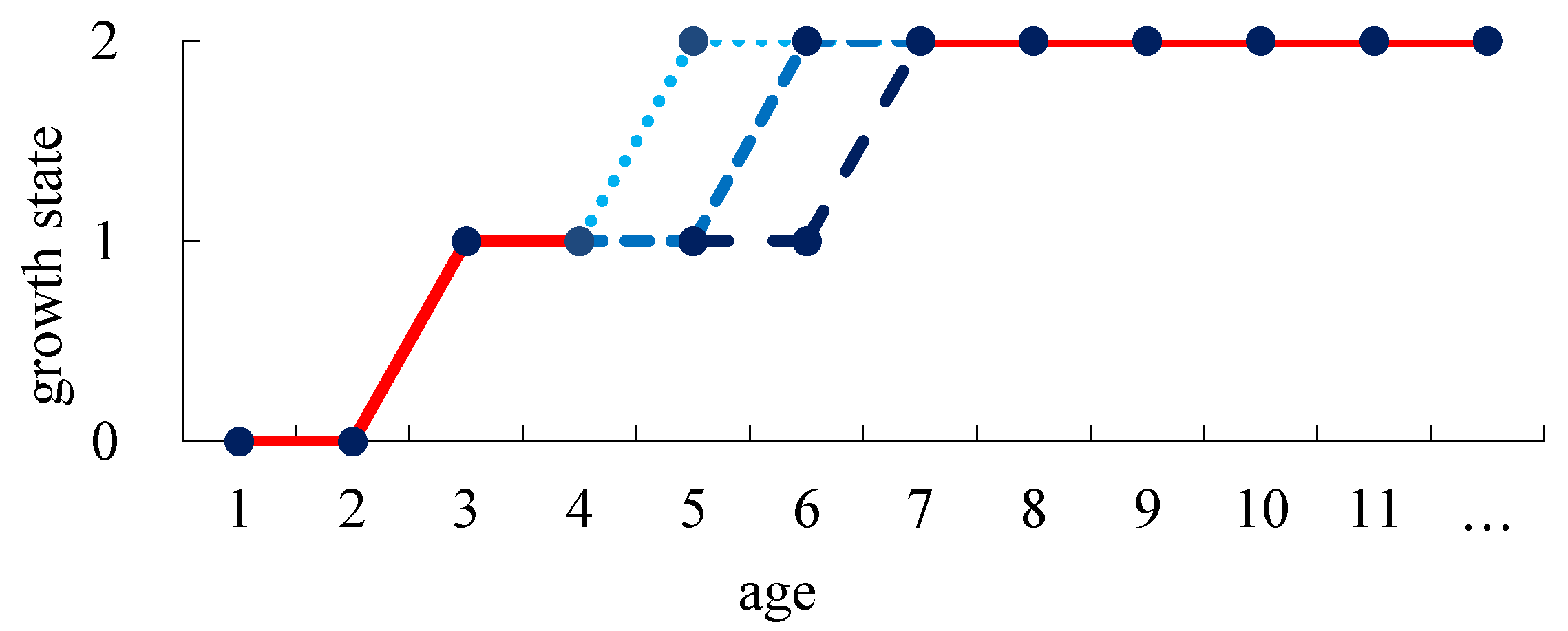
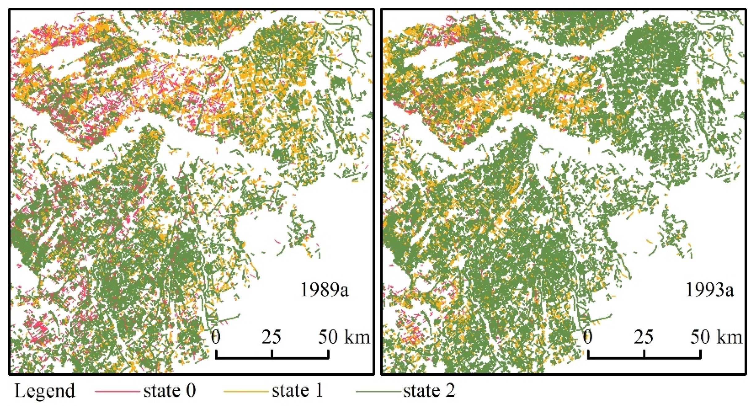
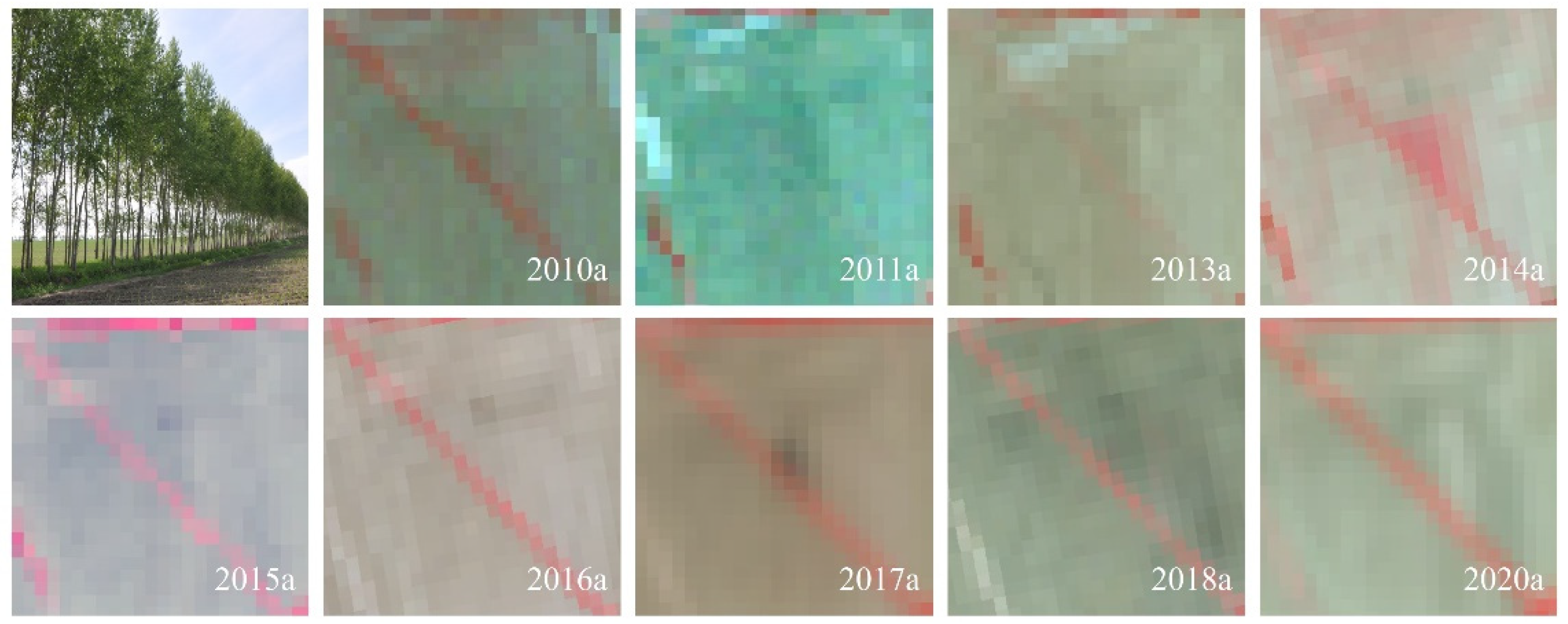
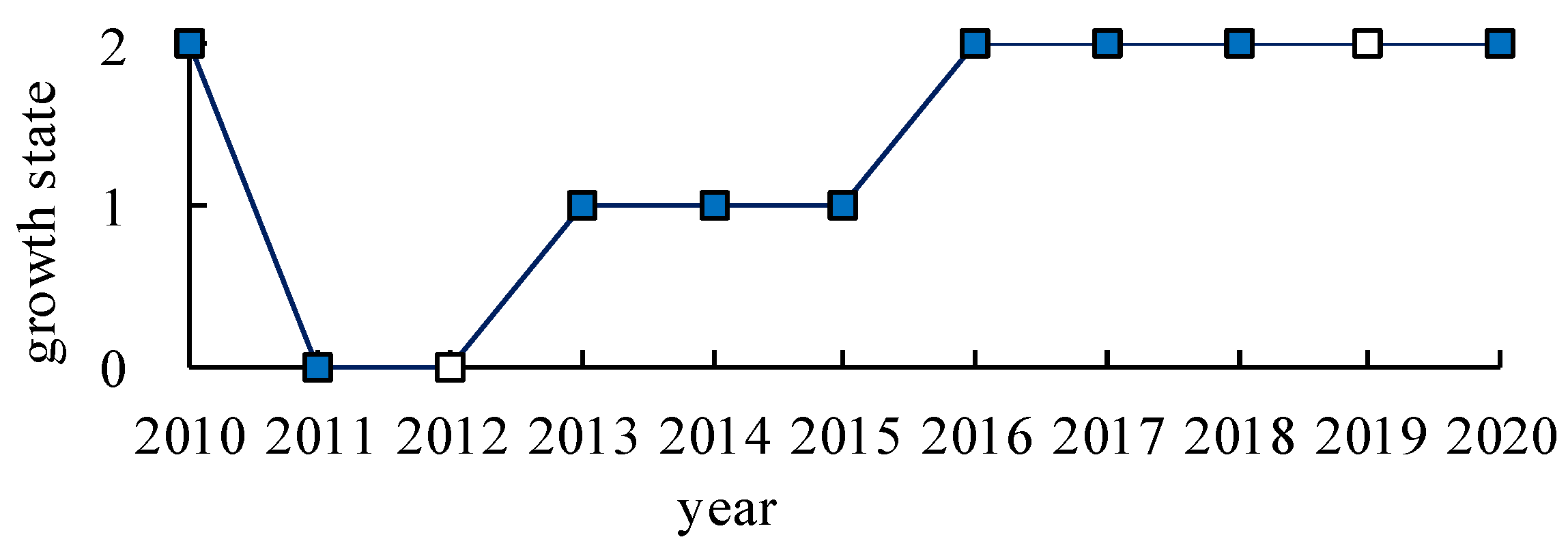
2.4.1. Shelterbelt Growth Process from Time Series Images

A shelterbelt age could only be divided into two states using a single multispectral image. To overcome this limitation, multitemporal remote sensing images were considered. A shelterbelt planted in 2011 was used to illustrate the changes in spectral characteristics with increasing age (Figure 4; there were no suitable images in 2012 and 2019). The shelterbelt (the red linear object in Figure 4) was evident in 2010 and disappeared in the image from 2011. A weak feature was apparent in 2013 and then became increasingly identifiable from 2014 to 2020.

Based on the three states of farmland shelterbelts that were determined from a single remote sensing image, the growth process of the shelterbelt shown in Figure 4 are expressed in Figure 5. According to remote sensing monitoring, shelterbelt growth attains each state (i.e., states 0, 1, and 2) successively. The duration of a shelterbelt in state 0 and state 1 was 2 and 3 years, respectively. A shelterbelt in state 2 was considered to commence from the sixth year after planting.

2.4.2. Three-Stage Growth of Farmland Shelterbelt Derived from Time Series Remote Sensing Images

In order to describe the shelterbelt growth process in a more general way, more than 100 shelterbelts were randomly selected to analyze their growth processes. We found that there could be three separate cases in the process of farmland shelterbelt construction: (1) the shelterbelt was constructed for the first time; that is, it was initially 0 and then gradually changed from 0 to 2 after planting; (2) the shelterbelt was renewed soon after the old shelterbelt was cut down; that is, it was initially 2 and then gradually changed from 0 to 2 following renewal; and (3) the shelterbelt was not renewed soon after the old shelterbelt was cut down; that is, it was initially 2 and then changed to 0 (it would gradually change from 0 to 2 if renewed later).

In the above three cases, as long as the farmland shelterbelt was planted, the growth process of the most shelterbelts followed the following three stages (Figure 6). Stage A: In the early period (generally 2 years after planting), the shelterbelt was difficult to observe in remote sensing imagery (state was 0). Stage B: After growing to a certain state (generally 2–4 years after planting), the shelterbelt was monitored in remote sensing images but not always clearly (state was (1). Stage C: Following continued growth (generally 5–7 years after planting), the shelterbelt was identified easily in remote sensing imagery (state was (2). The above represents a general description of the growth process of farmland shelterbelts, which we refer to as the three-stage growth process of farmland shelterbelts.

The three-stage growth process of farmland shelterbelts determined from time series remote sensing images represented an ideal status. In practical application, it may be affected by other factors, especially cloud cover, which may cause deviations in the simulation of the shelterbelt growth process. If clouds were present, shelterbelts in state 1 could be misclassified as 0, or shelterbelts in state 2 could be misclassified as 0 or 1. According to the three-stage growth process in Figure 6, the following rules were developed to improve prediction accuracy:

If the growth state in the year (i) is 2, then the state in the previous period (i − 2) could not be 0. Farmland shelterbelts could not change directly from 0 to 2 in two years. In such a situation, which could be the result of interference by clouds, the 0 in the previous period (i − 2) would be revised to either 1 or 2.

If the growth state in the year (i) is 2, then the state in the subsequent period (i + 2) could not be 1. Farmland shelterbelts could not change directly from 2 to 1 in two years. In such a situation, which could be attributed to the presence of thin cloud cover or the decline in a mature shelterbelt, the 1 in the subsequent period (i + 2) would be revised to 2.

The prediction of shelterbelt states in years with missing imagery could also be made according to the three-stage growth process, as shown in

Table 2. Growth-state prediction for missing years based on the three-stage growth process over a two-year period.

	i − 2	Missing Year (i)	i + 2
Growth state	0	0	0
	0	if I − 4 = 2, statei = 1; if I + 4 = 1, statei = 0	1
	0	1	2
	1	×	0
	1	×	1
	1	1 or 2	2
	2	0 or 2	0
	2	0	1
	2	2	2

.

2.5. Algorithm for the Identification of Shelterbelt Ages Based on Time Series Remote Sensing Images

If the two-year interval was determined as the monitoring period, the age of the shelterbelt j (AGE_j) in monitoring year X could be determined by the following algorithm:

$$AG{E}_j=\left(1 or 2\right)+\left(X-Y_i\right)$$

(3)

where X is the year being monitored and Y_i is the nearest year when the jth shelterbelt had been classified as state 0. For example, in the monitoring year 2010 (X = 2010), one shelterbelt had been classified as state 0 in year 1998 (Y_i = 1998). The age of this shelterbelt should have been 13 or 14. As there was no suitable image available in 2019, the image from 2020 was substituted. Therefore, the following special condition existed: if state₂₀₁₇ = 2 and state₂₀₂₀ = 1, the shelterbelt age was 2–3.

3. Results

3.1. Modification and Predication of the Shelterbelt States

Following the steps in Figure 2, $\overline{ANDVI}$ of the shelterbelts in each image were calculated by Formulas (1) and (2). The threshold values were determined by analyzing the shelterbelts for which the years of planting were known. The states of the shelterbelts were divided using threshold values A and B. The growth states of the shelterbelts in all monitored years were divided successively.

In the results, large areas of shelterbelts in state 0 were distributed in 1995, and the large area of shelterbelts in state 1 were distributed in 2007. This was due to the cloud cover in these two years. Especially in 1995, the cloud cover area reached up to 30%. In order to reduce the impact of the cloud cover, the shelterbelt states in each period, especially in 1995 and 2007, were modified using the rules established by the three-stage growth process. According to rule 1), the shelterbelts in states 0 in 1995 were revised to either 1 or 2 based on their states in 1997 and 1999, and the shelterbelts in state 0 in 2007 were revised to either 1 or 2 based on their states in 2009 and 2011. According to rule 2), the shelterbelts in state 1 in 1995 were revised to 2 based on their states in 1991 and 1994 (the states in 1994 replaced 1993 due to there being no suitable image available in 1993), and the shelterbelts in state 1 in 2007 were revised to 2 based on their states in 2003 and 2005. The modification results in the areas with cloud cover are shown in Figure 7. It indicated that some shelterbelts, which were divided into state 0 or 1 in the cloud cover areas, were adjusted into state 2 after modification.

In addition, the shelterbelt states in 1989 and 1993 were not determined as there were no suitable remote sensing images available. The states of some shelterbelts in 1989 and 1993 were predicted using the rule in Table 2. The shelterbelt states in 1989 were predicted from their states in 1987 and 1991, and the shelterbelt states in 1993 were predicted from their states in 1991 and 1995. The predicted results are shown in Figure 8.

3.2. Identification Result and Validation

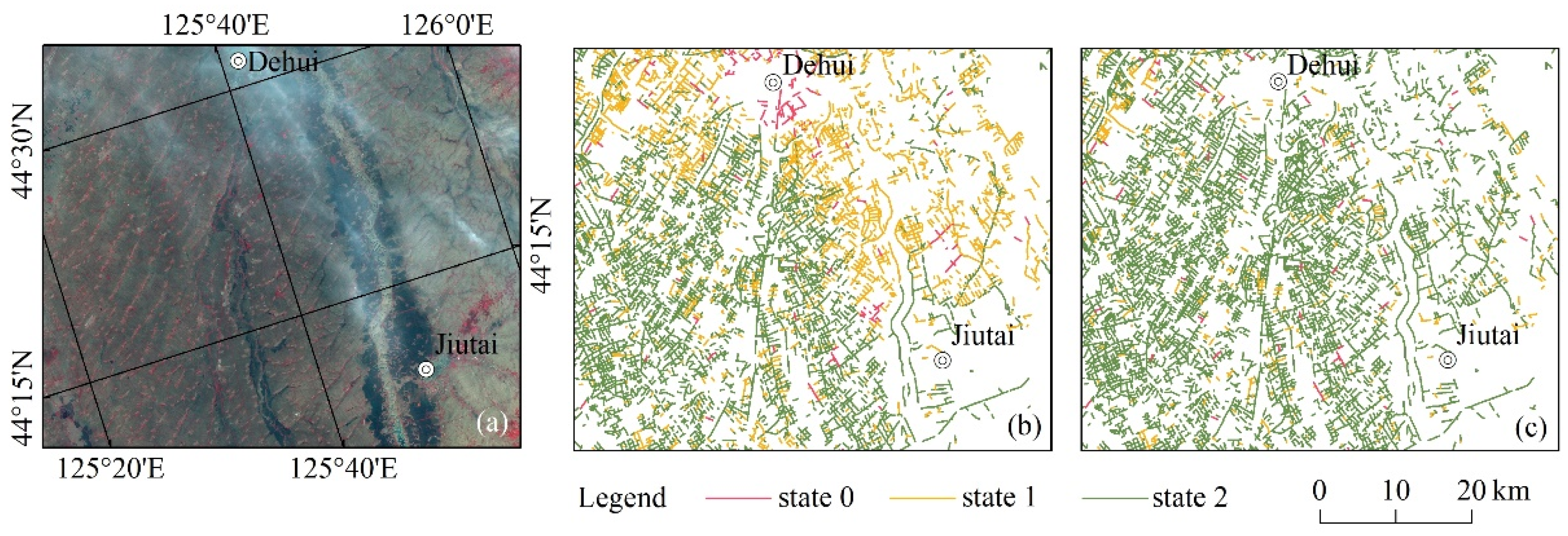
3.2.1. Identification Result

Based on the modification and prediction results of the shelterbelt states in each monitoring year, the shelterbelt ages in 2020 were identified using the algorithm. The result is presented in Figure 9. Given the two-year monitoring period, the monitoring error was 1 year. The minimum age that could be monitored was 2–3 years, and the maximum age was 36–37 years; ages that exceeded 37 could not be identified as no suitable images were available.

3.2.2. Validation

The following formula was used to analyze the accuracy of the shelterbelt ages derived from the remote sensing images:

$$RE=n/N$$

(4)

where RE is the accuracy rate, n is the number of correct identifications, and N is the total number of samples.

The shelterbelt heights in the samples were measured using a portable laser range finder in the field. A regression model between tree height and age in the study area, established by [33], was used to calculate the actual age of a shelterbelt based on the field measurements. To ensure the accuracy of the reference data, the age of each shelterbelt was validated through visual interpretation from the time series remote sensing images to determine the year of planting or updating. Of the total number of samples (N = 243), within the error range of 1 year, the ages of 167 shelterbelts were identified correctly. The identification accuracy of their ages based on the two-year monitoring periods was 68.7%.

According to phase-directional management [34], the shelterbelt ages in the study area were classified, as follows, to be further validated: generated phase (1–3 years after planting), pre-maturity phase (4–15 years after planting), protective maturity phase (16–33 years after planting), and regenerated phase (>33 years after planting). The accuracy was evaluated using a confusion matrix. The results are presented in

Table 3. Confusion matrix between estimated data and ground/truth data.

	Ground Truth Data
	Class	1–3a	4–15a	16–33a	>33a	Total	Commission
Estimated data	1–3a	23	10	0	0	33	30.3%
	4–15a	5	103	5	2	115	10.4%
	16–33a	0	15	33	3	51	35.3%
	>33a	3	13	4	24	44	45.5%
	Total	31	141	42	29	243
	Omission	25.8%	27.0%	21.4%	17.2%

.

As shown in Table 3, the misclassified shelterbelts were concentrated around adjacent classes. The column data in Table 3, reflecting the omission error of each class, showed that the average omission error was 22.9%. The reason was due to the year of shelterbelt planting (state 0) having not been identified. This may have been due to the NDVI values of these shelterbelts being influenced by neighboring vegetation pixels, or because the threshold between the state 0 and 1 was slightly lower than in reality. The row data in Table 3 shows the commission errors, which reflect those shelterbelts that had been assigned incorrectly to certain planting years. The smallest commission error among the various classes was for a shelterbelt with an age of 4–15 years. The commission error was larger in the other age classes and was >45% for a shelterbelt with an age of >33 years. The reason for this was that the ages had been calculated from the latest year forward; thus, the error would be cumulative. Most shelterbelts for which the planting year was not correctly identified were, therefore, incorrectly assigned to this class, especially those influenced by cloud cover.

4. Discussion

4.1. Uncertainty Analysis

Some factors affected the identification accuracy: (1) The impact of missing images and cloud cover. Although efforts had been made to overcome these problems by modification and prediction using the three-stage growth process, some shelterbelts were still misclassified, especially in the early monitoring years with more frequently missing data. (2) The three-stage growth process was suitable for most shelterbelts, but special shelterbelts such as those with larger widths could have exhibited spectral characteristics of vegetation in the second year following planting, which could have caused omission errors. Moreover, mature shelterbelts with short lengths or poor growing conditions could have been identified as state 0 or 1, which could have caused commission errors. (3) The threshold segmentation method also caused a certain degree of confusion, as there was no absolute boundary between state 0 and 1.

To reduce the uncertainties and improve overall accuracy, remote sensing images obtained from multiple sources and an annual monitoring period should be considered in future work. In particular, the Ice, Cloud, and Land Elevation Satellite-2 (ICESat-2; [35]) and the Global Ecosystem Dynamics Investigation (GEDI; [36]) could provide useful data, as they offer unprecedented opportunities to establish geodetic elevation distributions of global topographic surfaces and canopy heights [37]. Data fusion from active and multispectral sensors (e.g., Landsat, Sentinel-2) could improve the characterization of shelterbelt ages. To improve the classification accuracy of shelterbelt growth states, a more scientific approach that requires less human interpretation should be considered in the future to determine appropriate thresholds. We also found that the planting structure of farmland shelterbelts (e.g., the width and spacing of the trees) affected the growth state estimation, and these factors should also be considered in future research regarding the identification process. The proposed method will be optimized in future work, and thus the accuracy will be further improved.

4.2. Method Comparison

Remote sensing methods have significant potential and a wide range of applications in forest age mapping [38]. Optical remote sensing, as one of the most commonly used data types, has been an important resource for regional forest age mapping through its use of forest spectral characteristics and multi-temporal observation data [39]. However, remote sensing signals, such as from Landsat TM signal, have not been significantly sensitive enough to determine forest ages [13,40], so it has been difficult to infer forest age directly from optical remote sensing data. Active sensors such as LiDAR have shown great potential for the monitoring of structural attributes in forests [41]. However, they have not been able to directly retrieve tree age.

Monitoring via time series remote sensing images could address the aforementioned problems. In this research, a method for monitoring shelterbelt age was developed based on time series Landsat remote sensing images. Most studies concerning forest age using time series monitoring have used pixel-based image analysis [42]. For monitoring objects in stands of similar age, Fujiki et al. (2016) extracted stand ages from a change-detection analysis using Landsat time series images superimposed with the derived stand ages on the segments that had been classified by object-based image analysis, using WorldView-2 [43]. Farmland shelterbelts have relatively uniform planting structures, so an object-based image analysis may be a better choice. In this paper, each shelterbelt was digitized into linear vector objects, which were taken as a unit to identify the shelterbelt state. Furthermore, the method involved the establishment of a general monitoring model of the shelterbelt growth process, which may be feasible for large-scale identification of shelterbelt ages in other regions. Therefore, this method demonstrated considerable potential, as compared to other methods used in shelterbelt age identification by remote sensing.

It should be noted that the shelterbelt age identified by this method represented the number of years after planting; generally, a tree is approximately 2–3 years old before it is planted in these shelterbelts. The proposed was applicable to similarly aged, single-species shelterbelts with relatively uniform planting structures. To determine the accuracy of this method for shelterbelts of mixed ages, mixed species shelterbelts should be evaluated.

4.3. Implications of the Result

The division of the shelterbelt management phase is crucial for the appropriate management of a shelterbelt. Jiang and Zhu (2002) proposed the concept of phase-directional management for protective plantations [34]. Shelterbelt age is an important parameter to determine the management phases. Therefore, the management phases of shelterbelts can be classified on a regional scale based on the shelterbelt age extracted using this method.

The shelterbelt age can also be used to estimate aboveground biomass (AGB) based on its relationship with the stand age. Since AGB have been shown to be strongly related to successional age [44], it may be possible to use this information to estimate the spatial distribution of AGB. Some researchers have estimated the AGB based on forest biomass–age relationships [45,46]. The AGB of the shelterbelts can also be mapped based on the relationship using the shelterbelt age data.

5. Conclusions

In conclusion, this research established a generalized shelterbelt growth process and developed a method for the accurate estimation of shelterbelt ages based on multitemporal Landsat remote sensing images. The method was successfully used to determine shelterbelt ages in the midwestern Jilin Province in China. The proposed method provides a cognitive mechanism and application model for the identification of shelterbelt age using remote sensing imagery. The data could be used to support more precise management of shelterbelts and the estimation of carbon flux in shelterbelt ecosystems.

References

1. Brandle, J.; Hodges, L.; Zhou, X. Windbreaks in North American agricultural systems. Agrofor. Syst. 2004, 61–62, 65–78. [Google Scholar] [CrossRef]
2. Stange, C. Windbreak Management; Papers in Natural Resources; University of Nebraska-Lincoln: Lincoln, NE, USA, 1996; p. 124. [Google Scholar]
3. Helama, S. Expressing Tree-Ring Chronology as Age-Standardized Growth Measurements. For. Sci. 2015, 61, 817–828. [Google Scholar] [CrossRef]
4. Sun, J.; Hamel, J.-F.; Gianasi, B.L.; Mercier, A. Age determination in echinoderms: First evidence of annual growth rings in holothuroids. Proc. R. Soc. B Boil. Sci. 2019, 286, 20190858. [Google Scholar] [CrossRef] [PubMed] [Green Version]
5. Nascimbene, J.; Marini, L.; Motta, R.; Nimis, P.L. Influence of tree age, tree size and crown structure on lichen communities in mature Alpine spruce forests. Biodivers. Conserv. 2009, 18, 1509–1522. [Google Scholar] [CrossRef]
6. Trotsiuk, V.; Hobi, M.; Commarmot, B. Age structure and disturbance dynamics of the relic virgin beech forest Uholka (Ukrainian Carpathians). For. Ecol. Manag. 2012, 265, 181–190. [Google Scholar] [CrossRef]
7. Dey, D.C.; Dwyer, J.; Wiedenbeck, J. Relationship between Tree Value, Diameter, and Age in High-Quality Sugar Maple (Acer saccharum) on the Menominee Reservation, Wisconsin. J. For. 2017, 115, 397–405. [Google Scholar] [CrossRef]
8. Briseño-Reyes, J.; Corral-Rivas, J.J.; Solis-Moreno, R.; Padilla-Martínez, J.R.; Vega-Nieva, D.J.; López-Serrano, P.M.; Vargas-Larreta, B.; Diéguez-Aranda, U.; Quiñonez-Barraza, G.; López-Sánchez, C.A. Individual Tree Diameter and Height Growth Models for 30 Tree Species in Mixed-Species and Uneven-Aged Forests of Mexico. Forests 2020, 11, 429. [Google Scholar] [CrossRef] [Green Version]
9. Ojoatre, S.; Zhang, C.; Hussin, Y.A.; Kloosterman, H.E.; Ismail, M.H. Assessing the Uncertainty of Tree Height and Aboveground Biomass from Terrestrial Laser Scanner and Hypsometer Using Airborne LiDAR Data in Tropical Rainforests. IEEE J. Sel. Top. Appl. Earth Obs. Remote Sens. 2019, 12, 4149–4159. [Google Scholar] [CrossRef] [Green Version]
10. Yang, Z.; Liu, Q.; Luo, P.; Ye, Q.; Duan, G.; Sharma, R.; Zhang, H.; Wang, G.; Fu, L. Prediction of Individual Tree Diameter and Height to Crown Base Using Nonlinear Simultaneous Regression and Airborne LiDAR Data. Remote Sens. 2020, 12, 2238. [Google Scholar] [CrossRef]
11. Zhou, X.; Wang, W.; Di, L.; Lu, L.; Guo, L. Estimation of Tree Height by Combining Low Density Airborne LiDAR Data and Images Using the 3D Tree Model: A Case Study in a Subtropical Forest in China. Forests 2020, 11, 1252. [Google Scholar] [CrossRef]
12. Kobal, M.; Hladnik, D. Tree Height Growth Modelling Using LiDAR-Derived Topography Information. ISPRS Int. J. Geo-Inf. 2021, 10, 419. [Google Scholar] [CrossRef]
13. Yang, X.; Liu, Y.; Wu, Z.; Yu, Y.; Li, F.; Fan, W. Forest age mapping based on multiple-resource remote sensing data. Environ. Monit. Assess. 2020, 192, 734. [Google Scholar] [CrossRef] [PubMed]
14. Dye, M.; Mutanga, O.; Ismail, R. Combining Spectral and Textural Remote Sensing Variables Using Random Forests: Predicting the Age of Pinus Patula Forests in KwaZulu-Natal, South Africa. J. Spat. Sci. 2012, 57, 193–211. [Google Scholar] [CrossRef]
15. Chemura, A.; van Duren, I.; van Leeuwen, L.M. Determination of the Age of Oil Palm from Crown Projection Area Detected from WorldView-2 Multispectral Remote Sensing Data: The Case of Ejisu-Juaben District, Ghana. ISPRS-J. Photogramm. Remote Sens. 2015, 100, 118–127. [Google Scholar] [CrossRef]
16. Cao, X.; Liu, Y.; Liu, Q.; Cui, X.; Chen, X.; Chen, J. Estimating the age and population structure of encroaching shrubs in arid/semiarid grasslands using high spatial resolution remote sensing imagery. Remote Sens. Environ. 2018, 216, 572–585. [Google Scholar] [CrossRef]
17. Qiao, C.; Sun, R.; Xu, Z.; Zhang, L.; Liu, L.; Hao, L.; Jiang, G. A Study of Shelterbelt Transpiration and Cropland Evapotranspiration in an Irrigated Area in the Middle Reaches of the Heihe River in Northwestern China. IEEE Geosci. Remote Sens. Lett. 2015, 12, 369–373. [Google Scholar] [CrossRef]
18. Xing, Z.F.; Li, Y.; Deng, R.X.; Zhu, H.L.; Fu, B.L. Extracting Farmland Shelterbelt Automatically Based on ZY-3 Remote Sensing Images. Sci. Silv. Sin. 2016, 52, 11–20. [Google Scholar]
19. Zheng, X.; Zhu, J.; Xing, Z. Assessment of the effects of shelterbelts on crop yields at the regional scale in Northeast China. Agric. Syst. 2016, 143, 49–60. [Google Scholar] [CrossRef]
20. Deng, R.X.; Li, Y.; Xu, X.L.; Wang, W.J.; Wei., Y.C. Remote estimation of shelterbelt width from SPOT5 imagery. Agrofor. Syst. 2017, 91, 161–172. [Google Scholar] [CrossRef]
21. Yu, T.; Liu, P.; Zhang, Q.; Ren, Y.; Yao, J. Detecting Forest Degradation in the Three-North Forest Shelterbelt in China from Multi-Scale Satellite Images. Remote Sens. 2021, 13, 1131. [Google Scholar] [CrossRef]
22. De Fries, R.S.; Townshend, J.R.G. NDVI-Derived Land Cover Classifications at Global Scale. Int. J. Remote Sens. 1994, 15, 3567–3586. [Google Scholar] [CrossRef]
23. Loveland, T.R.; Reed, B.C.; Brown, J.F.; Ohlen, D.O.; Zhu, Z.; Yang, L.; Merchant, J.W. Development of a global land cover characteristics database and IGBP DISCover from 1 km AVHRR data. Int. J. Remote Sens. 2000, 21, 1303–1330. [Google Scholar] [CrossRef]
24. Pan, Z.; Huang, J.; Zhou, Q.; Wang, L.; Cheng, Y.; Zhang, H.; Blackburn, G.A.; Yan, J.; Liu, J. Mapping crop phenology using NDVI time-series derived from HJ-1 A/B data. Int. J. Appl. Earth Obs. Geoinf. 2015, 34, 188–197. [Google Scholar] [CrossRef] [Green Version]
25. Guan, X.; Huang, C.; Liu, G.; Meng, X.; Liu, Q. Mapping Rice Cropping Systems in Vietnam Using an NDVI-Based Time-Series Similarity Measurement Based on DTW Distance. Remote Sens. 2016, 8, 19. [Google Scholar] [CrossRef] [Green Version]
26. Antonucci, S.; Rossi, S.; Deslauriers, A.; Morin, H.; Lombardi, F.; Marchetti, M.; Tognetti, R. Large-scale estimation of xylem phenology in black spruce through remote sensing. Agric. For. Meteorol. 2017, 233, 92–100. [Google Scholar] [CrossRef]
27. Khare, S.; Drolet, G.; Sylvain, J.-D.; Paré, M.C.; Rossi, S. Assessment of Spatio-Temporal Patterns of Black Spruce Bud Phenology across Quebec Based on MODIS-NDVI Time Series and Field Observations. Remote Sens. 2019, 11, 2745. [Google Scholar] [CrossRef] [Green Version]
28. Li, X.F.; Tian, Y.C.; Zheng, X.; Cong, J.X.; Song, L.N. Characterizing 40 Years of Natural Pinus Sylvestris Var. Mongolica Carbon Stocks in Northeast China Using Stand Age from Remote Sensing Time Series. Int. J. Remote Sens. 2020, 41, 2391–2409. [Google Scholar] [CrossRef]
29. Ji, Z.; Pan, Y.; Zhu, X.; Wang, J.; Li, Q. Prediction of Crop Yield Using Phenological Information Extracted from Remote Sensing Vegetation Index. Sensors 2021, 21, 1406. [Google Scholar] [CrossRef]
30. Shi, X.; Li, Y.; Deng, R. A method for spatial heterogeneity evaluation on landscape pattern of farmland shelterbelt networks: A case study in midwest of Jilin Province, China. Chin. Geogr. Sci. 2011, 21, 48–56. [Google Scholar] [CrossRef]
31. USGS. Available online: https://www.usgs.gov/landsat-missions/using-usgs-landsat-level-1-data-product (accessed on 13 March 2022).
32. Deng, R.; Li, Y.; Wang, W.; Zhang, S. Recognition of shelterbelt continuity using remote sensing and waveform recognition. Agrofor. Syst. 2013, 87, 827–834. [Google Scholar] [CrossRef]
33. Jiang, F.; Zhu, J.; Zeng, D.; Fan, Z.; Du, X.; Cao, Y. Management for Protective Plantations; China Forestry Publisher: Beijing, China, 2003; pp. 75–86. [Google Scholar]
34. Jiang, F.Q.; Zhu, J.J. Phase-Directional Management of Protective Plantations. I. Fundamentals. Chin. J. Appl. Ecol. 2002, 13, 1352–1355. [Google Scholar]
35. Markus, T.; Neumann, T.; Martino, A.; Abdalati, W.; Brunt, K.; Csatho, B.; Farrell, S.; Fricker, H.; Gardner, A.; Harding, D.; et al. The ice, cloud, and land elevation Satellite-2 (ICESat-2): Science requirements, concept, and implementation. Remote Sens. Environ. 2017, 190, 260–273. [Google Scholar] [CrossRef]
36. Dubayah, R.; Blair, J.B.; Goetz, S.; Fatoyinbo, L.; Hansen, M.; Healey, S.; Hofton, M.; Hurtt, G.; Kellner, J.; Luthcke, S.; et al. The global ecosystem dynamics investigation: High-resolution laser ranging of the Earth’s forests and topography. Sci. Remote Sens. 2020, 1, 100002. [Google Scholar] [CrossRef]
37. Liu, A.B.; Cheng, X.; Chen, Z.Q. Performance evaluation of GEDI and ICESat-2 laser altimeter data for terrain and canopy height retrievals. Remote Sens. Environ. 2021, 264, 112571. [Google Scholar] [CrossRef]
38. Xu, C.; Manley, B.; Morgenroth, J. Evaluation of modelling approaches in predicting forest volume and stand age for small-scale plantation forests in New Zealand with RapidEye and LiDAR. Int. J. Appl. Earth Obs. Geoinf. 2018, 73, 386–396. [Google Scholar] [CrossRef]
39. Lucas, R.M.; Xiao, X.; Hagen, S.; Frolking, S. Evaluating TERRA-1 MODIS data for discrimination of tropical secondary forest regeneration stages in the Brazilian Legal Amazon. Geophys. Res. Lett. 2002, 29, 42-1–42-4. [Google Scholar] [CrossRef] [Green Version]
40. Sader, S.A.; Waide, R.B.; Lawrence, W.T.; Joyce, A.T. Tropical forest biomass and successional age class relationships to a vegetation index derived from landsat TM data. Remote Sens. Environ. 1989, 28, 143–198. [Google Scholar] [CrossRef]
41. Hernández-Stefanoni, J.L.; Castillo-Santiago, M.Á; Mas, J.F.; Wheeler, C.E.; Andres-Mauricio, J.; Tun-Dzul, F.; George-Chacón, S.P.; Reyes-Palomeque, G.; Castellanos-Basto, B.; Vaca, R.; et al. Improving aboveground biomass maps of tropical dry forests by integrating LiDAR, ALOS PALSAR, climate and field data. Carbon Balance Manag. 2020, 15, 15. [Google Scholar] [CrossRef]
42. Ma, S.B.; Zhou, Z.F.; Zhang, Y.R.; An, Y.L.; Yang, G.B. Identification of Forest Disturbance and Estimation of Forest Age in Subtropical Mountainous Areas Based on Landsat Time Series Data. Earth Sci. Inform. 2022, 15, 321–334. [Google Scholar] [CrossRef]
43. Fujiki, S.; Okada, K.-I.; Nishio, S.; Kitayama, K. Estimation of the stand ages of tropical secondary forests after shifting cultivation based on the combination of WorldView-2 and time-series Landsat images. ISPRS J. Photogramm. Remote Sens. 2016, 119, 280–293. [Google Scholar] [CrossRef]
44. Read, L.; Lawrence, D. Recovery of Biomass Following Shifting Cultivation in Dry Tropical Forests of The Yucatan. Ecol. Appl. 2003, 13, 85–97. [Google Scholar] [CrossRef] [Green Version]
45. Liu, L.; Peng, D.; Wang, Z.; Hu, Y. Improving artificial forest biomass estimates using afforestation age information from time series Landsat stacks. Environ. Monit. Assess. 2014, 186, 7293–7306. [Google Scholar] [CrossRef] [PubMed]
46. Xu, B.; Guo, Z.; Piao, S.; Fang, J. Biomass carbon stocks in China’s forests between 2000 and 2050: A prediction based on forest biomass-age relationships. Sci. China Life Sci. 2010, 53, 776–783. [Google Scholar] [CrossRef] [PubMed]
Figure 1. Location of the study area.
Remotesensing 14 01457 g001
Figure 2. Flowchart of data processing in determining shelterbelt states.
Remotesensing 14 01457 g002
Figure 3. NDVI values of farmland shelterbelts with differing ages in 2020.
Remotesensing 14 01457 g003
Figure 4. Changes in spectral characteristics in different Landsat images of one farmland shelterbelt planted in 2011. (The images are composited by the standard pseudo color). For Landsat-5 images: red = 0.76–0.90 µm (near-infrared band); green = 0.63–0.69 µm (red band); blue = 0.52–0.60 µm (green band); For Landsat-8 images: red = 0.85–0.88 µm (near-infrared band); green = 0.64–0.67 µm (red band); blue = 0.53–0.59 µm (green band)).
Remotesensing 14 01457 g004
Figure 5. Growth process of the farmland shelterbelts shown in Figure 4.
Remotesensing 14 01457 g005
Figure 6. Generalized three-stage growth process of farmland shelterbelts (red line shows the stable growth process for farmland shelterbelts in 1–4 years and ≥7 years, and blue lines show the possible growth process for farmland shelterbelts in 5–6 years).
Remotesensing 14 01457 g006
Figure 7. The comparison of the farmland shelterbelt states before and after modification (a). the Landsat image with cloud cover; (b). the shelterbelt states without modification; (c). the shelterbelt states modified by the rules of three-stage growth process and shelterbelt states in the previous and subsequent years).
Remotesensing 14 01457 g007
Figure 8. The predicted farmland shelterbelt states in 1989 and 1993.
Remotesensing 14 01457 g008
Figure 9. Identification result of farmland shelterbelt ages in 2020 in the study area.
Remotesensing 14 01457 g009