Abstract
Natural rock slopes require accurate engineering–geological characterization to determine their stability conditions. Given that a natural rock mass is often characterized by a non-uniform fracture distribution, the correct, detailed, and accurate characterization of the discontinuity pattern of the rock mass is essential. This is crucial, for example, for identifying the possibility and the probability of kinematic releases. In addition, complete stability analyses of possible rockfall events should be performed and used to create hazard maps capable of identifying the most dangerous parts of a rock mass. This paper shows a working approach that combines traditional geological surveys and remote sensing techniques for engineering–geological investigations in a natural rock slope in Northern Italy. Discontinuities were identified and mapped in a deterministic way by using semi-automatic procedures that were based on detailed 3D Unmanned Aerial Vehicle photogrammetric-based point cloud data and provided georeferenced representations of thousands of fractures. In this way, detailed documentation of the geo-mechanical and geo-structural characteristics of discontinuities were obtained and subsequently used to create fracture density maps. Then, traditional kinematic analyses and probabilistic stability analyses were performed using limit equilibrium methods. The results were then managed in a GIS environment to create a final hazard map that classifies different portions of the rock slope based on three factors: kinematic predisposition to rockfall (planar sliding, wedge sliding, toppling), fracture density, and probability of failure. The integration of the three hazard factors allowed the identification of the most hazardous areas through a deterministic and accurate procedure, with a high level of reliability. The adopted approach can therefore be very useful to determine the areas in which to prioritize remediation measures with the aim of reducing the level of risk.
1. Introduction
The planning of remediation measures on unstable rock slopes requires accurate knowledge of the study area from an engineering–geological point of view. Given that a natural rock mass is often characterized by a non-uniform fracture distribution, the correct, detailed, and accurate characterization of the discontinuity pattern of the rock mass is essential. This is crucial, for example, for the correct design of remediation measures, limiting any potential safety problem.
The application and use of remote sensing techniques is nowadays widely used for the detailed characterization of the structural setting of a rock mass and essential for properly analyzing its stability conditions. Vanneschi et al. [1] and Francioni et al. [2] described the evolution of the use of remote sensing techniques in engineering–geology, and the optimized use of the geometrical data obtainable from them for stability analysis investigations. For example, Terrestrial Laser Scanning (TLS) technology can allow detailed remote data acquisition not only for slope surfaces but also for discontinuity characterization [3,4,5,6,7,8,9]. A specific working approach for discontinuity mapping with TLS in challenging environments has been proposed by Mastrorocco et al. [10]. Moreover, Digital Photogrammetry (DP), especially after the widespread use of Unmanned Aerial Vehicles (UAVs) and Structure from Motion (SfM; [11,12,13,14,15,16]) and Multi-View Stereo (MVS; [17,18,19]) techniques, is nowadays an easy, economic, and flexible method that can be used for obtaining detailed 3D models characterized by centimetric spatial accuracy [20,21,22,23,24,25,26].
This remote data collection is often decisive for the complete rock mass characterization since it allows the acquisition of information on the whole study slope and not only on the few accessible zones, as in the case of traditional engineering–geological surveys. Several studies have been undertaken for the manual [20,27,28] or automatic [21,29,30,31] extraction of discontinuity data (mainly dip, dip direction, spacing, length, aperture, and persistence) from 3D point clouds. Differently, researchers are still working on reliable methods for extracting other important discontinuity properties from 3D point clouds. For example, Salvini et al. [32] recently evaluated the possibility of rock discontinuity roughness characterization by using UAV point clouds at different resolution levels. Similarly, Li et al. [33] and Ünlüsoy and Süzen [34] estimated the roughness of discontinuity surfaces from profiles extracted from 3D models. In any case, the most common and reliable use of 3D point clouds nowadays is relative to the acquisition of the geometric properties of the discontinuities. This allows the identification of the main discontinuity sets that characterize a given rock mass structure. Francioni et al. [35], Park et al. [36], and Vanneschi et al. [5] applied similar integrated remote sensing–Geographic Information System (GIS) approaches for the deterministic kinematic characterization of open pits and natural slopes. Based on the results from traditional engineering–geological surveys and the processing of UAV/TLS point clouds (i.e., discontinuity orientation and friction angle, slope dip, and dip direction), they obtained information about possible unstable areas of rock masses through a semi-automatic GIS spatial analysis. More recently, He et al. [37] proposed a novel method to incorporate discontinuity orientation data in Machine Learning (ML) landslide prediction by using GIS-based kinematic analysis. The work describes how ML methods have increasingly been used for the creation of accurate susceptibility maps by considering different influencing factors (e.g., versant aspect and slope, presence of vegetation, lithology), but that local discontinuities and their orientation are rarely considered [37]. Nevertheless, Jaboyedoff et al. [38] already discussed the concept of fracture density as an element for estimating rock instability hazards. In our opinion, this is a crucial aspect for rockfall hazard assessment, together with the stability analysis of the unstable rock blocks, which can be analyzed by traditional Limit Equilibrium Methods (LEMs) or more advanced Finite Element Methods (FEMs) and Discrete Element Methods (DEMs). LEM stability analyses, a review of which can be found in Duncan et al. [39], are still common in engineering–geological investigations [31,40,41,42] because they require relatively simple input data and simplified geometries. However, LEMs are based on a few assumptions that may be incapable of correctly determining complex instability mechanisms. In FEM/DEM analyses, one of the major advantages is that the failure mechanism is found automatically and does not have to be assumed a priori [43]. In addition, plastic deformations of the intact rock can be evaluated. Depending on the kind of failure mechanism to be studied, one method can be used in place of the other. In any case, the final aim of a stability analysis is the definition of either a Factor of Safety (FS) or a Probability of Failure (PoF). Probabilistic analyses are adopted to overcome the problem related to uncertainty on the input data, which is common in natural contexts. The comparison of probabilistic and deterministic analyses may lead to very different results [44], since the latter are based on fixed values that cannot be fully representative of the real discontinuity conditions.
In this context, this paper provides an example of the development of a working approach that involves the use of UAV, specific software, and geological and engineering–geological surveys to analyze the stability of a natural rock slope in the Italian Alps. A high-resolution point cloud was produced and analyzed to obtain discontinuity data. The method utilizes a semi-automatic procedure for the deterministic mapping of every fracture of interest in the slope to be used for the generation of fracture density maps. Such data were then combined with GIS-based kinematic analysis to identify areas susceptible to instability. Then, probabilistic analyses were realized to calculate the PoF of every possible unstable block (i.e., planar sliding, wedge sliding, and direct toppling). All the information was then processed using a GIS-based procedure capable of creating a final map that subdivides the rock slope into zones at different hazard levels depending on the kinematic predisposition to rockfall (derived from kinematic analysis), fracture density, and PoF (derived from the probabilistic stability analysis of the blocks). The approach can be used with traditional techniques and software. In this way, the slope is deterministically characterized, allowing the prioritization of the remediation measures that can be planned in the higher-hazard areas first.
2. Geological and Geomorphological Setting
The slope under study is located in Western Piedmont (Province of Turin, Italy), in the complex of the Cozie Alps (Figure 1).
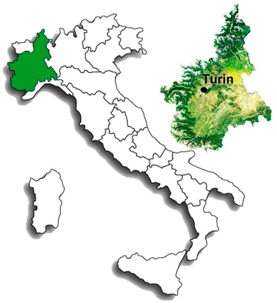
Figure 1.
Localization of the study area in Piedmont (Italy).
This area had a different evolution compared to most of the Western Alps valleys, which have generally an east–west orientation. In fact, the valley under study shows a doubled trend: a first part SSW-NNE trending and a second one E-W trending. The valley in the proximity of the study area has a minimum altitude of around 1000 m a.s.l. and a maximum of around 1550 m a.s.l. From a geological point of view, the area is part of the Pennidic Domain, in the axial portion of the Western Alps, and it is characterized by high-grade metamorphism in addition to the presence of ophiolite masses. In particular, the outcrops of the study area are mainly represented by micaschists with variable petrographic composition that belong to the Dora-Maira Massif. Levels of impure marbles and orthogneisses can be also found in the area, in addition to eluvial–colluvial quaternary deposits, screes, and screes in large blocks (Figure 2).
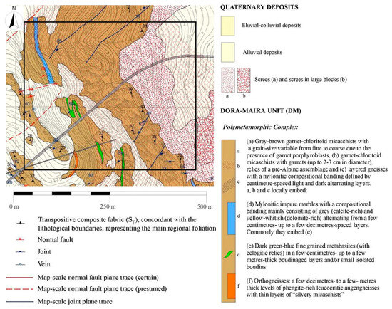
Figure 2.
Geological map of the study area [45]. The study area is indicated by the black rectangle.
The structural setting of the area is the result of four different sin-metamorphic phases during the Alpine orogeny: pre- to syn-collisional D1 and D2 phases and post-collisional D3 and D4 phases. The D1 phase, developed as metamorphic eclogitic facies, is responsible for the development of mineralization levels [46] and mylonitic foliation. The stretching associated with the D1 phase shows a low dipping toward the west [47]. The D2 phase is characterized by the presence of isoclinal folds showing thickened hinges and thin limbs, an N-S sub-horizontal axis, and west-dipping axial planes. The folds and the axial plane foliations appear to have been refolded during the D3 phase, mainly in the western part of the area. The D3 folds developed in the greenschists metamorphic facies and are characterized by crenulation cleavage and open geometries. The axial planes of the D3 structures show a slight NE dipping, with sub-horizontal axes NS trending. The last D4 phase caused the formation of extensional faults following the sin-metamorphic structures. The faults generally show a NE-SW direction, strongly dipping towards the NW. At the regional scale, the faults follow an en-echelon layout with spacing of several hundreds of meters [46,48].
In this context, the valley where the rocky slope under study is located is characterized by an evident asymmetry due to the west-dipping foliation of an isoclinal fold, which causes a different structural setting between the eastern and western slopes (dip slope and anti-dip slope, respectively).
3. Material and Methods
3.1. UAV and Topographic Surveys
Due to the complex morphology of the area, with high and steep slopes, a photogrammetric survey was carried out by using a DJI Mavic 2 Pro UAV, equipped with a digital camera, the Hasselblad L1D-20C, characterized by a 1” sensor size and 20 MP of resolution. An alternative would have involved the use of a TLS or a UAV-mounted LiDAR (Light Detection And Ranging) device, but the absence of proper locations for the multiple TLS scans required and the problems related to the uncertain strength of the GNSS signal, which is essential in UAV-based LiDAR for the direct georeferencing of the point cloud, made the choice of a UAV photogrammetric survey the most advisable. The whole study area (approximately 6 ha) was covered by a total of 5 different flights, 2 with nadiral acquisition and 3 with frontal acquisition, and a flight direction parallel to the rock slope (overlap 75%–sidelap 75%). A total of 990 images, with an average Ground Sample Distance (GSD) of 3.5 cm, were acquired.
In addition to the UAV flights, a topographic survey was carried out to acquire 3D coordinates of specific Ground Control Points (GCPs) to be used for the exterior orientation of the images during the photogrammetric processing. Six out of 17 GCPs were acquired by measuring artificial targets (50 × 50 cm black and yellow panels) placed in accessible zones of the study area, while the rest were acquired by measuring natural features recognizable in the UAV images. The coordinates of natural targets were measured by the combined use of a Total Station (TS—Leica Geosystems™ Nova MS50) and two Global Navigation Satellite System receivers (GNSS—Leica Geosystems™ GS15). The two GNSS devices firstly worked independently, in static positioning, for a period of approximately 3 h; then, the two measured points were processed using Leica Geosystems™ Infinity [49] software and differential methods by combining simultaneous records from a permanent GNSS station of the Leica Geosystems™ SmartNet ItalPos national network (i.e., Gravere/GRAV). This procedure allowed sub-centimetric accuracy for the two GNSS points, later necessary for georeferencing the targets measured during the TS survey, through a spatial transformation procedure (i.e., roto-translation). Differently, the coordinates of the artificial GCPs placed in accessible zones of the study area were acquired by using the two geodetic GNSS receivers (base/rover configuration) working in Real Time Kinematic (RTK) positioning with a minimum acquisition time of 1 min per point at 1 s of observation rate. The orthometric height of all the measured points was later calculated by using ConverGo software [50].
3.2. Photogrammetric Processing
The images acquired during the UAV survey were processed by using AgisoftTM Metashape [51]. The software is based on SfM-MVS technology, which uses advanced image matching algorithms, and it is therefore capable of solving the camera interior and exterior orientation parameters for the creation of georeferenced spatial data as 3D point clouds and derived products (i.e., Digital Surface Models, Digital Terrain Models, and orthophotos).
The first processing phase refers to the image alignment: at this stage, the interior and relative orientation parameters are solved and a 3D sparse cloud is generated. The sparse cloud is composed of tie points extracted without imposing any limit number to improve the final re-projection accuracy. After the alignment step, the exterior orientation parameters were solved by using the GCPs (adopted reference system ETRF2000/UTM32N) and the “optimize” tool of the software, which allows for the adjustment of the estimated camera positions, the correction of non-linear deformations, and the minimization of the re-projection errors. After this, a georeferenced dense 3D point cloud of the whole slope was generated with high quality and moderate depth filtering settings. The generated 3D model was the base for the creation of the digital surface model and the orthophotomosaic of the area. The digital surface model was then manually classified to remove vegetation from the model to obtain a final Digital Terrain Model (DTM). Given the sporadic presence of vegetation and the complete direct control from an expert operator on the classification, the obtained DTM was qualitatively suitable for the next analyses.
3.3. Fracture Pattern Analysis
The 3D dense point cloud obtained from the photogrammetric process was used to study the structural setting of the rock slope by employing the software CloudCompareTM [52]. In fact, thanks to the “Compass” plugin of the software, approximately 1600 discontinuities were measured on the different portions of the slope through the interpolation of a plane on a selection of points chosen by an expert operator; the software then calculated the dip and dip direction of every plane.
Such data were then integrated with the ones directly measured from engineering–geological surveys conducted by the authors in the accessible zones of the area (described in Section 3.4).
Once the discontinuity sets were identified through stereonet analysis, a semi-automatic procedure for the extraction of the discontinuities was realized by using the CloudCompareTM qFacets plugin [53]. In this way, a total of around 56,600 fractures have been identified and localized on the whole slope extension. Such an operation was essential to evaluate the density distribution of every discontinuity set.
The illustrated approach was chosen to increase the reliability of the analysis. To summarize, a manual procedure was firstly realized (combining information derived from deterministic point cloud analysis and a direct engineering–geological survey), where expert operators had complete control on the collected data, avoiding the identification of erroneous discontinuities. Then, the discontinuities automatically searched by the software algorithm were filtered based on the dip, dip direction, and dispersion parameters of the previously manually identified sets. This allowed the collection of a huge number of discontinuities rapidly and with a high degree of reliability.
3.4. Engineering–Geological Survey
Traditional engineering–geological surveys were performed on the safe, accessible zones of the study area (Figure 3) for a direct characterization of the rock mass. Fieldworks allowed for the identification of lithologies and discontinuity characteristics. Therefore, it was possible to collect fundamental information to define the discontinuity properties. In fact, as previously described, the analysis of the point cloud is generally used to measure the geometrical characteristics of the discontinuities (attitude, length, spacing, etc.) but cannot be used for other important properties such as the kind of filling, weathering, Uniaxial Compressive Strength (UCS), and so on. In addition, the manual acquisition of the geometrical properties of the discontinuities is fundamental to compare and validate the remotely sensed data. Hence, information about discontinuity orientation, spacing, persistence, aperture, infilling, roughness, weathering, and UCS (derived from Schmidt hammer rebound values) was collected with traditional techniques directly in the field.
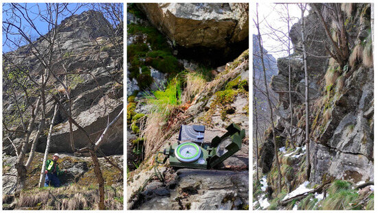
Figure 3.
Some photos taken during the engineering–geological survey.
Despite the importance of a direct approach, the complex morphological conditions of the area, with very steep slopes (with sub-vertical portions) that were mostly inaccessible for safety reasons (i.e., high rockfall risk), made the integration with remotely derived data fundamental for a complete characterization of the rock mass. In fact, without the information obtained from the 3D model, it would have been impossible to collect data sufficient for a very reliable hazard analysis, which would have been done with statistical data and empirical approaches.
All the collected data were analyzed in their completeness for the determination of the discontinuity set characteristics and for the application of the Q-slope approach proposed by Bar and Barton [54].
The Q-slope has been recently introduced for the evaluation of the probability of slope failures and it is based on the traditional Q-system proposed by Barton et al. [55] for underground excavations. The Q-slope allows for the determination of a slope stability condition through the following Equation (1):
where RQD is the Rock Quality Designation Index [56], Jn represents the number of discontinuity sets, Jr refers to the discontinuity roughness, Ja is related to the discontinuity alteration (i.e., weathering), Jwice expresses the geological and environmental conditions, and SRFslope is the Strength Reduction Factor (result of a series of geological and geotechnical conditions). The second factor (Jr/Ja) must be multiplied by the Orientation factor (O), which has been included to consider the relative orientation between discontinuities and slope. The final Q-slope value can then be used, together with the mean dip angle of a rock face, in the Stability Chart (Figure 4) to verify the stability condition of the slope. In addition, specific equations may be used to determine the dip angle of the rock face to meet different PoF conditions (1%, 15%, 30%, 50%; Figure 4).
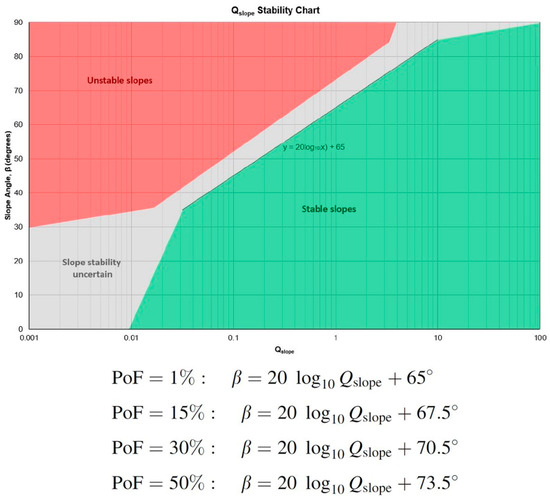
Figure 4.
Q-slope stability graph and PoF equations, modified from [54].
3.5. Kinematic Stability Analysis
The kinematic stability analysis is a basic study that does not consider the dynamic forces that contribute to the equilibrium or the failure of a rock block, but only the dip and dip direction of slope and the discontinuity set’s attitude and friction angle. Nevertheless, it is a common preliminary analysis that allows for the identification of possible unstable blocks or zones. Such analysis is based on the Markland test [57], which represents a stereographic technique for analyzing the possibility of failure of blocks through planar sliding, toppling, and wedge sliding.
It must be specified that, as reported by Brideau and Stead [58], the results of a kinematic analysis are strongly influenced by the topography of the study area. To obtain reliable results, an integrated kinematic–GIS-based approach was adopted in our study. Such an approach cross-checks the result of the kinematic test with a spatial analysis to localize potentially unstable areas, using as input the DTM obtained from the photogrammetric processing at a spatial resolution of 1 m (a good compromise between the need to have a detailed model and a readable output). Therefore, in a GIS environment, by using ESRITM ArcGIS Desktop software [59], information about the dip and dip direction of every DTM cell was obtained by using the tools Slope and Aspect, respectively. To simplify the analysis, the Aspect model was reclassified into 15 classes with a range of 24°, as shown in Table 1.

Table 1.
Classes of Aspect with indication of dip direction range and average values.
Then, for every Aspect class, a kinematic stability analysis was performed by using the RocScienceTM Inc. software Dips [60] to identify the potential for sliding and the limit angle for the instability to occur. The limit angle is an important piece of data since it refers to the steepest safe angle that a rock slope can reach without triggering a rockfall.
At the end, by the combination of the DTM Aspect and Slope data with the information about the discontinuity set orientations and friction angles, it was possible to identify areas on the slopes that may be susceptible to rockfall.
3.6. Dynamic Slope Stability Analysis
The kinematic analysis previously described does not give information about the FS of potentially unstable blocks. For a proper stability analysis, in fact, it is necessary to take into consideration also other static (i.e., block weight) and dynamic (i.e., seismic) forces. In accordance with the Italian regulations, the latter was evaluated following the pseudo-static approach that, for the area under study, is the result of the application of the following coefficients (https://geoapp.eu/parametrisismici2018/ (accessed on 29 January 2022)): Amax (Maximum Acceleration) equal to 2.212 m/s2, Kh (Horizontal Seismic Coefficient) equal to 0.054, and Kv (Vertical Seismic Coefficient) equal to 0.027.
The dynamic slope stability analysis was performed by using the RocScienceTM Inc. software RocPlane (for planar sliding [61]), Swedge (for wedge sliding [62]), and RocTopple (for direct toppling [63]).
Given the geo-mechanical complexity of the area and the variety of possible rockfalls of different size, in addition to the uncertainty on the input data due to the absence of specific laboratory tests, a probabilistic approach was adopted. A probabilistic analysis can be executed by considering a range of values rather than one, following a chosen statistical distribution. The final result is, therefore, a PoF and not a single deterministic FS value. In this context, the adopted probabilistic method was the “Latin Hypercube” [64,65], which gives results comparable to those obtainable from the Monte Carlo technique, but with fewer samples [64,65]. The method is based upon “stratified” sampling with random selection within each stratum, resulting in a smoother sampling of the probability distributions [62].
In this research, every probabilistic simulation was carried out through a total of 10,000 simulations to obtain robust statistical data, considering a target FS of 1.2 to account for a certain degree of uncertainty typical for this kind of analysis. The analyses were performed by adopting the Barton–Bandis criterion [66,67,68,69] according to the following Equation (2):
where is the normal stress acting on the surface, JRC is the Joint Roughness Coefficient, JCS is the Joint Compressive Strength, and is the residual friction angle.
Such a criterion was chosen as an alternative to the widespread Mohr–Coulomb criterion, since it is common knowledge that joints, if not completely closed or infilled, do not offer sliding resistance because of cohesion but only due to a high friction angle [70]. Therefore, the Barton–Bandis criterion neglects the cohesion contribution, focusing on the friction angle, which depends on discontinuity properties measurable in the field, such as roughness and rock mechanical compressive strength.
The dynamic stability analyses were performed for the main rockfall type identified in the kinematic analysis and they observed both the approaches, in static and seismic conditions, for a total of 136 different analyses. The results returned PoF values, which were grouped into four classes: low probability of failure (<10%), medium probability (10% ≤ x < 30%), high probability (30% ≤ x < 50%), and very high probability (>50%).
3.7. Rockfall Hazard Assesment
For the rockfall hazard assessment, a methodology that considers the results of kinematic and dynamic stability analyses, in addition to discontinuity density, was developed and adopted. The in-depth analysis of the discontinuity set’s density distribution was considered essential, since the fracture pattern in a rock mass may be simplified for an easier description but it is hardly homogeneous. Consequently, it is important to map the discontinuity distribution to avoid the classification with the same hazard level of zones with very different fracture density.
From a methodological point of view, a shapefile containing the barycenter of the fractures that were identified in CloudCompareTM through the semi-automatic procedures was imported into the GIS environment (ArcGIS Desktop software [59]). Then, the Point Density function [71] was used to define the spatial density distribution of every joint set. The function calculates the density of point features around each output raster cell. Practically, a neighborhood is defined around each raster cell center, and the number of points that fall within the neighborhood is summed and divided by the area of the neighborhood [72]. In this work, the density value of each cell (0.5 m size) was calculated by using a circular shape with 15 m radius. The choice of such a radius was obtained after a careful process of data calibration and several attempts to find the best compromise between detail and representativeness at the work scale.
Subsequently, thresholds were defined to identify three density classes: low density (<15), medium density (15 ≤ x < 50), and high density (≥50). Then, it was possible to cross-check data (through simple GIS queries) about GIS-based kinematic analysis (indicating where the geometrical condition for a possible rockfall exists) and the density distribution of discontinuity sets to obtain a final rockfall hazard map where areas at low, medium, and high level are identified. In other words, the hazard of a given zone can be classified as high if the geometrical conditions for instability are present (from the kinematic analysis) only if the density of the discontinuity is high. Differently, if an area exhibits the geometrical conditions for a possible rockfall, but it shows low discontinuity density, then the area would not be classified as hazardous. The map is generic in respect to the rockfall type and, even if created by analyzing separately planar sliding, wedge sliding, and toppling, it considers the hazard for all the possible failures. This map was called the Level 1 hazard map since it can be useful to localize possible block source areas, but it does not describe the hazard level, omitting the PoF. For this reason, a Level 2 hazard map was proposed by cross-checking the Level 1 hazard map and the PoF of every possible rockfall type resulting from the dynamic stability analysis. To do this, a specific function was created in the GIS environment to consider all the possible combinations of rockfall type, the discontinuity set’s density distribution, and PoFs, for more than 850 possible combinations. At the end, two different hazard maps were created, respectively, for static and dynamic conditions. The Level 2 hazard maps partition the whole slope into three hazard rockfall levels: low, medium, and high. Table 2 shows the matrix used for the final hazard classification.
Table 2.
Matrix and criteria used for the identification of the Level 2 rockfall hazard (1—Low, 2—Medium, 3—High).
In Figure 5, the flowchart that summarizes the entire work process is shown.
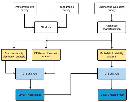
Figure 5.
Flowchart of the proposed rockfall hazard assessment.
4. Results
4.1. 3D Model
The post-processing of the topographic data was performed using Leica Geosys-tems™ Infinity and ConveRgo software and permitted us to obtain 3D coordinates (ETRF2000/UTM32N reference system) of GCPs with a sufficient accuracy level. The accuracy of the two GNSS points measured in static positioning for a period of around 3 h resulted in an RMSE of 3 mm in the horizontal plane and 6 mm in altimetry. The coordinates of artificial targets measured on the ground in RTK have a horizontal accuracy of 1 cm and a vertical accuracy of 1.2 cm. The GCPs measured by the TS on the rock slope show a precision of 3 mm even if it must be underlined that neither artificial targets nor prisms were placed on the versant, where their collimation can involve some uncertainty.
As already noted in Section 3.1, the survey of GCPs on the slopes uses the coordinates of the two GNSS points to apply a spatial transformation procedure (i.e., roto-translation) from the local TS system to the ETRF2000/UTM32N reference system. The average error calculated from the adjustment of TS and GNSS data is 3.8 cm, with a confidence σ1 of ±0.11 and σ2 of ±0.23.
The photogrammetric process was conducted by using 14 GCPs and 3 Check Points (CPs) with a final Root Mean Square Error (RMSE) of 16 cm. Given the complexity and the extent of the area, and the low GNSS coverage, the RMSE was considered adequate for the rest of the analysis.
The final dense point cloud, which is shown in Figure 6, is composed of approximately 103 million points. A 10 cm digital surface model was generated from the photogrammetric point cloud. Such a model was then used to create the orthophotomosaics of the area (frontal and nadiral) with a resolution of 4 cm/pixel (an example is given in Figure 7). As already mentioned, the point cloud was also cleaned of vegetation to create the DTM of the rock slope.
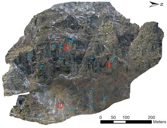
Figure 6.
Prospective view of the georeferenced 3D point cloud; the blue flags localize GCPs and CPs on the slopes; CPs are highlighted by a red circle.
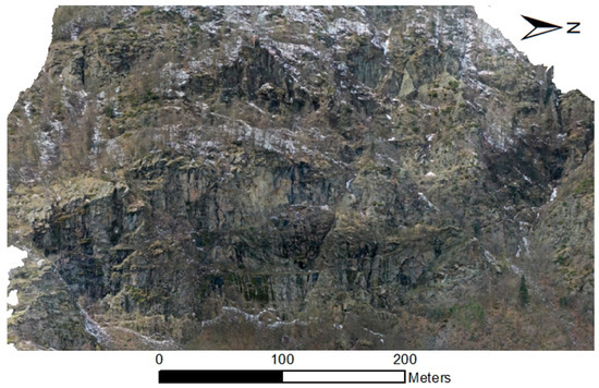
Figure 7.
Example of the orthophotomosaic in frontal view.
4.2. Rockfall Hazard Assesment
4.2.1. Rock Mass Engineering–Geological Characterization
The engineering–geological field survey confirmed that the majority of the rock slope is composed of micaschists, with a localized level of impure marbles. The grey–brown micaschists show a variable grain size from fine to coarse. The presence of quartz is often notable and sometimes concentrated in pluricentimetric-thick veins. From a geotechnical point of view, the UCS measured with the Schmidt hammer is approximately 120 MPa, even if the anisotropic nature of the rock implies a significant difference in strength when the load is applied in different directions. Analyses of the collected data allowed for a clear understanding of the structural and geo-mechanical setting of the study area. This was possible thanks to the high number of deterministically measured discontinuities that were collected from the 3D model and their integration with data measured in the field through traditional techniques. Such integration allowed for the validation of the remotely acquired data and the identification of the main discontinuity sets and their variability. Figure 8 shows the final stereographic projection with seven discontinuity sets highlighted. The characteristics of every set are shown in Table 3, which includes the dispersion coefficient Fisher K (the lower the K coefficient, the greater the discontinuity set dispersion).
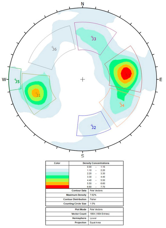
Figure 8.
Equal area projection of the pole of the discontinuities on a stereonet (Schmidt, equal area, lower hemisphere). The data come from both engineering–geological surveys and 3D point cloud processing.
Table 3.
Geo-mechanical characteristics of the different discontinuity sets; J = joint, S = schistosity.
The geo-mechanical condition of the rock mass was then evaluated through the Q-slope classification (Table 4), which provided a final value of 0.71.
Table 4.
Rock mass classification through Q-slope method.
Considering an average dip of the slope of 70°, the application of the stability graph (Figure 4) indicates a potential unstable condition for the rock slope under study, with possible development of rockfall events. This is mainly due to the presence of evident planar and wedge sliding. In addition, Table 5 shows the results of the application of Figure 4’s equations used for evaluating the maximum slope angle of the rock face necessary (in the absence of precautionary measures) to obtain a PoF of 1, 15, 30, and 50%, respectively.
Table 5.
Dip angle values of the rockface necessary to obtain PoF equal to 1, 15, 30, and 50%, respectively, according to the Q-slope method [54].
4.2.2. Kinematic Stability Analysis
The kinematic analysis was performed by assuming a friction angle equal to 30°. In the absence of specific laboratory tests, such a value was chosen after a series of different considerations. In the Q-system method [55], the authors proposed a friction angle for every Ja class. In this study, the Ja value ranges from 1 to 2, which is equivalent to a residual friction angle between 25 and 35 degrees. In addition, Barton and Choubey [67] proposed a basic friction angle between 25 and 30 degrees for metamorphic rock joints. Starting from such value, it is then possible to calculate the residual friction angle of the discontinuities by using the following Equation (3) proposed by Barton and Choubey [67]:
where is the residual friction angle, is the basic friction angle, r is the Schmidt hammer rebound value on the discontinuity surface, and R is the Schmidt hammer rebound value on unweathered surfaces. By the application of Equation (3), values between 20° and 25° are obtained. As regards the estimate of the peak friction angle (), reference was made to the following Equation (4) proposed by Barton [73]:
Results from the application of Equation (4) indicate a between 36° and 45°. Consequently, considering that, for block failure analyses, it is reasonable to use the , the choice of using a value of 30° for the discontinuities appears realistic and precautionary.
The results of the kinematic analysis for planar sliding, wedge sliding, and direct toppling are summarized in Table 6, Table 7 and Table 8; the tables show, for every possible slope dip direction, the discontinuity sets that may lead to a falling block and the associated slope limit angle.
Table 6.
Kinematic stability analysis results: planar sliding.
Table 7.
Kinematic stability analysis results: wedge sliding.
Table 8.
Kinematic stability analysis results: direct toppling.
4.2.3. Probabilistic Dynamic Stability Analysis
Table 9, Table 10, Table 11, Table 12, Table 13 and Table 14 show the main used parameters (with indication of the Standard Deviation SD; normal distribution or, in a few cases, truncated normal distribution) and the results of the probabilistic stability analysis (static and seismic conditions). For practical reasons, only the results of the analysis that returned a final PoF higher than 5% are shown. The adopted unit weight of the material (i.e., micaschist) was set equal to 2.5 t/m3.
Table 9.
Probabilistic stability analysis results for planar sliding: J1, J2, and J3 sets.
Table 10.
Probabilistic stability analysis results for planar sliding: J4, J5, and J6 sets.
Table 11.
Probabilistic stability analysis results for wedge sliding.
Table 12.
Probabilistic stability analysis results for wedge sliding.
Table 13.
Probabilistic stability analysis results for direct toppling.
Table 14.
Probabilistic stability analysis results for direct toppling.
Results indicate that the most critical instability is due to planar sliding and direct toppling, while wedge sliding has, on average, lower PoFs.
4.2.4. Rockfall Hazard Maps
The first step for the hazard assessment of the area was the combination of the kinematic stability analysis results with the discontinuity density maps. These are basically deterministic maps that identify the density of the different discontinuity sets on the rock slope. The maps were obtained from the semi-automatic procedure described in Section 3.7 and are shown in Figure 9.
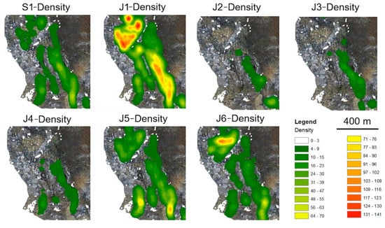
Figure 9.
Orthophotos of the study area with indication of fracture density distribution for every identified discontinuity set.
As previously described, three different joint density classes were defined: low density (<15), medium density (15 ≤ x < 50), and high density (≥50). This information, together with the dip and dip direction of the rock slope, was included in a single raster and then used to create, through an SQL expression selecting the areas characterized by different combinations of rockfall type, the Level 1 hazard map (Figure 10) at a spatial resolution of 1 m.
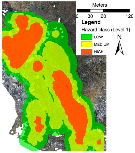
Figure 10.
Level 1 hazard map. Orthophoto of the study area with identification of zones at different levels of hazard.
The Level 1 hazard map highlights a generic potential instability of the rock slope, with large areas characterized by medium or high fracture density and orientation of the rock slopes unfavorable to stability. Nevertheless, the Level 1 hazard map does not consider the PoF of the different conditions. In fact, an area with a high Level 1 hazard could be characterized by low PoF, reducing the final rockfall hazard level.
Therefore, since this topic is fundamental and must be considered, a new map, called the Level 2 hazard map, was calculated. The information referring to the different stability analyses was combined in the raster describing the dip and dip direction of the slope and fracture density data, and a new SQL expression was created to take into consideration all the possible combinations of Level 1 hazard and PoFs. Every pixel of the rock face was investigated to identify its geometrical conditions favorable or not to instability (from kinematic analyses), its fracture density, and its PoF. According to the conditions shown in Table 2, the rockfall hazard level of every pixel was classified as high, medium, or low. Figure 11 (static condition) and Figure 12 (seismic condition) show the frontal view of the final Level 2 hazard maps.
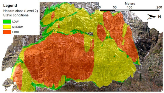
Figure 11.
Frontal view of the Level 2 hazard map (static conditions).
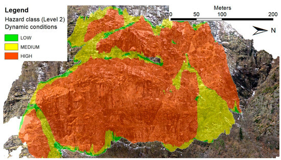
Figure 12.
Frontal view of the Level 2 hazard map (seismic conditions).
5. Discussion
The engineering–geological characterization of the studied rock slope highlighted some critical issues, especially where the rock face slope angle is higher than 60°. This condition can pose some instability troubles, also in relation to the unfavorable orientation of some discontinuity sets, that can cause potential block failures. The Q-slope classification method confirms the possibility of instability problems well-fitting with field observations when numerous sliding planes residual of past sliding events and many rock blocks at the base of the slope were observed.
Such indications are undoubtedly useful and can be obtained by traditional techniques based on statistical approaches and empirical methods. Nevertheless, a more precise and deterministic analysis can be essential in certain cases—for example, when large areas are analyzed and there is the necessity to prioritize the remediation measures in the most dangerous zones. To achieve this aim, the in-depth analysis of the fracture pattern is essential, especially if implemented with the characterization of the discontinuity densities. In a natural rock slope, in fact, the fracture pattern is often variable; therefore, a deterministic mapping of the discontinuities is crucial to determine the fracture sets and their density distribution all over the slopes. Even though the discontinuity pattern is fundamental for rock instability investigations, the concept of fracture density is rarely considered as it ought to be in hazard assessment procedures, thus neglecting the contribution of local discontinuities and their orientation on instability. For this reason, in this paper, a procedure for including in hazard assessment procedures detailed fracture density maps was adopted. This was achieved thanks to an in-depth analysis of a 3D point cloud obtained from UAV-based photogrammetry. With the aim of increasing the reliability of the analysis, the main discontinuity sets were identified on the point cloud by an expert operator through the manual deterministic acquisition of many fracture planes. In this way, the control of the collected data was complete, avoiding the identification of erroneous discontinuities. Thanks to the produced fracture patterns, an automatic procedure for the automatic identification of discontinuities on the slope was run through a specific algorithm. This allowed the recognition of more than 56,000 discontinuities, crucial for the deterministic identification of the density distribution of every single set. The reliability of these data was guaranteed by consistency with the distribution of the discontinuity attitudes measured during the engineering–geological survey. A deterministic map of the fracture density is essential for an accurate and detailed hazard assessment since the traditional stability analysis can only indicate the possible presence of a failure mechanism (which can be triggered if certain conditions occur), and it does not permit the localization of areas with different hazard levels. In this context, in fact, an area with a higher fracture density (with other stability factors being equal) will have a higher rockfall probability compared to another with a lower fracture density. Given the variability that generally marks a fracture pattern of a rock mass, it is also possible that a specific discontinuity set is not present in a certain portion of a rock slope, reducing the hazard practically to zero. In this work, the fracture density map was used to create a Level 1 hazard map.
Such a map clearly indicates where a possible unstable block is more likely to be localized. Nevertheless, to understand the real level of hazard for the different zones of the slope, it was also necessary to perform an additional dynamic stability analysis to calculate the PoF for every kind of possible rockfall (planar sliding, wedge sliding, and direct toppling). The PoF was then used to create the Level 2 hazard map, which clearly indicates areas where a rockfall event is more likely to occur, since it uses the fracture density, the geometric conditions (dip and dip directions of slope and joints), and the PoF.
The maps produced in this work have a spatial resolution of 1 m, but this can be changed on a case-by-case basis.
The obtained results show good correspondence with field observations, where the major signs of rockfall events are clearly visible at the base of the slope classified as high hazard in the Level 2 hazard map. In Figure 13, the vegetation is present on the natural deposit below zones at a medium–low hazard level (static conditions); moreover, under high-hazard zones, it is practically absent, confirming the higher frequency of rockfall events.
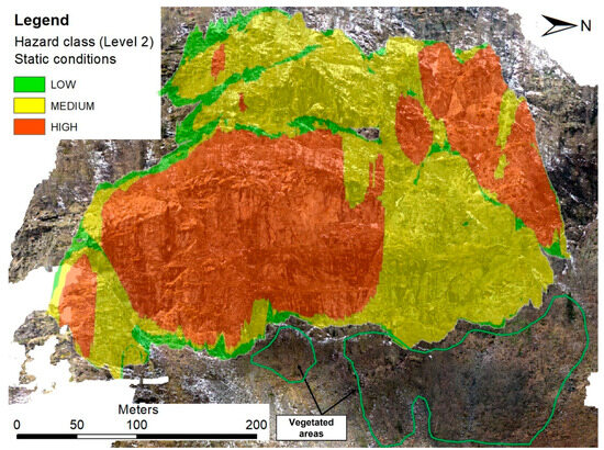
Figure 13.
Level 2 hazard map, static conditions, with indication of the areas covered by vegetation.
The proposed innovative approach allows the realization of a deterministic rockfall hazard map that considers the multiple data to be considered when facing a rockfall instability study. Every factor is weighted and integrated with the others, giving the possibility to identify the most dangerous areas in which to prioritize remediation works. The approach used in this research was conducted by standard techniques well-known to the geoscientist community and does not consider the use of ML algorithms, which could be a future direction of the work.
6. Conclusions
In this paper, an approach that considers results from kinematic analysis, fracture density maps, and failure probability was used, and related hazard maps, indicating where to prioritize remediation measures, were created. Seven discontinuity sets were identified on a natural rock slope through the analyses of field (engineering–geological survey) and 3D UAV-based photogrammetry data. A semi-automatic procedure was then used to identify approximately 56,600 discontinuities on the rock slope. Such deterministic mapping was used to create seven fracture density maps that were combined in a GIS environment with the results of kinematic and dynamic stability analyses performed with a probabilistic approach. The final output was a hazard map that classifies the rock slope according to the combination of three hazard factors: kinematic predisposition to rockfall (planar sliding, wedge sliding, direct toppling), fracture density, and probability of failure.
The main advantages of the illustrated approach can be summarized as follows:
- Methodology based on GIS spatial analysis, which allows hazard assessment of slopes prone to rockfall events, localizing the higher-risk areas in a punctual way. The approach is accurate and does not require complex algorithms to be applied.
- The approach is not time-consuming compared to other approaches, but it requires the direct control of an operator for all the steps of the analysis.
- Semi-automatic procedure for the in-depth study of the fracture pattern, which allows for a complete and deterministic rock mass characterization and for the realization of detailed fracture density maps.
- Creation of reliable hazard maps based on the main three factors that contribute to rockfall instability (kinematic predisposition to rockfall, fracture density distribution, probability of failure).
- Improved rockfall prediction, with detailed, scalable, and accurate hazard maps that allow for the localization of areas in which to prioritize future remediation works.
Author Contributions
Conceptualization: C.V. and R.S.; methodology, C.V. and R.S.; formal analysis, C.V.; investigation, C.V. and A.R.; writing—original draft preparation, C.V.; writing—review and editing, C.V. and R.S.; supervision, R.S. All authors have read and agreed to the published version of the manuscript.
Funding
This research received no external funding.
Institutional Review Board Statement
Not applicable.
Informed Consent Statement
Not applicable.
Data Availability Statement
The data presented in this study are available upon request to be sent to the corresponding author. The data are not publicly available due to privacy restrictions.
Conflicts of Interest
The authors declare no conflict of interest.
References
- Vanneschi, C.; Eyre, M.; Francioni, M.; Coggan, J. The Use of Remote Sensing Techniques for Monitoring and Characterization of Slope Instability. Proc. Eng. 2017, 191, 150–157. [Google Scholar] [CrossRef]
- Francioni, M.; Salvini, R.; Stead, D.; Coggan, J. Improvements in the integration of remote sensing and rock slope modelling. Nat. Hazards 2017, 90, 975–1004. [Google Scholar] [CrossRef]
- Robiati, C.; Eyre, M.; Vanneschi, C.; Francioni, M.; Venn, A.; Coggan, J. Application of Remote Sensing Data for Evaluation of Rockfall Potential within a Quarry Slope. ISPRS Int. J. Geo-Inf. 2019, 8, 367. [Google Scholar] [CrossRef]
- Vanneschi, C.; Eyre, M.; Burda, J.; Žižka, L.; Francioni, M.; Coggan, J.S. Investigation of landslide failure mechanisms adjacent to lignite mining operations in North Bohemia (Czech Republic) through a limit equilibrium/finite element modelling approach. Geomorphology 2018, 320, 142–153. [Google Scholar] [CrossRef]
- Vanneschi, C.; Eyre, M.; Venn, A.; Coggan, J.S. Investigation and modeling of direct toppling using a three-dimensional distinct element approach with incorporation of point cloud geometry. Landslides 2019, 16, 1453–1465. [Google Scholar] [CrossRef]
- Assali, P.; Grussenmeyer, P.; Villemin, T.; Pollet, N.; Viguier, F. Surveying and modeling of rock discontinuities by terrestrial laser scanning and photogrammetry: Semi-automatic approaches for linear outcrop inspection. J. Struct. Geol. 2014, 66, 102–114. [Google Scholar] [CrossRef]
- Singh, S.K.; Raval, S.; Banerjee, B.P. Automated structural discontinuity mapping in a rock face occluded by vegetation using mobile laser scanning. Eng. Geol. 2021, 285, 106040. [Google Scholar] [CrossRef]
- Idrees, M.O.; Pradhan, B. Geostructural stability assessment of cave using rock surface discontinuity extracted from terrestrial laser scanning point cloud. J. Rock Mech. Geotech. Eng. 2018, 10, 534–544. [Google Scholar] [CrossRef]
- Fekete, S.; Diederichs, M. Integration of three-dimensional laser scanning with discontinuum modelling for stability analysis of tunnels in blocky rockmasses. Int. J. Rock Mech. Min. Sci. 2013, 57, 11–23. [Google Scholar] [CrossRef]
- Mastrorocco, G.; Salvini, R.; Vanneschi, C. Fracture mapping in challenging environment: A 3D virtual reality approach combining terrestrial LiDAR and high definition images. Bull. Eng. Geol. Environ. 2017, 77, 691–707. [Google Scholar] [CrossRef]
- Spetsakis, M.; Aloimonos, J.Y. A multi-frame approach to visual motion perception. Int. J. Comput. Vis. 1991, 6, 245–255. [Google Scholar] [CrossRef]
- Westoby, M.J.; Brasington, J.; Glasser, N.F.; Hambrey, M.J.; Reynolds, J.M. “Structure-from-Motion” photogrammetry: A low-cost, effective tool for geoscience applications. Geomorphology 2012, 179, 300–314. [Google Scholar] [CrossRef]
- Fonstad, M.A.; Dietrich, J.T.; Courville, B.C.; Jensen, J.L.; Carbonneau, P.E. Topographic structure from motion: A new development in photogrammetric measurement. Earth Surf. Process. Landforms 2013, 38, 421–430. [Google Scholar] [CrossRef]
- Colomina, I.; Molina, P. Unmanned aerial systems for photogrammetry and remote sensing: A review. ISPRS J. Photogramm. Remote Sens. 2014, 92, 79–97. [Google Scholar] [CrossRef]
- Giordan, D.; Adams, M.S.; Aicardi, I.; Alicandro, M.; Allasia, P.; Baldo, M.; De Berardinis, P.; Dominici, D.; Godone, D.; Hobbs, P.; et al. The use of unmanned aerial vehicles (UAVs) for engineering geology applications. Bull. Eng. Geol. Environ. 2020, 79, 3437–3481. [Google Scholar] [CrossRef]
- O’Banion, M.S.; Olsen, M.J.; Rault, C.; Wartman, J.; Cunningham, K. Suitability of structure from motion for rock-slope assessment. Photogramm. Rec. 2018, 33, 217–242. [Google Scholar] [CrossRef]
- Gallup, D.; Frahm, J.M.; Mordohai, P.; Yang, Q.; Pollefeys, M. Real-time plane-sweeping stereo with multiple sweeping directions. In Proceedings of the IEEE Computer Society Conference on Computer Vision and Pattern Recognition, Minneapolis, MN, USA, 17–22 June 2007; p. 9. [Google Scholar]
- Goesele, M.; Snavely, N.; Curless, B.; Hoppe, H.; Seitz, S.M. Multi-view stereo for community photo collections. In Proceedings of the IEEE International Conference on Computer Vision, Rio de Janeiro, Brazil, 14–21 October 2007; p. 8. [Google Scholar]
- Jancosek, M.; Shekhovtsov, A.; Pajdla, T. Scalable multiview stereo. In Proceedings of the IEEE Workshop on 3D Digital Imaging and Modeling, Kyoto, Japan, 27 September–4 October 2009; p. 8. [Google Scholar]
- Sturzenegger, M.; Stead, D. Close-range terrestrial digital photogrammetry and terrestrial laser scanning for discontinuity characterization on rock cuts. Eng. Geol. 2009, 106, 163–182. [Google Scholar] [CrossRef]
- Lato, M.J.; Vöge, M. Automated mapping of rock discontinuities in 3D lidar and photogrammetry models. Int. J. Rock Mech. Min. Sci. 2012, 54, 150–158. [Google Scholar] [CrossRef]
- Manousakis, J.; Zekkos, D.; Saroglou, F.; Clark, M. Comparison of UAV-enabled photogrammetry-based 3D point clouds and interpolated DSMs of sloping terrain for rockfall hazard analysis. Int. Arch. Photogramm. Remote Sens. Spat. Inf. Sci. 2016, XLII-2/W2, 71–77. [Google Scholar] [CrossRef]
- Wilkinson, M.W.W.; Jones, R.R.R.; Woods, C.E.E.; Gilment, S.R.R.; McCaffrey, K.J.W.J.W.; Kokkalas, S.; Long, J.J.J. A comparison of terrestrial laser scanning and structure-from-motion photogrammetry as methods for digital outcrop acquisition. Geosphere 2016, 12, 1865–1880. [Google Scholar] [CrossRef]
- Kong, D.; Saroglou, C.; Wu, F.; Sha, P.; Li, B. Development and application of UAV-SfM photogrammetry for quantitative characterization of rock mass discontinuities. Int. J. Rock Mech. Min. Sci. 2021, 141, 104729. [Google Scholar] [CrossRef]
- Tziavou, O.; Pytharouli, S.; Souter, J. Unmanned Aerial Vehicle (UAV) based mapping in engineering geological surveys: Considerations for optimum results. Eng. Geol. 2018, 232, 12–21. [Google Scholar] [CrossRef]
- Gilham, J.; Barlow, J.; Moore, R. Detection and analysis of mass wasting events in chalk sea cliffs using UAV photogrammetry. Eng. Geol. 2019, 250, 101–112. [Google Scholar] [CrossRef]
- Haneberg, W.C. Using close range terrestrial digital photogrammetry for 3-D rock slope modeling and discontinuity mapping in the United States. Bull. Eng. Geol. Environ. 2008, 67, 457–469. [Google Scholar] [CrossRef]
- Salvini, R.; Mastrorocco, G.; Esposito, G.; Di Bartolo, S.; Coggan, J.; Vanneschi, C. Use of a remotely piloted aircraft system for hazard assessment in a rocky mining area (Lucca, Italy). Nat. Hazards Earth Syst. Sci. 2018, 18, 287–302. [Google Scholar] [CrossRef]
- Riquelme, A.; Cano, M.; Tomás, R.; Abellán, A. Identification of Rock Slope Discontinuity Sets from Laser Scanner and Photogrammetric Point Clouds: A Comparative Analysis. Proc. Eng. 2017, 191, 838–845. [Google Scholar] [CrossRef]
- Chen, J.; Zhu, H.; Li, X. Automatic extraction of discontinuity orientation from rock mass surface 3D point cloud. Comput. Geosci. 2016, 95, 18–31. [Google Scholar] [CrossRef]
- Zhang, P.; Li, J.; Yang, X.; Zhu, H. Semi-automatic extraction of rock discontinuities from point clouds using the ISODATA clustering algorithm and deviation from mean elevation. Int. J. Rock Mech. Min. Sci. 2018, 110, 76–87. [Google Scholar] [CrossRef]
- Salvini, R.; Vanneschi, C.; Coggan, J.S.; Mastrorocco, G. Evaluation of the Use of UAV Photogrammetry for Rock Discontinuity Roughness Characterization. Rock Mech. Rock Eng. 2020, 53, 3699–3720. [Google Scholar] [CrossRef]
- Li, X.; Chen, Z.; Chen, J.; Zhu, H. Automatic characterization of rock mass discontinuities using 3D point clouds. Eng. Geol. 2019, 259, 105131. [Google Scholar] [CrossRef]
- Ünlüsoy, D.; Süzen, M.L. A new method for automated estimation of joint roughness coefficient for 2D surface profiles using power spectral density. Int. J. Rock Mech. Min. Sci. 2020, 125, 104156. [Google Scholar] [CrossRef]
- Francioni, M.; Salvini, R.; Stead, D.; Giovannini, R.; Riccucci, S.; Vanneschi, C.; Gull, D. An integrated remote sensing-GIS approach for the analysis of an open pit in the Carrara marble district, Italy: Slope stability assessment through kinematic and numerical methods. Comput. Geotech. 2015, 67. [Google Scholar] [CrossRef]
- Park, H.-J.; Lee, J.-H.; Kim, K.-M.; Um, J.-G. Assessment of rock slope stability using GIS-based probabilistic kinematic analysis. Eng. Geol. 2016, 203, 56–69. [Google Scholar] [CrossRef]
- He, L.; Coggan, J.; Francioni, M.; Eyre, M. Maximizing Impacts of Remote Sensing Surveys in Slope Stability—A Novel Method to Incorporate Discontinuities into Machine Learning Landslide Prediction. ISPRS Int. J. Geo-Inf. 2021, 10, 232. [Google Scholar] [CrossRef]
- Jaboyedoff, M.; Baillifard, F.; Philippossian, F.; Rouiller, J.-D. Assessing fracture occurrence using the “weighted fracturing density”: A step towards estimating rock instability hazard. Nat. Hazards Earth Syst. Sci. 2004, 4, 83–93. [Google Scholar] [CrossRef]
- Duncan, J.M. State of the Art: Limit Equilibrium and Finite-Element Analysis of Slopes. J. Geotech. Eng. 1996, 122, 577–596. [Google Scholar] [CrossRef]
- Jiang, S.H.; Huang, J.; Yao, C.; Yang, J. Quantitative risk assessment of slope failure in 2-D spatially variable soils by limit equilibrium method. Appl. Math. Model. 2017, 47, 710–725. [Google Scholar] [CrossRef]
- Liu, T.; Ding, L.; Meng, F.; Li, X.; Zheng, Y. Stability analysis of anti-dip bedding rock slopes using a limit equilibrium model combined with bi-directional evolutionary structural optimization (BESO) method. Comput. Geotech. 2021, 134, 104116. [Google Scholar] [CrossRef]
- Deng, D. Limit equilibrium solution for the rock slope stability under the coupling effect of the shear dilatancy and strain softening. Int. J. Rock Mech. Min. Sci. 2020, 134, 104421. [Google Scholar] [CrossRef]
- Griffiths, D.V.; Lane, P.A. Slope stability analysis by finite elements. Geotechnique 1999, 49, 387–403. [Google Scholar] [CrossRef]
- Park, H.-J.; West, T.R.; Woo, I. Probabilistic analysis of rock slope stability and random properties of discontinuity parameters, Interstate Highway 40, Western North Carolina, USA. Eng. Geol. 2005, 79, 230–250. [Google Scholar] [CrossRef]
- Camanni, G. Geological-Structural Analysis and 3D Modelling of the Fontane Talc Mineralization (Germanasca Valley, Inner Cottian Alps); University of Turin: Turin, Italy, 2010. [Google Scholar]
- Damiano, A. Studio Geologico delle Mineralizzazioni a Talco Nelle Valli Germanasca, Chisone e Pellice (Massiccio Dora-Maira, Alpi Cozie); University of Turin: Turin, Italy, 1997. [Google Scholar]
- Borghi, A.; Sandrone, R. Structural and metamorphic constraints to the evolution of a NW sector of the Dora-Maira Massif (Western Alps). Boll. Soc. Geol. It. 1992, 45, 135–141. [Google Scholar]
- Cadoppi, P.; Camanni, G.; Balestro, G.; Perrone, G. Geology of the Fontane talc mineralization (Germanasca valley, Italian Western Alps). J. Maps 2016, 12, 1170–1177. [Google Scholar] [CrossRef]
- Leica Geosystems AG. Leica Infinity, Version 3.4.2. Leica Geosystems AG—Part of Hexagon. 2021. Available online: https://leica-geosystems.com/products/gnss-systems/software/leica-infinity(accessed on 29 January 2022).
- CISIS. ConveRgo, Version 2.04; CISIS: Roma, Italy, 2012. Available online: https://www.cisis.it/?page_id=3214(accessed on 29 January 2022).
- Agisoft LLC. Agisoft Metashape Professional, Version 1.7.1; Agisoft LLC: St. Petersburg, Russia, 2021. Available online: https://www.agisoft.com/(accessed on 29 January 2022).
- GPL Software. CloudCompare, Version 2. 2021. Available online: http://www.cloudcompare.org/(accessed on 29 January 2022).
- Dewez, T.J.B.; Girardeau-Montaut, D.; Allanic, C.; Rohmer, J. Facets: A Cloudcompare Plugin to Extract Geological Planes from Unstructured 3d Point Clouds. Int. Arch. Photogramm. Remote Sens. Spatial Inf. Sci. 2016, XLI-B5, 799–804. [Google Scholar] [CrossRef]
- Bar, N.; Barton, N. The Q-Slope Method for Rock Slope Engineering. Rock Mech. Rock Eng. 2017, 50, 3307–3322. [Google Scholar] [CrossRef]
- Barton, N.; Lien, R.; Lunde, J. Engineering classification of rock masses for the design of tunnel support. Rock Mech. Felsmechanik Mécanique Roches 1974, 6, 189–239. [Google Scholar] [CrossRef]
- Deere, D.U.; Hendron, A.J.; Patton, F.D.; Cording, E.J. Design of Surface and Near-Surface Construction in Rock. In Proceedings of the 8th U.S. Symposium on Rock Mechanics (USRMS), Minneapolis, MN, USA, 15–17 September 1966; Society of Mining Engineers, American Institute of Mining, Metallurgical and Petroleum Engineers: Minneapolis, MN, USA, 1966; pp. 237–302. [Google Scholar]
- Markland, J.T. A Useful Technique for Estimating the Stability of Rock Slopes When the Rigid Wedge Sliding Type of Failure is Expected; Tylers Green, H.W., Ed.; Imperial College of Science and Technology: London, UK, 1972; Volume 19. [Google Scholar]
- Brideau, M.A.; Stead, D. Evaluating Kinematic Controls on Planar Translational Slope Failure Mechanisms Using Three-Dimensional Distinct Element Modelling. Geotech. Geol. Eng. 2012, 30, 991–1011. [Google Scholar] [CrossRef]
- ESRI. ArcGIS, Version 10.8; ESRI: West Redlands, CA, USA, 2021.
- RocScience Inc. Dips, Graphical and Statistical Analysis of Orientation Data, Version 8; RocScience Inc.: Toronto, ON, Canada, 2021.
- RocScience Inc. RocPlane, Planar Wedge Analysis for Slopes, Version 4; RocScience Inc.: Toronto, ON, Canada, 2021.
- RocScience Inc. SWedge, Surface Wedge Analysis for Slopes, Version 7; RocScience Inc.: Toronto, ON, Canada, 2021.
- RocScience Inc. RocTopple, Toppling Stability Analysis for Slopes, Version 2; RocScience Inc.: Toronto, ON, Canada, 2021.
- Iman, R.L.; Davenport, J.M.; Zeigler, D.K. Latin Hypercube Sampling (a Program User’s Guide); Sandia Labs: Albuquerque, NM, USA, 1980.
- Startzman, R.A. An Improved Computation Procedure for Risk Analysis Problems with Unusual Probability Functions. In Proceedings of the SPE Hydrocarbon Economics and Evaluation Symposium, Dallas, TX, USA, 9–10 March 1989; Society of Petroleum Engineers: Dallas, TX, USA, 1985. [Google Scholar]
- Barton, N. Review of a new shear-strength criterion for rock joints. Eng. Geol. 1973, 7, 287–332. [Google Scholar] [CrossRef]
- Barton, N.; Choubey, V. The shear strength of rock joints in theory and practice. Rock Mech. Felsmechanik Mec. Roches 1977, 10, 1–54. [Google Scholar] [CrossRef]
- Barton, N.R.; Bandis, S.C. Review of predictive capabilities of JRC-JCS model in engineering practice. In Proceedings of the International Symposium on Rock Joints, Leon, Norway, 4–6 June 1990; pp. 603–610. [Google Scholar]
- Barton, N. The shear strength of rock and rock joints. Int. J. Rock Mech. Min. Sci. Geomech. Abstr. 1976, 13, 255–279. [Google Scholar] [CrossRef]
- Barton, N. Shear strength criteria for rock, rock joints, rockfill and rock masses: Problems and some solutions. J. Rock Mech. Geotech. Eng. 2013, 5, 249–261. [Google Scholar] [CrossRef]
- Silverman, B.W. Density Estimation for Statistics and Data Analysis; Routledge: London, UK, 2018; ISBN 9781315140919. [Google Scholar]
- ESRI. ArcGIS PRO, Version 2.9; ESRI: West Redlands, CA, USA, 2021.
- Barton, N. Some new Q-value correlations to assist in site characterisation and tunnel design. Int. J. Rock Mech. Min. Sci. 2002, 39, 185–216. [Google Scholar] [CrossRef]
Publisher’s Note: MDPI stays neutral with regard to jurisdictional claims in published maps and institutional affiliations. |
© 2022 by the authors. Licensee MDPI, Basel, Switzerland. This article is an open access article distributed under the terms and conditions of the Creative Commons Attribution (CC BY) license (https://creativecommons.org/licenses/by/4.0/).