Article

Aerial Imagery Can Detect Nitrogen Fertilizer Effects on Biomass and Stand Health of Miscanthus × giganteus

1
Department of Crop Sciences, University of Illinois at Urbana-Champaign, Urbana, IL 61801, USA
2
Agroecosystem Sustainability Center, Institute for Sustainability, Energy, and Environment, University of Illinois at Urbana-Champaign, Urbana, IL 61801, USA
3
Center for Advanced Bioenergy and Bioproducts Innovation, University of Illinois at Urbana-Champaign, Urbana, IL 61801, USA
4
Carl R. Woese Institute for Genomic Biology, University of Illinois at Urbana-Champaign, Urbana, IL 61801, USA
5
Department of Soil and Environmental Sciences, National Chung Hsing University, Taichung 40227, Taiwan
6
Department of Agricultural Science, Korea National Open University, Seoul 03087, Korea
*
Author to whom correspondence should be addressed.
Remote Sens. 2022, 14(6), 1435; https://doi.org/10.3390/rs14061435
Submission received: 8 February 2022 / Revised: 9 March 2022 / Accepted: 14 March 2022 / Published: 16 March 2022

Abstract

:
Miscanthus × giganteus (Miscanthus) is a warm-season perennial grass grown for bioenergy feedstock production. Nitrogen (N) fertilizer management is crucial for the sustainability of Miscanthus production. In our two-year study (2018 and 2019), we investigated the role of vegetation indices (VIs) in evaluating N fertilization (0 N, 56 N, 112 N, and 168 N kg ha−1) impacts on Miscanthus biomass yield and stand health. The flight campaigns were conducted early, middle, and late during the summer growing season. Among the VIs, mid-summer growing season NDRE provided the best prediction of fresh biomass (R2 = 0.87 and 0.97) and dry biomass (R2 = 0.89 and 0.97) in 2018 and 2019, respectively. The VIs generally showed that it was possible to distinguish between 0 N and 168 N treatments, but neither 0 N and 56 N kg ha−1 nor 112 N and 168 N kg ha−1 could be separated. The results from this study highlight the importance of moderate application of N (112 kg N ha−1) in improving and maintaining the stand health and biomass yield of Miscanthus over time and suggest that mid-summer growing season VIs, NDRE in particular, can be useful for assessment of Miscanthus stand health and biomass yield.

1. Introduction

Currently, fuel ethanol in the US is mainly obtained from corn (Zea mays), a widely planted annual row crop. Concerns regarding the capacity of corn to supply enough ethanol, along with its impact on the environment, have, however, necessitated a shift towards lignocellulosic perennial energy crops [1,2]. Unlike corn, perennial crops have less need for inputs (e.g., fertilizers); minimize fossil-fuel use; and can be productive in marginal settings, which reduces competition with food crops for available land. Furthermore, perennials can provide important ecosystem services, including carbon sequestration, nutrient recycling, and mitigation of greenhouse gas emissions [3,4,5].
Miscanthus × giganteus (hereafter referred to as Miscanthus), a warm-season perennial grass, is an attractive bioenergy crop because of a high solar and carbon conversion efficiency that enables the grass to produce large amounts of biomass per unit input while having minimal impact on the environment [6,7,8]. Across Illinois, Miscanthus yields vary from 13.7 Mg ha−1 to 60.8 Mg ha−1 depending on the location and management practices, as well biomass yield estimation methods (e.g., nitrogen (N) management and harvest timing). For instance, up to 33% of biomass may be lost between peak standing crop in autumn and winter harvest due to leaf drop and plant drying [9].
Nitrogen management is perhaps the most critical agronomic input that can limit Miscanthus biomass yield and long-term stand health. Indeed, the current debate regarding the association between yield dynamics and stand age is centered around N. Miscanthus; biomass yield is generally expected to peak during the yield building phase two to four years after planting, stabilize for three to eight years, and then decline after the eleventh year [10]. However, further yield increases have been reported after the yield-building phase [11], whereas other studies describe an early decline period within five years of planting [12] attributed to N deficiency, as yields may rebound in previously unfertilized plots [13]. Other studies report continued decline in Miscanthus’ response to N over time [14,15], limited response to N application in relatively young (3-year-old) stands [16,17], or yield increases in young stands with modest N application rates of between 60 and 67 kg N ha−1 [18,19]. Given the limited genetic diversity of Miscanthus [20], the variable yield responses to fertilization appear less driven by genetics and are likely dependent on soil fertility, particularly mineral N, and local environmental conditions. Thus, site-specific N recommendations are required to optimize Miscanthus biomass yields [10,13].
Many studies have assessed the relationship between ground-measured phenotypic traits and biomass yield of grasses for biomass yield prediction [18]. These ground-truth measurements are often obtained from a “representative” small area (e.g., a 1 m2 subplot quadrat) within larger plots (e.g., >1 ha). Although subplot measurements are less costly and labor intensive, they may result in inaccurate estimates due to varying tiller densities causing grass stands to be heterogonous. According to a review of the pertinent literature, only one field study [21] has evaluated the sample sizes necessary for biomass yield estimation. They recommended a quadrat area of >5 m2 but also found a smaller area, 3 m2, may be adequate in practice, as it eliminates 90% of the total variance relative to a 0.5 m2 quadrat.
Unlike the manual method, unmanned aerial vehicle (UAV) surveying offers a cost-saving and less labor-intensive option for in-season crop management [22]. Vegetation indices (VIs) obtained from UAV images have been used for rapid assessment of N status and plant health and to ultimately estimate yields of various crops, such as grain yields of corn, soybean, and sorghum [23,24,25,26,27], as well as biomass yields of sorghum, sugarcane, and switchgrass [28,29,30]. The effectiveness of VIs in predicting yields is driven by the VIs’ sensitivity to crop physiological traits. For instance, the normalized difference vegetation index (NDVI) can be effective for estimating chlorophyll content but is less reliable after canopy closure [29,30,31]. In contrast, the normalized difference red edge (NDRE) index is sensitive to both chlorophyll and tissue-N status and more reliable after canopy closure [30,31,32,33,34]. The green normalized difference vegetation index (GNDVI), on the other hand, is useful for detecting the proportion of photosynthetically absorbed radiation and has a strong relationship with leaf area index (LAI) [35]. Understanding the relationship between biomass yields estimated from quadrat measurements and outcomes from large plot UAV surveys is needed to improve accuracy in estimating biomass yield from Miscanthus production. Furthermore, establishing relationships between these two measurements will improve understanding as to how to best use VIs to ensure accuracy of biomass estimates.
Generally, the dynamics of Miscanthus biomass production in central Illinois follows a consistent pattern throughout the growing season, i.e., rapidly accumulating through summer, usually peaking late September [36,37,38]. However, to our knowledge, few studies have focused on establishing a relationship between summer growing season VIs and harvestable biomass yield of Miscanthus under varying N fertility management. Furthermore, few studies have evaluated whether changes in stand health is related to N application.
The overall objective of this study was to investigate the potential of using VIs for assessing N impacts on Miscanthus stand health and biomass yield estimated from manual investigation in quadrats and remote sensing monitoring in larger-plot/machine-harvested areas. The specific objectives were to (1) determine the sensitivity of VIs to N fertility levels during the summer growing season and establish prediction models for Miscanthus biomass yield; (2) evaluate changes in Miscanthus stand health affected by N fertility management; and (3) determine the potential use of small-quadrat measurements to estimate Miscanthus biomass yield.

2. Materials and methods

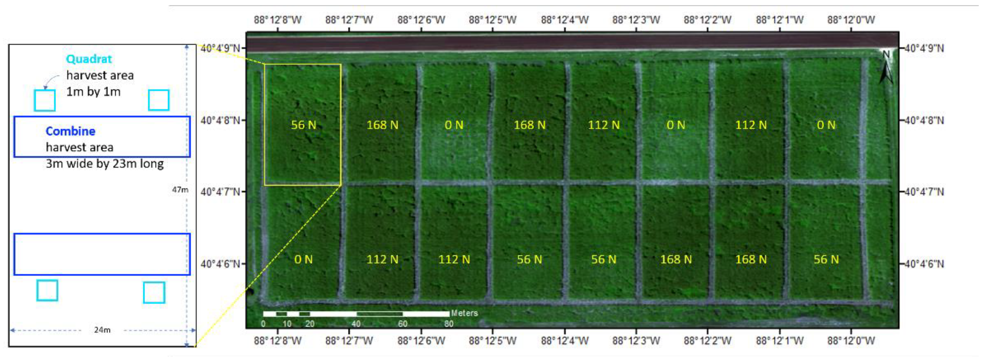
2.1. Study Site and Experimental Design

The field study was conducted on Flanagan silt loam (Fine, smectitic, mesic Aquic Argiudolls) at the University of Illinois Energy Farm (40.06869 N, −88.20133 W) in Urbana, IL, USA. The land capability class (LCC) of the site is 4 W-associated low soil fertility and poor drainage. These conditions limit conventional crop production; thus, the land is classified as marginal. A Miscanthus stand was established by planting rhizomes in 2009, which had an annual DM yield of <10 Mg ha−1 with no N application until the current study was initiated in 2018. The current trial was established on a portion of a 10 ha field with dimensions of 100 m (north/south direction) by 200 m (west/east direction) (Figure 1). The individual plots (47 m × 24 m) were arranged in a randomized complete block design with (RCBD) replicated four times. The treatments were four N application rates of 0, 56, 112, and 168 kg N ha−1 (hereafter referred to as 0 N, 56 N, 112 N, and 168 N, respectively) using urea as the N source. Fertilizer was applied in late April in both 2018 and 2019. Four quadrats (1 m × 1 m) were randomly placed in each plot (64 quadrats in total), immediately after fertilizer application.

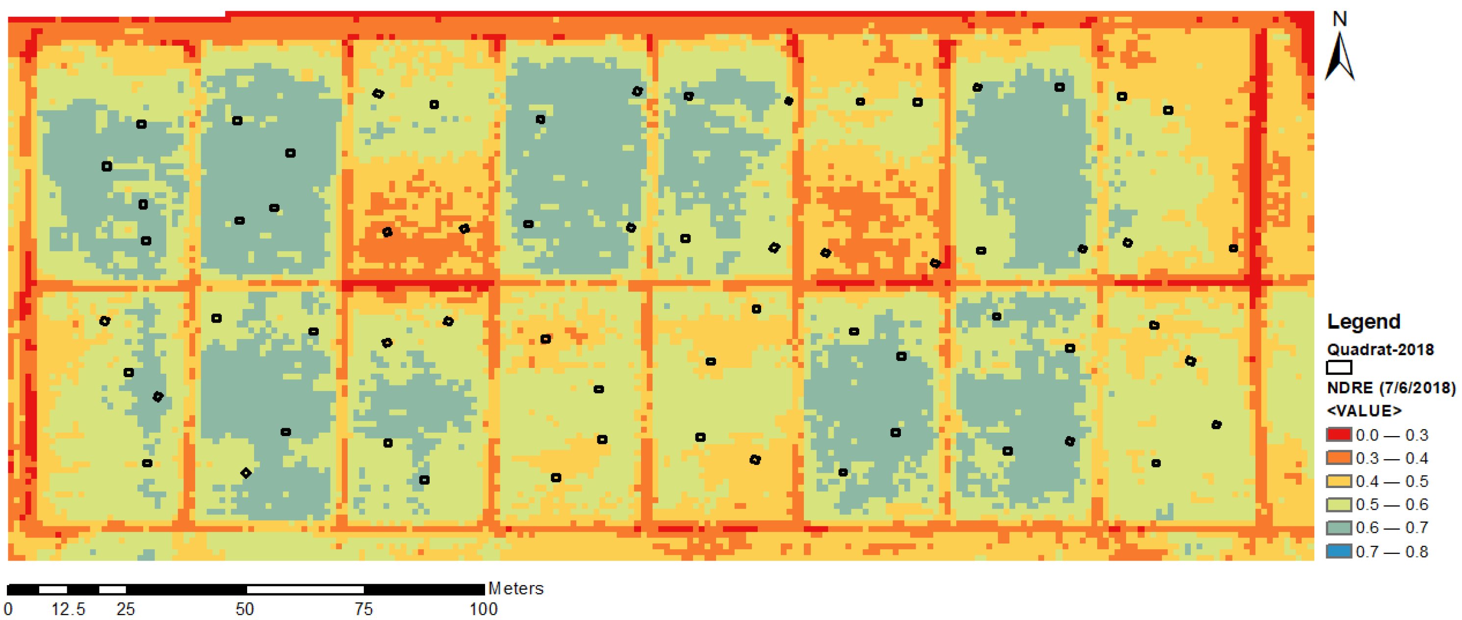
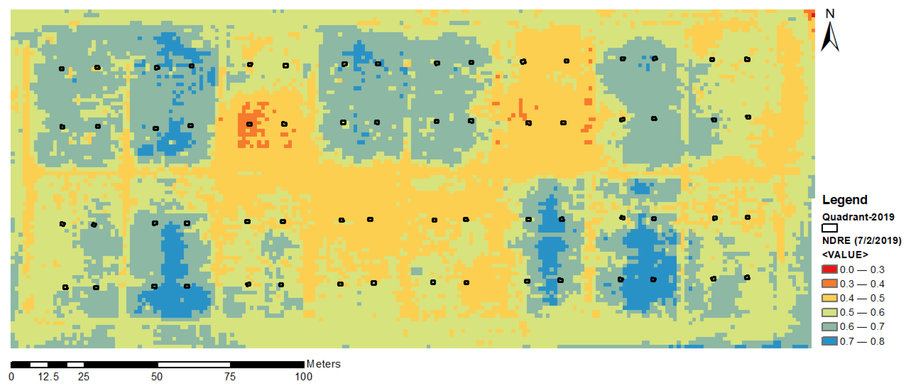
2.2. Drone Imagery Collection

Images were collected three times in 2018 and 2019 and are referred as the early (6 July in 2018 and July 2 in 2019), mid- (17 July in 2018 and 1 August in 2019), and late (31 August in 2018 and 18 September in 2019) summer growing seasons. Before and after drone flights, a reflectance panel was used for radiometric calibration. A Micasense Altum sensor was mounted on the drone to collect blue, green, red, red edge (RE), and near-infrared (NIR) bands with 5.2 cm/pixel per band. The wavelength specification was 475 nm center and 20 nm bandwidth for blue, 560 nm center and 20 nm bandwidth for green, 668 nm center and 10 nm bandwidth for red, 717 nm center and 10 nm bandwidth for RE, and 840 nm center and 40 nm bandwidth for NIR. The raw images of each flight were preprocessed in Pix4D Mapper and exported in a single GeoTIFF image. All images were aligned and georeferenced using the ground-control locations measured by a Trimble R12 GNSS (Trimble: Sunnyvale, CA, USA) in ArcGIS10.7.1 [34]. Vegetation indices (VIs) are the algebraic combination of several spectral bands (Table 1). The VI maps were calculated using the QGIS 3.10.2 raster calculator [35].

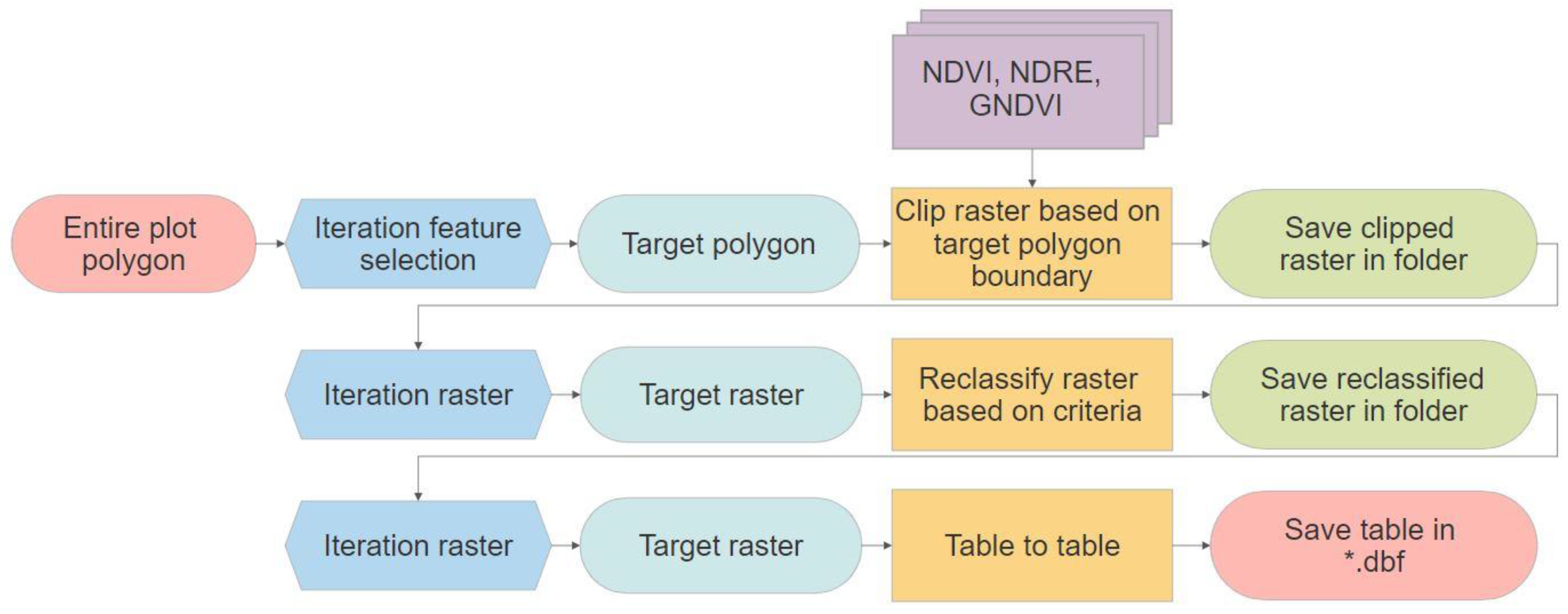
2.3. Reclassification of Vegetation Indices

The spatial distribution of crop stand health can be visually determined from VI maps. However, interpretation in the study was challenging due to the high resolution and variation within the harvested areas. Thus, to assess changes in Miscanthus coverage and, subsequently, stand health, the vegetation indices (ranging from −1 to 1) were reclassified into bare land (BL), unhealthy (UH), moderately healthy (MH) and very healthy (VH) using the model builder in ArcGIS (Table 2). The process involved three steps (Figure 2). First, the entire polygon map was broken down into individual polygons, and VIs were clipped from them. Here, a polygon is a quadrat or machinery harvest area (see Section 2.4). A total of 384 raster maps were generated form the quadrat-area polygons (64 quadrat areas × 3 UAV flights × 2 years), and 192 were obtained from the machinery harvest area (32 machinery harvest area × 3 UAV flights × 2 years). The second step involved the reclassification of the raster value into the four levels by utilizing the iteration raster function in the model builder to read the individual raster files. Finally, the reclassified VIs were expressed as cell counts for each level, and the percent of coverage for each plant level was calculated within each quadrat and machinery-harvest area.

2.4. Harvesting

Biomass yield estimation was done by harvesting overwintering biomass on February 28 and 24 in 2019 and 2020, respectively. Harvesting from all 64 quadrats was done by cutting the stems 10 cm from the ground and weighing them as fresh matter (FM) yield. A subsample (~1.0 kg) from each quadrat was weighed and oven-dried at 60 °C for 72 h to estimate dry matter (DM) yield.
Harvesting from the whole plot was done using a combine harvester (a tractor mounted with a Kemper forage chopper, Ames IA). Fresh biomass was obtained from two windrows (hereafter referred to as the machinery area) running in the east–west direction. Each machinery harvest area had a width of 3 m (equal to the length of the cutting table of the combine) and an average length of 23 m, effectively making 32 machinery harvest areas. The DM yield of the machinery harvest was determined from a subsample, following the same procedure as that used for estimating DM yield from the quadrats.

2.5. Statistical Analysis

Before conducting statistical tests, we explored any departures from normality of the variables: VIs (i.e., NDVI, NDRE, and GNDVI), FM, and DM yield. First, we fitted a mixed model using the generalized mixed model from the R package ‘lme4’ [42], with N treatment as fixed effect and block as random factors. Then, the Shapiro–Wilk normality test was performed on the model residuals. Quadrat data that departed from normal included all 2018 NDVI measurements, Aug and Sep 2019 NDVI, Sep 2019 GNDVI, and the 2019 DM yield. From the machinery-harvested areas, all NDVI data in 2018 also departed from normal, but only Sep NDVI was not normally distributed in 2019. To improve normality, Tukey’s ladder of powers was used to transform the data using the ‘TransformTukey’ function of the ‘rcompanion’ package [43].
To determine the effect of N treatments on VIs, FM yield, and DM yield, we conducted ANOVA using the generalized mixed model. Where N treatment was significant, the Tukey post hoc test was used to extract pairwise comparisons using the CLD function from the “emmeans” package [44]. All analyses of the quadrat and machine-harvested areas were conducted separately. To determine measurement differences between the quadrat and combine harvests, the non-parametric Mann–Whitney–Wilcoxon was performed between VIs and biomass yield from the two datasets. All statistical analyses were carried out in R version 4.0.0 [45]. Finally, the relationship between biomass and VIs was evaluated using simple linear regression. R2 values were used to determine the amount of variation explained by the linear model.

3. Results

3.1. Weather and Climate

The 2018 and 2019 monthly temperature and precipitation, as well as the 30-year averages (1987–2017) for Urbana, IL are shown in Table 3. The annual precipitation in 2018 (1169 mm) was higher than the long-term average of 1030 mm, whereas that in 2019 (1030 mm) was equal to the long-term average. Growing season (April–September) total precipitation was also higher in 2018 (667 mm) and lower in 2019 (577 mm) than the long-term average (611 mm). Average annual temperatures were 16.8 °C in 2018, 11.1 °C in 2019, and 11.5 °C for the long-term.

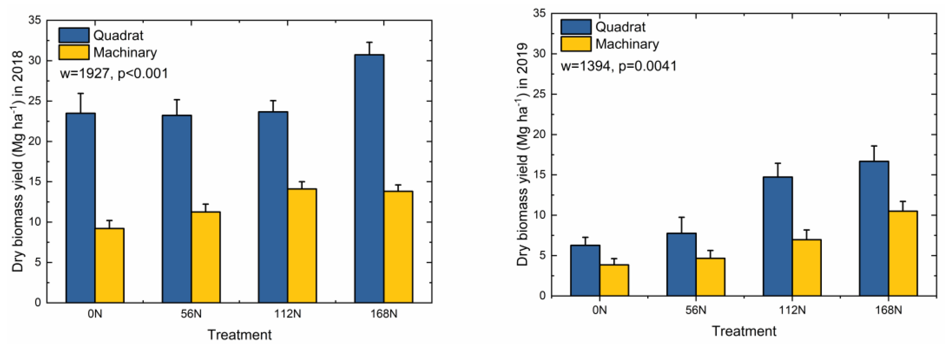
3.2. Effect of N Application on Biomass Yield and VIs

Average 2018 DM and FM yields were approximately twice those of 2019 (Figure 3). Significant differences in FM and DM yield due to N application were detected (Table 4 and Table 5). Biomass yields were greater in 168 N compared to 0 N. However, no differences were observed between 0 N and 56 N nor 112 N and 168 N. Both FM and DM yields harvested from the quadrats were higher than those from the machine-harvested areas in 2018 (both p < 0.001) and 2019 (p = 0.004 and p < 0.001, respectively) (Table 5).
All VIs showed significant differences due to N treatment in both 2018 and 2019 (Table 4 and Table 5). The average VIs increased as N application rates increased, although, as in the FM and DM yields, differences were not always significant between rates. Quadrat VIs showed no differences between 0 N and 56 N and between 112 N and 168 N application rates, but there were differences between 0 N and 168 N (Table 5). The VIs from machine-harvested areas also showed similar patterns (Table 4). Other than NDRE in early summer (p = 0.041) and late-summer GNDVI (p = 0.004) in 2019, no differences were observed between NDVI of quadrat and machine harvest areas (Table 6).

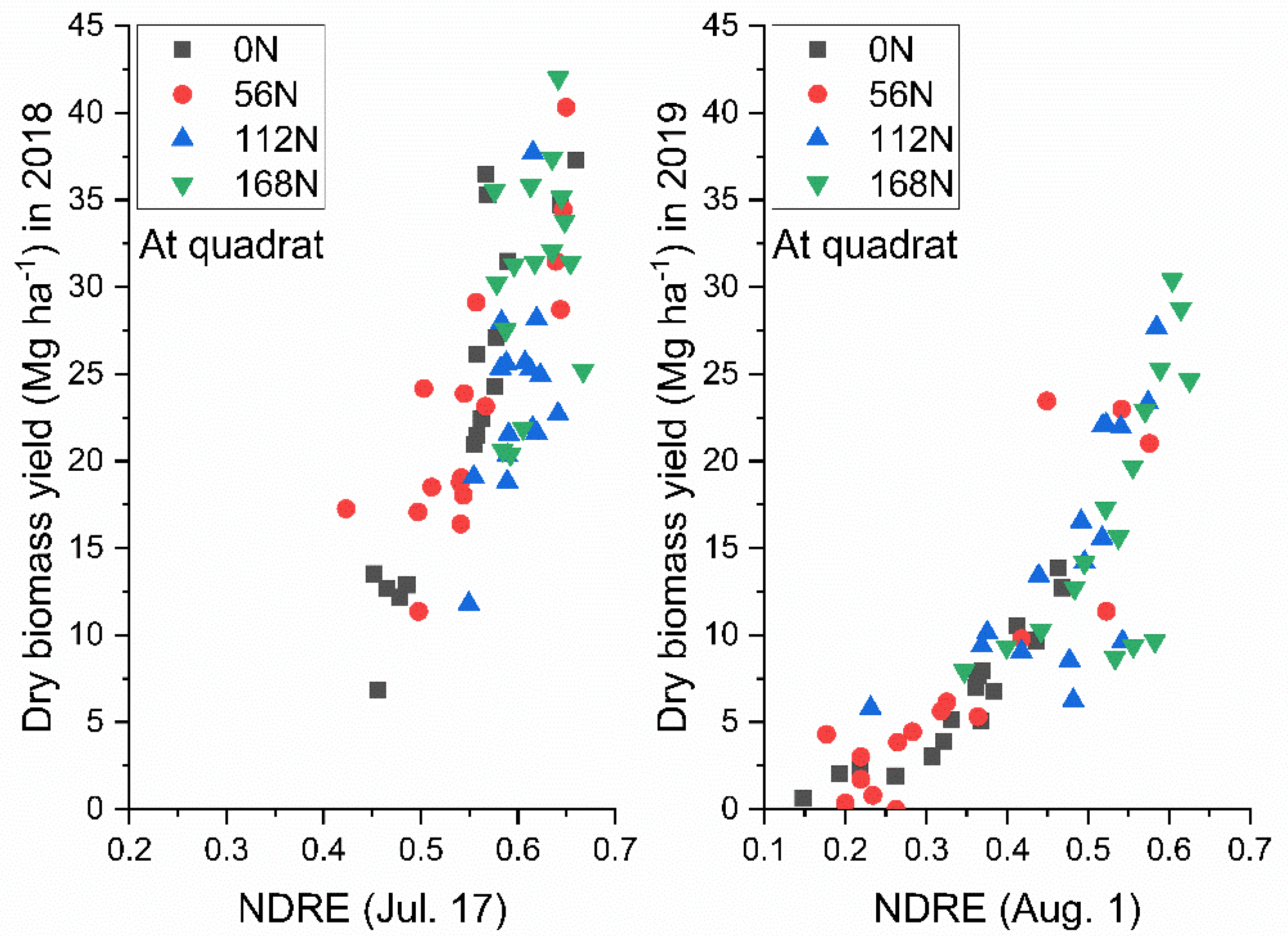
3.3. Linear Regression between Biomass Yield and Vegetation Indices

Overall, VIs were better correlated with biomass yield (both DM and FM) when measured from machine-harvested areas compared to quadrat-harvested areas (Table 7). Machine-harvested estimates of biomass yields showed the strongest correlations with the mid-growing-season measurements of NDRE (FM 0.87 in 2018 and 0.97 in 2019) and DM (0.89 in 2018 and 0.97 in 2019). GNDVI also showed good correlation with both FM and DM but was consistently lower than NDRE.

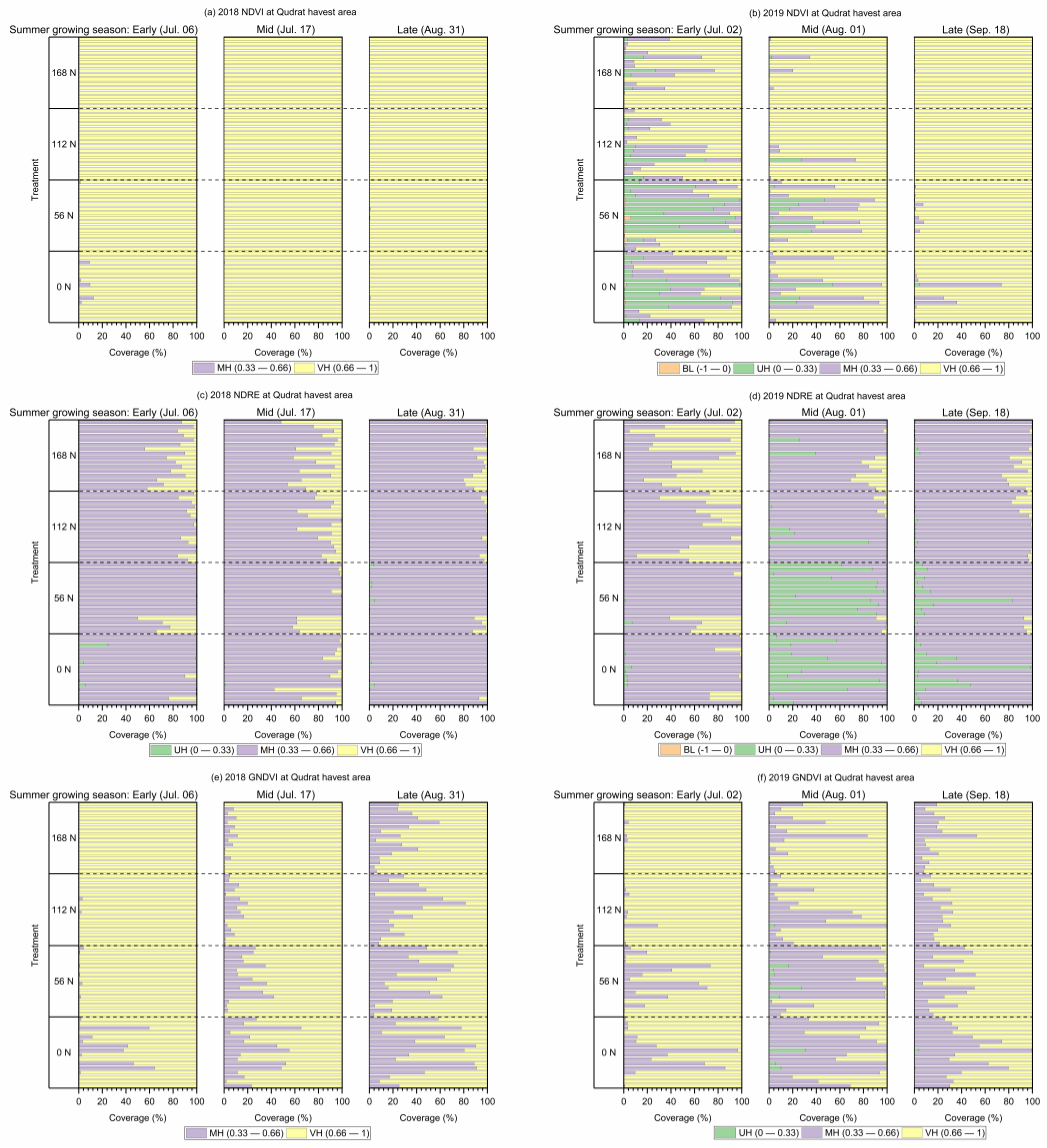
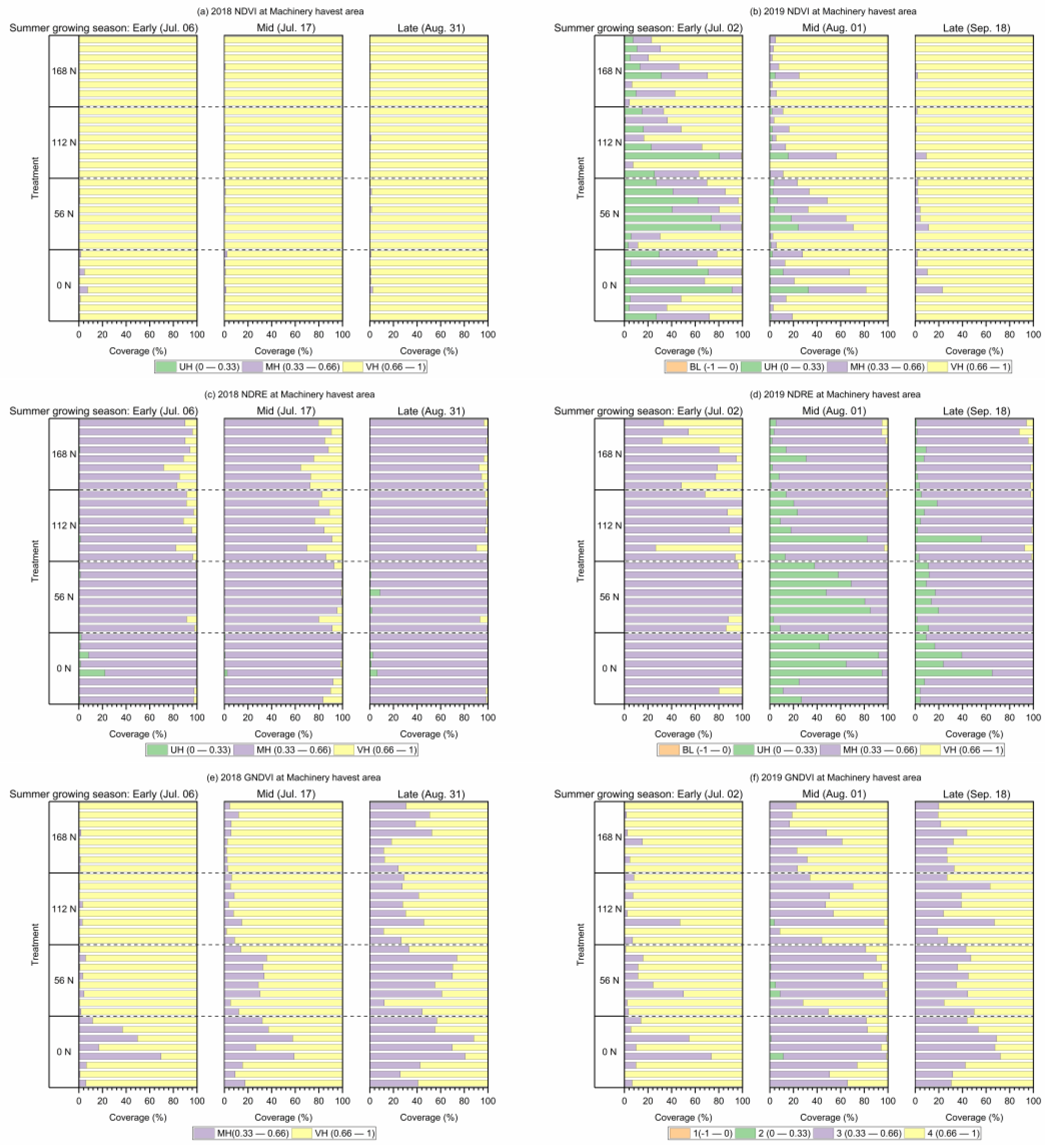
3.4. Plant Health Coverage Change under Different N Treatments

The reclassified NDVI from both quadrat- and machine-harvested areas in 2018 identified mostly VH stands throughout the growing season, with few discernible differences in health between the 56 N, 112 N, and 168 N treatments (Figure 4 and Figure 5). However, in 2019, NDVI measurements showed that UH to MH conditions dominated in the early-summer growing season, but stand health improved through the season (Figure 4 and Figure 5). In 2019, the 0 N treatment had a more noticeable proportion of UH and MH in early-summer-growing-season measurements (July). For instance, the coverage of stand rated lower than UH in July 2019 at approximately 30% in both quadrat- and machine-harvested areas (Figure 6). Conversely, only 4% and 10% of the 168 N treatment rated UH in the quadrat- and machine-harvested areas, respectively (Figure 6). However, late-summer-growing-season NDVI measurements (September) showed that 0 N and 56 N were dominated by VH (>91%) (Figure 4, Figure 5 and Figure 6).
Unlike NDVI, the NDRE results show the MH stand condition dominated (Figure 4 and Figure 5). In 2018, early July NDRE showed that about 25% of quadrat- and 22% of machine-harvested areas were UH in the 0 N treatment (Figure 6). Despite not being visible in the mid-summer growing season (mid-July), UH occurred again in 0 N (quadrat-harvested area, 5%; machine-harvested areas, 6%) and 56 N (quadrat-harvested areas, 3%; and machine-harvested area, 6%) treatments in the late-summer growing season (late August). In 2019, early July showed a high proportion of VH in the 112 N and 168 N treatments compared to the 0 N and 56 N treatments. Moreover, the mid-summer growing season (August) measurements showed a sharp increase in UH stand in the low-N treatments. For example, 42% of quadrat- and 51% of machine-harvested areas were UH in the 0 N treatment but reduced to 4% and 8%, respectively in the 168 N treatment. Late-growing-season (mid-September) NDRE had an increase in MH across all N treatments regardless of harvest area (Figure 6).
Neither BL nor UH was evident in the GNDVIs. Very healthy stand conditions dominated the early and mid-summer growing season GNDVI measurements in both years, although the 168 N treatment had a higher coverage compared to that of 0 N for both quadrat and machinery harvest areas (Figure 6). Subsequent GNDVI measurements in the mid- and late-summer growing seasons showed an increase in moderately healthy stand conditions and a reduction in very healthy conditions.

4. Discussion

Although some studies indicate that Miscanthus yield may not respond to N applications, consensus is building around moderate application rates as a strategy to boost Miscanthus yields [18,46]. Our study shows similar results, noting yield improvements between the 0 N at 168 N treatments but not between 0 N and 56 N. In 2018, there were no yield differences in machine-harvested DM yield between 112 N and 168 N, which is in agreement with the results reported by Parish et al. [47], who found no yield improvement beyond 112 kg N ha−1. Our results of no differences between 0 and 56 kg N ha−1 are similar to those reported by Lee et al. [46], who found Miscanthus yield did not change in certain locations under low rates of N (60 kg N ha−1). This indicates that site characteristics (e.g., soil and climate) play a key role in Miscanthus productivity in response to N application. The higher biomass yields in 2018 can be attributed to precipitation and temperature higher than long-term averages for the growing season [38].
Differences in VIs due to N treatment showed that all three VIs (NDVI, NDRE, and GNDVI) can distinguish nitrogen effects, irrespective of the size of the harvest area. However, N levels within a narrow range may not be differentiated using VIs; the VIs from 0 N and 56 N, as well as 112 N and 168 N, were consistently the same, whereas there were differences between 0 N and 168 N applications. Li et al. [28] also observed differences in VIs measured from sorghum with different N rates (0 and 95 kg N ha−1). A search of the literature did not identify other studies that focused on differences between VIs obtained from N treatment in perennial grasses. Thus, there is a need for additional studies that use VIs to discriminate between nitrogen application rates in perennial grass systems, including Miscanthus.
Nevertheless, the regression between VIs and biomass yields shows that mid-summer-growing-season (mid-July to August) measurements of NDRE provide a more consistent prediction of FM and DM yield of Miscanthus (ranged from 0.86 R2 to 0.97 R2). Studies have found that VIs reflecting peak greenness, collected from late June to early August, are most effective in forecasting crop yield [48,49,50]. Coefficient-of-determination values show that generally, mid-July to early August provides the best forecast of Miscanthus FM and DM. These results contrast with those reported by Li et al. [28] and Li et al. [51], who found that NDRE alone produced poorer forecasts of both switchgrass and sorghum yield relative to other indices, including NDVI. However, both studies used UAV images obtained late in the growing season (August to November), and the authors ultimately concluded that including other phenotypic traits in the regressions might improve their performance. Since Miscanthus usually achieves maximum growth in central Illinois in September [38], our findings suggest that NDRE is sensitive to differences in plant vigor due to N treatment during periods of peak Miscanthus growth (Figure 7). These findings also highlight the importance of mid-July to early August phenotypic measurements as indicators of potential DM yields of Miscanthus.
Whereas the VIs, DM, and FM from areas harvested by quadrat and machinery showed similar N-treatment response patterns, our results show that quadrat harvests overestimated both DM (52% in 2018 and 43% in 2019) and FM (47% in 2018 and 48% in 2019). Differences in yield can be attributed to the four quadrats not fully accounting for spatial heterogeneity of the Miscanthus stand (Figure 8). Tsutsumi et al. [52] showed that increasing the number and size of quadrat samples can increase the accuracy of biomass yield. Better coefficient-of-determination values between VIs and biomass from machine-harvested areas in our study suggest that the accuracy of biomass yield prediction may be improved from larger harvest areas. Indeed, our quadrat size of 1 m2 is a third of the sample size considered adequate for accurate and practical DM estimation [21]. The results of our study also indicate the need to establish reliable small-plot studies for estimating Miscanthus biomass yields. We recommend further research to clarify the adequate quadrat size for DM estimation.
Results from the VIs show an overall reduction in the stand health of Miscanthus in the low-N treatments (0 N and 56 N) between 2018 and 2019. In contrast, the 112 N and 168 N treatments had predominantly MH to VH stands in 2019. We assumed that there was N carryover from 2018 to 2019, as these plots received high N application for two years. We observed a significant winter injury and overall reduction in stand health, especially in the low-N treatments, which aligned with the VI results. The results contradict studies that found little impact of N on biomass yield and that where N effect is palpable, it eventually wanes over time [14,53]. Tejara et al. [15] found that N can impact Miscanthus productivity by increasing growing-season length and stand density. Lee et al. [46] and Zumpf et al. [54] also found N positively impacted the yield of Miscanthus over time. However, the data showing the positive impact of N on yield, including those of the current study, were obtained from relatively short-term studies. Additionally, we were not able to rule out an N carryover effect arising from the high N application rates over the two years. Thus, we recommend long-term studies to better determine N impact on Miscanthus biomass yield.
All three NDRE measurements in both growing seasons identified percentage changes in Miscanthus stand health over time by offering clearer contrasts of stand health ratings. In contrast, only early-July NDVI measurements clearly showed variances in stand heath status in 2019. This finding emphasizes the limitations of using NDVI to monitor stand health late in the season. In other studies, late-growing-season NDVI measurements reached saturation in dense plant canopies, as they become insensitive to high values of leaf area index [31,32,33].

5. Conclusions

Vegetation indices can be important tools for rapidly and cost-effectively predicting yield and stand health of perennial grasses. Our results show vegetation indices can distinguish between N treatments but may not be useful for N treatments within a narrow range of N rates. Our study also found that Miscanthus yield improved following application of N at 112 kg ha−1 and that NDRE is an ideal candidate for predicting both yield and stand health of Miscanthus. We conclude that N applied below the recommended rate will likely result in Miscanthus health deterioration over time. However, further studies are needed, to assess the long-term productivity of Miscanthus supplied with sufficient nitrogen. We recommend that future research focus on exploring the potential of image processing and deep learning using artificial intelligence (AI) technology to provide convincing performance in UAV remote sensing.

Author Contributions

Conceptualization, C.J. and D.L.; data curation, N.N., C.J., Z.R. and S.-H.L.; formal analysis, N.N. and C.J.; funding acquisition, D.L.; investigation, N.N., C.J., Z.R. and S.-H.L.; methodology, N.N. and C.J.; project administration, C.J. and D.L.; resources, D.L.; software, N.N. and C.J.; supervision, C.J. and D.L.; validation, N.N. and C.J.; visualization, C.J.; writing—original draft, N.N. and C.J.; writing—review and editing, N.N., C.J., C.-H.L., T.V. and D.L. All authors were informed about each step of manuscript processing, including submission, revision, revision reminder, etc., via emails from our system or assigned Assistant Editor. All authors have read and agreed to the published version of the manuscript.

Funding

This work was funded by the DOE Center for Advanced Bioenergy and Bioproducts Innovation (US Department of Energy, Office of Science, Office of Biological and Environmental Research under Award Number DE-SC0018420). Any opinions, findings, and conclusions or recommendations expressed in this publication are those of the author(s) and do not necessarily reflect the views of the U.S. Department of Energy.

Institutional Review Board Statement

Not applicable.

Informed Consent Statement

Not applicable.

Data Availability Statement

The data presented in this study are available on request from the authors.

Conflicts of Interest

The authors declare no conflict of interest.

References

  1. Hill, J.; Nelson, E.; Tilman, D.; Polasky, S.; Tiffany, D. Environmental, economic, and energetic costs and benefits of biodiesel and ethanol biofuels. Proc. Natl. Acad. Sci. USA 2006, 103, 11206–11210. [Google Scholar] [CrossRef] [PubMed] [Green Version]
  2. Pimentel, D.; Marklein, A.; Toth, M.A.; Karpoff, M.N.; Paul, G.S.; McCormack, R.; Kyriazis, J.; Krueger, T. Food Versus Biofuels: Environmental and Economic Costs. Hum. Ecol. 2009, 37, 1. [Google Scholar] [CrossRef]
  3. Ferrarini, A.; Serra, P.; Almagro, M.; Trevisan, M.; Amaducci, S. Multiple ecosystem services provision and biomass logistics management in bioenergy buffers: A state-of-the-art review. Renew. Sustain. Energy Rev. 2017, 73, 277–290. [Google Scholar] [CrossRef]
  4. Follett, R.F.; Kimble, J.; Pruessner, E.; Samson-Liebig, S.; Waltman, S. Soil organic carbon stocks with depth and land use at various US sites. SSSA Spec. Publ. 2009, 57, 29–46. [Google Scholar]
  5. Zumpf, C.; Ssegane, H.; Negri, M.C.; Campbell, P.; Cacho, J. Yield and Water Quality Impacts of Field-Scale Integration of Willow into a Continuous Corn Rotation System. J. Environ. Qual. 2017, 46, 811–818. [Google Scholar] [CrossRef] [PubMed] [Green Version]
  6. Cadoux, S.; Riche, A.B.; Yates, N.E.; Machet, J.-M. Nutrient requirements of Miscanthus × giganteus: Conclusions from a review of published studies. Biomass Bioenergy 2012, 38, 14–22. [Google Scholar] [CrossRef]
  7. Dohleman, F.G.; Long, S.P. More Productive Than Maize in the Midwest: How Does Miscanthus Do It? Plant. Physiol. 2009, 150, 2104–2115. [Google Scholar] [CrossRef] [Green Version]
  8. Dohleman, F.G.; Heaton, E.A.; Leakey, A.D.B.; Long, S.P. Does greater leaf-level photosynthesis explain the larger solar energy conversion efficiency of miscanthus relative to switchgrass? Plant Cell Environ. 2009, 32, 1525–1537. [Google Scholar] [CrossRef]
  9. Heaton, E.A.; Dohleman, F.G.; Long, S.P. Meeting US biofuel goals with less land: The potential of miscanthus. Glob. Chang. Biol. 2008, 14, 2000–2014. [Google Scholar] [CrossRef]
  10. Clifton-Brown, J.C.; Breuer, J.; Jones, M.B. Carbon mitigation by the energy crop, miscanthus. Glob. Chang. Biol. 2007, 13, 2296–2307. [Google Scholar] [CrossRef]
  11. Arnoult, S.; Brancourt-Hulmel, M. A Review on Miscanthus Biomass Production and Composition for Bioenergy Use: Genotypic and Environmental Variability and Implications for Breeding. BioEnergy Res. 2015, 8, 502–526. [Google Scholar] [CrossRef] [Green Version]
  12. Arundale, R.A.; Dohleman, F.G.; Heaton, E.A.; Mcgrath, J.M.; Voigt, T.B.; Long, S.P. Yields of Miscanthus × giganteus and Panicum virgatum decline with stand age in the Midwestern USA. Glob. Chang. Biol. Bioenergy 2014, 6, 1–13. [Google Scholar] [CrossRef]
  13. Arundale, R.A.; Dohleman, F.G.; Voigt, T.B.; Long, S.P. Nitrogen Fertilization Does Significantly Increase Yields of Stands of Miscanthus × giganteus and Panicum virgatum in Multiyear Trials in Illinois. Bioenergy Res. 2014, 7, 408–416. [Google Scholar] [CrossRef]
  14. Chen, H.; Dai, Z.; Jager, H.I.; Wullschleger, S.D.; Xu, J.; Schadt, C.W. Influences of nitrogen fertilization and climate regime on the above-ground biomass yields of miscanthus and switchgrass: A meta-analysis. Renew. Sustain. Energy Rev. 2019, 108, 303–311. [Google Scholar] [CrossRef]
  15. Tejera, M.D.; Miguez, F.E.; Heaton, E.A. The older plant gets the sun: Age-related changes in Miscanthus × giganteus phenology. GCB Bioenergy 2021, 13, 4–20. [Google Scholar] [CrossRef]
  16. Maughan, M.; Bollero, G.; Lee, D.K.; Darmody, R.; Bonos, S.; Cortese, L.; Murphy, J.; Gaussoin, R.; Sousek, M.; Williams, D.; et al. Miscanthus giganteus productivity: The effects of management in different environments. Glob. Chang. Biol. Bioenergy 2012, 4, 253–265. [Google Scholar] [CrossRef]
  17. Christian, D.G.; Riche, A.B.; Yates, N.E. Growth, yield and mineral content of Miscanthus × giganteus grown as a biofuel for 14 successive harvests. Ind. Crops Prod. 2008, 28, 320–327. [Google Scholar] [CrossRef]
  18. Lee, M.S.; Wycislo, A.; Guo, J.; Lee, D.K.; Voigt, T. Nitrogen Fertilization Effects on Biomass Production and Yield Components of Miscanthus × giganteus. Front. Plant Sci. 2017, 8, 544. [Google Scholar] [CrossRef] [Green Version]
  19. Yost, M.A.; Randall, B.K.; Kitchen, N.R.; Heaton, E.A.; Myers, R.L. Yield Potential and Nitrogen Requirements of Miscanthus × giganteus on Eroded Soil. Agron. J. 2017, 109, 684–695. [Google Scholar] [CrossRef] [Green Version]
  20. Cichorz, S.; Gośka, M.; Litwiniec, A. Miscanthus: Genetic Diversity and Genotype Identification Using ISSR and RAPD Markers. Mol. Biotechnol. 2014, 56, 911–924. [Google Scholar] [CrossRef] [Green Version]
  21. Knörzer, H.; Hartung, K.; Piepho, H.P.; Lewandowski, I. Assessment of variability in biomass yield and quality: What is an adequate size of sampling area for miscanthus? GCB Bioenergy 2013, 5, 572–579. [Google Scholar] [CrossRef]
  22. Tang, Y.; Dananjayan, S.; Hou, C.; Guo, Q.; Luo, S.; He, Y. A survey on the 5G network and its impact on agriculture: Challenges and opportunities. Comput. Electron. Agric. 2021, 180, 105895. [Google Scholar] [CrossRef]
  23. Henik, J.J. Utilizing NDVI and Remote Sensing Data to Identify Spatial Variability in Plant Stress as Influenced by Management. Master’s Thesis, Iowa State University, Ames, IA, USA, 2012. [Google Scholar] [CrossRef]
  24. Teal, R.K.; Tubana, B.; Girma, K.; Freeman, K.W.; Arnall, D.B.; Walsh, O.; Raun, W.R. In-Season Prediction of Corn Grain Yield Potential Using Normalized Difference Vegetation Index. Agron. J. 2006, 98, 1488–1494. [Google Scholar] [CrossRef] [Green Version]
  25. Shafian, S.; Rajan, N.; Schnell, R.; Bagavathiannan, M.; Valasek, J.; Shi, Y.; Olsenholler, J. Unmanned aerial systems-based remote sensing for monitoring sorghum growth and development. PLoS ONE 2018, 13, e0196605. [Google Scholar] [CrossRef] [Green Version]
  26. Seo, B.; Lee, J.; Lee, K.D.; Hong, S.; Kang, S. Improving remotely-sensed crop monitoring by NDVI-based crop phenology estimators for corn and soybeans in Iowa and Illinois, USA. Field Crop Res. 2019, 238, 113–128. [Google Scholar] [CrossRef]
  27. Kayad, A.; Sozzi, M.; Gatto, S.; Marinello, F.; Pirotti, F. Monitoring Within-Field Variability of Corn Yield using Sentinel-2 and Machine Learning Techniques. Remote Sens. 2019, 11, 2873. [Google Scholar] [CrossRef] [Green Version]
  28. Li, J.; Shi, Y.; Veeranampalayam-Sivakumar, A.N.; Schachtman, D.P. Elucidating Sorghum Biomass, Nitrogen and Chlorophyll Contents with Spectral and Morphological Traits Derived from Unmanned Aircraft System. Front. Plant Sci. 2018, 9, 1406. [Google Scholar] [CrossRef]
  29. Foster, A.; Kakani, V.; Ge, J.; Mosali, J. Predicting biomass yield in bioenergy crop production systems using canopy NDVI. In Proceedings of the Sun Grant National Conference: Science for Biomass Feedstock Production and Utilization, New Orleans, LA, USA, 2–5 October 2012. [Google Scholar]
  30. Amaral, L.R.; Molin, J.P.; Portz, G.; Finazzi, F.B.; Cortinove, L. Comparison of crop canopy reflectance sensors used to identify sugarcane biomass and nitrogen status. Precis. Agric. 2015, 16, 15–28. [Google Scholar] [CrossRef]
  31. Chen, P.-Y.; Fedosejevs, G.; Tiscareño-López, M.; Arnold, J.G. Assessment of MODIS-EVI, MODIS-NDVI and VEGETATION-NDVI Composite Data Using Agricultural Measurements: An Example at Corn Fields in Western Mexico. Environ. Monit. Assess. 2006, 119, 69–82. [Google Scholar] [CrossRef]
  32. Gu, Y.; Wylie, B.K.; Howard, D.M.; Phuyal, K.P.; Ji, L. NDVI saturation adjustment: A new approach for improving cropland performance estimates in the Greater Platte River Basin, USA. Ecol. Indic. 2013, 30, 1–6. [Google Scholar] [CrossRef]
  33. Van Der Meer, F.; Bakker, W.; Scholte, K.; Skidmore, A.; De Jong, S.; Clevers, J.; Addink, E.; Epema, G. Spatial scale variations in vegetation indices and above-ground biomass estimates: Implications for MERIS. Int. J. Remote Sens. 2001, 22, 3381–3396. [Google Scholar] [CrossRef]
  34. Cao, Q.; Miao, Y.; Shen, J.; Yu, W.; Yuan, F.; Cheng, S.; Huang, S.; Wang, H.; Yang, W.; Liu, F. Improving in-season estimation of rice yield potential and responsiveness to topdressing nitrogen application with Crop Circle active crop canopy sensor. Precis. Agric. 2016, 17, 136–154. [Google Scholar] [CrossRef]
  35. Wang, F.M.; Huang, J.F.; Tang, Y.L.; Wang, X.Z. New vegetation index and its application in estimating leaf area index of rice. Rice Sci. 2007, 14, 195–203. [Google Scholar] [CrossRef]
  36. Beale, C.V.; Long, S.P. Seasonal dynamics of nutrient accumulation and partitioning in the perennial C4-grasses Miscanthus × giganteus and Spartina cynosuroides. Biomass Bioenergy 1997, 12, 419–428. [Google Scholar] [CrossRef]
  37. Heaton, E.A.; Flavell, R.B.; Mascia, P.N.; Thomas, S.R.; Dohleman, F.G.; Long, S.P. Herbaceous energy crop development: Recent progress and future prospects. Curr. Opin. Biotechnol. 2008, 19, 202–209. [Google Scholar] [CrossRef]
  38. Heaton, E.A.; Dohleman, F.G.; Míguez, A.; Juvik, J.A.; Lozovaya, V.V.; Widholm, J.M.; Zabotina, O.A.; McIsaac, G.F.; David, M.B.; Voigt, T.B. Miscanthus: A Promising Biomass Crop. Adv. Bot. Res. 2010, 56, 75–137. [Google Scholar]
  39. Rouse, J.W. Monitoring Vegetation Systems in the Great Plains with ERTS; NASA: Washington, DC, USA, 1974. Available online: https://ntrs.nasa.gov/search.jsp?R=19740022614 (accessed on 7 February 2021).
  40. Hansen, P.; Schjoerring, J. Reflectance measurement of canopy biomass and nitrogen status in wheat crops using normalized difference vegetation indices and partial least squares regression. Remote Sens. Environ. 2003, 86, 542–553. [Google Scholar] [CrossRef]
  41. Gitelson, A.A.; Kaufman, Y.J.; Merzlyak, M.N. Use of a green channel in remote sensing of global vegetation from EOS-MODIS. Remote Sens. Environ. 1996, 58, 289–298. [Google Scholar]
  42. Bates, D.; Maechler, M.; Bolker, B.; Walker, S. Fitting linear mixed-effects models using lme4. J. Stat. Softw. 2015, 65, 1–48. [Google Scholar] [CrossRef]
  43. Mangiafico, S. rcompanion: Functions to Support Extension Education Program Evaluation, R Package Version 2.4.1. CRAN. 2022. Available online: https://CRAN.R-project.org/package=rcompanion (accessed on 9 December 2021).
  44. Lenth, R.V. emmeans: Estimated Marginal Means, aka Least-Squares Means, R Package Version 1.5.4. CRAN. 2022. Available online: https://CRAN.R-project.org/package=emmeans (accessed on 9 December 2021).
  45. R Core Team. R: A Language and Environment for Statistical Computing; R Foundation for Statistical Computing: Vienna, Austria, 2020; Available online: https://www.R-project.org/ (accessed on 9 December 2021).
  46. Lee, D.K.; Aberle, E.; Anderson, E.K.; Anderson, W.; Baldwin, B.S.; Baltensperger, D.; Barrett, M.; Blumenthal, J.; Bonos, S.; Bouton, J. Biomass production of herbaceous energy crops in the United States: Field trial results and yield potential maps from the multiyear regional feedstock partnership. GCB Bioenergy 2018, 10, 698–716. [Google Scholar] [CrossRef]
  47. Parrish, A.S.; Lee, M.-S.; Voigt, T.B.; Lee, D.K. Miscanthus × giganteus Responses to Nitrogen Fertilization and Harvest Timing in Illinois, USA. BioEnergy Res. 2021, 14, 1126–1135. [Google Scholar] [CrossRef]
  48. Bolton, D.K.; Friedl, M.A. Forecasting crop yield using remotely sensed vegetation indices and crop phenology metrics. Agric. For. Meteorol. 2013, 173, 74–84. [Google Scholar] [CrossRef]
  49. Mkhabela, M.; Bullock, P.; Raj, S.; Wang, S.; Yang, Y. Crop yield forecasting on the Canadian Prairies using MODIS NDVI data. Agric. For. Meteorol. 2011, 151, 385–393. [Google Scholar] [CrossRef]
  50. Basnyat, P.; McConkey, B.; Lafond, G.R.; Moulin, A.; Pelcat, Y. Optimal time for remote sensing to relate to crop grain yield on the Canadian prairies. Can. J. Plant Sci. 2004, 84, 97–103. [Google Scholar]
  51. Li, F.; Piasecki, C.; Millwood, R.J.; Wolfe, B.; Mazarei, M.; Stewart, C.N. High-Throughput Switchgrass Phenotyping and Biomass Modeling by UAV. Front. Plant Sci. 2020, 11, 574073. [Google Scholar] [CrossRef]
  52. Tsutsumi, M.; Itano, S.; Shiyomi, M. Number of samples required for estimating herbaceous biomass. Rangel. Ecol. Manag. 2007, 60, 447–452. [Google Scholar] [CrossRef]
  53. Davis, M.P.; David, M.B.; Voigt, T.B.; Mitchell, C.A. Effect of nitrogen addition on Miscanthus × giganteus yield, nitrogen losses, and soil organic matter across five sites. GCB Bioenergy 2015, 7, 1222–1231. [Google Scholar] [CrossRef] [Green Version]
  54. Zumpf, C.; Lee, M.S.; Thapa, S.; Guo, J.; Mitchell, R.; Volenec, J.J.; Lee, D. Impact of warm-season grass management on feedstock production on marginal farmland in Central Illinois. GCB Bioenergy 2019, 11, 1202–1214. [Google Scholar] [CrossRef] [Green Version]
Figure 1. Geographic location of the study area and experimental design for subplots. The RGB imagery is from 6 July 2018, and the spacing between subplots is 3 m. Coordinates are referred to GCS_WGS_1984.
Remotesensing 14 01435 g001
Figure 2. The process of categorizing Miscanthus stands in four categories (bare land or dead plants (BL), less healthy plants (UH), moderately healthy plants (MH), and very healthy plants (VH)) using Model builder in ArcGIS10.7.1. The target polygon means the boundary of shapefile about each quadrat and machinery-harvest area. The target raster indicates individual NDVI, NDRE, and GNDVI map. The *.dbf represents the dBase database file.
Remotesensing 14 01435 g002
Figure 3. Dry biomass yield of Miscanthus in 2018 and 2019 growing seasons estimated from the hand-harvested 1 m × 1 m quadrats and the machine-harvested 3 m × 23 m area.
Remotesensing 14 01435 g003
Figure 4. Plant stand health condition coverage corresponding to the reclassified vegetation indices in quadrat-harvested areas in 2018 and 2019.
Remotesensing 14 01435 g004
Figure 5. Plant stand health condition coverage corresponding to the reclassified vegetation indices in machine-harvested areas in 2018 and 2019.
Remotesensing 14 01435 g005
Figure 6. Vegetative indices in early growing season show differences in stand health between the lowest (0 N kg ha−1) and highest (168 N kg ha−1) N treatments in 2018 and 2019. The darker color indicates very healthy (VH) stands.
Remotesensing 14 01435 g006
Figure 7. Nitrogen response was observed in the relationship between NDRE and dry biomass during the mid-summer growing season in 2018 and 2019. Biomass yield and plant stand health improved with increasing N fertilization.
Remotesensing 14 01435 g007
Figure 8. Aggregated NDRE maps during the early-summer growing season (6 July 2018 and 2 July 2019) with 1 m × 1 m resolution and quadrat locations in 2018 and 2019.
Remotesensing 14 01435 g008aRemotesensing 14 01435 g008b
Table 1. Standard formulas used to calculate vegetation indices (VIs) obtained from survey of Miscanthus using unmanned aerial vehicles (UAVs) in the 2018 and 2019 growing season in Urbana, IL, USA.
IndexNDVINDREGNDVI
Equation(NIR − RED)/(NIR + RED)(NIR − RE)/(NIR + RE)(NIR − GREEN)/(NIR + GREEN)
DescriptionNormalized Difference Vegetation IndexNormalized Difference Red EdgeGreen NDVI
Reference[39][40][41]
Table 2. Stand health classification of Miscanthus from reclassified vegetation indices (VIs: NDVI, NDRE, and GNDVI) obtained during UAV flights in the 2018 and 2019 growing season in Urbana, IL, USA.
Vegetation Index Range−1–00–0.330.33–0.660.66–1
DescriptionBare land/Dead plants (BL)Unhealthy plant
(UH)
Moderately healthy plant
(MH)
Very healthy plant
(VH)
Table 3. Monthly precipitation and maximum, minimum, and average temperatures in 2018 and 2019 in Urbana, IL, USA. The weather data were obtained from National Oceanic and Atmospheric Administration (NOAA) at Willard Airport Station.
Month2018201930-Year Average
Precipitation (mm)Temperature (°C)Precipitation (mm)Temperature (°C)Precipitation (mm)Temperature (°C)
January28.0−5.298.0−4.557.0−2.8
February155.0−0.149.0−1.258.2−0.6
March81.03.3129.02.771.75.2
April59.07.2124.011.394.511.5
May88.021.7155.017.3122.517.4
June210.023.771.021.9115.522.5
July85.023.586.025.2109.224
August105.024.156.02389.023.1
September120.021.785.022.380.719.3
October58.012.5127.012.183.312.7
November94.01.949.02.282.35.7
December86.01.246.01.366.3−0.5
Table 4. Average NDVI, NDRE, GNDVI, dry matter (DM) yield, and fresh matter (FM) (Mg ha−1) yield in response to nitrogen in 2018 and 2019 obtained from four 1 m × 1 m quadrats in Urbana, IL, USA. Numbers in parenthesis indicate standard error of the differences in means when analyzed by sampling date. Different letters indicate statistical differences in means due to N at p < 0.05.
2018
N RateNDVINDREGNDVIYield
EarlyMidLateEarlyMidLateEarlyMidLateFM
(Mg ha−1)
DM
(Mg ha−1)
July 6July 17August 31July 6July 17August 31July 6July 17August 31
0 N0.86 (0.010) a0.89 (0.006) a0.85 (0.010) a0.50 (0.020) a0.55 (0.0158) a0.48 (0.015) a0.72 (0.013) a0.70 (0.009) a0.66 (0.011) a26.10 (2.66) a23.49 (2.460) a
56 N0.88 (0.01) ab0.90 (0.003) ab0.86 (0.0071) a0.54 (0.018) ab0.553 (0.02)a0.49 (0.018) a0.76 (0.007) b0.72 (0.008) ab0.68 (0.009) ab25.7 (2.09) a23.23 (1.936) a
112 N0.89 (0.003) bc0.90 (0.002) b0.88 (0.005) b0.58 (0.01) bc0.60 (0.0062) b0.54 (0.010) b0.77 (0.004) bc0.74 (0.005) bc0.69 (0.008) b25.6 (1.35) a23.66 (1.385) a
168 N0.90 (0.002) c0.905 (0.002) b0.89 (0.003) b0.62 (0.007) c0.62 (0.007) b0.57 (0.008) b0.79 (0.003) c0.75 (0.004) c0.70 (0.007) b33.20 (1.64) b30.73 (1.556) b
Mean0.880.900.870.560.580.520.760.730.6827.6825.28
ANOVA
N ratep < 0.001p < 0.001p < 0.001p < 0.001p < 0.001p < 0.001p < 0.001p < 0.001p < 0.001p = 0.002p = 0.001
2019
N RateNDVINDREGNDVIYield
EarlyMidLateEarlyMidLateEarlyMidLateFM
(Mg ha−1)
DM
(Mg ha−1)
July 2August 1September 18July 2August 1September 18July 2August 1September 18
0 N0.51 (0.051) a0.72 (0.042) a0.83 (0.023) a0.51 (0.020) a0.34 (0.023) a0.40 (0.016) a0.72 (0.017) a0.59 (0.024) a0.66 (0.013) a7.91 (1.28) a6.27 (0.993) a
56 N0.44 (0.06) a0.68 (0.046) a0.86 (0.010) a0.54 (0.020) a0.34 (0.032) a0.44 (0.016) a0.73 (0.018) a0.58 (0.028) a0.70 (0.009) a9.49 (2.47) a7.76 (1.984) b
112 N0.69 (0.038) b0.86 (0.026) b0.90 (0.003) b0.62 (0.013) b0.47 (0.023) b0.50 (0.010) b0.80 (0.010) b0.69 (0.018) b0.72 (0.006) b18.20 (2.05) b14.73 (1.713) bc
168 N0.76 (0.032) b0.88 (0.016) b0.90 (0.005) b0.66 (0.012) b0.53 (0.020) b0.53 (0.013) b0.83 (0.009) b0.73 (0.013) b0.74 (0.008) b20.20 (2.27) b16.67 (1.916) c
Mean0.600.790.870.580.420.470.770.650.7013.9611.36
ANOVA
N ratep < 0.001p < 0.001p < 0.001p < 0.001p < 0.001p < 0.001p < 0.001p < 0.001p < 0.001p < 0.001p < 0.001
Table 5. Average NDVI, NDRE, GNDVI, and dry matter (DM) yield, and fresh matter (FM) yield (Mg ha−1) in response to nitrogen in 2018 and 2019 obtained from two 3 m x 23 m machine harvest areas in Urbana, IL, USA. Numbers in parenthesis indicate standard error of the differences in means when analyzed by date. Different letters indicate statistical differences in means due to N at p < 0.05.
2018
N RateNDVINDREGNDVIYield
EarlyMidLateEarlyMidLateEarlyMidLateFM
(Mg ha−1)
DM
(Mg ha−1)
July 6July 17August 31July 6July 17August 31July 6July 17August 31
0 N0.84 (0.012) a0.88 (0.008) a0.84 (0.014) a0.47 (0.023) a0.52 (0.018) a0.41 (0.018) a0.70 (0.015) a0.69 (0.012) a0.65 (0.011) a11.7 (1.09) a9.21 (0.987) a
56 N0.88 (0.004) b0.89 (0.004) ab0.85 (0.011) a0.52 (0.016) a0.54 (0.015) a0.48 (0.020) a0.74 (0.007) b0.70 (0.008) a0.657 (0.012) a13.9 (1.1) ab11.26 (0.961) ab
112 N0.89 (0.001) bc0.90 (0.002) bc0.88 (0.003) b0.58 (0.009) b0.60 (0.007) b0.54 (0.011) b0.77 (0.005) bc0.74 (0.004) b0.69 (0.006) b16.4 (1.01) b14.12 (0.876) b
168 N0.90 (0.001) c0.90 (0.002) c0.88 (0.004) b0.602 (0.006) b0.61 (0.0073) b0.55 (0.012) b0.78 (0.003) c0.75 (0.004) b0.69 (0.009) b16.8 (1.00) b13.81 (0.806) b
Mean0.880.890.870.540.570.510.750.720.6714.7212.1
ANOVA
N ratep < 0.001p < 0.001p < 0.001p < 0.001p < 0.001p < 0.001p < 0.001p < 0.001p < 0.001p = 0.002p < 0.001
2019
N RateNDVINDREGNDVIYield
EarlyMidLateEarlyMidLateEarlyMidLateFM
(Mg ha−1)
DM
(Mg ha−1)
July 2August 1September 18July 2August 1September 18July 2August 1September 18
0 N0.49 (0.064) a0.70 (0.045) a0.83 (0.019) a0.50 (0.020) a0.32 (0.024) a0.39 (0.018) a0.71 (0.017) a0.58 (0.024) a0.66 (0.010) a4.23 (0.852) a3.86 (0.770) a
56 N0.45 (0.071) a0.69 (0.044) a0.85 (0.009) a0.53 (0.020) ab0.33 (0.026) a0.42 (0.007) a0.73 (0.015) ab0.58 (0.025) a0.68 (0.005) a5.16 (1.09) a4.66 (0.965) a
112 N0.60 (0.063) ab0.80 (0.033) ab0.87 (0.014) ab0.57 (0.024) bc0.41 (0.028) b0.44 (0.023) ab0.76 (0.017) bc0.65 (0.023) b0.69 (0.012) ab7.81 (1.42) ab6.96 (1.223) a
168 N0.70 (0.039) b0.85 (0.018) b0.89 (0.006) b0.63 (0.018) c0.47 (0.017) b0.48 (0.012) b0.80 (0.012) c0.69 (0.012) b0.707 (0.007) b11.66 (1.36) b10.50 (1.210) b
Mean0.560.760.860.560.380.430.750.620.687.216.50
ANOVA
N ratep = 0.002p < 0.001p < 0.001p < 0.001p < 0.001p < 0.001p < 0.001p < 0.001p < 0.001p < 0.001p < 0.001
Table 6. Mann–Whitney–Wilcoxon results showing significant differences of VIs collected over three flights between four nitrogen treatments during the early-, mid-, and late-summer growing season in 2018 and 2019.
YearSummer Growing Season (Date)VIsWp-Value
2018Early (6 Jul)NDVI11940.188
NDRE12540.075
GNDVI12270.116
Mid (17 Jul)NDVI12180.133
NDRE11430.357
GNDVI11700.258
Late (31 Aug)NDVI12120.145
NDRE11160.477
GNDVI12400.094
2019Early (2 Jul)NDVI11840.215
NDRE12880.041
GNDVI12250.119
Mid (1 Aug)NDVI12250.119
NDRE12420.091
GNDVI13450.013
Late (18 Sep)NDVI12340.104
NDRE12660.061
GNDVI13950.004
Table 7. R2 between fresh (FM, Mg ha−1) and dry matter (DM, Mg ha−1) of Miscanthus, as well as corresponding vegetation Indices (NDVI, NDRE, GNDVI) from quadrat areas (n = 64) and machine-harvested areas (n = 32) obtained from unmanned aerial vehicle images collected over three flights in 2018 and 2019.
Summer Growing Season
(Flight Date)
VIs20182019
FMDMFMDM
QuadratMachineryQuadratMachineryQuadratMachineryQuadratMachinery
Early
(6 July/
2 July)
NDVI0.790.790.790.820.920.930.920.93
NDRE0.820.870.820.900.900.960.890.96
GNDVI0.820.870.820.900.910.960.900.96
Mid
(17 July/
1 August)
NDVI0.780.810.780.850.860.930.850.93
NDRE0.860.870.860.890.920.970.920.97
GNDVI0.840.870.850.890.900.950.900.95
Late
(31 August/
18 September)
NDVI0.840.840.840.860.780.910.780.91
NDRE0.850.890.840.920.880.900.880.90
GNDVI0.840.870.840.890.810.850.810.85
All results showed significant differences (p < 0.001).
Publisher’s Note: MDPI stays neutral with regard to jurisdictional claims in published maps and institutional affiliations.

