Article

A Visual Compass Based on Point and Line Features for UAV High-Altitude Orientation Estimation

State Key Laboratory of Industrial Control Technology, College of Control Science and Engineering, Zhejiang University, Hangzhou 310027, China
*
Author to whom correspondence should be addressed.
Remote Sens. 2022, 14(6), 1430; https://doi.org/10.3390/rs14061430
Submission received: 20 January 2022 / Revised: 23 February 2022 / Accepted: 4 March 2022 / Published: 16 March 2022

Abstract

:
The accurate and reliable high-altitude orientation estimation is of great significance for unmanned aerial vehicles (UAVs) localization, and further assists them to conduct some fundamental functions, such as aerial mapping, environmental monitoring, and risk management. However, the traditional orientation estimation is susceptible to electromagnetic interference, high maneuverability, and substantial scale variations. Hence, this paper aims to present a new visual compass algorithm to estimate the orientation of a UAV employing the appearance and geometry structure of the point and line features in the remote sensing images. In this study, a coarse-to-fine feature tracking method is used to locate the matched keypoints precisely. An LK-ZNCC algorithm is proposed to match line segments in real-time. A hierarchical fusion method for point and line features is designed to expand the scope of the usage of this system. Many comparative experiments between this algorithm and others are conducted on a UAV. Experimental results show that the proposed visual compass algorithm is a reliable, precise, and versatile system applicable to other UAV navigation systems, especially when they do not work in particular situations.

Graphical Abstract

1. Introduction

Unmanned Aerial Vehicles (UAVs) have gained great popularity recently in many remote sensing tasks, like 3D terrain analysis, slope stability, mass movement hazard, and risk management [1]. A reliable and accurate orientation estimation approach plays a critical role in both controlling UAVs and guaranteeing the performance of various remote sensing tasks. However, the orientation estimation at high altitude faces challenges due to the extreme working condition, where electromagnetic interference, high maneuverability, and substantial scale variations occur.
There are several kinds of traditional approaches that can be used to estimate the orientation of a UAV:
  • Global Navigation Satellite Systems (GNSS) is a type of fundamental localization method in outdoor environments. Besides position and velocity, it can also provide the attitude of an agent. However, this can only be achieved when the agent is moving, which is unavailable when the UAV is hovering in the sky. Double-antenna GPS can ignore the limitation of velocity, but it can get high precision only with a wide baseline [2].
  • Inertial Measurement Unit (IMU) is a kind of autonomous sensor with high frequency. However, the severe drifts over a long period of runtime and the unobservable orientation angle mean it cannot be used alone [3].
  • Magnetic compass has been applied to direct the orientation and compensate the orientation angle estimation of IMU for a long time, whereas it can be influenced seriously by magnetic variations, which usually appear in an urban environment, electric transmission lines, and even the vehicle itself.
The above-mentioned conventional approaches cannot provide a completely reliable solution for UAVs. Because UAVs would encounter many special motions and scenarios during the mission, such as hovering, in situ rotating motions, and high-frequency jittering or signal interference. In order to achieve lightweight assisted UAV positioning, more and more visual algorithms are brought out for UAVs. Visual Compass (VC) is a new kind of sensor that provides orientation angles of a vehicle, especially the orientation angles, to assist the on-board localization and navigation system. With the help of improved localization accuracy, VCs can further benefit the surveying and mapping tasks. Besides, VCs can also be adopted in some robotics tasks, for instance visual odometry (VO), simultaneous localization and mapping (SLAM), and structure-from-motion (SFM) [4]. Most of the VC approaches are used for ground vehicles, which means the cameras are mounted front-forward to use the rich information of scenes fully. While for UAVs, there are several issues to address:
  • Poor features. There is little useful information within the front-view. Moreover, in most cases, the quality of the high-altitude remote sensing image deteriorates because of the long-distance and UAVs’ inevitable jitters.
  • Viewpoints switch primarily. The scenes observed by a UAV switch so fast in most cases, especially when the UAV is hovering in the sky, which means it rotates nearly purely.
  • Hard to calibrate the camera. In order to get images as clearly as possible, cameras with a long focal length are generally used. Nevertheless, they are challenging to be calibrated.
These problems reduce the reliability of the visual compass. In order to address the above issues and improve VCs’ performance, a novel visual compass algorithm based on the hierarchical fusion method of point and line features (PLVC) for high-altitude orientation estimation is proposed in this paper. Our method fuses clustered points and selected lines to compute the relative orientation angle of the monocular camera with a basic visual compass from our previous work [5]. The key component of our proposed method, PLVC, contains the following features and contributions:
  • Coarse-to-fine tracking method. Design a coarse-to-fine method to track the cluster centers so that the influence of noises is reduced to a large extent.
  • LK-ZNCC for line matching. Propose a new strategy LK-ZNCC using photometric and geometric characters to describe and match line segments, which accelerates the algorithm essentially.
  • Hierarchical fusion. Fuse point and line features hierarchically to expand the scope of the usage. Marginalize unreliable features to eliminate the influences of the noises and dynamic objects.
  • Geometric computation approach. Compute the orientation angle by including angles of matched line vectors rather than the projective geometry method to avoid calibration, which is very tough for a long focal length camera.
The rest of the paper is organized as follows: In Section 2, we discuss the relevant works of literature. Then, in Section 3, we detail the method used in this paper. We analyze the PLVC algorithm by geometric theory and display its framework in Section 3.1. Section 3.2 describes the coarse-to-fine mechanism to match the clustered keypoints. Section 3.3 shows the LK-ZNCC strategy to describe and match line segments in the image. In Section 3.4, the point and line features are fused to compute the relative orientation angles. Section 4 demonstrates some results of our algorithm and describes the datasets collected by a downward-looking camera mounted on a rotating UAV. We conducted outdoor experiments to verify the algorithm’s properties and replenished some supplementary experiments to analyze the results. Finally, some conclusions are drawn in Section 5.

2. Related Works

The vision-based state estimation has developed very fast for these two decades since the cameras are low-cost, lightweight, and easy to setup [6,7,8]. There are extensive scholarly state estimation works on monocular vision-based odometry and SLAM, the state-of-the-art works include DSO [8], ORB-SLAM [7], and Droid-SLAM [9]. These systems are often applied to hand-held devices and ground robots because of their 6-DOF pose estimation requirements. Instead of the full degree of freedom requirement, for UAVs working at high altitudes, orientation estimation tends to be more urgent [10]. VC can determine accurate orientation, which researchers have paid much attention to. It can be categorized into two classes, one is for omnidirectional or panorama cameras, and the other is for pinhole cameras. Because of the extreme illumination variations in the tasks of UAVs, we only discuss the feature-based methods in this paper.

2.1. VC for Omnidirectional or Panorama Cameras

Omnidirectional cameras offer a wide field of view and retain the image features. So they are widely used in robotic localization, especially in an unknown environment. Mariottini et al. [4] present a multiple-view geometry constraint on paracatadioptric views of lines in 3D, called disparity-circles and disparity-lines constraints. It relies on a closed-form estimation of the camera rotation so that it can run in real-time and address the image-feature correspondence problem without calibration parameters and the 3D scene geometry. Then Mariottini et al. [11] only leverage omnidirectional line images to estimate the orientation angle of the camera. However, the traditional feature-based methods share some commom drawbacks:
  • The enormous expenses on feature extraction and tracking.
  • The severe sensitivity to outliers and illumination changes.
  • The strong assumption of the structure of the 3D environment [12].
For the reasons above, these methods can just be applied in indoor or urban environments with rich features like straight lines, limiting the adoptations of these algorithnms, especially for UAVs that usually work in the wild.
There is another method using the pixel intensity of the overall image called appearance-based method. Labrosse [13] computes the Manhattan distance between the image captured currently and the previous one, then rotates the current image pixel-wise in a horizontal direction to find the rotation so that the distance is minimal. The rotation is regarded as the differential compass information of the camera. Although it is simple conceptually, this method is computationally expensive and tends to be long drifting. They are also the common shortcomings of appearance-based methods.
Several papers use harmonic analysis to deal with this problem. The rows of the panoramic cylinder are interpreted to be uni-dimensional signals [14,15,16,17], and the Fourier signatures are computed to reduce the computational and memory requirement of the algorithm. Fabio et al. [12] propose a method based on the phase correlation in the two-dimensional Fourier domain. It is accurate and robust to image noises with different robotic platforms except for the situation with uneven terrain, variable illumination conditions and partial image occlusions. Ameesh et al. [18] mention a correspondence-free algorithm, but it needs a knowledge of the camera’s calibration parameters and it is not suitable for a real-time system.
In a word, although the omnidirectional or the panoramic cameras perform well in artificial and static environments, the drawbacks below constraint their usages:
  • Using this kind of camera or mounting them on a robotic platform is challengeable [4].
  • The number of the observed features is larger than other cameras, which results in expensive computation.
  • These algorithms will fail in dynamic situations. Because they compare the images in reference and current positions, extracting the information is computationally expensive and complex in hardware [19].

2.2. VC for Pinhole Cameras

Pinhole cameras are the most common visual sensors. They are cheaper and easier to use. A low-cost calibrated monocular camera is used in [13,19]. Montiel et al. [13] make the camera rotate purely and consider the small number of distant points as features. However, the features in large distances only limit the method in vast outdoor environments. Sturm et al. [19] split the images into vertical sectors and derive a color-class transition pattern statistically by counting to build a 1D cylindrical map of the surroundings. Then, it matches the images by color transition pattern. It can be computed very quickly and used in the real-time system efficiently, but it needs a preliminary training phase. Xu et al. [10] introduce rotation invariant gradient for feature points to provide more accurate estimation of the heading angle and obtain good orientation estimation. Lv et al. [20] stick auxiliary strips on the ground for line detection and conducting two-dimensional positioning. High requirements for the environment and poor generalization limit the application of the method. Kim et al. [21] use a depth camera or IMU to obtain two vertical dominant directions and then uses the proposed Manhattan Mine-and-Stab (MnS) approach to search for the best third DoF. This method relies on structured scenarios due to the need to extract lines in the image. Sabnis et al. [22] offer a robust method using multi-cameras for an unknown dynamic environment, estimating the robot’s direction at any pose with respect to the reference orientation. However, it is costly and hard to implement with eight cameras. Additionally, it still needs at least one camera to capture the static view. Sturzl et al. [23] make a camera sensor that owns three lenses, and each lens has a linear polarizer of a different orientation attached. The sensor estimates sun direction, and a covariance matrix is computed. Although achieving good results, the whole design is too complex for practical application.
In general, most VC algorithms use omnidirectional or panoramic cameras, and the rest use single frontward-looking purely rotated monocular cameras or multi-cameras to obtain images similar to omnidirectional views. The images used are in horizontal view, which are not appropriate for UAVs. Since the horizontal view lacks features and is even blank at high altitudes. In this paper, we present PLVC to estimate the relative orientation angle of UAVs from downward-looking views. It can also be used in situations where the camera faces other directions as long as the field of view can be seen as a plane. The principle and pipeline will be shown in Section 3 in detail.

3. Methods

In this section, we first deduce the orientation angle calculation principles of the proposed PLVC and introduce the general its pipeline in Section 3.1. Then, we describe how the point and line features are used in Section 3.2 and Section 3.3. Finally, the process of computing the orientation angle by point and line features is presented in Section 3.4.

3.1. Overview

The main idea of PLVC, that the orientation angles can be decoupled from attitude angles for estimation and the translation is not related to the computation of it, will be proved first. Then, the pipeline of PLVC will be displayed.

3.1.1. Decoupling the Attitude Angles

For a downward-looking camera mounted on a UAV, the scene captured by it can be seen as a plane. To make the PLVC algorithm more generic, we assume a camera facing towards a plane and a 3D line l c in the camera frame. Note that o c x c y c z c in Figure 1(1) is the camera coordinate system of the first frame, which is usually defined as the world coordinate system. And o i x i y i z i is the pixel coordinate frame. During the analysis, the lines are projected to the first frame of the camera by default.
(1)
When the camera rotates around z c axis, l c ’s direction will change to l c (Figure 1(2)). Then, we can project both l c and l c in the imaging plane x i o i y i to get l i and l i , it is easy to conclude that the changed orientation angle of camera equals to included angle of l i and l i , which is also equivalent to the included angle of l c and l c .
(2)
In general, the rotation axis of the camera is not parallel with the z c axis, which means not only the yaw angle, but the roll and pitch angle will change. In this case, the projected line l i can be derived by decoupling the three attitude angles (Figure 1(3)), and the increment yaw angle of the camera equals the included angle of l i and l i ( Δ Ψ in Figure 1(4)), which is also the intersection angle of l c and l c in the plane x c o c y c (Figure 1(3)).
(3)
No matter how the camera translates during rotation, it will not influence the conclusion above according to the axiom: corresponding angles are equal.
To sum up, if the projected lines matched correctly, the angle between them equals the incremental orientation angle of the camera no matter how the camera rotates in the other two angles and how far away the camera translates (Figure 2).
Note: if the plane hypothesis does not set up, translation will influence this conclusion due to the perspective projection. However, for a downward-looking camera installed on a UAV, the scenes on the ground can be seen as a plane.

3.1.2. Pipeline Overview

Figure 3 shows the overview of PLVC, and Figure 4 displays the device and algorithm intuitively. This work is based on point and line features. First, two kinds of incremental orientation angles Δ Ψ p and Δ Ψ l can be computed from point and line features, respectively. Then, the current changed orientation angle of UAV Δ Ψ can be obtained via fusing Δ Ψ p and Δ Ψ l . Here the point features include the representative keypoints of clusters (abbreviate to clustered keypoints) and the midpoints of line pairs. Line pairs are the matched line segments in the current frame and the keyframe. So, there are three parts in PLVC: choosing clustered keypoints by the coarse-to-fine method (1); getting line pairs by optical flow and zero mean normalized cross correlation (ZNCC) [24] (2); computing and fusing the orientation angles by probability (3)–(7). The pipeline in details is as follows:
(1)
Cluster the ORB [25] feature points by density. Choose a typical and robust point for each cluster to represent it (in Section 3.2). Then, match these representative points D C c * and D C k * as the first part of point features in the current frame and the keyframe, named as clustered keypoints;
(2)
Detect line features by EDlines [26,27] and match line features in the current frame and the keyframe by the proposed method LK-ZNCC to get line pairs (in Section 3.3);
(3)
Compute the first kind of orientation angle increments Δ Ψ l from line pairs (see the Equations (12) and (13) in Section 3.4 for details);
(4)
The global keypoints consist of clustered keypoints and the midpoints of line pairs;
(5)
Another kind of orientation angle increments Δ Ψ p are computed from global keypoints;
(6)
Filter and fuse Δ Ψ p and Δ Ψ l to get the incremental orientation angle with respect to the keyframe Δ Ψ ;
(7)
Obtain the relative orientation angle with respect to the first frame by means of incremental method and the keyframe mechanism, denoted as Ψ c 1 ;
(8)
Output the absolute orientation angle of the current frame Ψ c with the aid of an extra sensor like GPS.
Note: The numbers in parentheses correspond to the program numbers in Figure 3.

3.2. Coarse-to-Fine Mechanism for Clustered Keypoints

The feature-based methods are always used in VO and SLAM. The general process includes extracting features, computing the descriptors of all features, matching the keypoints and removing the outliers. This procedure is expensive in computation and memory because of many keypoints. Furthermore, the result could be easily influenced by noises.
In this part, we expand the work from Ying Liu [5] to make the clustered keypoints more stable. Compared with that system, we still use density-based spatial clustering of applications with noise (DBSCAN) algorithm [28] to cluster the raw keypoints (ORB keypoints). However, there are some important changes:
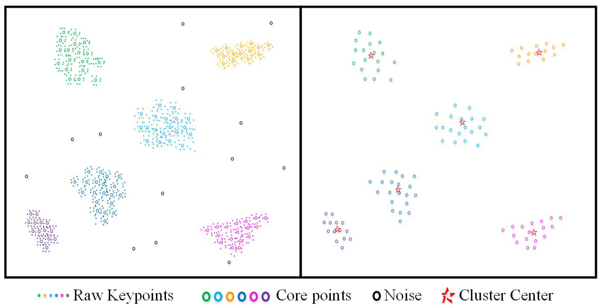
  • Strengthen the raw keypoints. The raw keypoints are chosen from initial ORB keypoints with a great Harris response [29].
  • Make the cluster smaller but more robust. Only use the core points to compute the cluster center as the initial representative points so that the points without sufficient neighbors will be ignored (Figure 5).
  • Find more precise representative points for the keyframes. Considering the keypoints which are closest to the cluster centers as the clustered keypoints of the keyframes (Figure 6).
  • Coarse-to-fine matching mechanism. Determine the searching areas in the current frame by brute-force matching [25] (Figure 7), then the clustered keypoints in the current frame matched with those in the keyframe will be found in the search patches by optical flow [30] (Figure 8).
In this way, only the feature points with the most enormous Harris response will be considered as clustered keypoints. As a result, we reduce hundreds or thousands of feature points to tens of much more stable clustered keypoints and avoid the influence of individual feature points that will disappear sometimes. The matched clustered keypoints after removing outliers are denoted as D C c * = { c 1 c * , c 2 c * , , c N c c * } and D C k * = { c 1 k * , c 2 k * , , c N c k * } . Where c i c * is the ith clustered keypoint in the current frame. The subscript C means clustered keypoints. In this paper, all of the superscript * indicates good matches between the current frame and the keyframe, N c is the number of good matched clustered keypoints, and the superscript c represents the current frame (k represents the keyframe).

3.3. Line Pairs from LK-ZNCC

Compared with points, lines provide more geometrical structure information of the environment [31]. In order to make the navigation system apply to various environments, such as natural scenes and structured scenarios, we couple point and line features in PLVC system. This section will show how the line segments are extracted, described, and matched.
The traditional line segment detection algorithms use Canny edge detector [32] and Hough transform (HT) [33]. Subsequently, there are many variants of HT [34,35,36,37] that propose to accelerate the runtime and enhance the precision. However, all of the HT-based algorithms generate infinitely long lines rather than line segments. Afterward, Grompone von Gioi et al. [38,39] present the line segment detector (LSD), which can produce precise line segments and reduce false detections. Whereas the runtime is still prohibitive, the white noises in the environment will influence the results. Akinlar and Topal [26,27] provide a fast and parameterless line segment detector, named EDlines in 2011, which can extract robust and accurate line segments in a pretty short time.
Describing and matching line segments are another two research focuses. The authors of [40] uses an affine invariant from two points and a line. This affine invariant matches lines if the point correspondences are already known. It is quite computationally expensive and has limited performance in low texture scenes due to the shortage of good point correspondences. Wang et al. [41] mention a kind of line descriptor called Mean-Standard deviation Line Descriptor (MSLD), which uses the appearance of pixel support regions. This method performs well for moderate image variations in textured scenes. Line Band Descriptor (LBD) [42] extracts line features by EDlines to form the line pairs. It overcomes segment fragmentation and geometric variation. Utilizing the local appearance of lines and their geometric attributes makes it robust to image transformations and perform efficiently and accurately. However, this algorithm runs pretty slow, especially in an environment with rich line features.
In this work, a set of line segments D L c = { l 1 c , l 2 c , , l N l c c } will be extracted in the current frame by EDlines, where N l c represents the number of line segments in this frame. Each line segment in D L c has three typical points, denoted as l i c { p s i c , p e i c , p m i c } = { ( x s i c , y s i c ) , ( x e i c , y e i c ) , ( x m i c , y m i c ) } where the subscript s represents start-point, e represents end-point and m represents midpoint. Since keyframes are selected from the current frame, there are D L k = { l 1 k , l 2 k , , l N l k k } for each keyframe accordingly.
Because of the small number of features, all-sided but simple characters are the best choices for describing the line segments so that accurate results can be computed in real-time. This means that the line segment descriptor needs to contain features of multiple dimensions such as local visual features in the neighborhood and the line segment’s length, position, and inclination. At the same time, the computational complexity should be kept as small as possible. In this paper, an algorithm named LK-ZNCC is proposed, which utilizes both photometric and geometric characters of line segments. It is worth noting that to reduce the computational complexity, we only select the three most representative points of the line segment to calculate its neighborhood similarity with the other line segment.
First, Lucas–Kanade optical flow [30] is exploited to track the midpoints p m j k in the current frame. Then, the neighborhoods of the tracked midpoints in the current frame are searched, and the accordingly, p m i c we found in these areas are determined to be the initially matched midpoints of line segments.
Subsequently, zero mean normalized cross correlation (ZNCC) [24] is employed to express the cost function (Equations (1)–(4)), which consists of the patch information of start-point, end-point, and midpoint of each initially matched line pairs.
S i j = S i j s + S i j e + S i j m 3
S i j s = I i s ( m , n ) I ¯ i s ( m , n ) I j s ( m , n ) I ¯ j s ( m , n ) I i s ( m , n ) I ¯ i s ( m , n ) 2 I j s ( m , n ) I ¯ j s ( m , n ) 2
S i j e = I i e ( m , n ) I ¯ i e ( m , n ) I j e ( m , n ) I ¯ j e ( m , n ) I i e ( m , n ) I ¯ i e ( m , n ) 2 I j e ( m , n ) I ¯ j e ( m , n ) 2
S i j m = I i m ( m , n ) I ¯ i m ( m , n ) I j m ( m , n ) I ¯ j m ( m , n ) I i m ( m , n ) I ¯ i ( m , n ) m 2 I j m ( m , n ) I ¯ j m ( m , n ) 2
where I = 1 m n m , n I ( m , n ) , S i j is the ZNCC score between ith segment line in the current frame and jth line segment in the keyframe; the superscripts s , e , m represent the patches of startpoint, end-point, midpoint; and I ( m , n ) is the intensity of the pixel in the mth row and nth column of the patch.
If the score of an initial line pairs satisfies Equation (5), they can be selected as candidate line pairs.
S i j T ZNCC ( T ZNCC = 0.85 ) ,
where T ZNCC is the minimum ZNCC score.
We have now matched all candidate line pairs between the keyframe and the current frame by photometric character. For the sake of simplicity, the above procedure of choosing candidate line pairs is named LK-ZNCC (shown in Figure 9).
However, a few outliers may exist in some exceptional cases due to the change of illumination and repeated textures. The geometric characters of line segments are applied to remove the wrong matches. Because we run the system in real-time, we suppose that the camera’s moving between the keyframe and the current frame is not too big. In this way, the candidate line pairs that meet the following conditions (Equation (6)) are the matched line segments finally, which are the line pairs denoted as D L c * = { l 1 c * , l 2 c * , , l N l c * } and D L k * = { l 1 k * , l 2 k * , , l N l k * } .
L l i c * L l j k * T Δ l d p m i c * , p m j k * = ( x m i c * x m j k * ) 2 + ( y m i c * y m j k * ) 2 T Δ l d
where N 1 is the number of the matched line pairs, L l i c * and L l j k * are the length of the matched line segments in the current frame and the keyframe. T Δ l is the maximum length difference of each line pair. d p m i c * , p m j k * is the distance between the midpoints of each line pair, and T Δ l d is the maximum value of it.
In addition, the midpoints of the line pairs are considered as the second part of point features, named line-based keypoints and denoted as D M c * = { p m 1 c * , p m 2 c * , , p m N l c * } and D M k * = { p m 1 k * , p m 2 k * , , p m N l k * } .

3.4. Computation of the Orientation Angle

3.4.1. Hierarchical Fusion of Point and Line Features

The hierarchical fusion contains two layers: the feature layer and the application layer. We create the matched line vectors for feature fusion by connecting every two keypoints from the previous point and line features as new features. Furthermore, for application fusion, the two kinds of orientation angles from line pairs and line vectors are loosely coupled to compute the final orientation angle of the camera.

Feature Fusion: Creating New Features

For each current frame and corresponding keyframe, Section 3.2 outputs clustered keypoints D C c * and D C k * , and Section 3.3 outputs line-based keypoints D M c * and D M k * . Both of the two parts constitute the global keypoints D P c * and D P k * (show in Figure 4):
D P c * = { D C c * , D M c * } = { p 1 c * , p 2 c * , , p N P c * } = { ( x 1 c * , y 1 c * ) , ( x 2 c * , y 2 c * ) , , ( x N P c * , y N P c * ) } D P k * = D C k * , D M k * = p 1 k * , p 2 k * , , p N P k * = x 1 k * , y 1 k * , x 2 k * , y 2 k * , , x N P k * , y N P k *
where N P represents the number of keypoints in our algorithm, N P = N c + N l .
Now it is easy to use two global keypoints of D P c * and two matched global keypoints of D P k * as the start-points and end-points to build two matched line vectors between the current frame and the keyframe. In this way, two sets of matched line vectors denoted as D V c * and D V k * can be obtained:
D V c * = v 1 c * , v 2 c * , , v N v c * D V k * = v 1 k * , v 2 k * , , v N v k *
where N v is the number of line vectors built by global keypoints:
N v = N P ( N P 1 ) 2
Therefore, line vectors D V c * and D V k * can derive two sets of inclination angles D θ v c * = { θ v 1 c * , θ v 2 c * , , θ v N v c * } in the current frame and D θ v k * = { θ v 1 k * , θ v 2 k * , , θ v N v k * } in the keyframe, where
θ v i c * = arctan y v i c * y v j c * x v i c * x v j c * θ v i k * = arctan y v i k * y v j k * x v i k * x v j k * i , j = 1 , 2 , . . . , N v 1 ; i j ; N v > T N l
where T N l is the minimum number of the matched line vectors.
Then, a group of orientation angle increments from global keypoints can be obtained as Equation (11):
Δ Ψ p i = D θ v c * D θ v k *
Another two sets of inclination angles D θ l c * = { θ l 1 c * , θ l 2 c * , , θ l N l c * } in the current frame and D θ l k * = { θ l 1 k * , θ l 2 k * , , θ l N l k * } in the keyframe can be computed by line pairs, where
θ l i c * = arctan y s i c * y e i c * x s i c * x e i c * θ l i k * = arctan y s i k * y e i k * x s i k * x e i k * i = 1 , 2 , . . . , N l ; i j ; N l > T N l
where N l is the number of the line pairs.
So the incremental orientation angle from line pairs are computed as Equation (13):
Δ Ψ l i = D θ l c * D θ l k *
The total computation process is shown in Figure 10.

Application Fusion: Loosely Couple Different Orientation Angles

Ideally, all of the Δ Ψ p i and Δ Ψ l i should be equal. However, because of the jitters of the UAV, illumination variation and dynamic objects in the environment, we consider that these orientation angle increments are uniform distribution with gaussian noises and some obvious outliers. At first, Δ Ψ p i * and Δ Ψ l i * are obtained from Δ Ψ p i and Δ Ψ l i after removing the outliers. Then, the final relative orientation angle will be estimated via the confidence coefficient of line vectors and line pairs (Equation (14)):
Δ Ψ = c o e v N v * Δ Ψ p i * N v * + c o e l N l * Δ Ψ l i * N l * c o e v = N v * N v * + N l * , c o e l = N l * N v * + N l *
where c o e v and c o e l are the confidence coefficient of line vectors and line pairs. Δ Ψ p i * and Δ Ψ l i * are the results of Δ Ψ p i and Δ Ψ l i after remove outliers. N v * and N l * are the size of Δ Ψ p i * and Δ Ψ l i * , the number of valid line vectors and line pairs.

3.4.2. Update the Keyframe

In order to reduce the error accumulation, the current frame is compared with the keyframe rather than the last frame. With the camera’s motion, it is crucial to update the keyframes. If the keyframe updates too frequently, the cumulative errors will be increased quickly. In contrast, the outcome is possible to be wrong and even fail since the matching of features maybe fails especially in the violent dynamic environment. Considering the above reasons, this paper designs two keyframe update conditions. The current frame will be set to a new keyframe when either of the conditions is satisfied:
N f T N k N P T N p , N l T N l
where N f is the number of interval frames between two keyframes; T N k is the maximum number of interval frames between two keyframes, and we set it to 5 in this article; T N p and T N l are the minimum number of the matched point features and matched line pairs, they are set to 0 in our experiments.

4. Results and Discussion

We perform real-world experiments to evaluate the proposed PLVC system. In this part, the matching result of global keypoints and line pairs will be displayed first. Then, we acquired some outdoor datasets in real-time flight on our UAV. And these datasets are used to compare the rotation estimation of PLVC and XSENS. Finally, some supplementary indoor experiments between PLVC, XSENS, and a high-precision magnetic compass were executed in our self-make platform to illustrate the influences of converge time, magnetic fields, and GPS for some present classic orientation angle estimation methods. The experiments were performed on a 2.3 GHz Intel(R) Core 4 processor with 16 GB of RAM. The average processing time of each frame is about 25 ms, and the camera frame rate is 30 Hz, which can realize real-time estimation. In conclusion, our PLVC can aid these methods well to evaluate the orientation angle when they are invalid at some time.

4.1. The Matching Result

This paper fuses a precise matched point and line features to make full use of the information in the environment and expand the usage of the algorithm. For the density-based clusters, since they are composed of the core points voted by sufficient neighbor raw keypoints, focusing on them can enhance the signal to noise ratio (SNR) by ignoring the influence of the sporadic points and dynamic objects. For line pairs, only those with high similarity in local appearance and geometric characters will be selected. This strict mechanism reduces the runtime deeply with enough accuracy and robustness. In feature layer fusion, the global keypoints including the clustered keypoints and the midpoints of line pairs are used to create line vectors. Figure 11 draws all of the global keypoints and line pairs in different scenes, which were captured by a downward-looking camera mounted on our UAV in our campus.
Note: The method of fusing point and line features proposed in this paper mainly aims to expand the applicable scenes from natural to structured. So different scenes in the experiments were more or less structured to verify the effection of line features.

4.2. Outdoor Datasets

In order to compare different sensors and algorithms that estimate the orientation angles of the UAVs, especially without enough translations, we built our own outdoor experiments datasets. Our experiments platform is a multirotor UAV, based on DJI M100, which mounts mounts a downward-looking monocular camera and a flight controller PIXHAWK (Figure 12).
The flight controller PIXHAWK records the flight data in real-time. It fuses IMU, GPS, magnetic compass, and barometer. Moreover, the IMU used in PIXHAWK includes three accelerometers, three gyroscopes, and two magnetometers. After a long period of use, it is regarded as a state-of-the-art product with accurate attitude estimations in the robotics field. The error margin of orientation angle estimation is 1.0 degrees. In conclusion, we use these flight data as the ground truth in this paper.
Considering the specific issue we intended to address, we made our UAV hover in the sky under the position model and rotated at different time and positions to acquire the data. The downward-looking monocular camera collected the figures while the PIXHAWK recorded the flight data. We have four kinds of experimental scenario settings:
  • ScSe: static UAV (camera) in static environment.
  • ScDe: static UAV (camera) in dynamic environment.
  • RcSe: rotating UAV (camera) in static environment.
  • RcDe: rotating UAV (camera) in dynamic environment.
Note: the static UAV means the attitude of it was intended to be stable. Nevertheless, there are some inevitable high-frequency jitters. While dynamic UAV means it just rotated in orientation angle. In a static environment, the scene watched by the camera was static while there were some moving objects in dynamic environments. Besides, the increments orientation angles of the UAV and the downward-looking camera mounted on the UAV are equal.

4.3. Outdoor Experiments

In these experiments, we evaluate the stability of PLVC when the UAV is hovering without rotation (ScSe and ScDe), validate the accuracy when the UAV is rotating (RcSe and RcDe), verify the robustness of the datasets that have dynamic objects (ScDe and RcDe). The mean values and covariances of the estimated orientation angle in different scenario settings and illumination are displayed in Table 1. In general, in the case of powerful and dim illumination, the accuracy of orientation angle estimation decreases because of the poor image quality, which directly affects the feature extraction. However, since this paper uses a small number of clustered point features and line segments instead of the original point features to calculate the orientation angle, the impact of poor image quality is reduced to some extent.
Note: In these experiments, we use the initial orientation angle ground-truth as Ψ 1 so that PLVC will output the absolute orientation angles.
Furthermore, parts of the comparison results of PLVC and ground-truth in similar illumination are shown in Figure 13. Figure 13a,b illustrate that PLVC is stable in some extent without too much drifts. Figure 13c,d show the state-of-the-art accuracy of PLVC even though there are dynamic objects in the scene.
In PLVC, we match the current frame with the keyframe and use several kinds of filters to handle the results. So even if the estimation has a big fault in some specific frames, it will come back to the correct scope (Figure 13c). The clustered keypoints and selected line pairs make the noises and dynamic objects omitted as well as shorten the runtime deeply. Even in the scenes with moving objects (Figure 13b,d), the errors only increase slightly (within 1 deg) and the precision is enough for UAV navigation. However, the dynamic object increases the dispersion degree of the error. That means error covariance increases more obviously because the cluster center points are slightly affected by the dynamic situation, and the stability of the center point is slightly reduced.

4.4. Supplementary Indoor Experiments

In order to illustrate the performance of PLVC on plug and play, anti-magnetic interference, and working in a GPS-denied environment, we also compare it with other excellent traditional sensors, such as XSENS, magnetic compass, and GPS-denied multi-sensors system. Here are some introduction of these sensors and the reason why we choose them in our supplementary experiments:
  • XSENS: A kind of high-accuracy IMU whose product model is MTi-300. Although the orientation angle is unobservable for IMU, XSENS is considered as an excellent state estimation sensor because of the fused magnetic compass and the precise state estimation algorithm. The estimation accuracy of the orientation angle can reach 1 degree. However, it needs a few minutes to set up the sensors and converge the fusing algorithm inside when it powers on.
  • Magnetic Compass: A high-precision magnetic compass DCM260B whose estimation error is 0.8 degree. Though this magnetic compass is seen as precise as the ground truth, the changes of the surrounding magnetic field influence it.
  • GPS-denied multi-sensors system: As presented before, PIXHAWK works well with GPS and the flight data is considered as ground truth. Nevertheless, how the multi-sensors system performs in GPS-denied cases needs to be certified.
To account for the above analysis, we set converge time, changes of magnetic fields and GPS-denied or not as three experiment conditions needed to be controlled. Then, three sets supplementary experiments were carried out online using a single axis pan-tilt. There is a downward-looking monocular camera, a high-precise IMU XSENS and magnetic compass mounted on the single axis pan-tilt to estimate the orientation angle of it (Figure 14). Besides, these three sets of experiments have different conditions and targets:
  • Converge Time: These three sensors are compared just after power on and three minutes later to test the converge time for XSENS.
  • Changes of Magnetic Fields: The sensors are used in the metallic and non-metallic environment to test the influence of magnetic field for a magnetic compass.
  • GPS-denied or Not: The magnetic compass is replaced by the flight controller we used in outdoor experiments, but the GPS is invalid in the internal environment. So, the influence of GPS can be displayed.

4.4.1. Testing the Converge Time

These experiments are executed in a non-metallic environment (including pan-tilt and frame). The pan-tilt mounts a camera running PLVC, XSENS and a magnetic compass DCM260B. Here, the magnetic compass data was considered as ground truth because in this case, no magnetic field changes interfere with the working of the magnetic compass. These three sensors were compared just after being powered on and three minutes later to test the converge time for XSENS. In order to show the converging process, these experiments were only run on the static body in the static scene (ScSe), so the ground truth is 0 degrees. Figure 15 confirms the truth that XSENS does need a long time to converge. It performs well once finishing converging. However, this condition limits the usage of XSENS when it is expected to be used just after being powered on in some situations. In contrast, our PLVC does not need to wait for this period of time and can be used plug-and-play. Besides, the magnetic compass can be thought of as ground truth when there is no distribution from magnetic field changes.

4.4.2. Testing the Changes of Magnetic Fields

Magnetic compasses are always used in UAVs to estimate the orientation angles. However, there is a crucial flaw that the magnetic compass is very susceptible to being disturbed by the surrounding magnetic field. To illustrate this influence factor, we use two single-axis pan-tilts made from different materials for the rotating body in static environments (RcSe). The rotating body is driven by a programmed steering gear. The first single-axis pan-tilt is metallic and fixed on a metal frame. While the second one is made of a non-metallic material and fixed in a non-metallic environment. A downward-looking monocular camera running our PLVC, XSENS and a high-precise magnetic compass is mounted on both of the pan-tilts (Figure 14), and the orientation angles are collected after adequate convergence time, so the data of XSENS, the error margin of which is 1.0 degrees, can be seen as the ground truth according to Section 4.4.1 with little drift that can be ignored.
Note: The rotation angles of XSENS are equal to the control directions for the steering gear.
Figure 16 demonstrates that different orientation angles are obtained with the same experiments because of the different materials of the platform. A magnetic compass is more demanding on the environment and can easily be interfered with by magnetic field changes, limiting its usage on UAVs. In comparison, this issue will not happen on PLVC.

4.4.3. Testing the Effect of GPS

The flight controller is necessary for UAVs. PIXHAWK fuses traditional navigation sensors, such as GPS, three sets of IMUs, a magnetic compass, and a barometer. It has been proven to have excellent performance on state estimation and control. However, can flight control still work in a GPS-denied environment?
In this part, the magnetic compass in the non-metallic pan-tilt before is replaced by the flight controller PIXHAWK. Then, we run PLVC, XSENS, and PIXHAWK on the rotated pan-tilt after adequate converge time in a static environment (RcSe). So the orientation angle of XSENS can be seen as the ground truth the error margin is 1.0 degrees. The comparison is shown in Figure 17. The flight data from the flight controller is drifting seriously without GPS signal. From this perspective, using a vision method to aid traditional sensors in estimating the orientation angle is significant.

5. Conclusions

In this paper, we proposed an uncalibrated visual compass named PLVC, which uses remote sensing images to estimate the orientation angle of a UAV. Because the scene in the image can be seen as a plane, the algorithm uses both appearance and geometry information of 2D point and line features in the 3D scene. The proposed visual compass algorithm can assist the current traditional sensors well, especially when the UAV is in some particular environments, like GPS-denied, inadequate translation, and rich magnetic field changes. While traditional navigation systems and current visual compass algorithms need various sensors, most of the sensors need to be calibrated. Our methods performs well even though the illumination changed and dynamic objects appeared. It is plug-and-play and robust to noises, but uses a low-cost monocular camera without any calibrations and alignments, suitable for long-focal length cameras in UAVs. In the future, a camera could fuse with other sensors to estimate the absolute 3D attitude angles directly, rather than relative orientation angle.

6. Patents

  • Yu Zhang, Ying Liu, Ping Li. Zhejiang University. A directional downward-looking compass based on the visual and inertial information: China, ZL2018101196741, 27 May 2020.
  • Yu Zhang, Ying Liu, Ping Li. Zhejiang University. A downward-looking visual compass based on the point and line features: China, ZL2018106233944, 30 April 2021.

Author Contributions

Conceptualization, Y.L.; methodology, Y.L.; software, Y.L.; validation, Y.L.; formal analysis, Y.L. and J.T.; investigation, Y.L. and J.T.; data curation, Y.L. and J.T.; writing—original draft preparation, Y.L., J.T. and D.K.; writing—review and editing, Y.Z., Y.L., J.T. and D.K.; visualization, Y.L.; supervision, Y.Z. and P.L.; project administration, Y.Z.; funding acquisition, Y.Z. All authors have read and agreed to the published version of the manuscript.

Funding

This work was supported by the National Key Research and Development Program of China under Grant 2021ZD0201400, the National Natural Science Foundation of China (Grant No.62088101, 61673341), the Project of State Key Laboratory of Industrial Control Technology, Zhejiang University, China (No.ICT2021A10), the Fundamental Research Funds for the Central Universities (No.2021FZZX003-01-06), Double First Class University Plan (CN).

Institutional Review Board Statement

Not applicable.

Informed Consent Statement

Not applicable.

Data Availability Statement

Not applicable.

Conflicts of Interest

The authors declare no conflict of interest. The funders had no role in the design of the study; in the collection, analyses, or interpretation of data; in the writing of the manuscript, or in the decision to publish the results.

References

  1. Karantanellis, E.; Marinos, V.; Vassilakis, E.; Christaras, B. Object-based analysis using unmanned aerial vehicles (UAVs) for site-specific landslide assessment. Remote Sens. 2020, 12, 1711. [Google Scholar] [CrossRef]
  2. Xu, J.; Zhu, T.; Bian, H. Review on gps attitude determination. J. Nav. Univ. Eng. 2003, 36, 17–22. [Google Scholar]
  3. Li, Y.; Zahran, S.; Zhuang, Y.; Gao, Z.; Luo, Y.; He, Z.; Pei, L.; Chen, R.; El-Sheimy, N. IMU/magnetometer/barometer/mass-flow sensor integrated indoor quadrotor UAV localization with robust velocity updates. Remote Sens. 2019, 11, 838. [Google Scholar] [CrossRef] [Green Version]
  4. Mariottini, G.L.; Scheggi, S.; Morbidi, F.; Prattichizzo, D. An accurate and robust visual-compass algorithm for robot-mounted omnidirectional cameras. Robot. Auton. Syst. 2012, 60, 1179–1190. [Google Scholar] [CrossRef]
  5. Liu, Y.; Zhang, Y.; Li, P.; Xu, B. Uncalibrated downward-looking UAV visual compass based on clustered point features. Sci. China Inf. Sci. 2019, 62, 199202. [Google Scholar] [CrossRef] [Green Version]
  6. Klein, G.; Murray, D. Parallel tracking and mapping for small AR workspaces. In Proceedings of the 2007 6th IEEE and ACM International Symposium on Mixed and Augmented Reality, Nara, Japan, 13–16 November 2007; pp. 225–234. [Google Scholar]
  7. Mur-Artal, R.; Montiel, J.M.M.; Tardos, J.D. ORB-SLAM: A versatile and accurate monocular SLAM system. IEEE Trans. Robot. 2015, 31, 1147–1163. [Google Scholar] [CrossRef] [Green Version]
  8. Engel, J.; Koltun, V.; Cremers, D. Direct sparse odometry. IEEE Trans. Pattern Anal. Mach. Intell. 2017, 40, 611–625. [Google Scholar] [CrossRef]
  9. Teed, Z.; Deng, J. Droid-slam: Deep visual slam for monocular, stereo, and rgb-d cameras. arXiv 2021, arXiv:2108.10869. [Google Scholar]
  10. Xu, W.; Zhong, S.; Zhang, W.; Wang, J.; Yan, L. A New Orientation Estimation Method Based on Rotation Invariant Gradient for Feature Points. IEEE Geosci. Remote Sens. Lett. 2020, 18, 791–795. [Google Scholar] [CrossRef]
  11. Mariottini, G.L.; Scheggi, S.; Morbidi, F.; Prattichizzo, D. A robust uncalibrated visual compass algorithm from paracatadioptric line images. In First Workshop on Omnidirectional Robot Vision, Lecture Notes in Computer Science; Springer: Berlin/Heidelberg, Germany, 2009. [Google Scholar]
  12. Morbidi, F.; Caron, G. Phase correlation for dense visual compass from omnidirectional camera-robot images. IEEE Robot. Autom. Lett. 2017, 2, 688–695. [Google Scholar] [CrossRef] [Green Version]
  13. Montiel, J.M.; Davison, A.J. A visual compass based on SLAM. In Proceedings of the 2006 IEEE International Conference on Robotics and Automation, Orlando, FL, USA, 15–19 May 2006; ICRA 2006. pp. 1917–1922. [Google Scholar]
  14. Pajdla, T.; Hlaváč, V. Zero phase representation of panoramic images for image based localization. In Proceedings of the International Conference on Computer Analysis of Images and Patterns, Ljubljana, Slovenia, 1–3 September 1999; Springer: Berlin/Heidelberg, Germany, 1999; pp. 550–557. [Google Scholar]
  15. Menegatti, E.; Maeda, T.; Ishiguro, H. Image-based memory for robot navigation using properties of omnidirectional images. Robot. Auton. Syst. 2004, 47, 251–267. [Google Scholar] [CrossRef] [Green Version]
  16. Stürzl, W.; Mallot, H.A. Efficient visual homing based on Fourier transformed panoramic images. Robot. Auton. Syst. 2006, 54, 300–313. [Google Scholar] [CrossRef]
  17. Differt, D. Real-time rotational image registration. In Proceedings of the 2017 18th International Conference on Advanced Robotics (ICAR), Hong Kong, China, 10–12 July 2017; pp. 1–6. [Google Scholar]
  18. Makadia, A.; Geyer, C.; Sastry, S.; Daniilidis, K. Radon-based structure from motion without correspondences. In Proceedings of the 2005 IEEE Computer Society Conference on Computer Vision and Pattern Recognition (CVPR’05), San Diego, CA, USA, 20–25 June 2005; Volume 1, pp. 796–803. [Google Scholar]
  19. Sturm, J.; Visser, A. An appearance-based visual compass for mobile robots. Robot. Auton. Syst. 2009, 57, 536–545. [Google Scholar] [CrossRef] [Green Version]
  20. Lv, W.; Kang, Y.; Zhao, Y.B. FVC: A novel nonmagnetic compass. IEEE Trans. Ind. Electron. 2018, 66, 7810–7820. [Google Scholar] [CrossRef]
  21. Kim, P.; Li, H.; Joo, K. Quasi-globally Optimal and Real-time Visual Compass in Manhattan Structured Environments. IEEE Robot. Autom. Lett. 2022, 7, 2613–2620. [Google Scholar] [CrossRef]
  22. Sabnis, A.; Vachhani, L. A multiple camera based visual compass for a mobile robot in dynamic environment. In Proceedings of the 2013 IEEE International Conference on Control Applications (CCA), Hyderabad, India, 28–30 August 2013; pp. 611–616. [Google Scholar]
  23. Sturzl, W. A lightweight single-camera polarization compass with covariance estimation. In Proceedings of the IEEE International Conference on Computer Vision, Venice, Italy, 22–29 October 2017; pp. 5353–5361. [Google Scholar]
  24. Di Stefano, L.; Mattoccia, S. Fast template matching using bounded partial correlation. Mach. Vis. Appl. 2003, 13, 213–221. [Google Scholar]
  25. Rublee, E.; Rabaud, V.; Konolige, K.; Bradski, G. ORB: An efficient alternative to SIFT or SURF. In Proceedings of the 2011 International Conference on Computer Vision, Washington, DC, USA, 6–13 November 2011; pp. 2564–2571. [Google Scholar]
  26. Akinlar, C.; Topal, C. Edlines: Real-time line segment detection by edge drawing (ed). In Proceedings of the 2011 18th IEEE International Conference on Image Processing, Brussels, Belgium, 11–14 September 2011; pp. 2837–2840. [Google Scholar]
  27. Akinlar, C.; Topal, C. EDLines: A real-time line segment detector with a false detection control. Pattern Recognit. Lett. 2011, 32, 1633–1642. [Google Scholar] [CrossRef]
  28. Ester, M.; Kriegel, H.P.; Sander, J.; Xu, X. A density-based algorithm for discovering clusters in large spatial databases with noise. KDD 1996, 96, 226–231. [Google Scholar]
  29. Harris, C.G.; Stephens, M.J. A combined corner and edge detector. Alvey Vis. Conf. 1988, 2, 147–151. [Google Scholar]
  30. Lucas, B.D.; Kanade, T. An iterative image registration technique with an application to stereo vision. In Proceedings of the 7th International Joint Conference on Artificial Intelligence, IJCAI ’81, Vancouver, BC, Canada, 24–28 August 1981. [Google Scholar]
  31. He, Y.; Zhao, J.; Guo, Y.; He, W.; Yuan, K. Pl-vio: Tightly-coupled monocular visual–inertial odometry using point and line features. Sensors 2018, 18, 1159. [Google Scholar] [CrossRef] [Green Version]
  32. Canny, J. A computational approach to edge detection. IEEE Trans. Pattern Anal. Mach. Intell. 1986, PAMI-8, 679–698. [Google Scholar] [CrossRef]
  33. Hough, P.V. Method and Means for Recognizing Complex Patterns. U.S. Patent 3,069,654, 18 December 1962. [Google Scholar]
  34. Xu, L.; Oja, E.; Kultanen, P. A new curve detection method: Randomized Hough transform (RHT). Pattern Recognit. Lett. 1990, 11, 331–338. [Google Scholar] [CrossRef]
  35. Kiryati, N.; Eldar, Y.; Bruckstein, A.M. A probabilistic Hough transform. Pattern Recognit. 1991, 24, 303–316. [Google Scholar] [CrossRef]
  36. Galambos, C.; Kittler, J.; Matas, J. Gradient based progressive probabilistic Hough transform. IEEE Proc.-Vis. Image Signal Process. 2001, 148, 158–165. [Google Scholar] [CrossRef] [Green Version]
  37. Fernandes, L.A.; Oliveira, M.M. Real-time line detection through an improved Hough transform voting scheme. Pattern Recognit. 2008, 41, 299–314. [Google Scholar] [CrossRef]
  38. Von Gioi, R.G.; Jakubowicz, J.; Morel, J.M.; Randall, G. LSD: A line segment detector. Image Process. Online 2012, 2, 35–55. [Google Scholar] [CrossRef] [Green Version]
  39. Von Gioi, R.G.; Jakubowicz, J.; Morel, J.M.; Randall, G. LSD: A fast line segment detector with a false detection control. IEEE Trans. Pattern Anal. Mach. Intell. 2008, 32, 722–732. [Google Scholar] [CrossRef]
  40. Fan, B.; Wu, F.; Hu, Z. Line matching leveraged by point correspondences. In Proceedings of the 2010 IEEE Computer Society Conference on Computer Vision and Pattern Recognition, San Francisco, CA, USA, 13–18 June 2010; pp. 390–397. [Google Scholar]
  41. Wang, Z.; Wu, F.; Hu, Z. MSLD: A robust descriptor for line matching. Pattern Recognit. 2009, 42, 941–953. [Google Scholar] [CrossRef]
  42. Zhang, L.; Koch, R. An efficient and robust line segment matching approach based on LBD descriptor and pairwise geometric consistency. J. Vis. Commun. Image Represent. 2013, 24, 794–805. [Google Scholar] [CrossRef]
Figure 1. The main idea of PLVC, the orientation angles can be decoupled from attitude angles for estimation and the translation is not related to its computation. Figure 1(1) shows the original 3D line l c in the world frame. When the camera rotates around z c axis, l c ’s direction will change to l c (Figure 1(2)). In general, the rotation axis of the camera is not parallel with the z c axis, which means not only the yaw angle, but the roll and pitch angle will change. In this case, the projected line l i can be derived by decoupling the three attitude angles (Figure 1(3)), and the increment yaw angle of the camera equals the included angle of l i and l i ( Δ Ψ in Figure 1(4)), which is also the intersection angle of l c and l c in the plane x c o c y c (Figure 1(3)).
Remotesensing 14 01430 g001
Figure 2. The computation strategy of the relative orientation angle in this paper. Note that if the rotation angle is denoted as Δ Ψ , then Δ Ψ = Δ Ψ 1 = Δ Ψ 2 in theory.
Remotesensing 14 01430 g002
Figure 3. The pipeline of PLVC.
Remotesensing 14 01430 g003
Figure 4. The schematic diagram of the PLVC algorithm. The colorful points are the raw keypoints, and different colors represent different clusters.
Remotesensing 14 01430 g004
Figure 5. Cluster the raw ORB keypoints and compute the cluster centers only by core points.
Remotesensing 14 01430 g005
Figure 6. Choose precise cluster center for the keyframe, named as clustered keypoint.
Remotesensing 14 01430 g006
Figure 7. Match clustered keypoints in the keyframe with cluster centers (compute from positions) in the current frame to determine the searching areas for the clustered keypoints in the current frame.
Remotesensing 14 01430 g007
Figure 8. Determine the clustered keypoints in the current frame.
Remotesensing 14 01430 g008
Figure 9. The process of matching line segments.
Remotesensing 14 01430 g009
Figure 10. Compute orientation angle increments. Line vectors are built from global keypoints (consist of clustered keypoints and midpoints of line pairs).
Remotesensing 14 01430 g010
Figure 11. The matching results of clustered keypoints and line pairs in outdoor experiments. In the orientation angle estimation, the confidence of line features is high in the first scene because it is structured, while the confidence of point features is high in the second scene since it is partly natural.
Remotesensing 14 01430 g011
Figure 12. The UAV used in outdoor experiments.
Remotesensing 14 01430 g012
Figure 13. The comparison results of PLVC and groundtruth.
Remotesensing 14 01430 g013
Figure 14. The single axis pan-tilt used in the supplementary online experiments. There is a monocular camera (bottom), a compass (middle) and a XSENS (top) mounted on the self-made platform. (a) is the metallic platform and (b) is the non-metallic platform.
Remotesensing 14 01430 g014
Figure 15. The comparison of magnetic compass/PLVC/XSENS with static camera in static environment (ScSe). The left picture shows the result of the output collected as soon as the program is started. The right one reports the result of the output collected after waiting for nearly 3 min. Here the ground truth is 0 degree.
Remotesensing 14 01430 g015
Figure 16. The comparison of PLVC/XSENS/magnetic compass in different platforms with rotating camera in a static environment (RcSe) after converging, so the data from XSENS can be seen as ground truth. The left image shows the comparison result in the metallic platform (with the distribution of magnetic fields). The right one shows the comparison result in the non-metallic platform (without distribution of magnetic fields).
Remotesensing 14 01430 g016
Figure 17. The comparison of PLVC/XSENS/PIXHAWK (without GPS) with rotating camera in a static indoor environment (RcSe) after converge, so the data from XSENS can be seen as ground truth. The left image displays the increments of orientation angles. The right one demonstrates the comparison result of the orientation angle without GPS. The estimation results with GPS are shown in Figure 13.
Remotesensing 14 01430 g017
Table 1. The estimation error of PLVC in different experimental scenario settings and illuminations.
Scenario SettingsIlluminationTest1Test2Test3
Mean (deg)Cov (deg)Mean (deg)Cov (deg)Mean (deg)Cov (deg)
ScSe+++−0.16630.23270.3634−0.33150.08350.5367
++−0.11490.3189−0.00340.52673.949 × 10 15 0.1750
+0.15670.16400.43370.17500.56470.3762
ScDe+++−0.50730.38090.9909−0.54511.0718−0.1028
++−0.11250.15260.6468−0.0238−3.99 × 10 14 −0.1484
+−0.46430.37661.0183−0.00681.0718−0.1028
RcSe+++−0.10700.72951.83630.63391.60500.6339
++0.93650.7783−0.25052.45790.07281.0686
+−0.66741.0272−0.27601.06861.75731.4529
RcDe+++0.15670.1640−0.36260.6875−0.25060.6875
++−1.42921.3539−0.23690.9934−0.13300.9934
+−0.10710.8869−1.04270.7606−0.01930.7606
Note: The experimental scenario settings include different UAV motions and scenes, which are described in Section 4.2. We performed three sets of experiments with three different illumination conditions for each scenario setting. For illumination, “+++” means strong, “++” is medium, and “+” is dark. We collected these datasets at noon, afternoon, and nightfall. “Mean” is the mean error between PLVC and ground truth. “Cov” is the covariance error between PLVC and ground-truth. Since ground truth error is 1°, we may state that nearly all errors listed in the table are not significant.
Publisher’s Note: MDPI stays neutral with regard to jurisdictional claims in published maps and institutional affiliations.

