
The Self-Supervised Spectral–Spatial Vision Transformer Network for Accurate Prediction of Wheat Nitrogen Status from UAV Imagery


 ,
,
Abstract
:1. Introduction
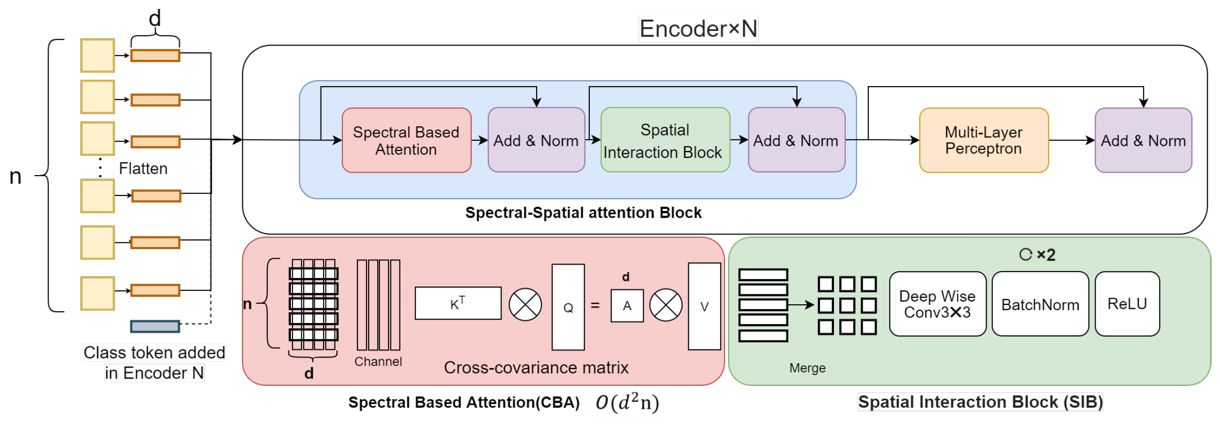
- A novel spectral–spatial attention-based vision transformer is proposed, in which both the spectral and spatial information are considered. A Spectral Attention Block (SAB) is proposed to learn spectral-wise features such as colour information. Meanwhile, a Spatial Interact (SIB) is introduced after SBA to learn corresponding spatial information.
- A local-to-global self-supervised learning (SSL) method is proposed to pretrain the model on the unlabelled images to resolve the data-hungry paradigm in DL model training and improve the model’s generalization performance on independent data.
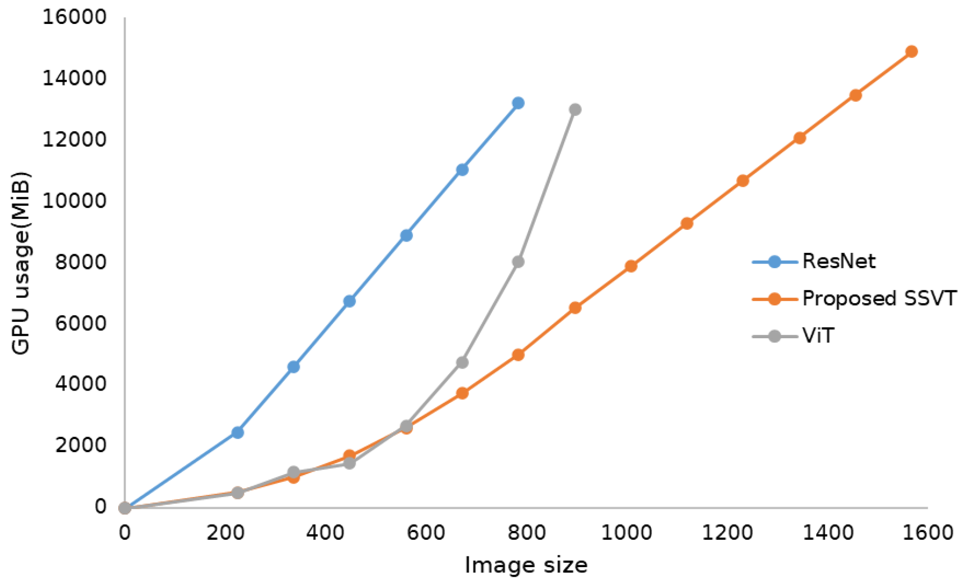
- A linear computational complexity is achieved using the cross-covariance matrix instead of the original gram matrix operation in the attention block. It changes the complexity of the transformer layer from quadratic to linear, which makes it possible for the model to handle large size images.
2. Related Work
2.1. Non-Destructive Crop N Estimation Methods
2.2. Vision Transformer
2.3. Self-Supervised Learning (SSL)
3. Method and Materials
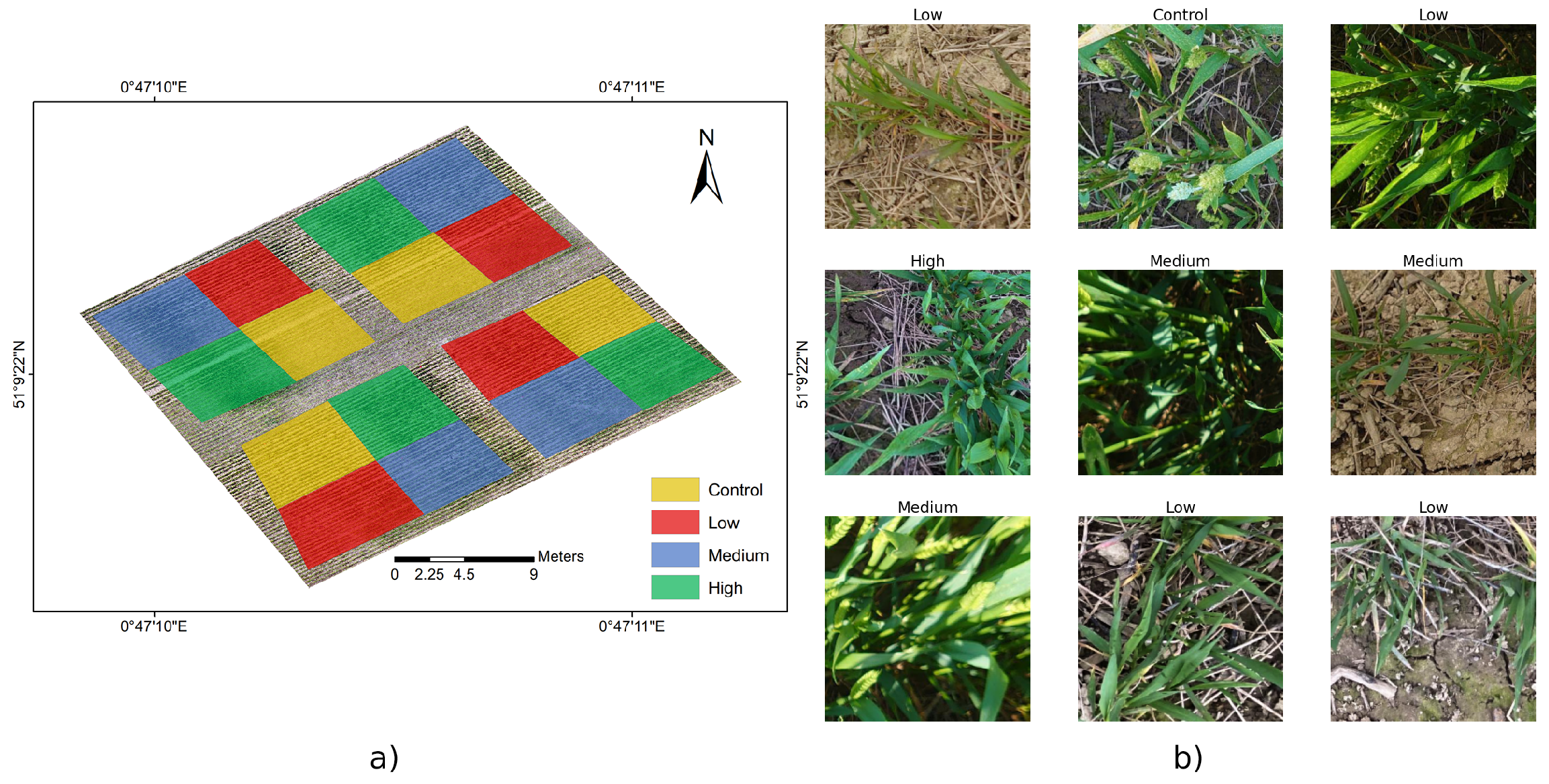
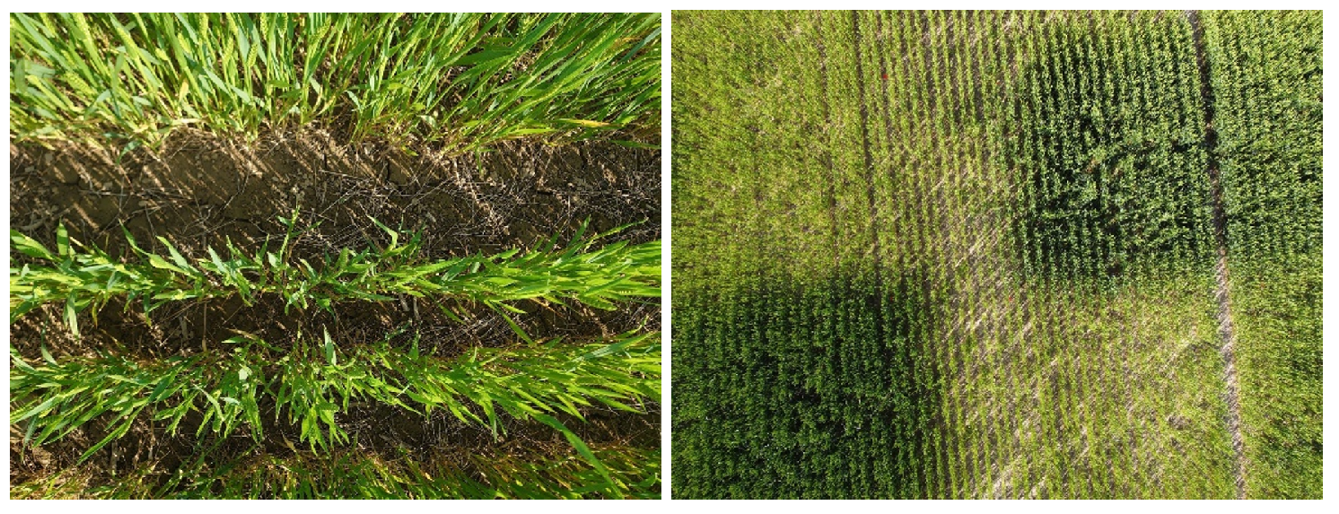
3.1. Dataset Description
3.2. Method
3.2.1. Spectral–Spatial attention Vision Transformer (SSVT)
- As shown in previous research [11], spectral information plays a vital role in determining nitrogen status at leaf and canopy scales. In this work, the spectral-based attention block is proposed to learn spectral-wise features such as colour information.
- To learn the spatial information, a spatial interaction block is introduced after the spectral-based attention block.
- To address the quadratic computing complexity of the ViT, the covariance matrix is used to replace the gram matrix, which can help reduce computational complexity from the quadratic complexity () to linear complexity () where n represents the number of input patches.
Spectral–Spatial Attention Block
Spectral Based Attention (SBA)
Spatial Interaction Block (SIB)
Multilayer Perceptron (MLP)
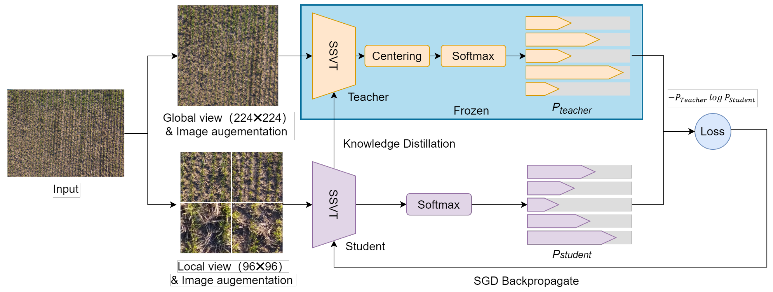
3.3. Local-to-Global Self-Supervised Learning
| Algorithm 1 Local-to-Global SSL algorithm |
Require:
|
3.4. Model Evaluation
3.4.1. Experimental Design
Performance Evaluation of SSVT for Automated Crop N Prediction
Ablation Study
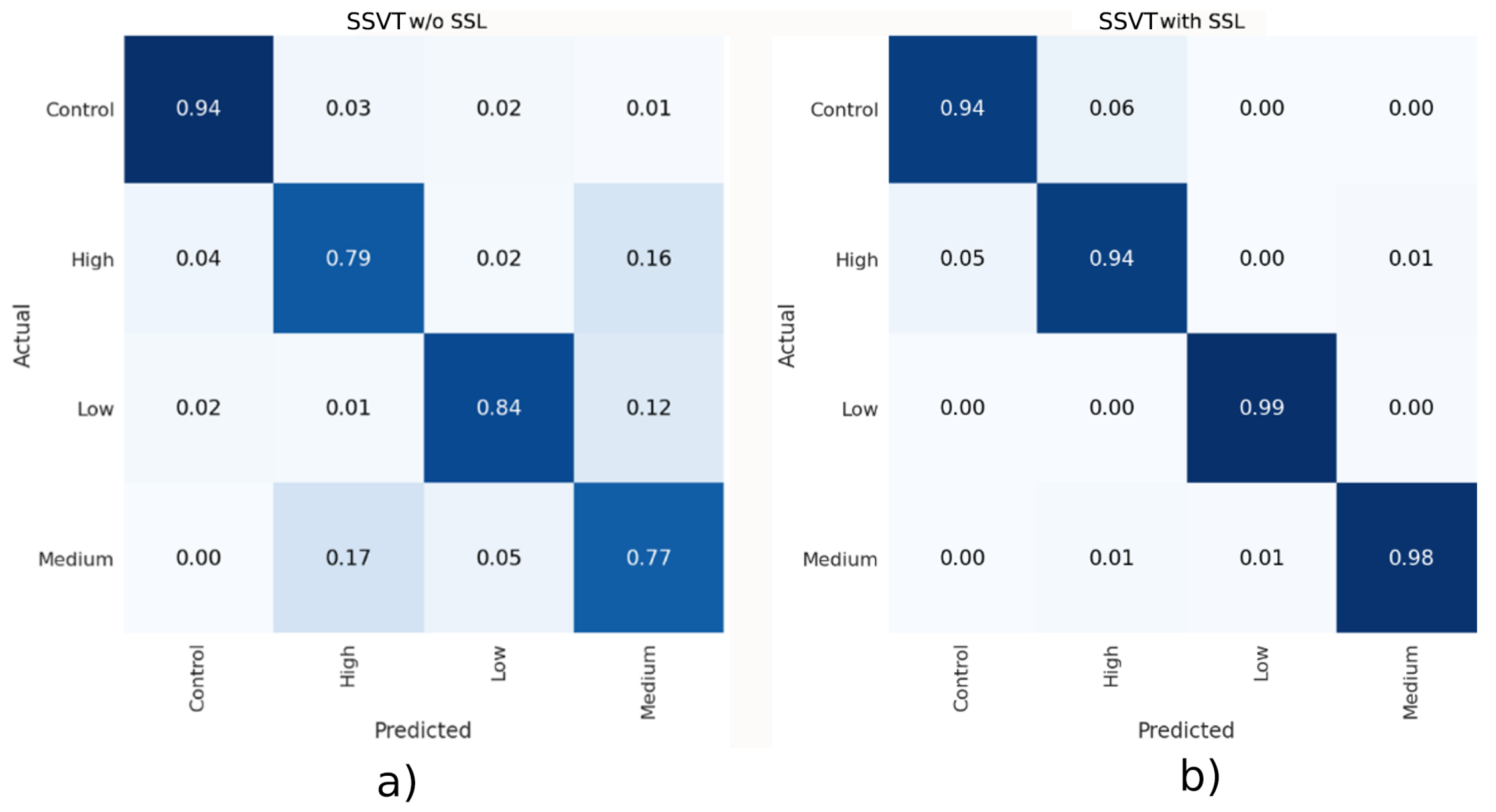
The Performance of the Proposed SSVT with and without SSL
The Impact of the Spectral–Spatial Attention Block
Evaluation of the Generalizability of the Proposed Model Using Independent Drone Datasets
3.4.2. Evaluation Metrics
3.4.3. Experimental Configuration
4. Result
4.1. Performance Evaluation of SSVT for Automated Crop N Prediction
4.2. Ablation Study
4.2.1. The Performance of the Proposed SSVT with and without SSL
4.2.2. The Impact of the Spectral–Spatial Attention Block
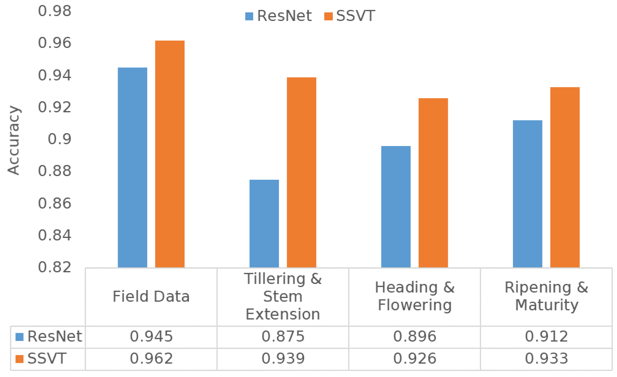
4.3. Evaluation of the Generalizability of the Proposed Model Using Independent Datasets
5. Discussion
5.1. Performance of SSVT for Automated Crop N Prediction
5.2. Prospects and Future Work
6. Conclusions
Author Contributions
Funding
Institutional Review Board Statement
Informed Consent Statement
Acknowledgments
Conflicts of Interest
References
- FAO. World Fertilizer Trends and Outlook to 2020: Summary Report; FAO: Rome, Italy, 2017. [Google Scholar]
- Good, A. Toward nitrogen-fixing plants. Science 2018, 359, 869–870. [Google Scholar] [CrossRef]
- Berger, K.; Verrelst, J.; Féret, J.B.; Wang, Z.; Wocher, M.; Strathmann, M.; Danner, M.; Mauser, W.; Hank, T. Crop nitrogen monitoring: Recent progress and principal developments in the context of imaging spectroscopy missions. Remote Sens. Environ. 2020, 242, 111758. [Google Scholar] [CrossRef]
- Wang, D.; Xu, Z.; Zhao, J.; Wang, Y.; Yu, Z. Excessive nitrogen application decreases grain yield and increases nitrogen loss in a wheat–soil system. Acta Agric. Scand. Sect. B-Soil Plant Sci. 2011, 61, 681–692. [Google Scholar] [CrossRef]
- Knoema. Wheat Area Harvested. 2021. Available online: https://knoema.com//atlas/topics/Agriculture/Crops-Production-Area-Harvested/Wheat-area-harvested (accessed on 8 August 2021).
- Benitez Ramirez, M. Monitoring Nitrogen Levels in the Cotton Canopy Using Real-Time Active-Illumination Spectral Sensing. Master’s Thesis, University of Tennessee, Knoxville, TN, USA, 2010. [Google Scholar]
- Wang, J.; Shen, C.; Liu, N.; Jin, X.; Fan, X.; Dong, C.; Xu, Y. Non-destructive evaluation of the leaf nitrogen concentration by in-field visible/near-infrared spectroscopy in pear orchards. Sensors 2017, 17, 538. [Google Scholar] [CrossRef] [Green Version]
- Imani, M.; Ghassemian, H. An overview on spectral and spatial information fusion for hyperspectral image classification: Current trends and challenges. Inf. Fusion 2020, 59, 59–83. [Google Scholar] [CrossRef]
- Johnson, D.M. An assessment of pre-and within-season remotely sensed variables for forecasting corn and soybean yields in the United States. Remote Sens. Environ. 2014, 141, 116–128. [Google Scholar] [CrossRef]
- Fitzgerald, G.; Rodriguez, D.; O’Leary, G. Measuring and predicting canopy nitrogen nutrition in wheat using a spectral index—The canopy chlorophyll content index (CCCI). Field Crops Res. 2010, 116, 318–324. [Google Scholar] [CrossRef]
- Chlingaryan, A.; Sukkarieh, S.; Whelan, B. Machine learning approaches for crop yield prediction and nitrogen status estimation in precision agriculture: A review. Comput. Electron. Agric. 2018, 151, 61–69. [Google Scholar] [CrossRef]
- Jordan, M.I.; Mitchell, T.M. Machine learning: Trends, perspectives, and prospects. Science 2015, 349, 255–260. [Google Scholar] [CrossRef]
- Shi, P.; Wang, Y.; Xu, J.; Zhao, Y.; Yang, B.; Yuan, Z.; Sun, Q. Rice nitrogen nutrition estimation with RGB images and machine learning methods. Comput. Electron. Agric. 2021, 180, 105860. [Google Scholar] [CrossRef]
- Qiu, Z.; Ma, F.; Li, Z.; Xu, X.; Ge, H.; Du, C. Estimation of nitrogen nutrition index in rice from UAV RGB images coupled with machine learning algorithms. Comput. Electron. Agric. 2021, 189, 106421. [Google Scholar] [CrossRef]
- Zhang, X.; Han, L.; Han, L.; Zhu, L. How well do deep learning-based methods for land cover classification and object detection perform on high resolution remote sensing imagery? Remote Sens. 2020, 12, 417. [Google Scholar] [CrossRef] [Green Version]
- Roth, L.; Streit, B. Predicting cover crop biomass by lightweight UAS-based RGB and NIR photography: An applied photogrammetric approach. Precis. Agric. 2018, 19, 93–114. [Google Scholar] [CrossRef] [Green Version]
- Alom, M.Z.; Hasan, M.; Yakopcic, C.; Taha, T.M.; Asari, V.K. Improved inception-residual convolutional neural network for object recognition. Neural Comput. Appl. 2018. [Google Scholar] [CrossRef] [Green Version]
- Nanni, L.; Ghidoni, S.; Brahnam, S. Handcrafted vs. non-handcrafted features for computer vision classification. Pattern Recognit. 2017, 71, 158–172. [Google Scholar] [CrossRef]
- Lewis, K.P.; Espineli, J.D. Classification And Detection of Nutritional Deficiencies in Coffee Plants Using Image Processing And Convolutional Neural Network (CNN). Int. J. Sci. Technol. Res. 2020, 9, 6. [Google Scholar]
- Sethy, P.K.; Barpanda, N.K.; Rath, A.K.; Behera, S.K. Nitrogen Deficiency Prediction of Rice Crop Based on Convolutional Neural Network. J. Ambient. Intell. Humaniz. Comput. 2020, 11, 5703–5711. [Google Scholar] [CrossRef]
- Tran, T.T.; Choi, J.W.; Le, T.T.H.; Kim, J.W. A Comparative Study of Deep CNN in Forecasting and Classifying the Macronutrient Deficiencies on Development of Tomato Plant. Appl. Sci. 2019, 9, 1601. [Google Scholar] [CrossRef] [Green Version]
- Wolf, T.; Debut, L.; Sanh, V.; Chaumond, J.; Delangue, C.; Moi, A.; Cistac, P.; Rault, T.; Louf, R.; Funtowicz, M.; et al. Transformers: State-of-the-Art Natural Language Processing. In Proceedings of the 2020 Conference on Empirical Methods in Natural Language Processing: System Demonstrations, Online, 16–20 November 2020; Association for Computational Linguistic, 2020; pp. 38–45. Available online: https://aclanthology.org/2020.emnlp-demos.6/ (accessed on 12 May 2021).
- Scharf, P.; Schmidt, J.; Kitchen, N.; Sudduth, K.; Hong, S.; Lory, J.; Davis, J. Remote sensing for nitrogen management. J. Soil Water Conserv. 2002, 57, 518–524. [Google Scholar]
- Hunt, E.R., Jr.; Doraiswamy, P.C.; McMurtrey, J.E.; Daughtry, C.S.; Perry, E.M.; Akhmedov, B. A visible band index for remote sensing leaf chlorophyll content at the canopy scale. Int. J. Appl. Earth Obs. Geoinf. 2013, 21, 103–112. [Google Scholar] [CrossRef] [Green Version]
- Solovchenko, A.; Merzlyak, M. Screening of visible and UV radiation as a photoprotective mechanism in plants. Russ. J. Plant Physiol. 2008, 55, 719–737. [Google Scholar] [CrossRef]
- Yang, W.H.; Peng, S.; Huang, J.; Sanico, A.L.; Buresh, R.J.; Witt, C. Using leaf color charts to estimate leaf nitrogen status of rice. Agron. J. 2003, 95, 212–217. [Google Scholar] [CrossRef]
- Baret, F.; Hagolle, O.; Geiger, B.; Bicheron, P.; Miras, B.; Huc, M.; Berthelot, B.; Niño, F.; Weiss, M.; Samain, O.; et al. LAI, fAPAR and fCover CYCLOPES global products derived from VEGETATION: Part 1: Principles of the algorithm. Remote Sens. Environ. 2007, 110, 275–286. [Google Scholar] [CrossRef] [Green Version]
- Hank, T.B.; Berger, K.; Bach, H.; Clevers, J.G.; Gitelson, A.; Zarco-Tejada, P.; Mauser, W. Spaceborne imaging spectroscopy for sustainable agriculture: Contributions and challenges. Surv. Geophys. 2019, 40, 515–551. [Google Scholar] [CrossRef] [Green Version]
- Lu, B.; He, Y. Evaluating empirical regression, machine learning, and radiative transfer modelling for estimating vegetation chlorophyll content using bi-seasonal hyperspectral images. Remote Sens. 2019, 11, 1979. [Google Scholar] [CrossRef] [Green Version]
- Wocher, M.; Berger, K.; Danner, M.; Mauser, W.; Hank, T. RTM-based dynamic absorption integrals for the retrieval of biochemical vegetation traits. Int. J. Appl. Earth Obs. Geoinf. 2020, 93, 102219. [Google Scholar] [CrossRef]
- Verhoef, W. Light scattering by leaf layers with application to canopy reflectance modeling: The SAIL model. Remote Sens. Environ. 1984, 16, 125–141. [Google Scholar] [CrossRef] [Green Version]
- Wang, Z.; Skidmore, A.K.; Darvishzadeh, R.; Heiden, U.; Heurich, M.; Wang, T. Leaf nitrogen content indirectly estimated by leaf traits derived from the PROSPECT model. IEEE J. Sel. Top. Appl. Earth Obs. Remote Sens. 2015, 8, 3172–3182. [Google Scholar] [CrossRef]
- Padilla, F.M.; Gallardo, M.; Peña-Fleitas, M.T.; De Souza, R.; Thompson, R.B. Proximal optical sensors for nitrogen management of vegetable crops: A review. Sensors 2018, 18, 2083. [Google Scholar] [CrossRef] [PubMed] [Green Version]
- Clevers, J.G.; Gitelson, A.A. Remote estimation of crop and grass chlorophyll and nitrogen content using red-edge bands on Sentinel-2 and-3. Int. J. Appl. Earth Obs. Geoinf. 2013, 23, 344–351. [Google Scholar] [CrossRef]
- Afandi, S.D.; Herdiyeni, Y.; Prasetyo, L.B.; Hasbi, W.; Arai, K.; Okumura, H. Nitrogen content estimation of rice crop based on near infrared (NIR) reflectance using artificial neural network (ANN). Procedia Environ. Sci. 2016, 33, 63–69. [Google Scholar] [CrossRef] [Green Version]
- Pagola, M.; Ortiz, R.; Irigoyen, I.; Bustince, H.; Barrenechea, E.; Aparicio-Tejo, P.; Lamsfus, C.; Lasa, B. New method to assess barley nitrogen nutrition status based on image colour analysis: Comparison with SPAD-502. Comput. Electron. Agric. 2009, 65, 213–218. [Google Scholar] [CrossRef]
- Zha, H.; Miao, Y.; Wang, T.; Li, Y.; Zhang, J.; Sun, W.; Feng, Z.; Kusnierek, K. Improving unmanned aerial vehicle remote sensing-based rice nitrogen nutrition index prediction with machine learning. Remote Sens. 2020, 12, 215. [Google Scholar] [CrossRef] [Green Version]
- Mehra, L.K.; Cowger, C.; Gross, K.; Ojiambo, P.S. Predicting pre-planting risk of Stagonospora nodorum blotch in winter wheat using machine learning models. Front. Plant Sci. 2016, 7, 390. [Google Scholar] [CrossRef]
- Lee, K.J.; Lee, B.W. Estimating canopy cover from color digital camera image of rice field. J. Crop Sci. Biotechnol. 2011, 14, 151–155. [Google Scholar] [CrossRef]
- Li, Y.; Chen, D.; Walker, C.N.; Angus, J.F. Estimating the nitrogen status of crops using a digital camera. Field Crops Res. 2010, 118, 221–227. [Google Scholar] [CrossRef]
- Zhao, B.; Zhang, Y.; Duan, A.; Liu, Z.; Xiao, J.; Liu, Z.; Qin, A.; Ning, D.; Li, S.; Ata-Ul-Karim, S.T. Estimating the Growth Indices and Nitrogen Status Based on Color Digital Image Analysis During Early Growth Period of Winter Wheat. Front. Plant Sci. 2021, 12, 502. [Google Scholar] [CrossRef]
- Azimi, S.; Kaur, T.; Gandhi, T.K. A deep learning approach to measure stress level in plants due to Nitrogen deficiency. Measurement 2021, 173, 108650. [Google Scholar] [CrossRef]
- Lee, S.H.; Chan, C.S.; Mayo, S.J.; Remagnino, P. How deep learning extracts and learns leaf features for plant classification. Pattern Recognit. 2017, 71, 1–13. [Google Scholar] [CrossRef] [Green Version]
- Islam, M.A.; Jia, S.; Bruce, N.D.B. How Much Position Information Do Convolutional Neural Networks Encode? arXiv 2020, arXiv:2001.08248. [Google Scholar]
- Vaswani, A.; Shazeer, N.; Parmar, N.; Uszkoreit, J.; Jones, L.; Gomez, A.N.; Kaiser, L.; Polosukhin, I. Attention Is All You Need. arXiv 2017, arXiv:1706.03762. [Google Scholar]
- Dong, Y.; Cordonnier, J.B.; Loukas, A. Attention is Not All You Need: Pure Attention Loses Rank Doubly Exponentially with Depth. arXiv 2021, arXiv:2103.03404. [Google Scholar]
- Touvron, H.; Cord, M.; Douze, M.; Massa, F.; Sablayrolles, A.; Jégou, H. Training data-efficient image transformers & distillation through attention. arXiv 2021, arXiv:2012.12877. [Google Scholar]
- Liu, X.; Zhang, F.; Hou, Z.; Mian, L.; Wang, Z.; Zhang, J.; Tang, J. Self-supervised learning: Generative or contrastive. IEEE Trans. Knowl. Data Eng. 2021, 1. [Google Scholar] [CrossRef]
- Goodfellow, I.J.; Pouget-Abadie, J.; Mirza, M.; Xu, B.; Warde-Farley, D.; Ozair, S.; Courville, A.; Bengio, Y. Generative Adversarial Networks. arXiv 2014, arXiv:1406.2661. [Google Scholar] [CrossRef]
- Hadsell, R.; Chopra, S.; LeCun, Y. Dimensionality Reduction by Learning an Invariant Mapping. In Proceedings of the 2006 IEEE Computer Society Conference on Computer Vision and Pattern Recognition (CVPR’06), New York, NY, USA, 17–22 June 2006; 2006; Volume 2, pp. 1735–1742. [Google Scholar]
- Bromley, J.; Bentz, J.W.; Bottou, L.; Guyon, I.; LeCun, Y.; Moore, C.; Säckinger, E.; Shah, R. Signature verification using a “siamese” time delay neural network. Int. J. Pattern Recognit. Artif. Intell. 1993, 7, 669–688. [Google Scholar] [CrossRef] [Green Version]
- Grill, J.B.; Strub, F.; Altché, F.; Tallec, C.; Richemond, P.H.; Buchatskaya, E.; Doersch, C.; Pires, B.A.; Guo, Z.D.; Azar, M.G.; et al. Bootstrap your own latent: A new approach to self-supervised Learning. arXiv 2020, arXiv:2006.07733. [Google Scholar]
- Caron, M.; Misra, I.; Mairal, J.; Goyal, P.; Bojanowski, P.; Joulin, A. Unsupervised Learning of Visual Features by Contrasting Cluster Assignments. arXiv 2021, arXiv:2006.09882. [Google Scholar]
- He, K.; Fan, H.; Wu, Y.; Xie, S.; Girshick, R. Momentum Contrast for Unsupervised Visual Representation Learning. In Proceedings of the IEEE/CVF Conference on Computer Vision and Pattern Recognition (CVPR 2020), Seattle, WA, USA, 14–19 June 2020; pp. 9729–9738. [Google Scholar]
- Chen, T.; Kornblith, S.; Norouzi, M.; Hinton, G. A Simple Framework for Contrastive Learning of Visual Representations. arXiv 2020, arXiv:2002.05709. [Google Scholar]
- OpenDroneMap/ODM. A Command Line Toolkit to Generate Maps, Point Clouds, 3D Models and DEMs from Drone, Balloon or Kite Images. 2020. Available online: https://github.com/OpenDroneMap/ODM (accessed on 26 January 2022).
- El-Nouby, A.; Touvron, H.; Caron, M.; Bojanowski, P.; Douze, M.; Joulin, A.; Laptev, I.; Neverova, N.; Synnaeve, G.; Verbeek, J.; et al. XCiT: Cross-Covariance Image Transformers. arXiv 2021, arXiv:2106.09681. [Google Scholar]
- Ba, J.L.; Kiros, J.R.; Hinton, G.E. Layer Normalization. arXiv 2016, arXiv:1607.06450. [Google Scholar]
- Howard, A.G.; Zhu, M.; Chen, B.; Kalenichenko, D.; Wang, W.; Weyand, T.; Andreetto, M.; Adam, H. MobileNets: Efficient Convolutional Neural Networks for Mobile Vision Applications. arXiv 2017, arXiv:1704.04861. [Google Scholar]
- Zhang, L.; Song, J.; Gao, A.; Chen, J.; Bao, C.; Ma, K. Be Your Own Teacher: Improve the Performance of Convolutional Neural Networks via Self Distillation. In Proceedings of the 2019 IEEE/CVF International Conference on Computer Vision (ICCV), Seoul, Korea, 27–28 October 2019; pp. 3712–3721. [Google Scholar]
- He, K.; Zhang, X.; Ren, S.; Sun, J. Deep residual learning for image recognition. In Proceedings of the IEEE Conference on Computer Vision and Pattern Recognition, Las Vegas, NV, USA, 26 June–1 July 2016; pp. 770–778. [Google Scholar]
- Tan, M.; Le, Q. Efficientnet: Rethinking model scaling for convolutional neural networks. In Proceedings of the International Conference on Machine Learning (PMLR), Long Beach, CA, USA, 9–15 June 2019; pp. 6105–6114. [Google Scholar]
- Radosavovic, I.; Kosaraju, R.P.; Girshick, R.; He, K.; Dollár, P. Designing Network Design Spaces. arXiv 2020, arXiv:2003.13678. [Google Scholar]
- Tan, M.; Le, Q.V. EfficientNetV2: Smaller Models and Faster Training. arXiv 2021, arXiv:2104.00298. [Google Scholar]
- Zhang, H.; Cisse, M.; Dauphin, Y.N.; Lopez-Paz, D. mixup: Beyond empirical risk minimization. arXiv 2017, arXiv:1710.09412. [Google Scholar]
- Müller, R.; Kornblith, S.; Hinton, G. When does label smoothing help? arXiv 2019, arXiv:1906.02629. [Google Scholar]
- Buslaev, A.; Iglovikov, V.I.; Khvedchenya, E.; Parinov, A.; Druzhinin, M.; Kalinin, A.A. Albumentations: Fast and Flexible Image Augmentations. Information 2020, 11, 125. [Google Scholar] [CrossRef] [Green Version]
- Putra, B.T.W.; Soni, P. Improving nitrogen assessment with an RGB camera across uncertain natural light from above-canopy measurements. Precis. Agric. 2020, 21, 147–159. [Google Scholar] [CrossRef]
- Shorten, C.; Khoshgoftaar, T.M. A survey on image data augmentation for deep learning. J. Big Data 2019, 6, 60. [Google Scholar] [CrossRef]
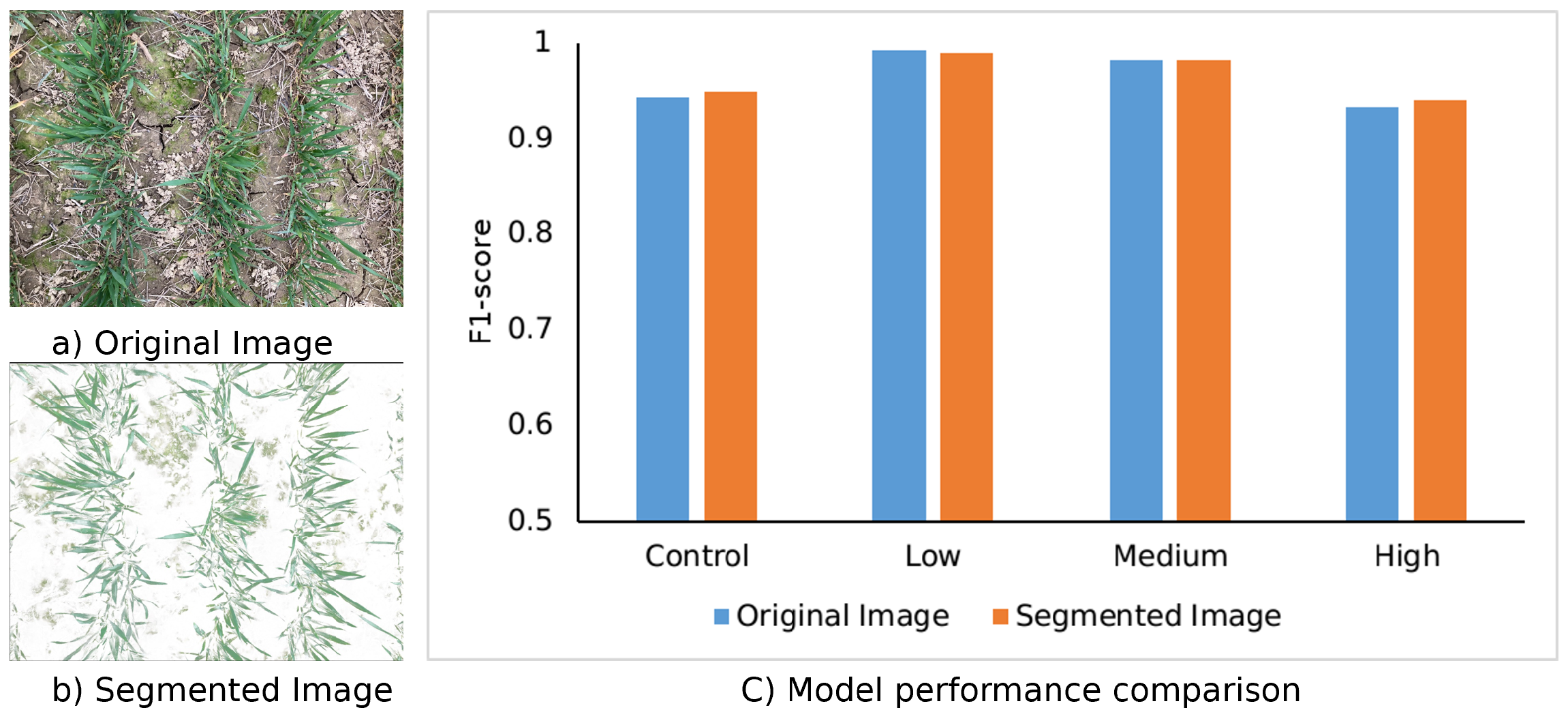
- Hernández-Hernández, J.L.; García-Mateos, G.; González-Esquiva, J.; Escarabajal-Henarejos, D.; Ruiz-Canales, A.; Molina-Martínez, J.M. Optimal color space selection method for plant/soil segmentation in agriculture. Comput. Electron. Agric. 2016, 122, 124–132. [Google Scholar] [CrossRef]
- Dyson, J.; Mancini, A.; Frontoni, E.; Zingaretti, P. Deep learning for soil and crop segmentation from remotely sensed data. Remote Sens. 2019, 11, 1859. [Google Scholar] [CrossRef] [Green Version]
- Zhang, H.Y.; Ren, X.X.; Zhou, Y.; Wu, Y.P.; He, L.; Heng, Y.R.; Feng, W.; Wang, C.Y. Remotely assessing photosynthetic nitrogen use efficiency with in situ hyperspectral remote sensing in winter wheat. Eur. J. Agron. 2018, 101, 90–100. [Google Scholar] [CrossRef]
- Liu, H.; Zhu, H.; Li, Z.; Yang, G. Quantitative analysis and hyperspectral remote sensing of the nitrogen nutrition index in winter wheat. Int. J. Remote Sens. 2020, 41, 858–881. [Google Scholar] [CrossRef]
- Cui, R.; Liu, Y.; Fu, J. Estimation of winter wheat leaf nitrogen accumulation using machine learning algorithm and visible spectral. Guang Pu Xue Yu Guang Pu Fen Xi = Guang Pu 2016, 36, 1837–1842. [Google Scholar] [PubMed]
- Shah, S.H.; Angel, Y.; Houborg, R.; Ali, S.; McCabe, M.F. A random forest machine learning approach for the retrieval of leaf chlorophyll content in wheat. Remote Sens. 2019, 11, 920. [Google Scholar] [CrossRef] [Green Version]
- AHDB. Nutrient Management Guide (RB209)|AHDB. 2021. Available online: https://ahdb.org.uk/nutrient-management-guide-rb209 (accessed on 26 January 2022).


| Growing Stage | Date | Field Image Collection | Drone |
|---|---|---|---|
| Tillering & Stem Extension | 21-March | 160 | ✓ |
| 2-April | 163 | ✓ | |
| 9-April | 177 | ✓ | |
| Heading & Flowering | 6-May | 166 | ✓ |
| 14-May | 177 | ✓ | |
| 24-May | 175 | ✓ | |
| Ripening & Maturity | 7-June | 177 | ✓ |
| 22-June | 177 | ✓ | |
| 28-June | 175 | ✓ |
| Parameter | Value |
|---|---|
| Camera-lens | Auto |
| Cameras | DJI MAVIC pro |
| Matcher algorithm | Fast Library for Approximate Nearest Neighbors |
| Gps-accuracy | 10 m |
| Fast-orthophoto | True |
| Orthophoto-resolution | 0.1 and 0.3 cm |
| Cloud based geotiff | True |
| Model | Patch Size | Layer | Dimension | Param (M) |
|---|---|---|---|---|
| ViT | 8 | 12 | 384 | 21.67 |
| SSVT | 8 | 12 | 384 | 25.87 |
| Image Size | ||||
| Types of N Treatments | Control | Low | Medium | High |
| Precision | 0.949 | 0.992 | 0.985 | 0.923 |
| Recall | 0.936 | 0.992 | 0.98 | 0.941 |
| F1-score | 0.943 | 0.992 | 0.982 | 0.932 |
| Accuracy | 0.962 | |||
| Image Size | ||||
| Precision | 0.973 | 0.991 | 0.982 | 0.917 |
| Recall | 0.924 | 0.989 | 0.981 | 0.964 |
| F1-score | 0.948 | 0.99 | 0.982 | 0.94 |
| Accuracy | 0.965 | |||
| Param (M) | GFLOPs (GMac) | Accuracy (%) | |
|---|---|---|---|
| ResNet_50 | 23.52 | 4.12 | 0.945 |
| EfficientNet_B5 | 28.35 | 2.4 | 0.95 |
| RegNetY-4.0G | 20.6 | 4.1 | 0.951 |
| EfficientNetv2_small | 20.18 | 2.87 | 0.949 |
| ViT | 21.67 | 4.24 | 0.944 |
| SSVT | 25.87 | 4.71 | 0.962 |
| Model | SSVT w/o SSL | |||
|---|---|---|---|---|
| Types of N Treatments | Control | Low | Medium | High |
| Precision | 0.937 | 0.898 | 0.738 | 0.784 |
| Recall | 0.939 | 0.844 | 0.774 | 0.789 |
| F1-score | 0.938 | 0.87 | 0.756 | 0.787 |
| Accuracy | 0.836 | |||
| Model | ViT | |||
| Types of N Treatments | Control | Low | Medium | High |
| Precisio | 0.925 | 0.956 | 0.931 | 0.969 |
| Recall | 0.994 | 0.975 | 0.944 | 0.865 |
| F1-score | 0.959 | 0.965 | 0.938 | 0.914 |
| Accuracy | 0.944 | |||
| Model | SSVT | |||
| Precision | 0.949 | 0.992 | 0.985 | 0.923 |
| Recall | 0.936 | 0.992 | 0.98 | 0.941 |
| F1-score | 0.943 | 0.992 | 0.982 | 0.932 |
| Accuracy | 0.962 | |||
| References | Modality | Objective | Accuracy |
|---|---|---|---|
| [72] | (VI)-based methods | Nitrogen use efficiency | 0.85 |
| [73] | (VI)-based methods | Nitrogen nutrition index | 0.86 |
| [74] | Artificial Neural Network (ANN)/Support Vector Regression (SVR) | Leaf nitrogen accumulation | 0.86 |
| [75] | Random Forest | Chlorophyll content | 0.89 |
| [37] | Random Forest | Nitrogen nutrition index | 0.94 |
| Proposed method | SSVT | Nitrogen status | 0.96 |
Publisher’s Note: MDPI stays neutral with regard to jurisdictional claims in published maps and institutional affiliations. |
© 2022 by the authors. Licensee MDPI, Basel, Switzerland. This article is an open access article distributed under the terms and conditions of the Creative Commons Attribution (CC BY) license (https://creativecommons.org/licenses/by/4.0/).
Share and Cite
Zhang, X.; Han, L.; Sobeih, T.; Lappin, L.; Lee, M.A.; Howard, A.; Kisdi, A. The Self-Supervised Spectral–Spatial Vision Transformer Network for Accurate Prediction of Wheat Nitrogen Status from UAV Imagery. Remote Sens. 2022, 14, 1400. https://doi.org/10.3390/rs14061400
Zhang X, Han L, Sobeih T, Lappin L, Lee MA, Howard A, Kisdi A. The Self-Supervised Spectral–Spatial Vision Transformer Network for Accurate Prediction of Wheat Nitrogen Status from UAV Imagery. Remote Sensing. 2022; 14(6):1400. https://doi.org/10.3390/rs14061400
Chicago/Turabian StyleZhang, Xin, Liangxiu Han, Tam Sobeih, Lewis Lappin, Mark A. Lee, Andew Howard, and Aron Kisdi. 2022. "The Self-Supervised Spectral–Spatial Vision Transformer Network for Accurate Prediction of Wheat Nitrogen Status from UAV Imagery" Remote Sensing 14, no. 6: 1400. https://doi.org/10.3390/rs14061400
APA StyleZhang, X., Han, L., Sobeih, T., Lappin, L., Lee, M. A., Howard, A., & Kisdi, A. (2022). The Self-Supervised Spectral–Spatial Vision Transformer Network for Accurate Prediction of Wheat Nitrogen Status from UAV Imagery. Remote Sensing, 14(6), 1400. https://doi.org/10.3390/rs14061400