Article

Early Detection of Dendroctonus valens Infestation with Machine Learning Algorithms Based on Hyperspectral Reflectance

1
Beijing Key Laboratory for Forest Pest Control, Beijing Forestry University, Beijing 100083, China
2
School of Ecology and Nature Conservation, Beijing Forestry University, Beijing 100083, China
3
Sino-French Joint Laboratory for Invasive Forest Pests in Eurasia, Beijing Forestry University—French National Research Institute for Agriculture, Food and Environment (INRAE), Beijing 100083, China
*
Author to whom correspondence should be addressed.
Remote Sens. 2022, 14(6), 1373; https://doi.org/10.3390/rs14061373
Submission received: 30 January 2022 / Revised: 7 March 2022 / Accepted: 10 March 2022 / Published: 11 March 2022
(This article belongs to the Topic Big Data and Artificial Intelligence)

Abstract

:
The red turpentine beetle (Dendroctonus valens LeConte) has caused severe ecological and economic losses since its invasion into China. It gradually spreads northeast, resulting in many Chinese pine (Pinus tabuliformis Carr.) deaths. Early detection of D. valens infestation (i.e., at the green attack stage) is the basis of control measures to prevent its outbreak and spread. This study examined the changes in spectral reflectance after initial attacking of D. valens. We also explored the possibility of detecting early D. valens infestation based on spectral vegetation indices and machine learning algorithms. The spectral reflectance of infested trees was significantly different from healthy trees (p < 0.05), and there was an obvious decrease in the near-infrared region (760–1386 nm; p < 0.01). Spectral vegetation indices were input into three machine learning classifiers; the classification accuracy was 72.5–80%, while the sensitivity was 65–85%. Several spectral vegetation indices (DID, CUR, TBSI, DDn2, D735, SR1, NSMI, RNIR•CRI550 and RVSI) were sensitive indicators for the early detection of D. valens damage. Our results demonstrate that remote sensing technology could be successfully applied to early detect D. valens infestation and clarify the sensitive spectral regions and vegetation indices, which has important implications for early detection based on unmanned airborne vehicle and satellite data.

1. Introduction

The red turpentine beetle (RTB; Dendroctonus valens LeConte) is an important invasive pest in China. Since it was discovered in Shanxi Province in 1998, it has spread rapidly and caused severe mortality of pine trees, resulting in serious ecological and economic losses [1]. By the end of 2004, RTB occurred in an area of more than 500,000 hectares and killed more than 6 million pine trees, resulting in direct economic losses of CNY 684 million and ecological losses of CNY 8.1 billion [2]. In recent years, the infestation area has spread northeast and reached Inner Mongolia and Liaoning provinces in 2017. A simulation study showed that under future climate conditions, the potential distribution of RTB will expand to a higher latitude, and the suitable degree of survival will rise in most areas [3], which means that the range and intensity of RTB outbreaks would increase as regional and global temperatures increase. Therefore, it is crucial to implement control measures to prevent RTB epidemics.
In its native origin—North and Central America—RTB is a secondary pest attacking weak and dying pines. After being introduced to China, RTBs prefer to attack Chinese pine (Pinus tabuliformis Carr.) with a large diameter at breast height and can kill healthy pines [4]. RTB usually has one generation per year in most regions in China, while in some regions, it has either two generations a year or two generations in 3 years, depending on local climate and site conditions [5,6]. This beetle overwinters as larvae or adults in roots, and the adults begin to disperse in late spring. There is overlapping of generations, and the adults can be seen in the field until October. Adults massively attack the lower stem of pines and lay eggs under the bark. Subsequently, the larvae hatch and feed on the pine phloem and cambium, forming common galleries. The feeding behavior of larvae and the presence of associated fungi cut off the nutrient and water transport of infested pines [1]. After being colonized, the hosts undergo a discoloration process. Similar to mountain pine beetle (MPB) and spruce bark beetle (SBB), the process can be divided into three stages according to the crown color, termed green, red and gray attack [7,8]. During the green attack (GA) stage, the needles of infested pine are still green and alive, and the crown does not show visually observable symptoms [9]. Our investigation (unpublished data) found that the GA stage is the early stage, in which the new generation of RTB is still within the host tree. Once the infested pine crowns show obvious discoloration, most RTBs have already left the pines (Figure 1). Therefore, disposing of attacked pines before the emergence and migration of new generations, i.e., at the GA stage, is a crucial strategy to control the spread and avoid the outbreak of RTB, which requires timely and accurate information.
The traditional method to identify RTB-infested trees is to look for pitch tubes and boring dust during ground surveys. Although the information provided by ground surveys is the most precise, it is laborious, time-consuming and difficult to cover large areas, which may result in missing the best time for the prevention of an outbreak. The developments of remote sensing and data processing technology would provide opportunities to monitor and assess the health status of forests in large areas. Several reviews summarized the application cases or potential of remote sensing for forest health monitoring from different perspectives [10,11,12,13,14]. To date, many studies used multispectral satellite data to detect and monitor bark beetle damages. For example, single-date or multi-date medium-resolution satellite data (e.g., Landsat and Sentinel-2 data) were used to detect infestation plots and monitor the dynamics of bark beetle outbreaks in Europe and North America [15,16,17,18,19]. A few studies assessed the ability of Sentinel-2 or Landsat data for early detection [20,21,22,23]. However, their low spatial resolution only enables the detection of infested stands, whereas there are different attack stages simultaneously present in infested forests. High-spatial-resolution satellite images (e.g., IKONOS, GeoEye-1, QuickBird and WorldView-2) were used to detect tree mortality (i.e., red and gray attack stages) caused by bark beetles and achieved high accuracies [24,25,26]. Zhan et al. [9] evaluated the ability of Gaofen-2 to detect tree mortality caused by RTB with an overall accuracy of 77.7%. However, the trees they identified were in the last two attack stages, which are hysteretic and insufficient for preventing the spread of bark beetles by salvage logging. Immitzer et al. [27] and Mullen [28] used WorldView-2 imagery to detect the early stage of SBB infestation in Norway and MPB infestation in ponderosa pine forest, respectively. In their results, the classification accuracy of the “green attack” was about 70%, and the high within-class variances overlapped the spectral differences between classes. Therefore, it is still problematic to detect the GA stage of bark beetle infestation using multispectral satellite data because of the limited spatial and spectral resolution.
In recent years, the potential of hyperspectral data for the early detection of stress has attracted attention. Some studies attempted to detect early infestation of bark beetles by using airborne hyperspectral data but, unfortunately, were not able to effectively distinguish between GA and healthy trees [29,30,31,32,33,34]. Compared with the canopy level, the spectrum at the leaf level is less disturbed by background noise and has a higher spectral resolution, which can capture finer spectral responses and provide a better understanding of spectral changes under stress. Several studies used ground-based hyperspectral sensors in the field or laboratory to detect changes in spectral properties at the leaf level. Ahern [35] found three important spectral regions and a red shift of the red edge at the early stage of MPB infestation in lodgepole pine trees. He noted that the shoulder of the NIR plateau was the most promising for early detection, and there was an interaction between needle age and attack status. However, Reichmuth et al. [36] concluded different results from a ring-barking experiment on Norway spruce and multi-temporal laboratory needle hyperspectral data, in which they found that the visible spectral region was more important than the NIR region for detecting stress, and the spectral data between different age classes were significantly similar. Cheng et al. [37] used continuous wavelet analysis to detect the spectral responses of MPB-infested and girdled trees. Their results show that the needle water content of infested trees decreased and the spectral features located between 950 and 1390 nm were sensitive to the GA stage, whereas both needle water and chlorophyll content of girdled trees were significantly different from the healthy trees, and the spectral features used to distinguish girdled and healthy trees were located between 1550 and 2370 nm. Foster et al. [8] confirmed that the SWIR region is an important region for detecting the early stage of Dendroctonus rufipennis infestation. Abdullah et al. [38] measured the mean spectral reflectance and foliar biochemical (i.e., chlorophyll and nitrogen content) between healthy and SBB-infested Norway spruce, and significant differences were observed, with the differences of reflectance being most distinct in the region from 730 to 1370 nm. Several studies also used hyperspectral data for other species and diseases (e.g., Sirex noctilio [39], pine shoot beetles [40] and pine wilt disease [41]) and screened for different spectral features that could be used for early detection. According to previous studies, spectral responses and important features for early detection may vary with host, stress factors and observation scales. To date, the spectral changes in the early stage of RTB infestation have not been studied.
Here, we evaluated the potential of hyperspectral data for the early detection of RTB infestation. The specific objectives of the study were (1) to compare the differences of spectral reflectance between the GA stage and healthy trees, (2) to establish classifiers combining machine learning (ML) algorithms with spectral vegetation indices (SVIs) and evaluate their performance and (3) to identify several important SVIs for early detection of RTB infestation. Our results could provide a reference for early detecting RTB infestation using UAV- and satellite-based data.

2. Materials and Methods

2.1. Study Area

The Heilihe National Natural Reserve, located at the boundaries of Hebei, Liaoning and Inner Mongolia provinces, was the study area (Figure 2). The altitude is 770–1836 m, and the mean annual temperature is 4.8 °C. The predominant flora in the reserve is Chinese pine (P. tabuliformis) forests, covering an area of 4667 hectares. Chinese pines infested by D. valens were found in the reserve in 2017. We conducted an intensive field investigation to identify the infested stands in the autumn of 2018.

2.2. Spectral Measurements and Pre-Processing

In early May 2019 (before D. vales adults emerged and spread), P. tabuliformis at GA stage were selected if their canopies were green but there were multiple pitch tubes on the trunks (Figure 3). Healthy trees with similar diameter at breast height (DBH) were selected as the control in the same stands. Five branches exposed to sunlight were taken from each tree using an extendable tree pruner with a maximum length of 10 m. Twigs from each branch were collected separately and placed into labeled re-sealable plastic bags, which were immediately packed into a cooling box filled with ice packs and subsequently taken to the laboratory [28,38]. In total, 100 branch samples were obtained for both GA and healthy classes. The spectra of needles were measured within three hours after branches collection.
To avoid the influences of atmospheric conditions or variable illumination, spectral measurements were conducted in a dark room. An ASD FieldSpec-4 spectroradiometer (Analytical Spectral Devices, Inc., Boulder, CO, USA) equipped with a 25°-field view probe was used to measure the spectra over the region of 350–2500 nm wavelengths. Needle samples from each branch were laid on a velvet black cloth to minimize background reflection. A tungsten quartz halogen lamp was used as the light source to illuminate the pine needle samples. Before spectral measurements and every 20 min during measurements, the instrument is optimized to obtain the data with the best signal-to-noise ratio. Reflectance was standardized using a PTFE white panel before each sample measurement. Spectra were measured at a 10 cm distance between needles and the probe (Figure 4). Each sample was scanned 20 times with 90° rotation to account for the irregular topography. The average value was calculated as the sample reflectance. Spectra data were processed using RS3 v6.4 and ViewSpec Pro v6.2.0 software (Analytical Spectral Devices, Inc., Boulder, CO, USA) [36,39].
The raw spectral DN value was converted to reflectance of 1 nm bandwidth. Because of low signal-to-noise ratios, bands in the ranges 350–399 nm and 2401–2500 nm were excluded from the analysis. A Savitzky–Golay smoothing filter with a window size of 7 and quadratic polynomial function was applied to dampen the noise in OriginPro 2019b (OriginLab Corporation, Northampton, MA, USA) [28,38,40].

2.3. Hyperspectral Statistical Analyses

To analyze the separation between GA and healthy trees, the significant difference in spectral reflectance of each band was examined using a Mann–Whitney U-test in R v4.0.4 with the “MASS” package [36].

2.4. Spectral Vegetation Indices (SVIs)

Removing irrelevant and redundant information can often improve the performance of ML algorithms. Thus, feature selection is an important data-processing step usually performed before running an ML algorithm [42]. In this study, 137 SVIs used in previous studies were calculated to reduce the data dimension, and a recursive feature elimination (RFE) method combined with cross-validation was conducted for feature selection, which is a commonly used wrapper method [43,44]. Finally, 40 SVIs were extracted to form a new dataset for classification procedures (Table 1).

2.5. Classification Procedures

The SVIs dataset composed of 200 samples and 40 features (i.e., SVIs) was divided into training and test sets in the ratio of 8:2 [70]. The training set (160 samples) was used for training the models, whose parameters were tuned according to the results of ten-fold cross-validation. The test set (40 samples) was used only for evaluating the models. In this study, three ML algorithms were used to establish the classification models. The classification procedures using each ML algorithm were executed ten times, and the classifiers’ performance was compared using one-way ANOVA [44,70].

2.5.1. Random Forest (RF)

The random forest is a non-parametric algorithm widely used in classification and regression. It is suitable for solving the problem with a small number of samples and a large number of variables and is robust against multicollinearity and overfitting. It is essentially an integration method based on decision tree, and RF outputs the classification results by counting the votes of decision trees. Two important parameters needed to be defined: the number of decision trees (ntree) and the number of variables/features at each split node (mtry). Through the test, Stohe et al. [71] found that 500 trees could not only ensure the classification accuracy but also save processing time. Therefore, we set the parameter “ntree” equal to 500 and optimized the parameter “mtry” when training the RF models. Each tree was constructed using a subset that was randomly selected from the training set by sampling with replacement. At the split nodes of each tree, subsets containing a certain number (mtry) of variables were extracted from all variables (i.e., 40 SVIs) without replacement. The RF classification models were established using R statistical software version 4.0.4 with the packages “randomForest” [28,72].

2.5.2. Support Vector Machine (SVM)

SVM is a supervised ML algorithm applied for classification analysis. It has strong generalization ability and can simultaneously minimize the empirical error and maximize the geometric edge region. The core idea of SVM is to map linearly inseparable data in the original space to high-dimensional feature space through a kernel function so that the linear analysis can be carried out in the high-dimensional space. It constructs optimal hyperplanes in the high-dimensional space based on the structural risk minimization theory. These hyperplanes make the distance (margin) between the closest points in the two categories as large as possible, and the points lying on the boundaries, called support vectors, determine the margin. In the study, a radial basis function, which is commonly used for classifying remotely sensed data, was used to map the training samples to a high-dimensional space according to the SVIs’ information and find the hyperplanes. Two parameters were optimized in Section 2.5.4—the cost (C) and gamma (γ). The cost was a value used to correct the error of misclassification of the training dataset, and the gamma was the kernel width parameter that controls the shape of the hyperplane. SVM classification models were established using R statistical software version 4.0.4 with the packages “kernlab”. [71,72,73,74].

2.5.3. Artificial Neural Network (ANN)

ANN is inspired by the biological nervous system, which is formed by a large number of processing units similar to biological neurons connected to each other. The backpropagation (BP) neural network is one of the most widely used neural network models, whose parameter weights are adjusted by the error backpropagation algorithm. The learning process consists of two processes—the forward propagation of the signal and the BP of the error. In the study, the package “nnet” was utilized to fit single-hidden-layer BP neural networks. The BP networks transmitted the training samples forward and processed them through the neurons of the hidden layers. Each neuron determined whether to send some signals to the output layer through the activation function according to SVI information. The output layers generated the classification results, and the output errors were calculated and propagated back to the hidden layers. The connection weights were adjusted according to the errors of the hidden neurons. The learning process stopped after 100 iterations. We optimized the size that is the number of units in the hidden layer and the parameter for weight decay [44,72,73].

2.5.4. Optimizing Hyperparameters of the Three Classifiers

To obtain the best classification models, an optimization process was implemented to determine the best parameters of each classifier. We determined the best parameter combination of each classifier by random search and 10 times of ten-fold cross-validation. We randomly searched 20 groups of parameters and used the area under a receiver operator characteristic (ROC) curve (AUC) as the evaluation index for classification models. The “train function” in the “caret” package was used to fit predictive models over different tuning parameters, and it automatically determined the parameter combination with the largest AUC [44].

2.5.5. Evaluation of Model Performance

The test set could evaluate the models without bias because there was no contact with the classifiers during modeling [71]. The test samples were input into the classifiers, and the output results and true conditions formed confusion matrices. Four metrics based on the matrices were used to evaluate the performance of the classification models—sensitivity, specificity, precision and accuracy (Table 2) [44,72]. In this study, GA trees were defined as positive class while healthy trees were defined as negative class.

2.6. Variable Importance

The variable importance was calculated using “VarImp function” in the “caret” package. The function is a generic method for evaluating the importance of variables, and it can be separated into two groups—RF and ANN (using the model information) and SVM (using a “filter” approach) [75]. The importance scores were scaled to be between 0 and 100 and were ranked in the study.

3. Results

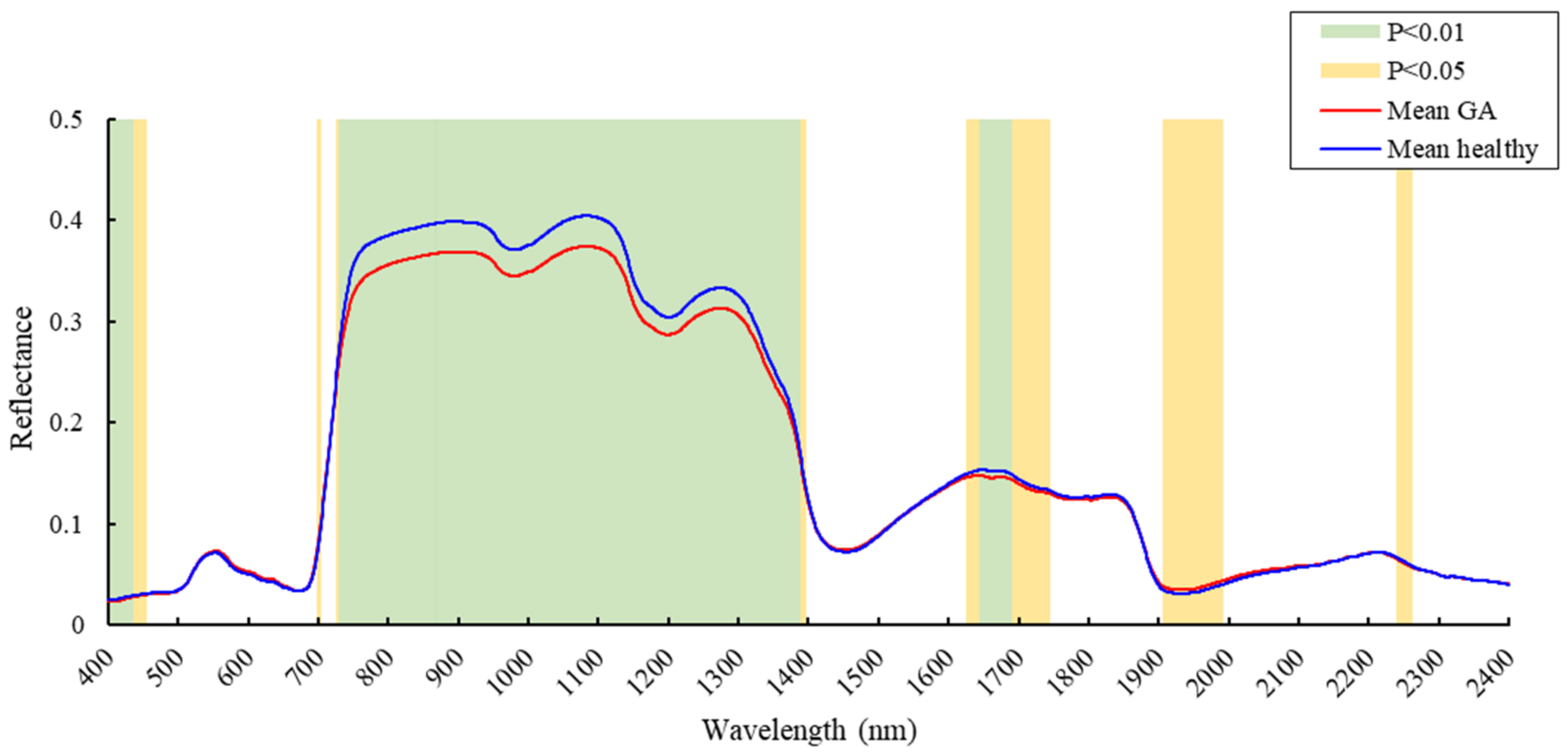
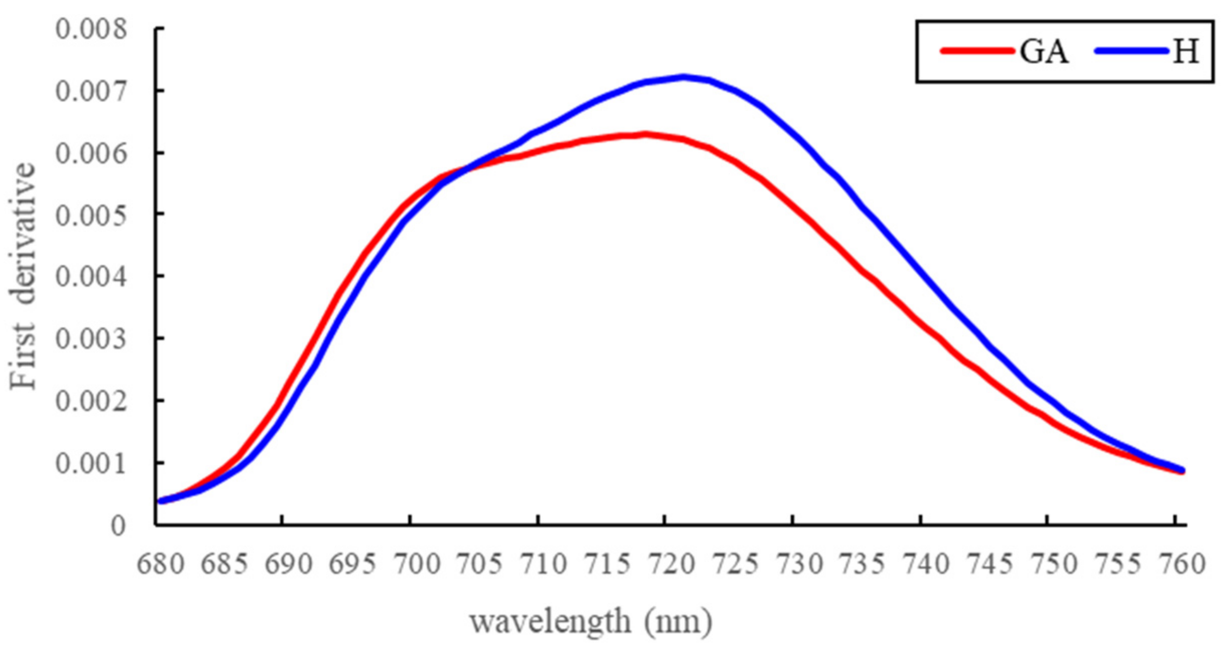
3.1. Spectral Reflectance Analysis

The Mann–Whitney U-test result showed that the spectral reflectance between healthy and GA trees was significantly different (p < 0.05) for 954 wavebands, among which 740 wavebands were highly significant (p < 0.01) (Figure 5). The spectral reflectance of GA trees significantly decreased in the NIR plateau, while the differences were slighter in visible and SWIR regions. Compared with healthy trees, the red-edge position of GA trees shifted toward shorter wavelengths (“blue shift”) and the red-edge slope decreased (Figure 6). In the SWIR region, the features associated with water absorption (near 1450 and 1950 nm) all increased slightly, while only the changes in the second water absorption feature (near 1950 nm) were significant. The mean reflectance of GA trees slightly decreased both in 1625–1743 nm and 2238–2260 nm.

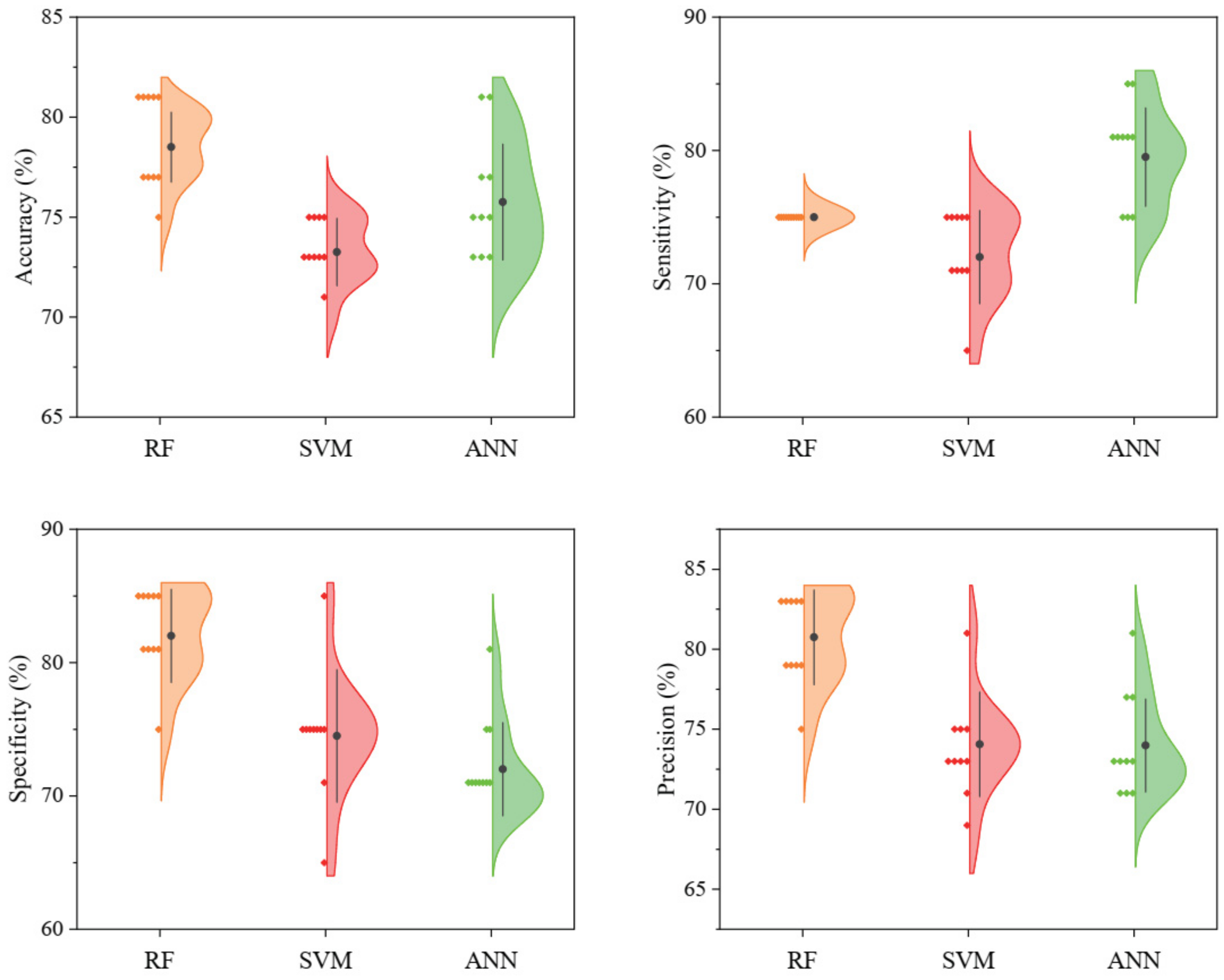
3.2. Classification Models

Three ML algorithms were used to dichotomize the early-infested and healthy trees, and all classification models achieved acceptable accuracy (Figure 7). The RF performed best, with a mean accuracy of 78.50%. The ANN followed with a mean accuracy of 75.75%. The SVM performed the worst, with a mean accuracy of 73.25%. The sensitivity of ANN was significantly higher than RF and SVM (p < 0.01), while the RF had the most stable performance with a sensitivity of 75%. RF had the highest specificity, while there was no significant difference between ANN and SVM. For precision, the RF performed better than ANN and SVM, with a mean precision of 80.75%. The best classification models using three ML algorithms were shown in Table 3. The accuracy of RF and ANN classification models was the same (80%), but the sensitivity of the ANN model was higher than RF.

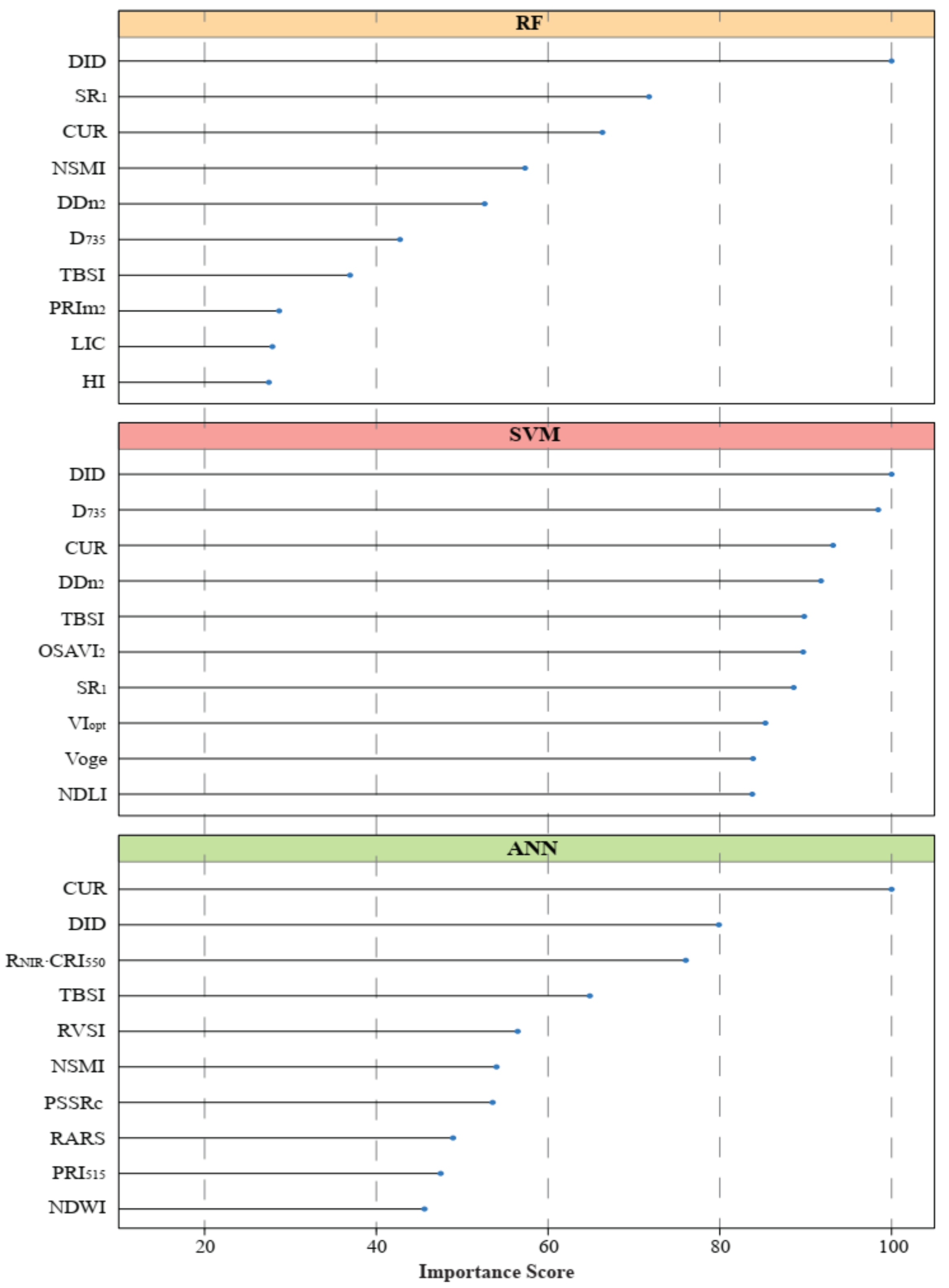
3.3. Important Variables

The variable importance scores for the three best classifiers (Table 3) were ranked, and the top 10 were plotted (Figure 8). The three classification models had different evaluation criteria for the importance of each variable, and different results were obtained. However, some indices had high importance in different models. DID, CUR and TBSI were ranked in the top 10 by all three models. DDn2, SR1 and D735 were important for the RF and SVM models, while NSMI was important for the RF and ANN models. In addition, RNIR•CRI550 and RVSI were important for the ANN model, ranking third and fifth, respectively. The spectral regions covered by these indices include green, red, red-edge, NIR and SWIR.

4. Discussion

Early detection of RTB infestation allows timely action to halt its spread and prevent a pest epidemic. In this study, ground-based hyperspectral data combined with ML algorithms were used to detect pines infested by RTB before obvious discoloration. We determined the spectral regions and important SVIs to differentiate GA pines from the healthy pines.

4.1. Spectral Changes at the GA Stage

Differences in spectral reflectance between GA and healthy classes are shown in Figure 4. Compared with healthy trees, the changes in the visible region (400–760 nm) of infested trees were subtle, which was inconsistent with previous studies [28,35,36,38], in which they found that the reflectance increased significantly, and the green peak (near 550 nm) and red edge (680–760 nm) were important features for detecting stress. These spectral changes were in response to changes in the pigment content of needles, particularly chlorophyll degradation [76]. However, in this study, changes were observed only in red-edge features (position and slope), while the green peak changed indistinctively. This may be due to the slight change of pigment content of pines infested by RTB in this study. Cheng et al. [37] also found that chlorophyll content did not decrease significantly in trees infested by MPB at the GA stage but decreased in grilled trees. Moreover, the blue and red spectra were the strong absorption bands of pigments with high pigment absorption coefficients, which meant that low pigment concentrations could saturate the spectral absorption characteristics and made these regions insensitive to slight pigment changes [28]. Ahern [35] also found that the absorption at 676 nm was still present in yellow needles. Thus, mild pigment changes may not be reflected in the spectrum.
There were evident differences in the NIR and lower SWIR regions (760–1394 nm) between healthy and infested trees in this study. The decreasing trend of reflectance of infested trees in this region was in line with the results of previous studies on other bark beetles [31,38,40]. The high reflectance in this region is the result of leaf scattering, and there are several absorption features associated with water and other chemicals (e.g., starch, protein, lignin and cellulose) [76]. The decrease in reflectance may be due to the changes of leaves’ internal structures, such as cell arrangement or cell–wall/air–space interface [77]. In addition, stomatal closure to preserve water may also result in reduced NIR reflectance [78]. Although the mechanism is unknown, the obvious differences suggested the potential of this region for the early detection of RTB infestation. The potential of the NIR region for the early detection of stress has also been noted in previous studies [8,35,37].
In the SWIR region, the reflectance is mainly related to foliage moisture content, and water absorption features are centered at approximately 1450 and 1950 nm [79]. The reflectance increase from 1906 nm to 1990 nm may be the result of water stress after the RTB attack. Besides moisture, several organic compounds, such as lignin, cellulose, starch, sugar, protein, oil and nitrogen, contribute to the spectral features of the SWIR region. Deformation of the O–H, C–H or N–H bond in these substances results in some minor absorption features in NIR and SWIR regions [76,77]. Differences in spectral reflectance between 1625–1743 nm and 2238–2260 nm could be attributed to changes in concentrations of these substances. Our findings are partially consistent with Abdulah [38]; in his research, there were significant differences in the two SWIR regions (1430–1500 nm and 1897–2000 nm) between healthy and European spruce bark beetle early-infested trees. They explained that this variation was caused by lower water and nitrogen content in green attacked samples.
In general, we found that the reflectance in the NIR region decreased significantly after the RTB attack, and the changes were earlier than those in the visible region, implying the potential of this region for early detection.

4.2. Classification Models and Variable Importance Evaluation

Three ML algorithms, which were widely used in processing remote sensing data, were used to build classification models of early-infested and healthy pines in this study. During model tuning, a random search process was executed to find the best parameters, which did not restrict the parameter range and can traverse all parameter spaces to find the best combination of parameters [44]. To better evaluate the performance of the models, we established ten models using each ML algorithm and conducted one-way ANOVA. Although the average accuracy of RF was the highest, the sensitivity deserves more attention for forest managers because it could represent the missed diagnosis rate of infested pines. Therefore, the ANN performed best with an average sensitivity of 79.5%. However, it should be noted that the same algorithm may perform differently in different studies [9,33,34], and algorithm selection needs to be determined according to a particular situation. In addition, deep learning has been proven to perform well in remote sensing data processing [71], and further research could combine deep learning with hyperspectral data to explore the early detection of RTB infestation.
Numerous studies have established the correlation between SVIs and physiological or biochemical properties of plants and indicated that SVIs can be better indicators of stress [40,80]. SVIs are also applied to reduce the influence of geometry, background and light conditions, which are important for large-scale (e.g., canopy or individual tree) detection [77]. In this study, SVI computations and a feature selection program were executed to transform the high-dimensional spectral reflectance before modeling, which could remove redundant information and simplify the models. The classification results show that SVIs could be used to distinguish early-infested trees from healthy trees.

4.3. Implications for Remote Sensing

Our study identified the spectral changes of P. tabuliformis in the early stage of RTB attack and determined sensitive spectral regions for early detection. These can guide the selection of sensors for large-scale detection. For example, Sentinel-2 has six bands with center wavelengths at 729–1386 nm where the reflectance of infested trees decreased significantly, suggesting its potential for early detection of RTB damage at the stand or landscape scale. Moreover, we screened out several important SVIs for early detection of RTB infestation, and some similar indices might be obtained based on Sentinel-2 bands, such as TBSI, which was a combination of green, red and red-edge bands. Continuous SVI images based on time series of EO data may realize the temporal monitoring of the development dynamics and spread direction of RTB attack [17,81]. The same enlightenment also applies to remote sensing data based on UAVs. However, several points need to be kept in mind when extending these findings to the canopy level. First, the influence of canopy structure parameters on the spectrum may confuse the influence of leaf internal structure, which could lead to uncertain results [25,31]. Second, environmental factors, such as atmospheric moisture, light and understory background, need to be considered when using UAVs or satellites to identify infested individual trees, which may reduce the signal-to-noise ratio [27,28]. Finally, data acquisition time is critical for the early detection of stress using remote sensing [28,78]. On the premise of comprehensive consideration of biological and detection accuracy, remote sensing data acquisition should be more likely to be advanced in order to allow time for subsequent control measures.

5. Conclusions

This is the first study of the spectral changes of P. tabuliformis at the GA stage after RTB attacking. It explored the possibility of early detection of RTB infestation using hyperspectral data. The main conclusions were as follows:
(1) The spectral reflectance of early-infested Chinese pines was significantly different from healthy trees in 954 wavebands between 400 and 2400 nm, and the NIR region was more sensitive to RTB attack than the visible and SWIR regions.
(2) Early-infested trees could be distinguished by SVIs and ML algorithms. The artificial neural network (ANN) classifier performed best with an average sensitivity of 79.5%.
(3) Several SVIs (DID, CUR, TBSI, DDn2, D735, SR1, NSMI, RNIR•CRI550 and RVSI) were important for classification models, indicating their potential for early detection.
In conclusion, this study demonstrated the potential of remote sensing technology for the early detection of RTB infestation. The results provide a reference for larger-scale early detection based on UAV and satellite platforms. Further research is required to examine the changes in the physiological and biochemical properties of needles, which can provide explanations for the spectral changes. The spectral vegetation indices used in this study were proposed by previous studies, and future research can develop more sensitive indices based on spectral and biochemical properties to enhance the operability of remote sensing for the early detection of RTB infestation.

Author Contributions

Conceptualization, Y.L. and L.R.; methodology, B.G. and L.Y.; software, B.G.; validation, B.G.; formal analysis, B.G.; investigation, B.G. and Z.Z.; writing—original draft preparation, B.G.; writing—review and editing, B.G., L.Y. and L.R.; project administration, Y.L.; funding acquisition, Y.L. All authors have read and agreed to the published version of the manuscript.

Funding

This research was funded by the Chinese National Natural Science Foundation (31870642) and Beijing’s Science and Technology Planning Project (Z201100008020001).

Institutional Review Board Statement

Not applicable.

Informed Consent Statement

Not applicable.

Data Availability Statement

Not applicable.

Acknowledgments

The authors would like to thank Heilihe National Natural Reserve and Ningcheng County Heilihe Forest Farm for the field investigation.

Conflicts of Interest

The authors declare no conflict of interest.

References

  1. Yan, Z.; Sun, J.; Don, O.; Zhang, Z. The red turpentine beetle, Dendroctonus valens LeConte (Scolytidae): An exotic invasive pest of pine in China. Biodivers. Conserv. 2005, 14, 1735–1760. [Google Scholar] [CrossRef]
  2. Xu, H.; Li, Y.; Li, Z. The analysis of outbreak reason and spread direction of Dendroctonus valens. Plant Quar. 2006, 20, 278–280. [Google Scholar]
  3. Ge, X.; Jiang, C.; Chen, L.; Qiu, S.; Zhao, Y.; Wang, T.; Zong, S. Predicting the potential distribution in China of Dendroctonus valens Leconte. Environ. Environ. Entomol. 2018, 40, 758–768. [Google Scholar]
  4. Pan, J. Invasive Characteristics, Spatial Distribution and Sampling Technique of Dendroctonus valens Population. Master’s Thesis, Beijing Forestry University, Beijing, China, 2011. [Google Scholar]
  5. Zhang, L.; Chen, Q.; Zhang, X. Studies on the morphological characters and bionomics of Dendroctonus valens Leconte. Sci. Silvae Sin. 2002, 38, 95–99. [Google Scholar]
  6. Zhao, J.; Yang, Z.; Ren, X.; Liang, X. Biological characteristics and occurring law of Dendroctonus valens in China. Sci. Silvae Sin. 2008, 44, 99–105. [Google Scholar]
  7. Wulder, M.A.; Dymond, C.C.; White, J.; Leckie, D.G.; Carroll, A.L. Surveying mountain pine beetle damage of forests: A review of remote sensing opportunities. For. Ecol. Manag. 2006, 221, 27–41. [Google Scholar] [CrossRef]
  8. Foster, A.C.; Walter, J.A.; Shugart, H.H.; Sibold, J.; Negron, J. Spectral evidence of early-stage spruce beetle infestation in Engelmann spruce. For. Ecol. Manag. 2017, 384, 347–357. [Google Scholar] [CrossRef] [Green Version]
  9. Zhan, Z.; Yu, L.; Li, Z.; Ren, L.; Gao, B.; Wang, L.; Luo, Y. Combining GF-2 and Sentinel-2 images to detect tree mortality caused by red turpentine beetle during the early outbreak stage in North China. Forests 2020, 11, 172. [Google Scholar] [CrossRef] [Green Version]
  10. Hall, R.J.; Castilla, G.; White, J.C.; Cooke, B.J.; Skakun, R.S. Remote sensing of forest pest damage: A review and lessons learned from a Canadian perspective. Can. Entomol. 2016, 148, S296–S356. [Google Scholar] [CrossRef]
  11. Lausch, A.; Erasmi, S.; King, D.J.; Magdon, P.; Heurich, M. Understanding forest health with remote sensing-Part I—A review of spectral traits, processes and remote-sensing characteristics. Remote Sens. (Basel) 2016, 8, 1029. [Google Scholar] [CrossRef] [Green Version]
  12. Lausch, A.; Erasmi, S.; King, D.J.; Magdon, P.; Heurich, M. Understanding forest health with remote sensing-Part II—A review of approaches and data models. Remote Sens. 2017, 9, 129. [Google Scholar] [CrossRef] [Green Version]
  13. Stone, C.; Mohammed, C. Application of remote sensing technologies for assessing planted forests damaged by insect pests and fungal pathogens: A review. Curr. For. Rep. 2017, 3, 75–92. [Google Scholar] [CrossRef]
  14. Senf, C.; Seidl, R.; Hostert, P. Remote sensing of forest insect disturbances: Current state and future directions. Int. J. Appl. Earth Obs. Geoinf. 2017, 60, 49–60. [Google Scholar] [CrossRef] [Green Version]
  15. Goodwin, N.R.; Coops, N.C.; Wulder, M.A.; Gillanders, S.; Schroeder, T.A.; Nelson, T. Estimation of insect infestation dynamics using a temporal sequence of Landsat data. Remote Sens. Environ. 2008, 112, 3680–3689. [Google Scholar] [CrossRef]
  16. Liang, L.; Chen, Y.; Hawbaker, T.J.; Zhu, Z.; Gong, P. Mapping mountain pine beetle mortality through growth trend analysis of time-series Landsat data. Remote Sens. 2014, 6, 5696–5716. [Google Scholar] [CrossRef] [Green Version]
  17. Grabska, E.; Hawryło, P.; Socha, J. Continuous detection of small-scale changes in scots pine dominated stands using dense Sentinel-2 time series. Remote Sens. 2020, 12, 1298. [Google Scholar] [CrossRef] [Green Version]
  18. Gomez, D.; Ritger, H.; Pearce, C.; Eickwort, J.; Hulcr, J. Ability of remote sensing systems to detect bark beetle spots in the southeastern US. Forests 2020, 11, 1167. [Google Scholar] [CrossRef]
  19. Meddens, A.J.H.; Hicke, J.A.; Vierling, L.A.; Hudak, A.T. Evaluating methods to detect bark beetle-caused tree mortality using single-date and multi-date Landsat imagery. Remote Sens. Environ. 2013, 132, 49–58. [Google Scholar] [CrossRef]
  20. Abdullah, H.; Skidmore, A.K.; Darvishzadeh, R.; Heurich, M. Sentinel-2 accurately maps green-attack stage of European spruce bark beetle (Ips typographus, L.) compared with Landsat-8. Remote Sens. Ecol. Conserv. 2018, 5, 87–106. [Google Scholar] [CrossRef] [Green Version]
  21. Abdullah, H.; Darvishzadeh, R.; Skidmore, A.K.; Heurich, M. Sensitivity of Landsat-8 OLI and TIRS data to foliar properties of early stage bark beetle (Ips typographus, L.) infestation. Remote Sens. 2019, 11, 398. [Google Scholar] [CrossRef] [Green Version]
  22. Huo, L.; Persson, H.J.; Lindberg, E. Early detection of forest stress from European spruce bark beetle attack, and a new vegetation index: Normalized distance red & SWIR (NDRS). Remote Sens. Environ. 2021, 255, 112240. [Google Scholar] [CrossRef]
  23. Bárta, V.; Lukeš, P.; Homolová, L. Early detection of bark beetle infestation in Norway spruce forests of Central Europe using Sentinel-2. Int. J. Appl. Earth Obs. Geoinf. 2021, 100, 102335. [Google Scholar] [CrossRef]
  24. White, J.C.; Wulder, M.; Brooks, D.; Reich, R. Detection of red attack stage mountain pine beetle infestation with high spatial resolution satellite imagery. Remote Sens. Environ. 2005, 96, 340–351. [Google Scholar] [CrossRef]
  25. Coops, N.C.; Johnson, M.; Wulder, M.; White, J. Assessment of QuickBird high spatial resolution imagery to detect red attack damage due to mountain pine beetle infestation. Remote Sens. Environ. 2006, 103, 67–80. [Google Scholar] [CrossRef]
  26. Dennison, P.E.; Brunelle, A.R.; Carter, V.A. Assessing canopy mortality during a mountain pine beetle outbreak using GeoEye-1 high spatial resolution satellite data. Remote Sens. Environ. 2010, 114, 2431–2435. [Google Scholar] [CrossRef]
  27. Immitzer, M.; Atzberger, C. Early detection of bark beetle infestation in Norway Spruce (Picea abies L.) using WorldView-2 data. Photogramm. Fernerkund. Geoinf. 2014, 5, 351–367. [Google Scholar] [CrossRef]
  28. Mullen, K. Early Detection of Mountain Pine Beetle Damage in Ponderosa Pine Forests of the Black Hills Using Hyperspectral and WorldView-2 Data. Master’s Thesis, Minnesota State University, Mankato, MN, USA, 2016. [Google Scholar]
  29. Lausch, A.; Heurich, M.; Gordalla, D.; Dobner, H.-J.; Gwillym-Margianto, S.; Salbach, C. Forecasting potential bark beetle outbreaks based on spruce forest vitality using hyperspectral remote-sensing techniques at different scales. For. Ecol. Manag. 2013, 308, 76–89. [Google Scholar] [CrossRef]
  30. Fassnacht, F.E.; Latifi, H.; Ghosh, A.; Joshi, P.K.; Koch, B. Assessing the potential of hyperspectral imagery to map bark beetle-induced tree mortality. Remote Sens. Environ. 2014, 140, 533–548. [Google Scholar] [CrossRef]
  31. Niemann, K.O.; Quinn, G.; Stephen, R.; Visintini, F.; Parton, D. Hyperspectral remote sensing of mountain pine beetle with an emphasis on previsual assessment. Can. J. Remote Sens. 2015, 41, 191–202. [Google Scholar] [CrossRef]
  32. Näsi, R.; Honkavaara, E.; Lyytikäinen-Saarenmaa, P.; Blomqvist, M.; Litkey, P.; Hakala, T.; Viljanen, N.; Kantola, T.; Tanhuanpää, T.; Holopainen, M. Using UAV-based photogrammetry and hyperspectral imaging for mapping bark beetle damage at tree-level. Remote Sens. 2015, 7, 15467–15493. [Google Scholar] [CrossRef] [Green Version]
  33. Näsi, R.; Honkavaara, E.; Blomqvist, M.; Lyytikäinen-Saarenmaa, P.; Hakala, T.; Viljanen, N.; Kantola, T.; Holopainen, M. Remote sensing of bark beetle damage in urban forests at individual tree level using a novel hyperspectral camera from UAV and aircraft. Urban For. Urban Green. 2018, 30, 72–83. [Google Scholar] [CrossRef]
  34. Honkavaara, E.; Näsi, R.; Oliveira, R.; Viljanen, N.; Suomalainen, J.; Khoramshahi, E.; Hakala, T.; Nevalainen, O.; Markelin, L.; Vuorinen, M.; et al. Using multitemporal hyper- and multispectral Uav imaging for detecting bark beetle infestation on Norway spruce. Int. Arch. Photogramm. Remote Sens. Spat. Inf. Sci. 2020, XLIII-B3-2, 429–434. [Google Scholar] [CrossRef]
  35. Ahern, F.J. The effects of bark beetle stress on the foliar spectral reflectance of lodgepole pine. Int. J. Remote Sens. 1988, 9, 1451–1468. [Google Scholar] [CrossRef]
  36. Reichmuth, A.; Henning, L.; Pinnel, N.; Bachmann, M.; Rogge, D. Early detection of vitality changes of multi-temporal Norway spruce laboratory needle measurements—The ring-barking experiment. Remote Sens. 2018, 10, 57. [Google Scholar] [CrossRef] [Green Version]
  37. Cheng, T.; Rivard, B.; Sanchez-Azofeifa, A.; Feng, J.; Calvo-Polanco, M. Continuous wavelet analysis for the detection of green attack damage due to mountain pine beetle infestation. Remote Sens. Environ. 2010, 114, 899–910. [Google Scholar] [CrossRef]
  38. Abdullah, H.; Darvishzadeh, R.; Skidmore, A.K.; Groen, T.A.; Heurich, M. European spruce bark beetle (Ips typographus, L.) green attack affects foliar reflectance and biochemical properties. Int. J. Appl. Earth Obs. Geoinf. 2018, 64, 199–209. [Google Scholar] [CrossRef] [Green Version]
  39. Ismail, R.; Mutanga, O. Discriminating the early stages of Sirex noctilio infestation using classification tree ensembles and shortwave infrared bands. Int. J. Remote Sens. 2011, 32, 4249–4266. [Google Scholar] [CrossRef]
  40. Liu, Y.; Zhan, Z.; Ren, L.; Ze, S.; Yu, L.; Jiang, Q.; Luo, Y. Hyperspectral evidence of early-stage pine shoot beetle attack in Yunnan pine. For. Ecol. Manag. 2021, 497, 119505. [Google Scholar] [CrossRef]
  41. Yu, R.; Ren, L.; Luo, Y. Early detection of pine wilt disease in Pinus tabuliformis in North China using a field portable spectrometer and UAV-based hyperspectral imagery. For. Ecosyst. 2021, 8, 44. [Google Scholar] [CrossRef]
  42. Liu, Y. A comparative study on feature selection methods for drug discovery. J. Chem. Inf. Comput. Sci. 2004, 44, 1823–1828. [Google Scholar] [CrossRef] [Green Version]
  43. Kushmerick, N. Wrapper induction: Efficiency and expressiveness. Artif. Intell. 2000, 118, 15–68. [Google Scholar] [CrossRef] [Green Version]
  44. Burger, S.V. Introduction to Machine Learning with R; O’Reilly Media, Inc.: Sebastopol, CA, USA, 2018. [Google Scholar]
  45. Beck, P.; Zarco-Tejada, P.J.; Strobl, P.; San Miguel, J. The Feasibility of Detecting Trees Affected by the Pine Wood Nematode Using Remote Sensing; Publications Office of the European Union: Luxembourg, 2015; pp. 1831–9424. [Google Scholar]
  46. Tian, Y.-C.; Gu, K.-J.; Chu, X.; Yao, X.; Cao, W.-X.; Zhu, Y. Comparison of different hyperspectral vegetation indices for canopy leaf nitrogen concentration estimation in rice. Plant Soil 2013, 376, 193–209. [Google Scholar] [CrossRef]
  47. Carter, G.A.; Miller, R.L. Early detection of plant stress by digital imaging within narrow stress-sensitive wavebands. Remote Sens. Environ. 1994, 50, 295–302. [Google Scholar] [CrossRef]
  48. Zhu, Y.; Yao, X.; Tian, Y.; Liu, X.; Cao, W. Analysis of common canopy vegetation indices for indicating leaf nitrogen accumulations in wheat and rice. Int. J. Appl. Earth Obs. Geoinf. 2008, 10, 1–10. [Google Scholar] [CrossRef]
  49. Blackburn, G.A. Spectral indices for estimating photosynthetic pigment concentrations: A test using senescent tree leaves. Int. J. Remote Sens. 1998, 19, 657–675. [Google Scholar] [CrossRef]
  50. Chappelle, E.W.; Kim, M.S.; McMurtrey, J.E., III. Ratio analysis of reflectance spectra (RARS): An algorithm for the remote estimation of the concentrations of chlorophyll a, chlorophyll b, and carotenoids in soybean leaves. Remote Sens. Environ. 1992, 39, 239–247. [Google Scholar] [CrossRef]
  51. Ceccato, P.; Flasse, S.; Tarantola, S.; Jacquemoud, S.; Grégoire, J.-M. Detecting vegetation leaf water content using reflectance in the optical domain. Remote Sens. Environ. 2001, 77, 22–33. [Google Scholar] [CrossRef]
  52. Lichtenthaler, H.K.; Lang, M.; Sowinska, M.; Heisel, F.; Miehé, J.A. Detection of vegetation stress via a new high resolution fluorescence imaging system. J. Plant Physiol. 1996, 148, 599–612. [Google Scholar] [CrossRef]
  53. Lee, Y.-J.; Yang, C.-M.; Chang, K.-W.; Shen, Y. A simple spectral index using reflectance of 735 nm to assess nitrogen status of rice canopy. Agron. J. 2008, 100, 205–212. [Google Scholar] [CrossRef]
  54. Vogelmann, J.E.; Rock, B.N.; Moss, D.M. Red edge spectral measurements from sugar maple leaves. Int. J. Remote Sens. 1993, 14, 1563–1575. [Google Scholar] [CrossRef]
  55. Gamon, J.A.; Peñuelas, J.; Field, C.B. A narrow-waveband spectral index that tracks diurnal changes in photosynthetic efficiency. Remote Sens. Environ. 1992, 41, 35–44. [Google Scholar] [CrossRef]
  56. Merton, R.; Huntington, J. Early simulation results of the ARIES-1 satellite sensor for multi-temporal vegetation research derived from AVIRIS. In Proceedings of the Eighth Annual JPL Airborne Earth Science Workshop, Pasadena, CA, USA, 9–11 February 1999. [Google Scholar]
  57. Gitelson, A.A.; Zur, Y.; Chivkunova, O.B.; Merzlyak, M.N. Assessing carotenoid content in plant leaves with reflectance spectroscopy. Photochem. Photobiol. 2002, 75, 272–281. [Google Scholar] [CrossRef]
  58. Gitelson, A.A.; Gritz, Y.; Merzlyak, M.N. Relationships between leaf chlorophyll content and spectral reflectance and algorithms for non-destructive chlorophyll assessment in higher plant leaves. J. Plant Physiol. 2003, 160, 271–282. [Google Scholar] [CrossRef] [PubMed]
  59. Gitelson, A.A.; Viña, A.; Ciganda, V.; Rundquist, D.C.; Arkebauer, T.J. Remote estimation of canopy chlorophyll content in crops. Geophys. Res. Lett. 2005, 32, L08403. [Google Scholar] [CrossRef] [Green Version]
  60. Zarco-Tejada, P.J.; Miller, J.R.; Noland, T.L.; Mohammed, G.H.; Sampson, P.H. Scaling-up and model inversion methods with narrowband optical indices for chlorophyll content estimation in closed forest canopies with hyperspectral data. IEEE Trans. Geosci. Remote Sens. 2001, 39, 1491–1507. [Google Scholar] [CrossRef] [Green Version]
  61. Gao, B.-C. NDWI—A normalized difference water index for remote sensing of vegetation liquid water from space. Remote Sens. Environ. 1996, 58, 257–266. [Google Scholar] [CrossRef]
  62. Haubrock, S.-N.; Chabrillat, S.; Lemmnitz, C.; Kaufmann, H. Surface soil moisture quantification models from reflectance data under field conditions. Int. J. Remote Sens. 2008, 29, 3–29. [Google Scholar] [CrossRef]
  63. Serrano, L.; Peñuelas, J.; Ustin, S.L. Remote sensing of nitrogen and lignin in Mediterranean vegetation from AVIRIS data: Decomposing biochemical from structural signals. Remote Sens. Environ. 2002, 81, 355–364. [Google Scholar] [CrossRef]
  64. Wang, Q.; Li, P. Hyperspectral indices for estimating leaf biochemical properties in temperate deciduous forests: Comparison of simulated and measured reflectance data sets. Ecol. Indic. 2012, 14, 56–65. [Google Scholar] [CrossRef]
  65. Dash, J.; Curran, P.J. The MERIS terrestrial chlorophyll index. Int. J. Remote Sens. 2004, 25, 5403–5413. [Google Scholar] [CrossRef]
  66. Reyniers, M.; Walvoort, D.J.J.; De Baardemaaker, J. A linear model to predict with a multi-spectral radiometer the amount of nitrogen in winter wheat. Int. J. Remote Sens. 2006, 27, 4159–4179. [Google Scholar] [CrossRef]
  67. Haboudane, D.; Miller, J.R.; Pattey, E.; Zarco-Tejada, P.J.; Strachan, I.B. Hyperspectral vegetation indices and novel algorithms for predicting green LAI of crop canopies: Modeling and validation in the context of precision agriculture. Remote Sens. Environ. 2004, 90, 337–352. [Google Scholar] [CrossRef]
  68. Gao, J.; Liang, T.; Yin, J.; Ge, J.; Feng, Q.; Wu, C.; Hou, M.; Liu, J.; Xie, H. Estimation of alpine grassland forage nitrogen coupled with hyperspectral characteristics during different growth periods on the tibetan plateau. Remote Sens. 2019, 11, 2085. [Google Scholar] [CrossRef] [Green Version]
  69. Wu, C.; Niu, Z.; Tang, Q.; Huang, W. Estimating chlorophyll content from hyperspectral vegetation indices: Modeling and validation. Agric. For. Meteorol. 2008, 148, 1230–1241. [Google Scholar] [CrossRef]
  70. Zhu, X. Playing with R: Data Analitical Thinking to Practice; China Renmin University Press: Beijing, China, 2018. [Google Scholar]
  71. Sothe, C.; De Almeida, C.M.; Schimalski, M.B.; La Rosa, L.E.C.; Castro, J.D.B.; Feitosa, R.Q.; Dalponte, M.; Lima, C.L.; Liesenberg, V.; Miyoshi, G.T.; et al. Comparative performance of convolutional neural network, weighted and conventional support vector machine and random forest for classifying tree species using hyperspectral and photogrammetric data. GISci. Remote Sens. 2020, 57, 369–394. [Google Scholar] [CrossRef]
  72. Gutierrez, D.D. Machine Learning and Data Science: An Introduction to Statistical Learning Methods with R; Technics Publications: Bernards, NJ, USA, 2015. [Google Scholar]
  73. Lesmeister, C. Mastering Machine Learning with R, 2nd ed.; Packt Publishing Ltd: Birmingham, UK, 2017. [Google Scholar]
  74. Rumpf, T.; Mahlein, A.-K.; Steiner, U.; Oerke, E.-C.; Dehne, H.-W.; Plümer, L. Early detection and classification of plant diseases with Support Vector Machines based on hyperspectral reflectance. Comput. Electron. Agric. 2010, 74, 91–99. [Google Scholar] [CrossRef]
  75. Variable Importance. Available online: https://topepo.github.io/caret/variable-importance.html (accessed on 10 March 2021).
  76. Curran, P.J. Remote sensing of foliar chemistry. Remote Sens. Environ. 1989, 30, 271–278. [Google Scholar] [CrossRef]
  77. Runesson, U.T. Considerations for Early Remote Detection of Mountain Pine Beetle in Green-Foliaged Lodgepole Pine. Ph.D. Thesis, University of British Columbia, Vancouver, BC, Canada, 1991. [Google Scholar]
  78. Abdullah, H.; Skidmore, A.K.; Darvishzadeh, R.; Heurich, M. Timing of red-edge and shortwave infrared reflectance critical for early stress detection induced by bark beetle (Ips typographus, L.) attack. Int. J. Appl. Earth Obs. Geoinf. 2019, 82, 101900. [Google Scholar] [CrossRef]
  79. Sims, D.A.; Gamon, J.A. Estimation of vegetation water content and photosynthetic tissue area from spectral reflectance: A comparison of indices based on liquid water and chlorophyll absorption features. Remote Sens. Environ. 2003, 84, 526–537. [Google Scholar] [CrossRef]
  80. Yu, L.; Zhan, Z.; Ren, L.; Zong, S.; Luo, Y.; Huang, H. Evaluating the potential of WorldView-3 data to classify different shoot damage ratios of pinus yunnanensis. Forests 2020, 11, 417. [Google Scholar] [CrossRef] [Green Version]
  81. Yu, L.; Huang, J.; Zong, S.; Huang, H.; Luo, Y. Detecting shoot beetle damage on Yunnan pine using Landsat time-series data. Forests 2018, 9, 39. [Google Scholar] [CrossRef] [Green Version]
Figure 1. Diagram of RTB attack stages.
Remotesensing 14 01373 g001
Figure 2. Sampling locations in Heilihe National Natural Reserve.
Remotesensing 14 01373 g002
Figure 3. A Chinese pine at GA stage. The crown was green (left), and multiple pitch tubes were on the stem (right).
Remotesensing 14 01373 g003
Figure 4. Spectral data acquisition setup.
Remotesensing 14 01373 g004
Figure 5. Mean reflectance of GA stage and healthy trees. The color areas indicate significant differences in the reflectance of wavebands.
Remotesensing 14 01373 g005
Figure 6. First derivative of mean reflectance in red-edge region (680–760 nm).
Remotesensing 14 01373 g006
Figure 7. Performance of the classification models based on SVIs. The black dots represent the mean, and the black lines represent the mean ± SD.
Remotesensing 14 01373 g007
Figure 8. Importance of spectral variables in three classification models.
Remotesensing 14 01373 g008
Table 1. Selection of SVIs as input variables of classifiers.
Spectral IndicesFormulation or DepictionSpectral RegionsRef.
Blue indexBI = R450/R490Blue[45]
Simple ratio indicesSR1 = R545/R538Green[46]
SR2 = R694/R760Red edge[47]
Ratio vegetation indexRVI = R810/R660Red, NIR[48]
Difference vegetation indexDVI = R810 − R680Red edge, NIR[48]
Pigment-specific simple ratioPSSRb= R800/R635Red, NIR[49]
PSSRc = R800/R470Blue, NIR[49]
Pigment-specific normalized differencePSNDa = (R800 − R680)/(R800 + R680)Red edge, NIR[49]
PSNDb = (R800 − R635)/(R800 + R635)Red, NIR[49]
PSNDc = (R800 − R470)/(R800 + R470)Blue, NIR[49]
Ratio analysis of reflectance spectraRARS = R746/R513Green, red edge[50]
Moisture stress indexMSI = R1600/R820NIR, SWIR[51]
Lichtenthaler indexLIC = R440/R740Blue, red edge[52]
First derivative of reflectance spectrum at 735 nmD735Red edge[53]
A ratio of first-derivative valuesVoge = D715/D705Red edge[54]
First-derivative difference indexDID = D1183 − D876NIR[46]
Physiological reflectance indexPRI515 = (R515 − R531)/(R515 + R531)Green[55]
Photochemical reflectance indexPRIm2 = (R600 − R531)/(R600 + R531)Green, orange[45]
PRIm4 = (R570 − R531 − R670)/((R570 + R531 + R670)Green, red[45]
PRIn = PRI570/[RDVI × (R700/R670)],PRI570 = (R570 − R531)/(R570 + R531), RDVI = (R800 − R670)/(R800 + R670)0.5Green, red, NIR[45]
Red-edge vegetation stress indexRVSI = (R714 − R752)/2 − R733Red edge[56]
Carotenoid reflectance indexCRI550 = 1/R510 − 1/R550Green[57]
RNIR•CRI550R770 × CRI550Green, NIR[58]
Chlorophyll content indexCIred-edge = R840~870/R720~730 − 1Red edge, NIR[59]
Curvature indexCUR = R675 × R690/R6832Red, red edge[60]
Normalized difference vegetation indexNDVIg-b = (R537 − R440)/(R537 + R440)Blue, green[46]
Normalized difference water indexNDWI = (R860 − R1240)/(R860 + R1240)NIR[61]
Normalized soil moisture indexNSMI = (R1800 − R2119)/(R1800 + R2119)SWIR[62]
Normalized difference lignin indexNDLI = [log(1/R1754) − log(1/R1680)]/[log(1/R1754) + log(1/R1680)]SWIR[63]
Health indexHI = (R534 − R698)/(R534 + R698) − R704/2Green, red edge[45]
Double-difference indicesDDn1 = 2R715 − R715−185 − R715+185Red, red edge, NIR[64]
DDn2 = 2R1530 − R1530−525 − R1530+525NIR, SWIR[64]
DDn3 = 2R1235 − R1235−25 − R1235+25NIR[64]
MERIS terrestrial chlorophyll indexMTCI = (R754 − R709)/(R709 − R681)Red edge[65]
Optimal vegetation indexVIopt = 1.45 × (R8002 + 1)/(R670 + 0.45)Red, NIR[66]
Three-band spectral indexTBSI = (R605 − R521 − R682)/(R605 + R521 + R682)Green, red, red edge[46]
Modified triangular vegetation indexMTVI = 1.2 × [1.2 × (R800 − R550) − 2.5 × (R670 − R550)]Green, red, NIR[67]
Soil-adjusted vegetation indexSAVI = (1 + 0.5) × [(R800 − R670)/(R800 + R670 + 0.5)]Red, NIR[68]
Optimized SAVIOSAVI1 = (1 + 0.16) × [(R800 − R670)/(R800 + R670 + 0.16)]Red, NIR[69]
OSAVI2 = (1 + 0.16) × [(R750 − R705)/(R750 + R705 + 0.16)]Red edge[69]
Table 2. The calculation formula of four metrics.
True Conditions
Positive (GA)Negative (H)
Test resultsPositive (GA)True positive (TP)False positive (FP)Precision = TP/(TP + FP)
Negative (H)False negative (FN)True negative (TN)
Sensitivity =
TP/(TP + FN)
Specificity =
TN/(FP + TN)
Accuracy =
(TP + TN)/(TP + FP + TN + FN)
Table 3. Hyperparameters and performance of the best classification models using three ML algorithms.
Classification ModelsHyperparametersEvaluation Metrics (%)
Accuracy (Kappa)SensitivitySpecificityPrecision
RFmtry2980 (0.6)758583.33
SVMC21.0838175 (0.5)757575
γ0.010476
ANNsize2080 (0.6)808080
decay0.391524
Publisher’s Note: MDPI stays neutral with regard to jurisdictional claims in published maps and institutional affiliations.

