Smartphone–Camera–Based Water Reflectance Measurement and Typical Water Quality Parameter Inversion

Abstract

Crowdsourced data from smart devices play an increasingly important role in water quality monitoring. However, guaranteeing and evaluating crowdsourced data quality is a key issue. This study aims to extract more accurate water reflectance data from smartphone photographs with variable exposure parameters, and to test the usability of these data in deriving water quality parameters. A set of low–cost reference cards was designed to be placed in the center of the photograph near the water surface, and a calculation model was proposed to convert the photograph digital numbers (DNs) to water reflectance. A nonlinear DN–to–reflectance model was constructed using the inherent reflectance and DN of the reference card in the photograph. Then, the reflectance of the water surface in the same photograph was estimated. During the evaluation of this scheme in seven different waterbodies with 112 sampling sites, small differences were observed between the estimated and measured remote sensing reflectance; the average unbiased relative errors (AUREs) for the red, green, and blue bands were 25.7%, 29.5%, and 35.2%, respectively, while the RMSEs for the three bands were 0.0032, 0.0051, 0.0031, respectively. The derived water reflectance data were used to retrieve the Secchi–disk depth (Z_sd) and turbidity, with accuracies of 72.4% and 60.2%, respectively. The results demonstrate that the proposed method based on the smartphone camera can be used to derive the remote sensing reflectance and water quality parameters effectively with acceptable accuracy.

1. Introduction

To slow and reverse the deterioration of water quality, it is necessary to strengthen the monitoring, evaluation, and governance of surface water quality. Traditional water quality monitoring mainly relies on collecting water samples on site and sending them to the laboratory to measure various water quality parameters. This method has the advantage that many different water quality parameters can be measured, with relatively high accuracy. However, the disadvantage is that water quality data can only be collected at limited time points, and the sampling interval is usually long. This is because such sampling usually requires professional equipment and trained technicians, and many of the instruments are expensive, heavy, inconvenient to carry, and labor intensive. The development of satellite remote sensing technology provides a feasible way to monitor water quality across large areas and long time series, and to further discover the temporal and spatial distribution characteristics and migration paths of pollutants [1]. However, its application is strongly affected by the satellite revisit period, remote sensing data resolution, and cloud coverage, among other factors. With the rapid development of modern big data technology and communication technology, as well as increasing public interest in environmental quality, water quality monitoring is no longer limited to traditional observational and remote sensing data; environmental monitoring has gradually entered the era of multi–source big data [2,3,4,5]. In this regard, intelligent mobile devices show great potential, providing new possibilities for water quality monitoring.

Digital cameras and smartphone cameras have high spatial resolution and time flexibility and are not affected by cloud coverage. Thus, they can complement satellite remote sensing technology, which is affected by cloud coverage. However, how to make effective quantitative use of the citizen science data acquired from the handheld cameras and incorporate it into scientific research is a difficult issue to tackle. Sequoia Scientific Inc. has developed the HydroColor mobile application available at http://misclab.umeoce.maine.edu/research/HydroColor.php (accessed on 7 March 2022), which uses a mobile phone camera as a three–band remote sensing spectral radiometer. The user takes a series of three–band pictures according to the guiding information, calculates the red, green, and blue wide bands of the water–leaving reflectance from these pictures, and estimates the water turbidity and suspended matter on this basis [6,7]. Because the reference card must be photographed, HydroColor is not friendly to non–professional users. Moreover, the water–leaving reflectance calculation can be seriously affected by the bidirectionality of the reference card. HydroColor also faces some technical problems, such as a lack of correction for changes in camera exposure parameters and the nonlinear response of DNs, resulting in large uncertainties in the inversion results [8,9,10,11]. As stated above, there are various problems related to the quantitative application of water surface photographs. There is an urgent need to develop a stable and applicable method to retrieve more accurate water reflectance and water quality data based on smartphone photographs.

A digital camera can be seen as a multispectral remote sensor with three visible bands: red, green, and blue. Many multispectral satellites, such as the Landsat TM and ETM+ imagery and MODIS land surface reflectance products, also include only three visible bands, and these bands have been applied for the inversion of typical water quality parameters. Liu et al. [12] constructed a transparency inversion model of green and red band means based on MODIS and used it to analyze the temporal and spatial variation law of transparency of large lakes in China from 2000 to 2018. Lathrop and Lillesand [13] used the SPOT–1 green wave band to estimate water transparency in Green Bay and Lake Michigan in the United States. Binding et al. [14] used the good relationship between the green band near 550 nm and the transparency to monitor the water transparency of the Great Lakes of North America from 1979 to 1985 and from 1998 to 2006 with the data from the Coastal Zone Color Scanner and the Sea–viewing Wide Field–of–view Sensor. Olmanson et al. [15] established a water transparency model using the blue:red band ratio of Landsat data, and applied it to retrieve the water transparency and the trophic state of Minnesota lakes from 1985 to 2005. They then analyzed the distribution and changes in the water transparency and trophic state of these lakes over the 20 years. Song et al. [16] used the normalized value model of red and green light for the turbidity inversion of Taihu Lake from Landsat8 OLI images. In addition to the above band combination methods, the visible red, green, and blue bands have also been used to obtain the Forel–Ule index, and then to retrieve the water quality of waterbodies. Wang et al. [17] developed a Forel–Ule index calculation method based on MODIS red, green, and blue bands, and further applied it to transparency estimation [18] and trophic state index evaluation [19]. These studies show that remote sensing data comprising three visible bands can be used for the inversion of typical water quality parameters, which has supported the inversion of water quality parameters using water surface photographs with only three visible bands.

Citizen science plays an increasingly important role in water quality monitoring and can be used as a complementary means to the remote sensing of water quality. The smartphone camera is a convenient and useful tool in obtaining crowdsourced data in citizen science. However, a key issue to tackle is to control the quality of crowdsourced data and make quantification use of these data so that they can be smoothly combined with remote sensing data. In this study, we develop a low–cost reference card–assisted scheme to derive water reflectance data with a smartphone camera. This scheme was further evaluated through the derivation of remote sensing reflectance (R_rs, sr⁻¹) and water quality parameters in seven water bodies.

2. Study Area and Datasets

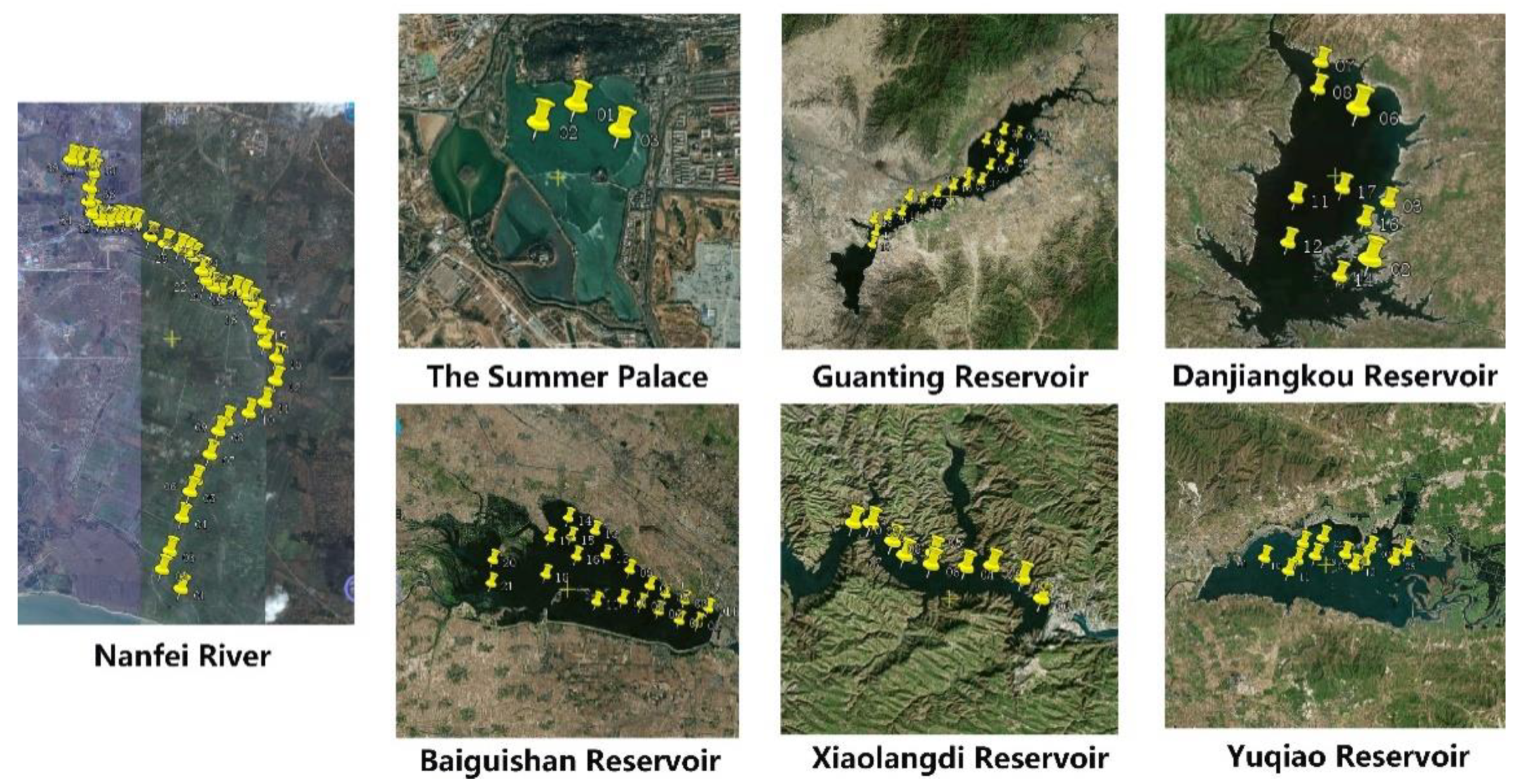
2.1. Study Area

In 2020, we carried out a series of field measurement experiments in seven study areas, including the Nanfei River, the Summer Palace, Guanting Reservoir, Danjiangkou Reservior, Baiguishan Reservior, Xiaolangdi Reservior and Yuqiao Reservior (Figure 1). The locations, sampling times, and number of sampling sites are shown in

Table 1. Overview of the water quality monitoring experiment, based on automatic exposure of smartphones.

Research Area Name	Center Longitude	Center Latitude	Sampling Date	Time Range (Local Time)	Sampling Number
Nanfei River	117.40E	31.77N	22 May 2020	9:30–15:45	40
The SummerPalace	116.27E	39.99N	19 June 2020	10:15–14:15	3
Guanting Reservoir	115.73E	40.34N	13 August 2020	9:55–13:50	18
Danjiangkou Reservoir	110.58E	32.74N	2 September 2020	9:30–15:45	9
Baiguishan Reservoir	113.19E	33.73N	4 September 2020	10:15–14:15	20
Xiaolangdi Reservoir	112.33E	34.94N	22 October 2020	9:55–13:50	10
Yuqiao Reservoir	117.53E	40.04N	8 November 2020	9:30–15:45	12

. During the experiments, the weather was sunny, without any clouds near the sun. The experiments were carried out at 9:30–15:45 local time, and the solar zenith angles ranged from 16° to 66°.

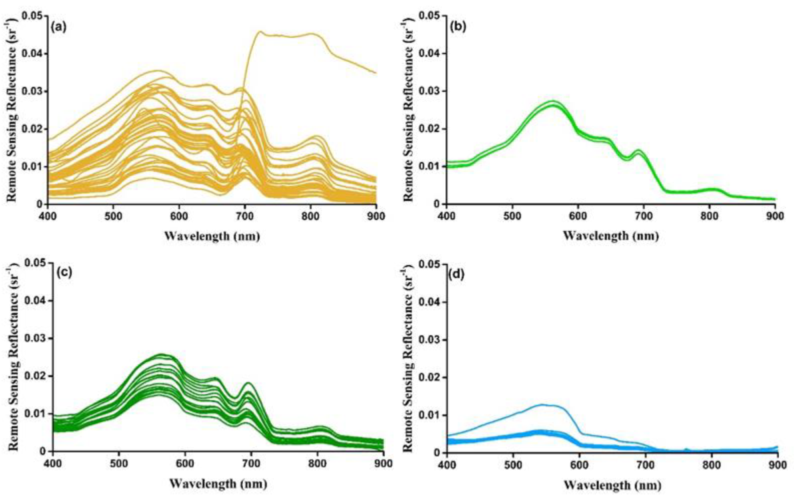
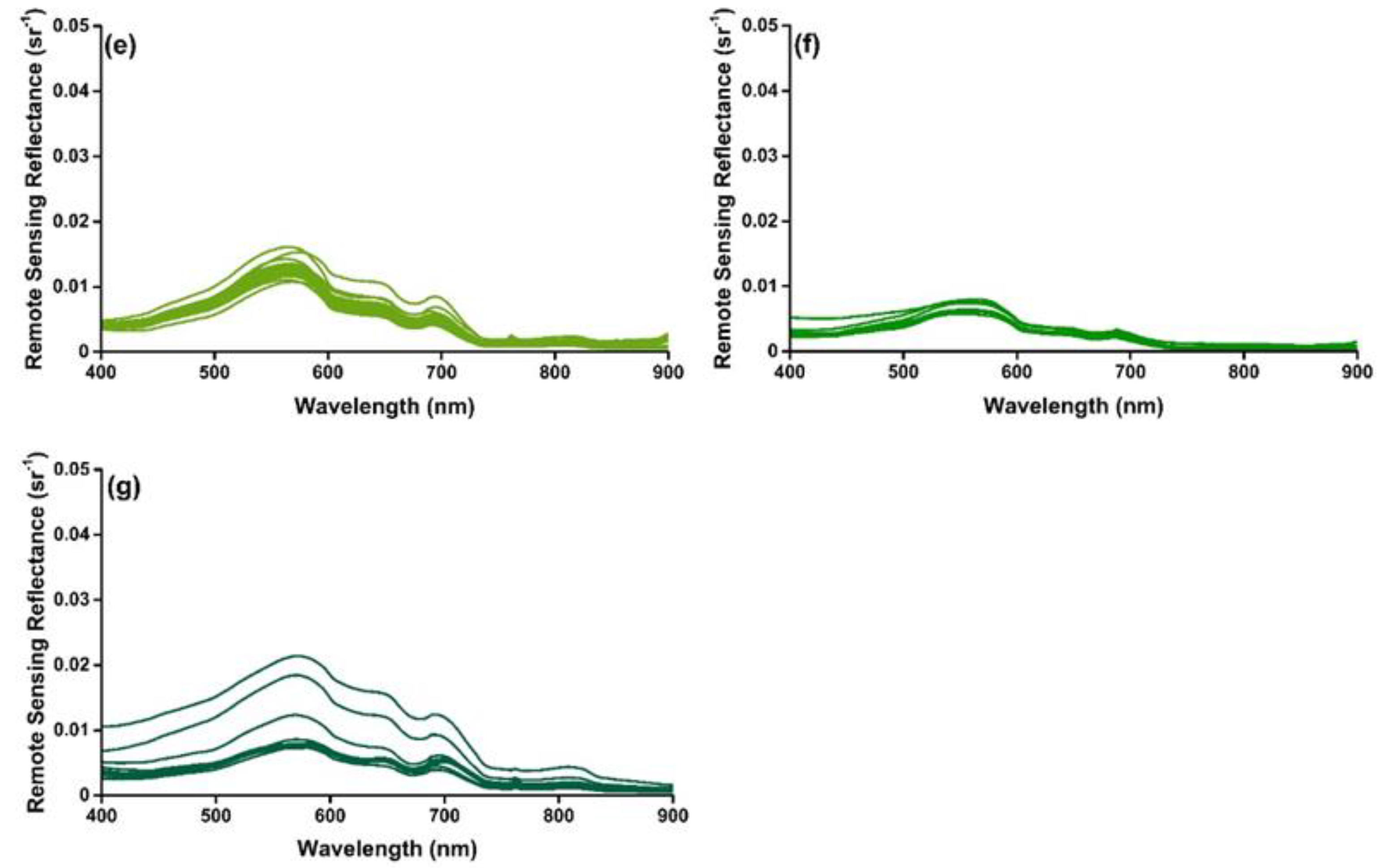
2.2. In Situ Dataset

The field measured dataset includes 112 samplings collected from the seven study areas, which mainly include the remote sensing reflectance R_rs spectrum, Z_sd and turbidity s, as well as the water surface photos taken by mobile phones with reference cards.

In the R_rs measurement, a portable field spectrometer (ASD FieldSpec^®, Analytical Spectral Device, Inc., Boulder, CO, USA) was used at each water surface sampling station following the ‘above water method’ [20]. Using the spectrometer, the radiance of a 30 × 30 cm² reference panel (L_p), the total radiance of the water body (L_w), and the downward radiance of the sky (L_sky) were measured. The total radiance of the water body was measured 10 times at each sampling station. The outliers in the 10 spectra were mostly those affected by sun–glint and were excluded from the dataset. The remaining spectra were averaged to calculate L_w. The equation for calculating the R_rs (remote sensing reflectance) (sr⁻¹) from the measured spectral data is shown in Equation (1). Figure 2 shows the water–leaving reflectance at each of the 112 sampling points in the seven study areas. As there is little difference in the red–green–blue (RGB) spectral response functions of different digital cameras [21], and the factory spectral response function of a smartphone camera is usually not provided, the water–leaving reflectance spectra were simulated as RGB bands using the Canon 50D RGB band response function. The simulated RGB bands from the water–leaving reflectance were used to validate the R_rs values calculated from the RGB bands from the water surface photographs.

R_rs = (L_w − r_sky × L_sky)/(L_p × π/R_p)

(1)

where r_sky is the fraction of skylight reflected by the water surface, which depends on the position of the sun, observation geometry, and water surface roughness. In the ‘above water method’, the viewing direction is about 40° from nadir and the viewing azimuth is about 135° from the plane of the sun. For this observation geometry, and for the relatively low wind speeds observed during the seven experiments, r_sky ≈ 0.028 was regarded as acceptable [22,23]. R_p is the reflectance of the reference panel, which was calibrated in the laboratory.

The Secchi–disk depth (Z_sd) was measured by slowly lowering the black and white Sechi disk into the water and noting the rope scale when the disk became invisible. A portable turbidity meter, AZ8601 (AZ ^® Instrument, Taiwan, China), was calibrated and used to measure the turbidity of the water on site.

Water surface photographs were collected quickly while performing the spectral measurements and water quality parameter measurements in the seven study areas, to avoid solar radiation changes during the experiment. The smartphone models used in the collection of the water surface photographs are shown in

Table 2. Summary of smartphone models used for photography and water quality parameters in the study areas.

Study Area Name	Smartphone Model (Operating System)	Average Zsd (cm)	Standard Deviation of Zsd (cm)	Average Turbidity (NTU)	Standard Deviation of Turbidity (NTU)
Nanfei River	Mi 8 (Android)	38.4	9.8	30.1	21.3
The Summer Palace	Mi 8 (Android)	46.7	2.4	20.3	1.6
Guanting Reservior	Mi 8 (Android)	57.7	9.2	15.6	3.7
Danjiangkou Reservior	Apple XS (Apple)	455.7	85.5	1.2	0.6
Baiguishan Reservior	Apple XS (Apple)	122.2	29.0	5.4	1.9
XiaolangdiReservior	Apple XS (Apple)	245.0	42.0	2.2	0.3
Yuqiao Reservior	Honor9 (Android)	85.5	14.2	8.4	3.7

, together with the water quality parameters in the seven study areas.

3. Methods

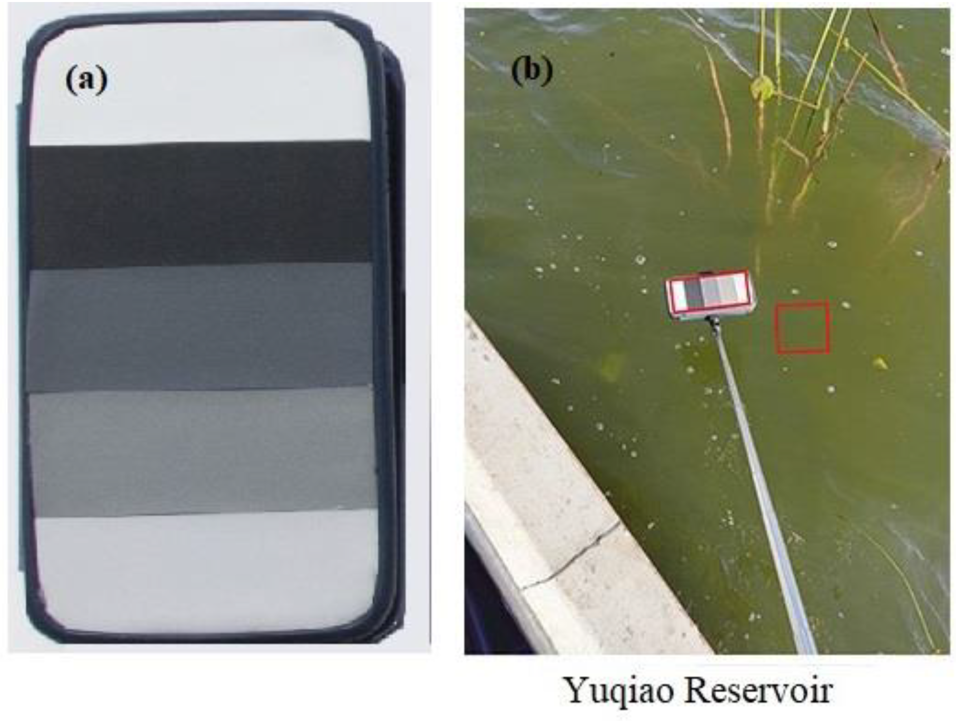
3.1. Water Surface Photographs Taken by Smartphone Camera

3.1.1. Observation Geometry Design

Obtaining water–leaving radiation using a smartphone camera is the same as using the field spectrometer, and solar glint and shore reflectance need to be avoided. Therefore, the observation geometry for the photograph taken using a smartphone camera also followed the above–water spectral observation geometry described in the ocean optic protocol [20]. Briefly, when the photograph is taken, the smartphone camera should be pointing toward the water surface at a viewing zenith angle of 40°–45°, and the viewing azimuth angle should be approximately 135°. Using this observation geometry, the influence of the bidirectionality of the reference card on the inversion results could be significantly avoided.

3.1.2. Five-Color Reference Card

As the exposure parameters of smartphone cameras cannot be controlled, and the exposure time significantly affects the DN values of the photograph, a five-color reference card with specific reflectance was designed in this study and used while taking the water surface photographs. A similar five-color reference card has been used as the target cloth during UAV flight [24] and can minimize bidirectionality. During the water surface photography, the five-color reference card was placed horizontally, close to the water surface in the middle of the photograph view, and the color scale bar of the reference card was pointed forward (Figure 3).

Table 3. Reflectance parameters of each band of the five-color reference card.

	Band	Red Band	Green Band	Blue Band
Reflectance Scale
White card		0.6769	0.6697	0.6458
Bright gray card		0.4824	0.4695	0.4596
Medium gray card		0.1983	0.1973	0.1927
Dark gray card		0.0957	0.0978	0.1005
Black card		0.0312	0.0315	0.0316

shows the reflectance of the five-color reference card in the three visible bands, which was carefully measured and calibrated with spectrometer in an optical laboratory [24]. The specific reflectance of this five-color reference card in the photograph was then used to fit the relationship between the surface reflectance and its DNs, and subsequently to calculate the water reflectance [9].

3.2. R_rs Derivation from Water Surface Photograph

The upward radiance of the water surface is the sum of the water–leaving radiance and the reflected radiance of the sky, within which only the water–leaving radiance contains information about the water constituents. As stated above Equation (1), the R_rs is the ratio of the water–leaving radiance to the downwelling irradiance. However, the water–leaving reflectance in many studies on the inversion of water quality parameters is simply derived by dividing the surface reflectance by π, neglecting the small contribution of skylight reflection [25,26,27]. This study uses the same strategy to calculate the water–leaving reflectance.

3.2.1. Reference Card and Water Body Photograph Clipping

First, a rectangular section of the water body was clipped out, avoiding solar reflections, shadows, and floating objects. Then, the other rectangle that contained the five-color reference card was clipped out. Figure 3b shows the examples for the two clipped rectangles. After clipping, the median DN value in the water body rectangle and the median DN values for the five gray colors in the reference card rectangle were calculated, and the values would be used in subsequent calculations.

3.2.2. Water Reflectance Calculation

According to [8], for current smartphone cameras and ordinary commercial cameras, the GAMMA correction parameters used for converting the incident light intensity to the DNs of the photograph are not uniform, and there are large uncertainties. In this study, the water surface and five-color reference card were photographed at the same time in a single photograph; thus, the downwelling irradiance (E_d) was the same. Hence, a nonlinear model converting the DN values to reflectance, rather than the light intensity or upwelling radiance, was fitted for each water surface photograph, as shown in Equations (2)–(4). Owing to the uncertainties of the GAMMA correction, the nonlinear response between the reflectance and photograph DN values of the five-color reflectance reference card was first fitted using either the power function model or the E–index model. Then, the model coefficients a, b, c, and d were derived using the DN values of the five-color reference card and their interior reflectance. The final model was determined by comparing the R² values of the two models. The determined model was further used to obtain the water reflectance (R_w) using the median DN value of the water surface photograph. Finally, R_rs was calculated by dividing the derived water reflectance by π, as shown in Equation (4).

$$R=\mathrm{a}\times { \mathrm{DN}}^{\mathrm{b}}$$

(2)

$$R=\mathrm{c}\times \exp \left(\mathrm{d}\times \mathrm{DN}\right)$$

(3)

$$R_{rs}=R_w/\mathsf{\pi }$$

(4)

where R is the specific reflectance of the five-color reference card. DN is the digital value of the five-color reference card in the photography. R_w represents water reflectance calculated using the determined R–DN model. a, b, c, and d are the fitted model coefficients.

3.3. Water Quality Retrieval

Turbidity and Secchi–disk depth are two quantitative indicators of the turbidity of lake water. Commonly used water quality parameter inversion methods mainly include analytical/semi–analytical methods, empirical/semi–empirical methods, and machine learning algorithms. To preliminarily test the effectiveness of water quality parameter inversion from automatically exposed water surface photographs taken using smartphones, several empirical/semi–empirical algorithms were tested. Thus, relatively simple empirical/semi–empirical methods are used for the inversion modeling analysis in this study, such as the RGB band reflectance, reflectance band ratio, reflectance band difference, and chromaticity angle [19]. For two–thirds (N = 76) of all the water surface sampling points across the seven study areas (randomly chosen), the least squares method was used to establish the mathematical statistical analysis models, such as linear regression, exponential/logarithmic function regression, and polynomial regression [28,29]. The reserved 1/3 (N = 36) water sample points was used to validate the established water quality parameter models.

3.4. Accuracy Evaluation

To evaluate the model accuracy, this study used the root mean square error (RMSE), the average unbiased relative error (AURE), the coefficient of determination (R²), and the average ratio between the calculated and measured values (hereafter the accuracy ratio) [30], as accuracy evaluation indices. Thereinto, the RMSE indicated the absolute errors, the AURE indicated the relative errors, the R² indicated the goodness of the fitting, and the accuracy ratio indicated the ratio of the straight line fitted to the measured data. These indices can be calculated using the equations as follows:

$$\mathrm{RMSE}=\sqrt{{{\displaystyle \sum }}_{\mathrm{i}=1}^N{\left(Xi-xi\right)}^2/N}$$

(5)

$$\mathrm{AURE}={{\displaystyle \sum }}_{\mathrm{i}=1}^N\left(\frac{\left|Xi-xi\right|}{\left(Xi+xi\right)/2}\right)/N$$

(6)

$${\mathrm{R}}^2=1-\frac{{{\displaystyle \sum }}_{\mathrm{i}}{\left(Xi-xi\right)}^2}{{{\displaystyle \sum }}_{\mathrm{i}}{\left(\overline{x}-xi\right)}^2}$$

(7)

$$\mathrm{Accuracy} \mathrm{ratio}={{\displaystyle \sum }}_{\mathrm{i}=1}^{N}Xi/xi/N$$

(8)

where Xi represents the modelled value; xi represents the field measured data; $\overline{x}$ represents mean measured data; N refers to the number of sampling stations.

4. Results

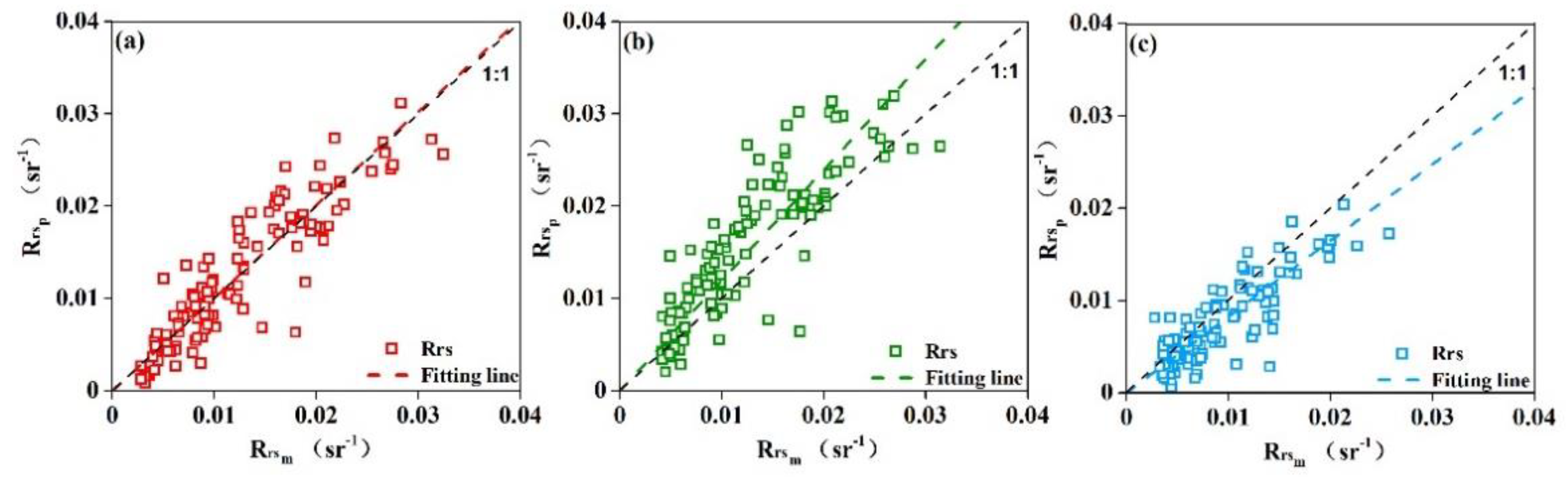
4.1. Validation of Smartphone Photograph–Derived R_rs

The DN values of the waterbodies at the 112 sampling points and their associated reference cards were calculated as R_rs using Equations (2)–(4), based on the water surface photographs derived from a reference card–assisted smartphone camera with automatic exposure parameters. Scatterplots of the R_rs obtained from the digital photographs and the equivalent water–leaving reflectance measured by the spectrometer are shown in Figure 4. The accuracy evaluation parameters (RMSE, AURE, R², and the accuracy ratio) are shown in

Table 4. Retrieval accuracy of water reflectance from 112 sampling–point photographs.

Band	RMSE (sr−1)	AURE (%)	R2	Accuracy Ratio
Red	0.0032	25.7	0.98	0.98
Green	0.0051	29.5	0.94	1.20
Blue	0.0031	35.2	0.92	0.80

. The accuracy of reflectance is high, R² is between 0.92 and 0.98, AURE is between 25.7 and 35.2%, and the accuracy ratio is between 0.80 and 1.20.

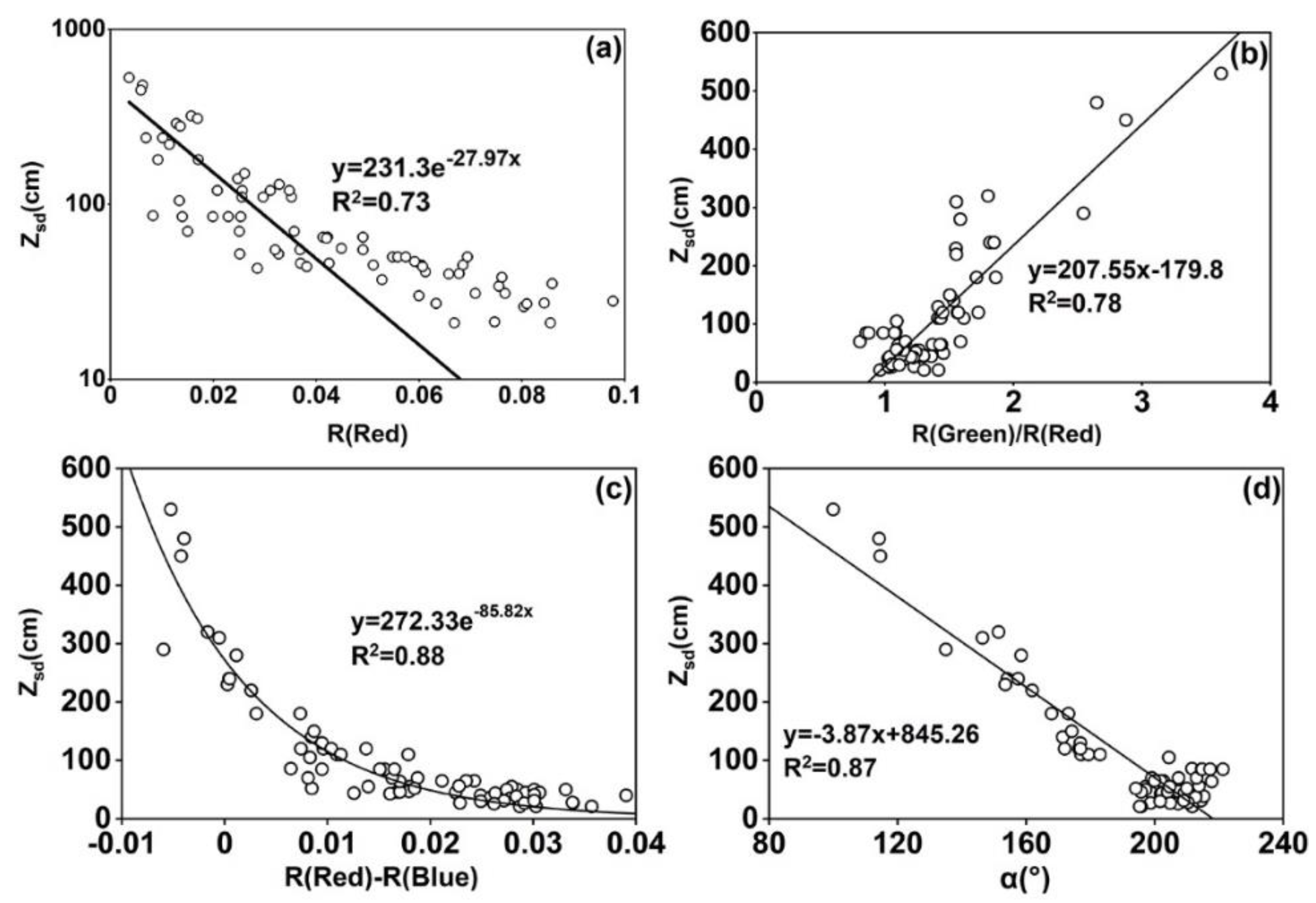
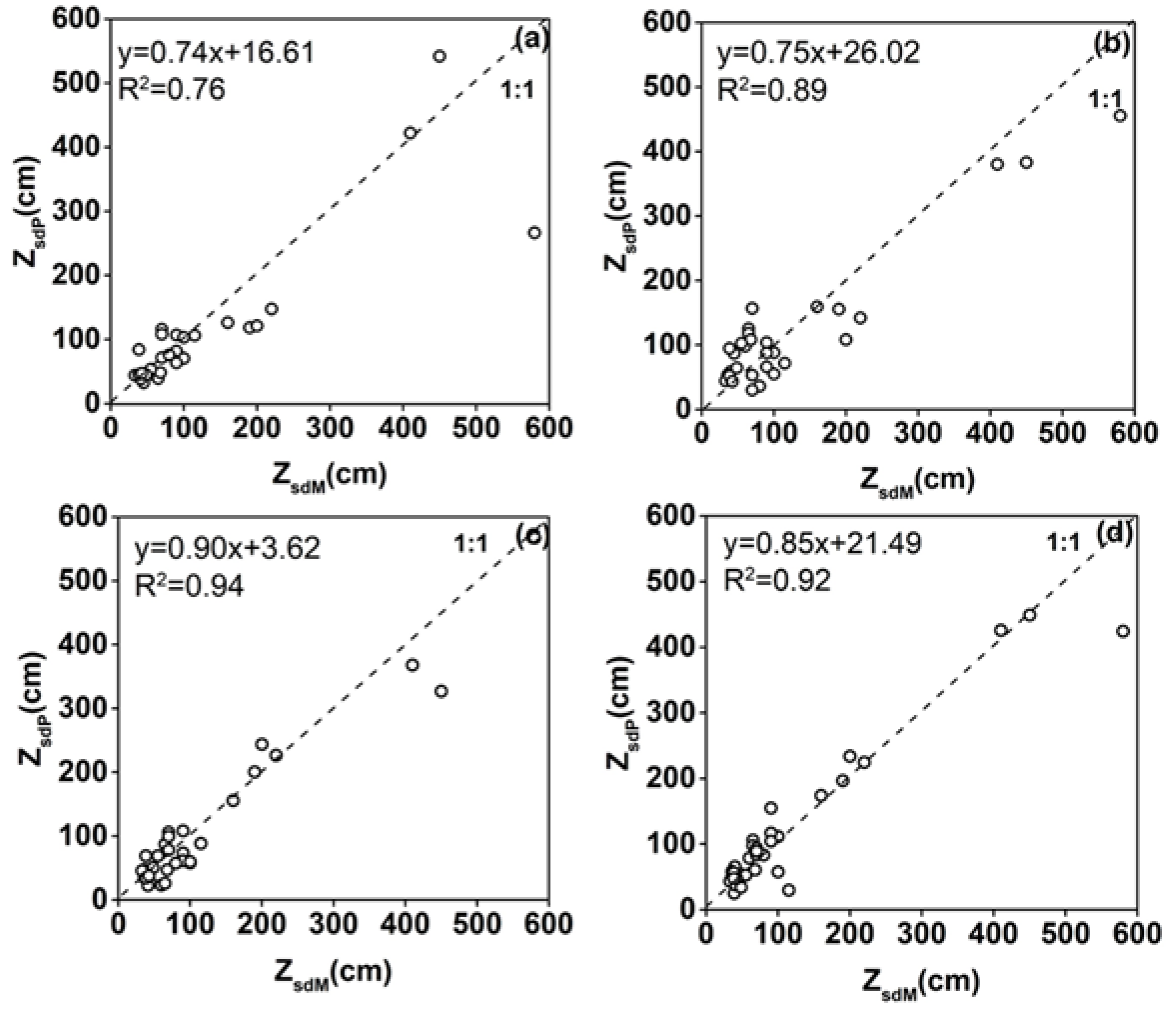
4.2. Secchi–Disk Depth Estimation Based on Smartphone Photography

With R_rs derived from the smartphone photos, several frequently used Z_sd models were tested using the in situ dataset. Figure 5 shows four outperformed models, including the logarithmic model of the red band, the linear model of the green:red band ratio, the e–index model of the difference between the red and blue bands, and the linear model of the chromaticity angle. Figure 6 shows scatterplots using the remaining 36 sampling points to test the four models.

Table 5. Z_sd model accuracy test.

Zsd Inversion Model Name	AURE (%)	Accuracy Ratio	R2
(a) Red band model	25.5	0.74	0.76
(b) Green:red band ratio model	37.5	0.75	0.89
(c) Red and blue band difference model	27.6	0.90	0.94
(d) Chromaticity angle model	27.0	0.85	0.92

compares the accuracy evaluation indicators of the four models. In a comprehensive analysis of the accuracy indicators, the Z_sd inversion model based on the difference between the red and blue bands was the best–performing model. The inversion model is shown in Equation (9). The fitting R² was 0.88, calculated based on the modeling data (N = 76). The R² between the calculated Z_sd inversion results and the measured values was 0.94, based on the validation data (N = 36), and the unbiased relative error was 27.6%.

$$Z_{sd}=231.33\times \exp \left(-85.82\times \left(R-\mathrm{B}\right)\right)$$

(9)

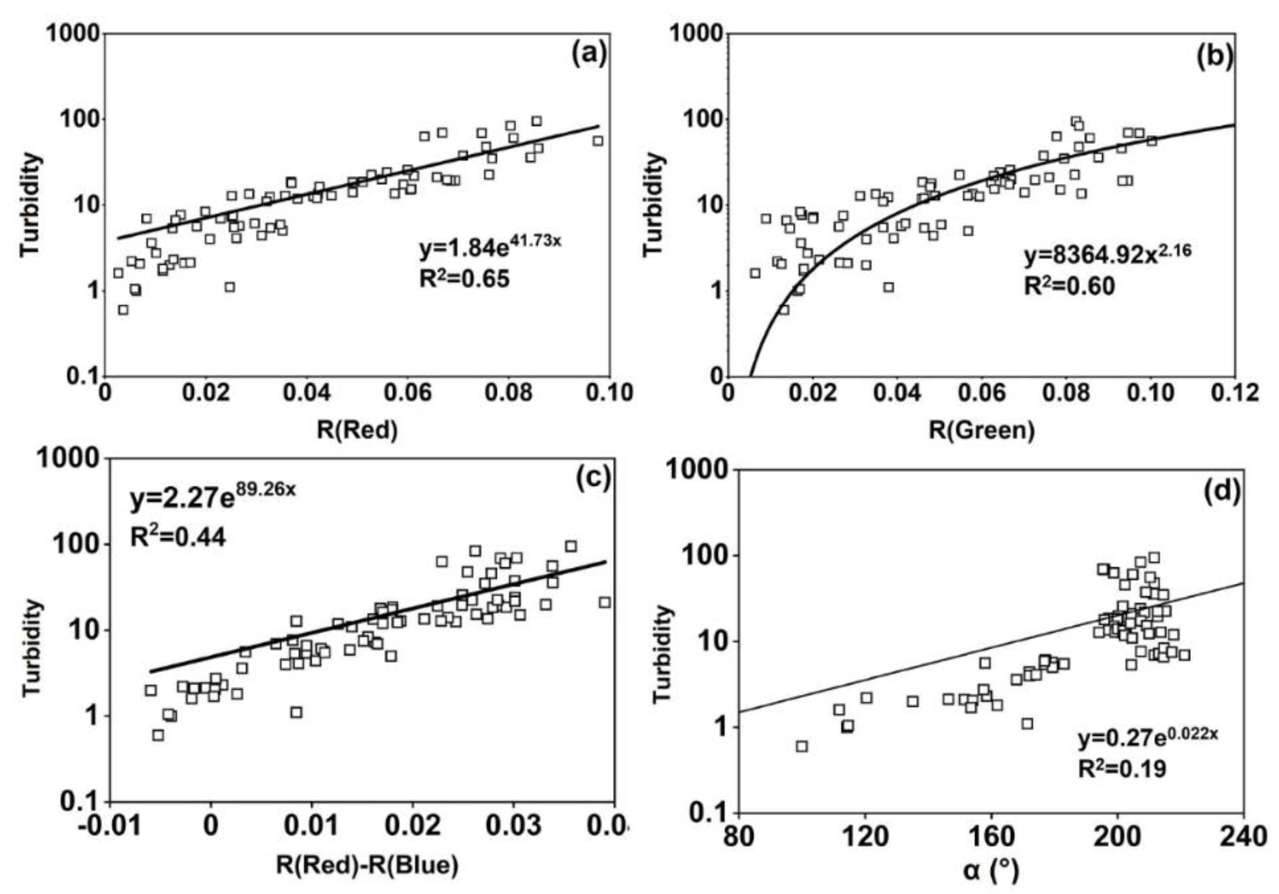
4.3. Turbidity Estimation Based on Smartphone Photography

Turbidity is an important water quality parameter in river water environment monitoring, and it has a close relationship with suspended solids. The analysis of turbidity changes is helpful for understanding the distribution of total suspended solids or sediments in waterbodies and can provide effective information for studying the behavior of pollutant sedimentation, decomposition, and diffusion in waterbodies. Therefore, monitoring the spatial distribution of turbidity is of great significance for water pollution control [31].

With R_rs derived from the smartphone photos, several frequently used turbidity models were tested using the in situ dataset. Figure 7 shows four outperformed models, including the models based on red band, green band, red–blue band difference, and chromaticity angle. Figure 8 shows scatterplots for the validation of these four models.

Table 6. Turbidity model accuracy test.

Turbidity Inversion Model Name	AURE (%)	Accuracy Ratio	R2
(a) Red band model	39.8	0.99	0.61
(b) Green band model	50.5	0.91	0.32
(c) Red and blue band difference model	35.7	0.82	0.57
(d) Chromaticity angle model	31.9	0.62	0.61

shows a comparison of the accuracy evaluation indicators of the models. After a comprehensive analysis of the various indicators, the turbidity inversion model based on the difference between the red and blue bands was the best, as shown in Equation (10). Based on the modeling data (N = 76), the calculated fitting R² was 0.65. The R² between the turbidity inversion results calculated based on the validation data (N = 36) was 0.61, and the unbiased relative error was 39.8%.

$$\mathrm{Turbidity}=1.84\times \exp \left(41.73\times R\right)$$

(10)

5. Discussion on the Uncertainties Caused by Smartphone Parameter Settings

In this study, a smartphone–based method for calculating water–leaving reflectance was constructed. It was applied to the inversion of typical water quality parameters and achieved good results. The next step is to integrate these methods into a mobile app. In our calculations, we did not consider the influence of the parameter settings of the smartphone, such as spectral response function and the white balance. The parameter settings of different mobile phone cameras may cause calculation errors. Therefore, in this section, we further explore and discuss the influence of some smartphone parameter settings, including the influence of the spectral response function of different cameras and the white balance.

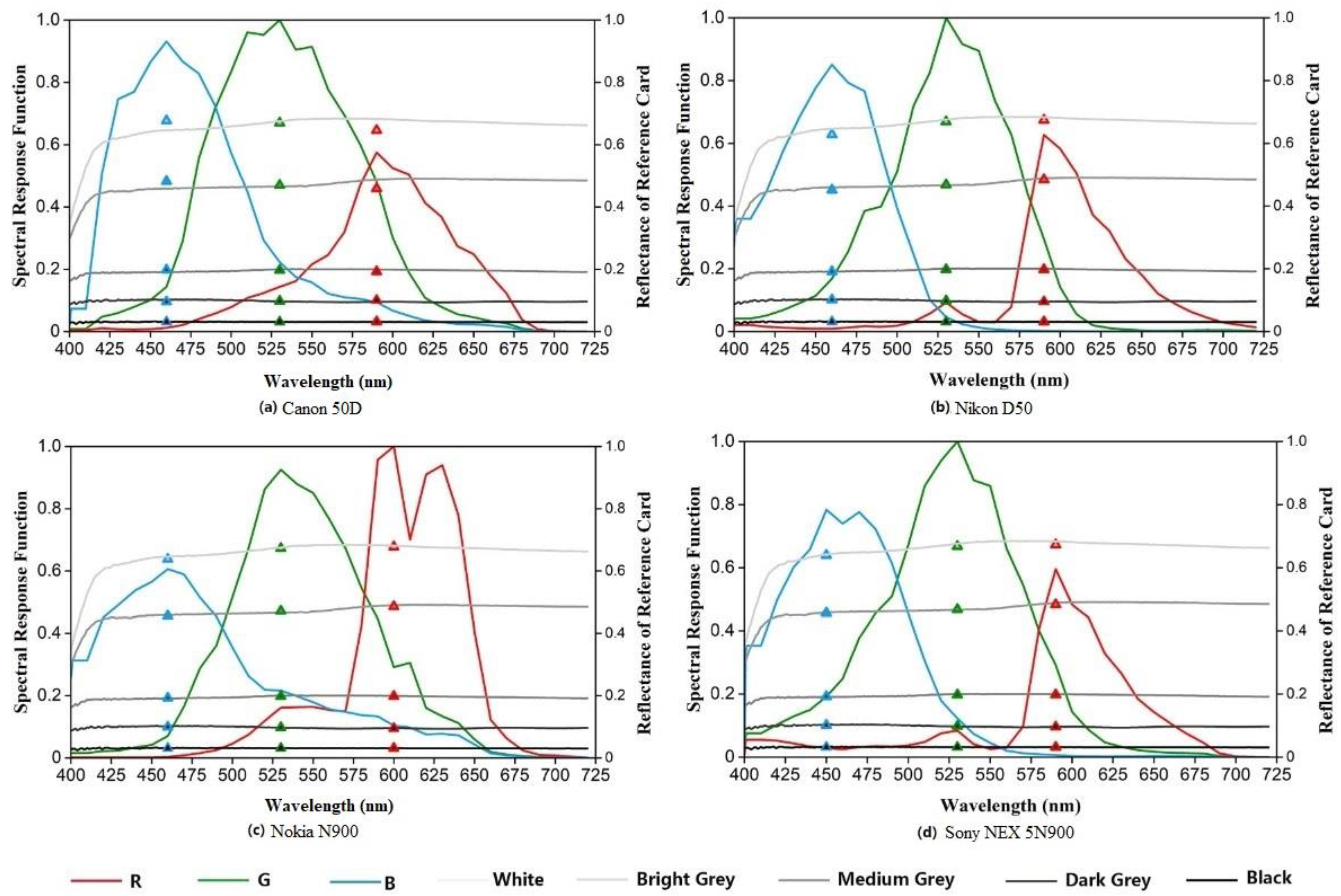
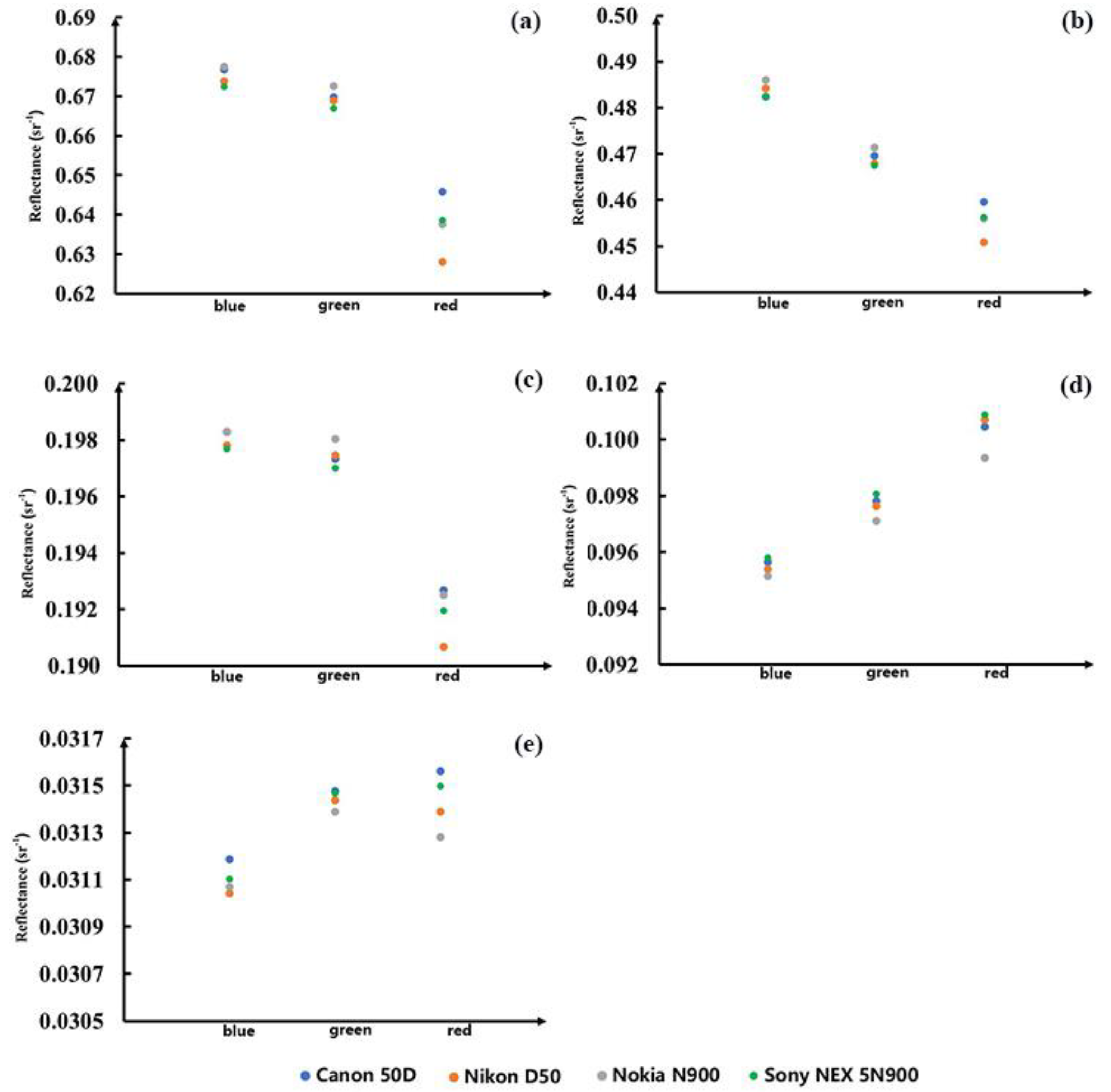
5.1. Uncertainties Caused by the Spectral Response Functions of Different Digital Cameras

There are two main water surface photograph collection devices in daily life: mobile phones and cameras. Mobile phones are divided into Android and Apple phones. Because of the photosensitive elements in the cameras, they have specific wavelength response ranges, namely, the spectral response function. Different cameras have different spectral response functions. Figure 9 shows the spectral response function curves of four cameras [21], together with the reflectance curve of the five-color reference card used in the experiment, and the equivalent results of the spectral response functions of the four cameras. It showed that the spectral response functions of the Canon 50D camera, Nikon D50 camera, and Sony NEX 5N900 camera were very similar across all bands. The red band of the Nokia N900 camera has an additional peak at 630 nm. To further quantify the differences of the four cameras, the reflectance spectra of the five-color reference card used in the study is equivalent to the blue, green, and red bands using the spectral response function of the cameras. Figure 10 shows the equivalent spectral reflectance values on the three visible bands for the five-color reference card from the four cameras. It was found that the results for the four cameras were almost the same. Therefore, the uncertainty in the water–leaving reflectance values introduced by using different cameras is relatively small. This is similar to the conclusion drawn in [32]. To further confirm this, the blue, green and red band reflectance of the 4 digital cameras were equivalent from the spectrum measured by the field spectrometer in Nanfei River according to the four cameras’ spectral response function. Taking the three bands’ equivalent value of the Canon 50D camera as the true value, the calculated average errors of the other cameras for the red, green, and blue bands were 1.66%, 2.46%, and 7.10%, respectively. This indicates that the uncertainty caused by the spectral response functions of different digital cameras is generally small (<10%), as the cameras are basically designed to capture the same color as that seen by the human eye, so their spectral response functions do not differ significantly.

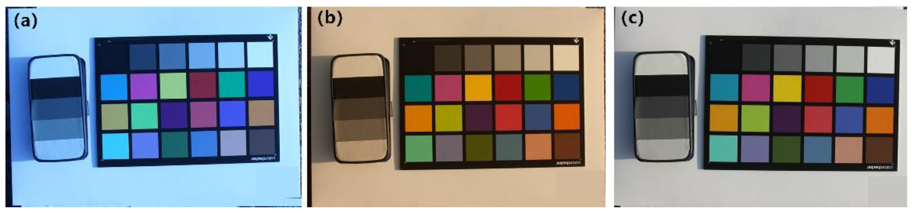
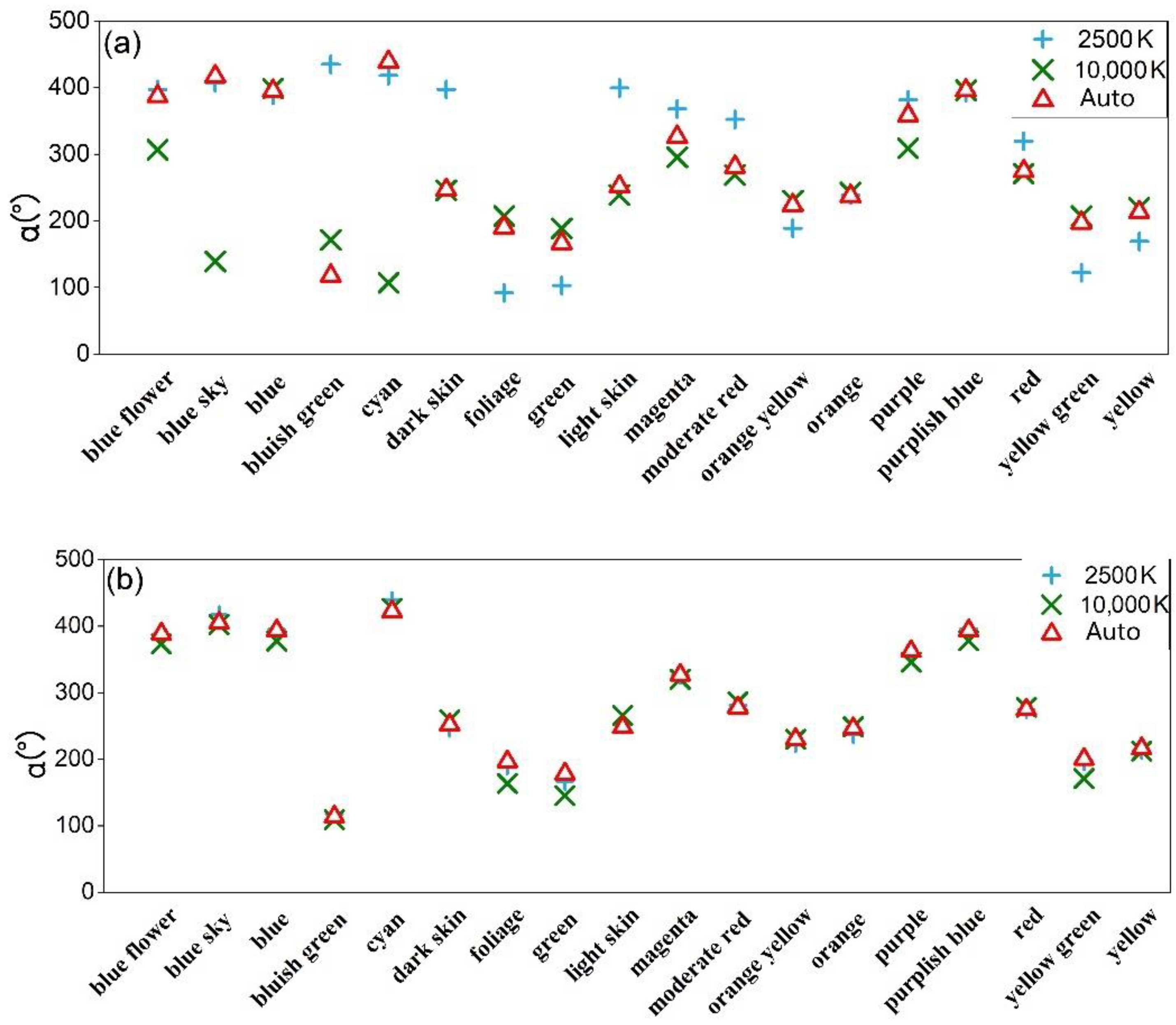
5.2. Uncertainties Caused by the Automatic White Balance

Different light sources have different spectral characteristics, which are called color temperatures in optics. As they are affected by the light source, white objects tend to be reddish at low color temperatures and bluish at high color temperatures. The human eye can correct our vision, automatically adjusting for the color deviation caused by different color temperatures and ensuring color constancy. If the camera cannot adjust its white balance with the color temperature of the scene light, it will lead to a color cast. Color cast refers to the color in the photograph, which is obviously different from the real color, with an overall bias towards one color. The white balance is used to adjust the color circuit inside the camera to offset color casts in images taken under different color temperature conditions, similar to the adjustments made by the human eye [33,34].

To study the effect of the white balance on the calculation of water reflectance in photographs, this study used a Canon 50D camera, set the camera’s white balance to 2500 K, 10,000 K, and automatic white balance, and captured images of a color card and the five-color reference card (Figure 11). The chromaticity angles of the corresponding color cards in the photographs with severe color casts were calculated using the DN value and the R_rs, after correction using the five-color reference card. As shown in Figure 12, the chromaticity angles calculated from the DN values of the photographs with severe color casts differed significantly from the chromaticity angles calculated from the automatic white balance DN values. When the five-color reference card was used to correct the reflectance of the color card in the photographs with serious color casts, the angle difference decreased, indicating that the five-color reference card can be used to reduce the effects of the different white balance algorithms of different devices or insufficient white balance.

6. Conclusions

This study focused on the calculation of reflectance based on digital water surface photographs and the inversion of typical water quality parameters, including water reflectance, based on smartphone photographs taken with automatic exposure. The main findings and conclusions obtained are outlined in the following two sections.

6.1. Calculation of Water Reflectance Based on Digital Photographs of the Water Surface

Because smartphone applications cannot usually control the exposure parameters of the camera, photographs can only be taken in automatic exposure mode. Therefore, this study developed a set of water reflectance correction methods based on smartphones with automatic exposure parameters: First, when photographing the water surface, five different reflectance references (combined into a five-color reference card) were simultaneously captured in the photograph. The five-color reference card was then used to fit the nonlinear relationship between reflectance and the DNs of the photograph. The water reflectance could then be calculated, ignoring the sky light correction. The water surface reflectance spectra of 112 sampling points obtained from experiments in seven study areas, including Nanfei River and Guanting Reservoir, were used to test the water reflectance results extracted from synchronous photographs. The average relative errors of the red, green, and blue bands were 24.5%, 35.5%, and 30.4%, respectively, and the R² were 0.98, 0.94, 0.92, indicating that the accuracy of this method is relatively high.

6.2. Inversion of Water Quality Parameters by Calculating Water Reflectance Based on Smartphone Water Surface Photographs

In this study, typical water quality parameter inversion models of water reflectance were constructed, based on smartphone photographs: First, we compared the statistical relationships between four spectral indices (single–band, band ratio, band difference, and chromaticity angle) of water reflectance calculated from the smartphone photographs and two typical water quality parameters (Z_sd and turbidity) measured in seven study areas, to obtain the most accurate models. It was found that the model based on the difference between red and blue bands was the best performing for Z_sd estimation and the model based on the red band was the best performing for turbidity estimation. Second, these two models were verified using the reserved 36 sampling points. The errors of the Z_sd and turbidity models were 27.6% and 39.8%, respectively, and the R² values were 0.94 and 0.57, indicating that the method proposed in this paper is reliable for the retrieval of water quality parameters from smartphone photographs.

References

1. Zhang, B.; Li, J.; Shen, Q.; Wu, Y.; Zhang, F.; Wang, S. Key Technologies and Systems of Surface Water Environment Monitoring by Remote Sensing. Environ. Monit. China 2019, 35, 1–9. [Google Scholar]
2. Barwick, H. The ‘Four Vs’ of Big Data. In Proceedings of the Implementing Information Infrastructure Symposium, Sydney, Australia, 5 August 2011. [Google Scholar]
3. Beyer, M.A.; Laney, D. The Importance of ‘Big Data’: A Definition; Gartner: Stamford, CT, USA, 2012. [Google Scholar]
4. Liang, D.; Wang, L.; Chen, F.; Guo, H. Scientific big data and digital Earth. Chin. Sci. Bull. 2014, 59, 1047–1054. (In Chinese) [Google Scholar] [CrossRef]
5. Wu, B.; Zhang, M.; Zeng, H.; Zhang, X.; Yan, N.; Meng, J. Agricultural Monitoring and Early Warning in the Era of Big Data. J. Remote Sens. 2016, 20, 1027–1037. [Google Scholar]
6. Leeuw, T. Crowdsourcing Water Quality Data Using the iPhone Camera. Master’s Thesis, The University of Maine, Orono, ME, USA, 2014. [Google Scholar]
7. Leeuw, T.; Boss, E. The HydroColor App: Above Water Measurements of Remote Sensing Reflectance and Turbidity Using a Smartphone Camera. Sensors 2018, 18, 256. [Google Scholar] [CrossRef] [PubMed] [Green Version]
8. Burggraaff, O.; Schmidt, N.; Zamorano, J.; Pauly, K.; Pascual, S.; Tapia, C.; Spyrakos, E.; Snik, F. Standardized Spectral and Radiometric Calibration of Consumer Cameras. Opt. Express 2019, 27, 19075–19101. [Google Scholar] [CrossRef] [Green Version]
9. Gao, M.; Li, J.; Zhang, F.; Wang, S.; Xie, Y.; Yin, Z.; Zhang, B. Measurement of Water Leaving Reflectance Using a Digital Camera Based on Multiple Reflectance Reference Cards. Sensors 2020, 20, 6580. [Google Scholar] [CrossRef]
10. Malthus, T.J.; Ohmsen, R.; van der Woerd, H.J. An Evaluation of Citizen Science Smartphone Apps for Inland Water Quality Assessment. Remote Sens. 2020, 12, 1578. [Google Scholar] [CrossRef]
11. Salama, M.; Mahama, P. Smart Phones for Water Quality Mapping. Master’s Thesis, University of Twente, Enschede, The Netherlands, 2016. [Google Scholar]
12. Liu, D.; Duan, H.; Loiselle, S.; Hu, C.; Zhang, G.; Li, J.; Yang, H.; Thompson, J.R.; Cao, Z.; Shen, M.; et al. Observations of Water Transparency in China’s Lakes from Space. Int. J. Appl. Earth Obs. Geoinf. 2020, 92, 102187. [Google Scholar] [CrossRef]
13. Lathrop, R.G., Jr.; Lillesand, T.M. Monitoring Water Quality and River Plume Transport in Green Bay, Lake Michigan with SPOT–1 Imagery. Photogramm. Eng. Remote Sens. 1989, 55, 349–354. [Google Scholar]
14. Binding, C.E.; Jerome, J.H.; Bukata, R.P.; Booty, W.G. Trends in Water Clarity of the Lower Great Lakes from Remotely Sensed Aquatic Color. J. Great Lakes Res. 2007, 33, 828–841. [Google Scholar] [CrossRef] [Green Version]
15. Olmanson, L.G.; Bauer, M.E.; Brezonik, P.L. A 20-Year Landsat Water Clarity Census of Minnesota’s 10,000 Lakes. Remote Sens. Environ. 2008, 112, 4086–4097. [Google Scholar] [CrossRef]
16. Song, T.; Shi, J.; Liu, J.; Xu, W.; Yan, F.; Xu, C.; Zhu, B. Research on Remote Sensing Quantitative Inversion Models of Blue–green Algae Density and Turbidity Based on Landsat–8 OLI Image Data in Lake Taihu. Saf. Environ. Eng. 2015, 22, 67–71, 78. (In Chinese) [Google Scholar]
17. Wang, S.; Li, J.; Shen, Q.; Zhang, B.; Zhang, F.; Lu, Z. MODIS-Based Radiometric Color Extraction and Classification of Inland Water with the Forel–Ule Scale: A Case Study of Lake Taihu. IEEE J. Sel. Top. Appl. Earth Obs. Remote Sens. 2015, 8, 907–918. [Google Scholar] [CrossRef]
18. Wang, S.; Li, J.; Zhang, B.; Lee, Z.; Spyrakos, E.; Feng, L.; Liu, C.; Zhao, H.; Wu, Y.; Zhu, L.; et al. Changes of Water Clarity in Large Lakes and Reservoirs Across China Observed from Long–Term MODIS. Remote Sens. Environ. 2020, 247, 111949. [Google Scholar] [CrossRef]
19. Wang, S.; Li, J.; Zhang, B.; Spyrakos, E.; Tyler, A.N.; Shen, Q.; Zhang, F.; Kuster, T.; Lehmann, M.K.; Wu, Y.; et al. Trophic State Assessment of Global Inland Waters Using a MODIS–Derived Forel–Ule Index. Remote Sens. Environ. 2018, 217, 444–460. [Google Scholar] [CrossRef] [Green Version]
20. Mueller, J.; Fargion, G. Ocean Optics Protocols for Satellite Ocean Color Sensor Validation, Revision 3; NASA: Washington, DC, USA, 2003; Volume 2. [Google Scholar]
21. Prasad, D.; Nguyen, R.; Brown, M. Quick Approximation of Camera’s Spectral Response from Casual Lighting. In Proceedings of the IEEE International Conference on Computer Vision (ICCV) Workshops, Sydney, Australia, 2–8 December 2013; pp. 844–851. [Google Scholar]
22. Mobley, C.D. Estimation of the Remote–Sensing Reflectance from Above-Surface Measurements. Appl. Opt. 1999, 38, 7442–7455. [Google Scholar] [CrossRef]
23. Mobley, C.D. Polarized Reflectance and Transmittance Properties of Windblown Sea Surfaces. Appl. Opt. 2015, 54, 4828–4849. [Google Scholar] [CrossRef]
24. Xu, W.; Zhang, L.; Yang, B.; Qiao, Y. On–orbit radiometric calibration based on gray-scale tarps. Acta Opt. Sin. 2012, 32, 164–168. [Google Scholar]
25. Shenglei, W.; Junsheng, L.; Bing, Z.; Qian, S.; Fangfang, Z.; Zhaoyi, L. A Simple Correction Method for the MODIS Surface Reflectance Product Over Typical Inland Waters in China. Int. J. Remote Sens. 2016, 37, 6076–6096. [Google Scholar] [CrossRef]
26. Yin, Z.; Li, J.; Huang, J.; Wang, S.; Zhang, F.; Zhang, B. Steady Increase in Water Clarity in Jiaozhou Bay in the Yellow Sea From 2000 to 2018: Observations From MODIS. J. Ocean. Limnol. 2021, 39, 800–813. [Google Scholar] [CrossRef]
27. Yin, Z.; Li, J.; Liu, Y.; Xie, Y.; Zhang, F.; Wang, S.; Sun, X.; Zhang, B. Water Clarity Changes in Lake Taihu Over 36 Years Based on Landsat TM and OLI Observations. Int. J. Appl. Earth Obs. Geoinf. 2021, 102, 102457. [Google Scholar] [CrossRef]
28. Duan, H.T.; Wen, Y.; Zhang, B.; Song, K.S.; Wang, Z.M. Application Hyperspectral Data in Remote Sensing Inverse of Water Quality Variables in Lake Chagan. J. Arid. Land Resour. Environ. 2006, 20, 104–108. [Google Scholar]
29. Koponen, S.; Pulliainen, J.; Kallio, K.; Hallikainen, M. Lake Water Quality Classification with Airborne Hyperspectral Spectrometer and Simulated MERIS Data. Remote Sens. Environ. 2002, 79, 51–59. [Google Scholar] [CrossRef]
30. Wang, M.; Son, S.; Zhang, Y.; Shi, W. Remote Sensing of Water Optical Property for China’s Inland Lake Taihu Using the SWIR Atmospheric Correction With 1640 and 2130–nm Bands. IEEE J. Sel. Top. Appl. Earth Obs. Remote Sens. 2013, 6, 2505–2516. [Google Scholar] [CrossRef]
31. Xiao, X.; Xu, J.; Zhao, D.Z.; Zhao, B.C.; Xu, J.; Cheng, X.J.; LI, G.Z. Research on Combined Remote Sensing Retrieval of Turbidity for River Based on Domestic Satellite Data. J. Yangtze River Sci. Res. Inst. 2021, 38, 128. [Google Scholar]
32. Goddijn-Murphy, L.M.; Dailloux, D.; White, M.; Bowers, D. Fundamentals of In Situ Digital Camera Methodology for Water Quality Monitoring of Coast and Ocean. Sensors 2009, 9, 5825–5843. [Google Scholar] [CrossRef] [PubMed]
33. Wang, Z.C.; Yin, Y. Underwater Image Enhancement Based on Color Balance and Correction. Ship Sci. Technol. 2021, 43, 154–159. [Google Scholar]
34. Wu, X. Sensitivity, White Balance and Shutter Speed in Photography. View Financ. 2021, 4, 82–83. [Google Scholar]
Figure 1. Distribution maps of sampling points in smartphone water quality monitoring experiment, based on automatic exposure.
Remotesensing 14 01371 g001
Figure 2. Remote sensing reflectance spectra measured with a field spectrometer at 117 sampling points at: (a) Nanfei River, (b) The Summer Palace, (c) Guanting Reservoir, (d) Danjiangkou Reservior, (e) Baiguishan Reservoir, (f) Xiaolangdi Reservoir, and (g) Yuqiao Reservoir.
Remotesensing 14 01371 g002aRemotesensing 14 01371 g002b
Figure 3. (a) The five-color reference card used in this study. (b) Sample image of five-color reference card and water taken using a smartphone with automatic exposure parameters. The red box indicates the position of the uniform area clipped.
Remotesensing 14 01371 g003
Figure 4. Scatterplots of water reflectance derived from digital images and measured by spectrometer at 112 sampling stations in (a) red, (b) green, and (c) blue bands.
Remotesensing 14 01371 g004
Figure 5. Models between measured Zsd and (a) red band reflectance, (b) the green:red band ratio, (c) red and blue band difference, and (d) chromaticity angle.
Remotesensing 14 01371 g005
Figure 6. Scatterplots of measured Zsd and model estimated Zsd using (a) red band reflectance, (b) the green:red band ratio, (c) red and blue band difference, and (d) chromaticity angle.
Remotesensing 14 01371 g006
Figure 7. Models between measured turbidity and (a) red band reflectance, (b) green band reflectance, (c) red and blue band difference, and (d) chromaticity angle.
Remotesensing 14 01371 g007
Figure 8. Scatterplots of measured turbidity and model estimated turbidity using (a) red band reflectance, (b) green band reflectance, (c) red and blue band difference, and (d) chromaticity angle.
Remotesensing 14 01371 g008
Figure 9. Spectral response functions of four cameras [21]. (ad) showing the RGB bands (red, green, and blue curves), the reflectance curves of the five-color reference cards (white, bright gray, medium gray, dark gray, and black curves), and the results of the equivalent reflectance of the reference cards in the Canon 50D RGB bands (triangles).
Remotesensing 14 01371 g009
Figure 10. Equivalent reflectance values on the blue, green, red bands for the five-color reference card. (a) White card, (b) bright gray card, (c) medium gray card, (d) dark gray card, and (e) black card from four cameras.
Remotesensing 14 01371 g010
Figure 11. Photographs of color cards for color temperature assessment at 2500 K (a), 10,000 K (b), and using the automatic white balance function (c).
Remotesensing 14 01371 g011
Figure 12. Comparison of chromaticity angle at color temperatures of 2500 and 10,000 K (a) before correction and (b) after correction with the five-color reference card.
Remotesensing 14 01371 g012