SDTGAN: Generation Adversarial Network for Spectral Domain Translation of Remote Sensing Images of the Earth Background Based on Shared Latent Domain

Abstract

The synthesis of spectral remote sensing images of the Earth’s background is affected by various factors such as the atmosphere, illumination and terrain, which makes it difficult to simulate random disturbance and real textures. Based on the shared latent domain hypothesis and generation adversarial network, this paper proposes the SDTGAN method to mine the correlation between the spectrum and directly generate target spectral remote sensing images of the Earth’s background according to the source spectral images. The introduction of shared latent domain allows multi-spectral domains connect to each other without the need to build a one-to-one model. Meanwhile, additional feature maps are introduced to fill in the lack of information in the spectrum and improve the geographic accuracy. Through supervised training with a paired dataset, cycle consistency loss, and perceptual loss, the uniqueness of the output result is guaranteed. Finally, the experiments on the Fengyun satellite observation data show that the proposed SDTGAN method performs better than the baseline models in remote sensing image spectrum translation.

1. Introduction

Remote sensing images are widely used in environmental monitoring, remote sensing analysis, and target detection and classification. However, in practical applications, it is difficult to obtain multi-spectral remote sensing data, especially high-resolution infrared remote sensing data, and spectrally poor data may be available for longer periods of time than spectrally rich data [1]. Many researchers have explored the acquisition of demanded spectral remote sensing images based on simulation methods [2,3,4]. The spectral characteristics are determined by the optical characteristics of the underlying surface type, atmosphere, sunlight, and terminal sensors [5]. The traditional methods based on radiation transfer models [6,7,8] require pre-building a large database of ground features and environmental characteristics. However, it is still difficult to model the complex and random atmosphere and clouds. When the input condition is insufficient for simulating the images of earth background, based on the correlation between the spectral domains, the known spectral images can be used to achieve target spectral image synthesis [9,10,11]. However, the correlation between the spectral domains is implicit and non-linear.

As deep learning technology can obtain feature correlations in complex spaces through a large amount of data to realize end-to-end image generation, generative adversarial networks (GAN) have achieved rapid development in recent years [12], from the initial supervised image translation [13,14,15] to the subsequent unsupervised image translation [16] and the later multi-modal image translation [17]. Domain adaptation is critical for the successful application of neural network models in new, unseen environments [18]. Many tasks that support translation from one domain to another have achieved excellent results. Spectral domain translation refers to generating an image of the target spectral do-main based on the image of the source spectral domain while ensuring that each pixel of the generated image conforms to the physical mapping relationship. In the field of spectral imaging, super-resolution [19], spectral reconstruction [20,21], and spectral fusion [22,23] have successively adopted the GAN technology. Rongxin Tang et al. [24] used generative adversarial networks to achieve RGB visualization through hyperspectral images. The method reduces the dimensionality of the spectral data from tens to hundreds to three dimensions (RGB). CHENG Wencong [25] combined satellite infrared images and numerical weather prediction (NWP) products to generate adversarial network based on conditions. Then, night satellite visible-light images were synthesized. However, this method is limited to the field of view specified by the data set, and it is difficult to express the underlying surface stably and accurately. In cross-domain research, GANs are used for image fusion of SAR images, infrared images, and visible-light images [22,23,26]. This type of method combines the source-domain data with different characteristics to synthesize a fusion image that is easy to understand.

Hyperspectral image reconstruction is an example of spectral-domain translation [20,21]. Arad et al. [27] collected hyperspectral data and built a sparse hyperspectral dictionary based on the sparse dictionary. Then, they used it as prior information to map the RGB image to the spectral image. These methods usually learn a nonlinear mapping from RGB to hyperspectral images based on a large amount of training data. Wu, J et al. [21] applied hyperspectral reconstruction based on super-resolution technology. Pengfei Liu et al. [28] proposed a generative adversarial model based on a convolution neural network for hyperspectral reconstruction from a single RGB image.

Although these methods have achieved satisfactory results in image-to-image translation, they still cannot be directly applied to the spectral domain translation of remote sensing images mainly due to the following limitations.

• The location accuracy of the surface area: The cloud and water vapor will shield the earth’s surface in the remote sensing image and affect the transmittance of the atmospheric radiation, resulting in the incompleteness of the surface boundary and misjudgment of features in the image. Based on a single source of remote sensing spectral data, it is difficult to deduce the true surface under cloud cover and atmospheric transmittance fluctuations.
• Limitations of spectral characterization information: The physical characteristics expressed by each spectrum are different. For example, the band of 3.5~4.0 microns can filter water vapor to observe the surface, while the band of 7 microns can only show water vapor and clouds. Due to the differences in the information of different spectral images, even with spatio-temporal matching datasets, datasets, it is difficult to realize the information migration or speculation between the bands with significant differences.
• Spectral translation accuracy: Computational vision tasks often focus on the similarity of image styles in different domains and encourage the diversity of synthesis effects. However, spectral translation tasks require the conversion of pixels under the same input conditions between different spectral images. The result is unique and conforms to physical characteristics.

To overcome the limitations mentioned above, this paper explores the spectral translation by introducing the conditional GAN, which focuses on the migration and amplification of a small amount of spectral data to multi-dimensional data.

As shown in Figure 1, the translation task into two steps: the first step is to encode the source spectral domain image and add additional feature maps to the shared latent domain through the source domain encoder. The second step is to decode the shared latent domain code to the target spectral domain through the target domain decoder.

The main contributions of this paper are as follows:

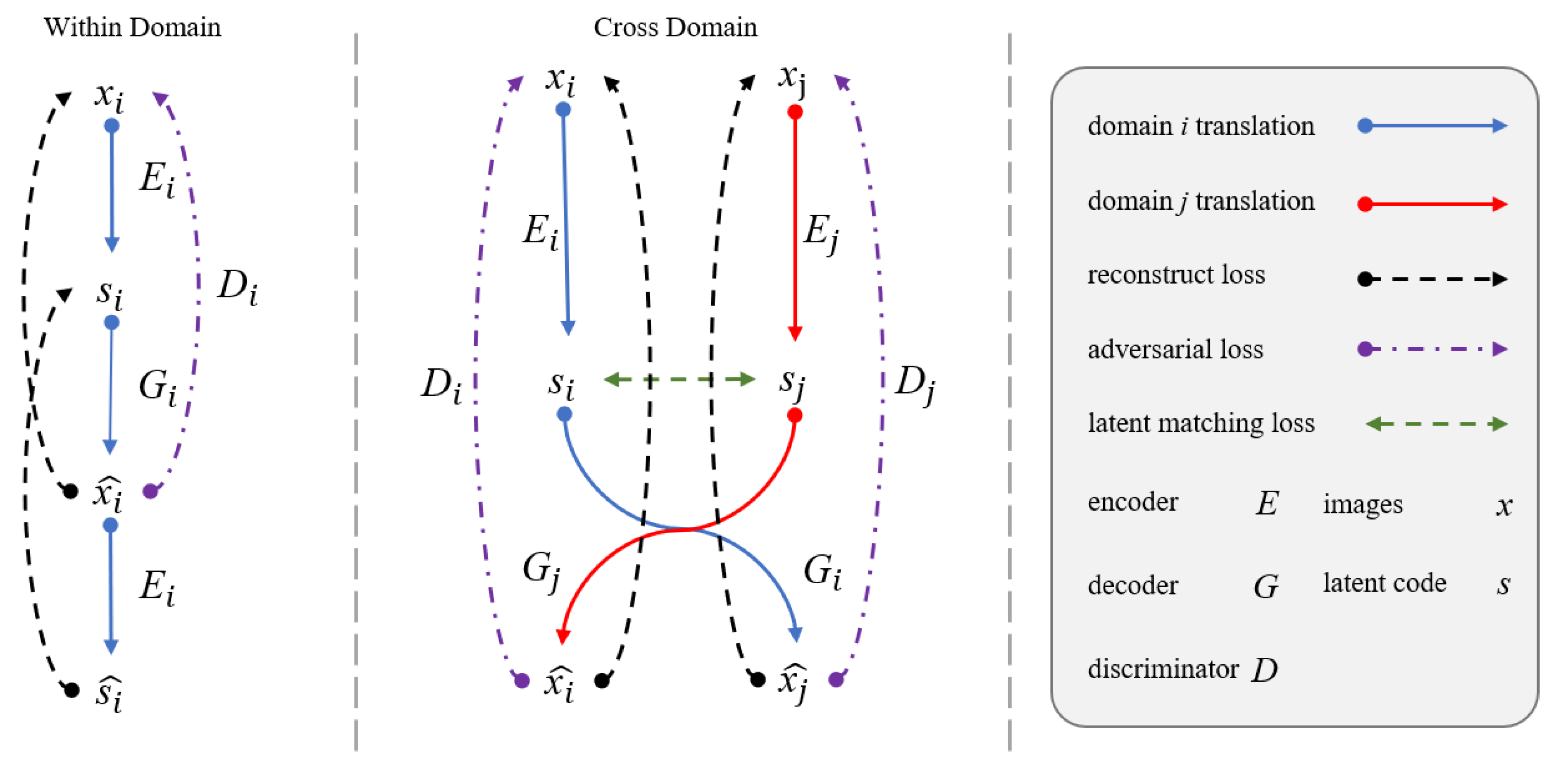
• The introduction of shared latent domain: Through cross domain translation and within domain self-reconstruction training, the shared latent domain fits the joint probability distribution of the multi-spectral domain, and can parse and store diversity and the characteristics of each spectral domain. It is the end of encoders and the beginning of the decoders of all spectral domains. In this way, the parameter expansion problem of many-to-many translation is avoided.
• The introduction of multimodal feature map: By introducing discrete feature (e.g., surface type and cloud map type), and numerical feature maps (e.g., surface temperature), the location accuracy of the surface area is improved, and the limitations of spectral characterization information are overcome.
• The training is conducted on the supervised spatio-temporal matching data sets, combined with cycle consistency loss and perceptual loss, to ensure the uniqueness of the output result and improve spectral translation accuracy.

The structure of this paper is as follows: In Section 2, the structure and loss functions of the GAN used in this study are introduced. In Section 3, the building of the datasets and the experiments to evaluate different methods are elaborated. Finally, future work and conclusions are given in Section 4.

2. Materials and Methods

We begin with an overview of the spectral domain translation method, and then, the basic assumptions and model architectures are introduced. Finally, the loss function of networks and the training process are described.

2.1. Overview of the Method

In this work, a multi-spectral domain translation generation adversarial model is proposed for remote sensing images. Following the basic framework of image-conditional GANs [12], the model has an independent encoder E, a decoder G, and a discriminator D for each spectral domain. The difference is that the model assumes the existence of a shared latent domain, which make it possible to encode each spectral domain into that space and reconstruction of information from that space.

In the training process, the shared latent domain is constructed in two ways. First, the source domain spectral image and the target domain spectral image are encoded to the feature matrix with the same size. The training with L1 loss makes the encoded feature matrix consistent across spectral domains. Second, in within domain training, the source and target domains use their encoders and decoders to achieve image reconstruction from the feature matrix. In cross domain training, the feature matrices output from the source and target domain encoders are exchanged, and then the images are reconstructed following the above steps. The purpose of this step is to enable decoders in different spectral domains to obtain the information needed for their reconstruction from the shared latent domain.

During the test, there is no need to reload all the encoders and decoders. Only the combination of encoders for the source domain spectrum and the combination of decoders for the target domain need to be loaded. The feature matrix is generated by the encoder in the source domain, and then the spectral image is generated by the decoder in the target domain.

Since all encoding and decoding is based on the shared latent domain, the set of spectral domains of the model can be continuously expanded. When a new spectral domain is added, it is only necessary to ensure that the encoder of the new spectral domain can make the image output to the shared latent domain and the decoder can recover its own image from that space.

Meanwhile, the model can add additional physical property information to improve the simulation accuracy. For remote sensing imaging, the underlying surface and clouds are the main influencing factors of optical radiation transfer. Therefore, earth surface classification data $R^{GT}$ and cloud classification data $R^{CLT}$ are used as feature maps to form the boundary conditions of the scene.

2.2. Shared Latent Domain Assumption

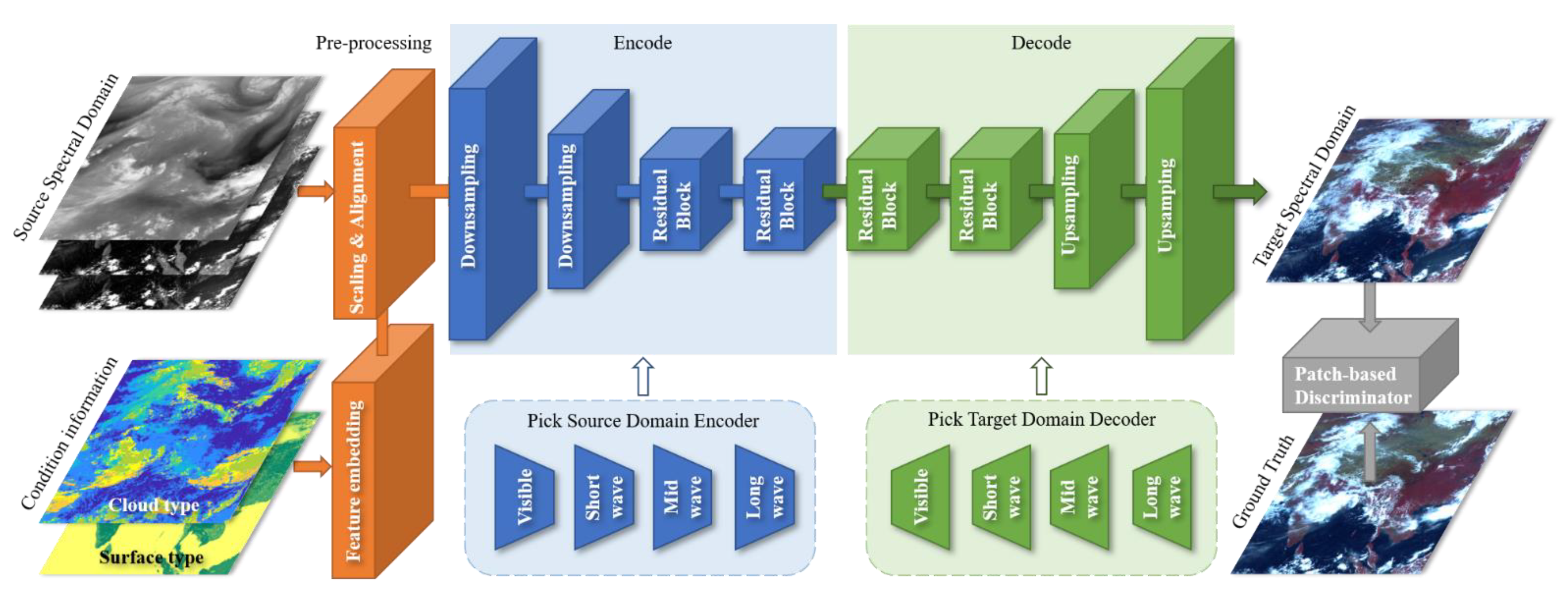
Let $x_i\in {\chi }_i$ be the spectral images from spectral domain ${\chi }_i$, and there are N spectral domains. Let $r\in R$ be the condition information of image boundary condition R. Our goal is to estimate the conditional distribution $p\left(x_i|\left(x_j,r\right)\right)$ between domains i and j with a learned deterministic mapping function $p\left(x_{j\to i}|\left(x_j,r\right)\right)$ and the joint distribution $p\left(x_1,x_2,\cdots ,x_N,r\right)$.

To translate from one spectral domain to multiple spectral domains, this study makes a fully shared latent space assumption [17,29]. It is assumed that each spectral image $x_i$ is generated from a latent code s ∈ S that is shared by all spectral domains and conditional information. Using the shared latent code domain as a bridge, spectral image $x_i$ can be synthesized by decoder $G_i^{*}\left(s\right)$, and the joint probability distribution s can be obtained by encoder $E_i^{*}\left(x_i,r\right)$, so that $E_i^{*}\left(x_i,r\right)={\left(G_i^{*}\left(s\right)\right)}^{-1}=s$.

2.3. Architecture

As shown in Figure 1, the encoder–decoder-discriminator pair constitutes the SDTGAN model. Considering that the intrinsic information of an image is shared among multiple spectral domains, the output matrix dimensions of the encoder of all spectral-domain models are consistent.

In the process of image translation from source spectral domain ${\chi }_i$ to target spectral domain ${\chi }_j$, the source-domain encoder $E_i$ is selected from the encoder library, and the target-domain decoder $G_j$ is selected from the decoder library. The encoder $E_i$ maps the input matrix to the shared latent code s, and the decoder $G_j$ reconstructs the target spectral-domain image from the latent code s. Then, the adversarial loss is calculated by the target-domain discriminator $D_j$. Since the latent code is shared in each spectral domain, the latent code generated by the source spectral-domain encoding can be decoded into multiple codes in the target spectral domain. Meanwhile, the input matrices need to be preprocessed, including the source spectral image matrix and the condition information matrix after feature embedding.

2.3.1. Generative Network

The generative network is based on the architecture proposed by Johnson et al. [30]. The encoder consists of a set of stride-2 downsampling and convolutional layers and several residual blocks. The decoder processes the latent code by a set of residual blocks and then restores the image size through 1/2-strided upsampling and convolutional layers.

2.3.2. Patch Based Discriminator Network

The patch discriminator with different fields of view is used [31,32]. The discriminator outputs a predicted probability value for each area (patch) of the input image. Evolving from judging whether the input is true or false, patch discriminator judges whether the input area with a size of N × N is true or false. The discriminator with a large perceptual field ensures the consistency of geographic location, and discriminator with a small perceptual field ensures the characteristics of texture details.

2.3.3. Feature Embedding

The information carried by spectral images with few bands is limited. For instance, the earth’s surface is seriously obscured in the water vapor bands. In the process of spectrum translation, it is difficult for the model to accurately derive the surface structure. To address this issue, feature maps are added to the input matrix to fill the lack of information in the spectrum.

Remote sensing image features include discrete features and numerical features. The semantic labels of pixels such as land surface type and cloud cover type are discrete features; the quantitative information of pixel areas such as land surface temperature and cloud cover rate are numerical features. For discrete features, this study pre-allocates a fixed number of channels for each category, and encodes the label as a one-hot vector. For numeric features, this study pre-sets the interval of the upper and lower limits of the value, and then normalizes the value to [0, 1]. Then, the size of the feature map is adjusted to that of the spectral image. Finally, the feature matrix and the spectral matrix are combined and input to the encoder.

2.4. Loss Function

Based on the paired dataset, this study introduces the bidirectional reconstruction loss [29] to achieve the reversibility of the encoding and decoding processes and reduce the redundant function mapping space. Meanwhile, this study adopts the objective function to make all encoders output to the same latent space, and the images of various spectral domains can be reconstructed from the latent space. Figure 2 shows the training flow of the loss function for with-domain and cross-domain.

2.4.1. Reconstruction loss

Based on the reversibility of the encoder and decoder, an objective function that enables the cycle consistency of image and feature coding is constructed. The use of cross-domain reconstruction consistency constrains the spatial diversity of the encoding and decoding between multiple domains, and it stabilizes spectral-domain translation results. Previous studies have found adding reconstruction loss with L1 loss is conducive to reducing the probability of model collapse [13,29].

• Within domain reconstruction loss

Given an image sampled from the data distribution, its spectral image and latent code after encoding and decoding can be reconstructed, and the within-domain reconstruction loss can be defined as:

$$L_{\mathrm{Re}con}^{x_i}={\lambda }_{\mathrm{I}}{\mathbb{E}}_{x_i,r\sim p\left(x_i,r\right)}\left[{\Vert G_i\left(E_i\left(x_i,r\right)\right)-x_i\Vert }_1\right]+{\lambda }_{\mathrm{E}}{\mathbb{E}}_{x_i,r\sim p\left(x_i,r\right)}\left[{\Vert E_i\left(G_i\left(E_i\left(x_i,r\right)\right)\right)-E_i\left(x_i,r\right)\Vert }_1\right]$$

(1)

where ${\lambda }_{\mathrm{I}}$ and ${\lambda }_{\mathrm{E}}$ are the weights that control the importance of image reconstruction term and latent code reconstruction term, respectively.

2.

Cross domain reconstruction loss

Given two spectra domain images sampled from the joint data distribution, their spectral images after exchanging encoding and decoding can be reconstructed, and its cross domain reconstruction loss can be defined as:

$$L_{\mathrm{Re}con}^{x_i,x_j}={\mathbb{E}}_{x_i,x_j,r\sim p\left(x_i,x_j,r\right)}\left[{\Vert G_i\left(E_j\left(x_j,r\right)\right)-x_i\Vert }_1\right]+{\mathbb{E}}_{x_i,x_j,r\sim p\left(x_i,x_j,r\right)}\left[{\Vert G_j\left(E_i\left(x_i,r\right)\right)-x_j\Vert }_1\right]$$

(2)

$$L_{\mathrm{Recon}}={\lambda }_{\mathrm{within}}{\displaystyle \sum _{i=1}^N{L}_{\mathrm{Re}con}^{x_i}}+{\lambda }_{\mathrm{cross}}{\displaystyle \sum _{i=1}^N{\displaystyle \sum _{j=i+1}^N{L}_{\mathrm{Re}con}^{x_i,x_j}}}$$

(3)

where $L_{\mathrm{Recon}}$ is the sum of the multi-domain reconstruction loss; ${\lambda }_{\mathrm{within}}$ and ${\lambda }_{\mathrm{cross}}$ are weights that control the importance of the within-domain reconstruction term and cross-domain reconstruction term, respectively.

2.4.2. Latent Matching loss

Given two multi-spectral images sampled from the same data distribution, the latent code should be matched after encoding. In previous work, auto-encoders and GANs use KLD loss, and adversarial loss [16,33] or implicitly constrain [29] the latent domain distribution. The present model uses the calculation of L1 Loss across domains to strongly constrain different domains to encode in the same space.

$$L_{LM}^{x_i,x_j}={\mathbb{E}}_{x_i,x_j,r\sim p\left(x_i,x_j,r\right)}\left[{\Vert E_i\left(x_i,r\right)-E_j\left(x_j,r\right)\Vert }_1\right]$$

(4)

$$L_{\mathrm{Match}}={\displaystyle \sum _{i=1}^N{\displaystyle \sum _{j=i+1}^N{L}_{LM}^{x_i,x_j}}}$$

(5)

where $L_{LM}^{x_i,x_j}$ is the latent matching loss that depicts the L1 loss between the latent of the i-domain and j-domain images under the joint probability distribution.

2.4.3. Adversarial loss

This study employs Patch-GANs to distinguish between the real images or the images translated from the latent space in the target domain.

$$\begin{array}{l}{L}_{\mathrm{GAN}}^{x_i}={\mathbb{E}}_{x_i,r\sim p\left(x_i,r\right)}\left[\log \left(1-D_i\left(G_i\left(E_i\left(x_i,r\right)\right)\right)\right)\right]\\ \begin{array}{ccc}& & +\end{array}{\mathbb{E}}_{x_i,r\sim p\left(x_i,r\right)}\left[\log \left(D_i\left(x_i\right)\right)\right]\end{array}$$

(6)

$$L_{\mathrm{GAN}}^{x_{j\to i}}={\mathbb{E}}_{x_i,x_j,r\sim p\left(x_i,x_j,r\right)}\left[\log \left(1-D_i\left(G_i\left(E_j\left(x_j,r\right)\right)\right)\right)\right]$$

(7)

$$L_{\mathrm{GAN}}={\lambda }_{\mathrm{cross}}{\displaystyle \sum _{i=1}^N{\displaystyle \sum _{j=i+1}^N{L}_{\mathrm{GAN}}^{x_{j\to i}}}+}{\lambda }_{\mathrm{within}}{\displaystyle \sum _{i=1}^N{L}_{\mathrm{GAN}}^{x_i}}$$

(8)

where $L_{\mathrm{GAN}}^{x_i}$ is the within-domain GAN loss of the images sampled from domain i; $L_{\mathrm{GAN}}^{x_{j\to i}}$ is the cross-domain GAN loss that depicts the GAN loss of spectral image translation from domain j to domain i, and $L_{GAN}$ is the sum of multi-domain GAN loss.

2.4.4. Total Loss

In this study, the model is optimized through joint training of encoders, decoders, and discriminators in all spectral domains. The total loss function is the weighted sum of the counter loss, reconstruction loss, and latent matching loss in each spectral domain.

When a new spectral domain is added to the trained multi-spectral domain model, the model parameters of the existing spectral domain can be fixed, and the shared feature space can be exploited to accelerate the training process and avoid the expansion of training parameters.

$$\underset{E,G}{\min }\underset{D}{\max }{L}_{\mathrm{Total}}\left(E,G,D\right)={\lambda }_{\mathrm{GAN}}{L}_{\mathrm{GAN}}+{\lambda }_{\mathrm{Recon}}{L}_{\mathrm{Re}con}+{\lambda }_{\mathrm{Match}}{L}_{\mathrm{Match}}$$

(9)

where ${\lambda }_{\mathrm{GAN}}$, ${\lambda }_{\mathrm{Recon}}$, and ${\lambda }_{\mathrm{Match}}$ are weights that control the importance of loss terms.

2.5. Traning Process

In the initial training of the model, all source and target domains are combined into a set that contains N spectral domains. Then, the SDTGAN model is trained by updating the generators and discriminators alternately, which follows the basic rule of GANs. The training of generators is the key point of the method, and the steps are illustrated in the following Algorithm 1.

Algorithm 1. Generators training process in a single iteration

for i = 1 to N

for j = i + 1 to N

$L_{\mathrm{Re}con}^{x_i}\leftarrow {\Vert G_i\left(E_i\left(x_i,r\right)\right)-x_i\Vert }_1$

$L_{\mathrm{Re}con}^{x_j}\leftarrow {\Vert G_j\left(E_j\left(x_j,r\right)\right)-x_j\Vert }_1$

$L_{\mathrm{Re}con}^{x_i,x_j}\leftarrow {\Vert G_j\left(E_i\left(x_i,r\right)\right)-x_j\Vert }_{1}and{\Vert G_i\left(E_j\left(x_j,r\right)\right)-x_{is}\Vert }_1$

$L_{LM}^{x_i,x_j}\leftarrow {\Vert E_i\left(x_i,r\right)-E_j\left(x_j,r\right)\Vert }_1$

$L_{\mathrm{GAN}}^{x_i}\leftarrow D_i\left(G_i\left(E_i\left(x_i,r\right)\right)\right)$

$L_{\mathrm{GAN}}^{x_j}\leftarrow D_j\left(G_j\left(E_j\left(x_j,r\right)\right)\right)$

$L_{\mathrm{GAN}}^{x_{i\to j}}\leftarrow D_j\left(G_j\left(E_i\left(x_i,r\right)\right)\right)$

$L_{\mathrm{GAN}}^{x_{j\to i}}\leftarrow D_i\left(G_i\left(E_j\left(x_j,r\right)\right)\right)$

$L_{\mathrm{Total}}$ update

Backward gradient decent

Optimizer update

end for

end for

3. Experiment

3.1. Datasets

In the experiment, the paired data consists of spectral remote sensing images of earth background and condition information data including earth surface type data and cloud type data. For paired data of spectral images, the earth coordinates corresponding to each pixel need to be aligned since the task aims to achieve spectral translation at the pixel level of the image. The model establishes the mapping relationship between spectra by learning the intensity mapping relationship originating from the same location and time of the sampled images.

3.1.1. Remote sensing Datasets

This study takes the L1 level data obtained by the multi-channel scanning imaging radiometer of the FY-4A satellite [34,35] as the satellite spectral image data. The FY-4A satellite is a new generation of China’s geostationary meteorological satellite, and it is equipped with various observation instruments including the Advanced Geosynchronous Radiation Imager (AGRI). As shown in

Table 1. The description of spectral image information.

Channel ID	Description	Band (μm)	Spatial Resolution (km)	Main Application
CH01	Visible & Near-Infrared	0.45~0.49	1	Aerosol
CH02		0.55~0.75	0.5~1	Fog, Cloud
CH03		0.75~0.90	1	Vegetation
CH04	Short-Wave Infrared	1.36~1.39	2	Cirrus
CH05		1.58~1.64	2	Cloud, Snow
CH06		2.1~2.35	2~4	Cirrus, Aerosol
CH07	Mid-Wave Infrared	3.5~4.0 (High)	2	Fire
CH08		3.5~4.0 (Low)	4	Land Surface
CH09	Water Vapor	5.8~6.7	4	Water Vapor
CH10		6.9~7.3	4	Water Vapor
CH11	Long-Wave Infrared	8.0~9.0	4	Water Vapor,
CH12		10.3~11.3	4	Cloud
CH13		11.5~12.5	4	Surface Temperature
CH14		13.2~13.8	4	Surface Temperature

, AGRI has 14 spectral bands from visible to infrared (0.45–13.8 μm) with a high spatial resolution (1 km for visible light channels, 2 km for near-infrared channels, and 4 km for remaining infrared channels) and temporal resolution (full-disk images at the 15-min interval).

The daily data from January to December 2020 were used for the training process, and the daily data from June to August 2020 were used for testing. The daily data are sampled from 12:00 in the satellite’s time zone, to maximize the visible area in the image.

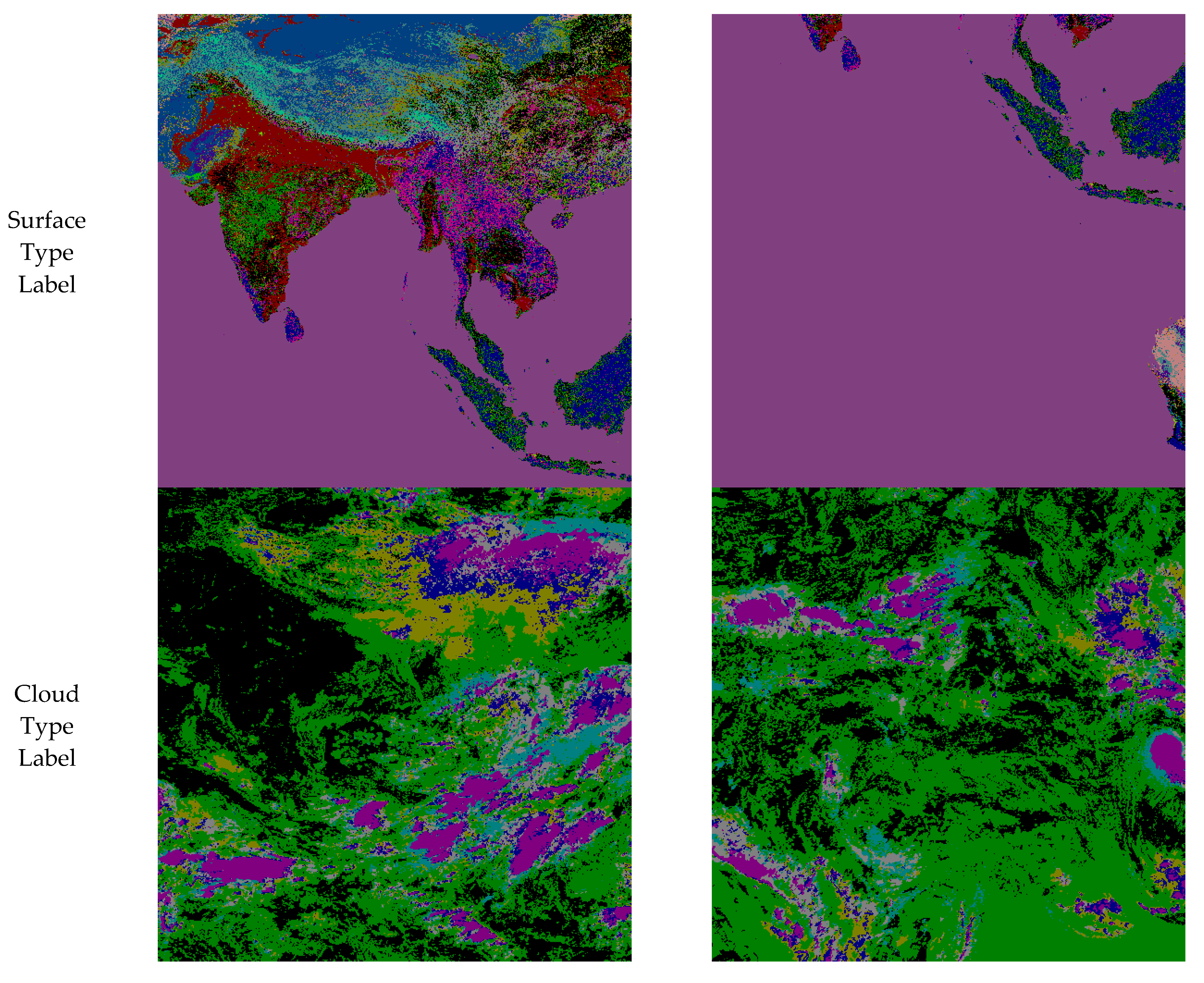
3.1.2. Condition Information Dataset

(1)

Earth surface type

The earth surface type data is obtained from the global land cover maps (GlobCover [36]) developed and demonstrated by ESA. The theme legend of GlobCover is compatible with that of the UN Land Cover Classification System (LCCS).

As shown in

Table 2. The description of the earth surface type label.

Label	Type
0	Post-flooding or irrigated croplands
1	Rainfed croplands
2	Mosaic Cropland (50–70%)/Vegetation (grassland, shrubland, forest) (20–50%)
3	Mosaic Vegetation (grassland, shrubland, forest) (50–70%)/Cropland
4	Closed to open (>15%) broadleaved evergreen and/or semi-deciduous forest (>5 m)
5	Closed (>40%) broad leaved deciduous forest (>5 m)
6	Open (15–40%) broad leaved deciduous forest (>5 m)
7	Closed (>40%) needle leaved evergreen forest (>5 m)
8	Open (15–40%) needle leaved deciduous or evergreen forest (>5 m)
9	Closed to open (>15%) mixed broadleaved and needle leaved forest (>5 m)
10	Mosaic Forest/Shrubland (50–70%)/Grassland (20–50%)
11	Mosaic Grassland (50–70%)/Forest/Shrubland (20–50%)
12	Closed to open (>15%) shrubland (<5 m)
13	Closed to open (>15%) grassland
14	Sparse (>15%) vegetation (woody vegetation, shrubs, grassland)
15	Closed (>40%) broadleaved forest regularly flooded-Fresh water
16	Closed (>40%) broadleaved semi-deciduous and/or evergreen forest regularly flooded-Saline water
17	Closed to open (>15%) vegetation (grassland, shrubland, woody vegetation) on regularly flooded or waterlogged soil-Fresh, brackish or saline water
18	Artificial surfaces and associated areas (urban areas >50%)
19	Bare areas
20	Water bodies
21	Permanent snow and ice
22	No data

, GlobCover is a static global gridded surface type map with a resolution of 300 m and 23 classification types. Since the surface type labels of GlobCover are encoded as one-hot vectors, they are rearranged in this study.

(2)

Cloud type

The cloud classification data is obtained from the L2 level real-time product of the FY4A satellite. According to the microphysical structure and thermodynamic properties of the cloud, the effective absorption optical thickness ratios of the four visible light channels have different properties. As shown in

Table 3. The description of the cloud type label.

Label	Type
0	Clear
1	Water Type
2	Super Cooled Type
3	Mixed Type
4	Ice Type
5	Cirrus Type
6	Overlap Type
7	Uncertain
8	Space
9	Fill Number

, there are 10 categories of cloud type labels included in the image. The sampling moment for cloud classification is the same as that of spectral images, thus forming paired data.

3.2. Implementation Details

In the experiment, the parameters of the proposed method were fixed. For the network architecture, each encoder contains three convolutional layers for downsampling and three residual blocks for feature extraction. The decoder adopts the symmetric structure of the encoder, including three layers of residual blocks and three layers of upsampling convolutional layers. The discriminators consist of stacks of convolutional layers. Besides, LeakyReLU was used for nonlinearity. The hyper-parameters were set as follows:

$${\lambda }_{\mathrm{I}}=1,{\lambda }_E=1,{\lambda }_{\mathrm{within}}=1,{\lambda }_{\mathrm{cross}}=10,{\lambda }_{\mathrm{GAN}}=1,{\lambda }_{\mathrm{Recon}}=1\mathrm{and}{\lambda }_{\mathrm{Match}}=1.$$

The translation models taken for comparison include the SDTGAN model using surface type tags, the SDTGAN model using both surface type tags and cloud type tags, the pix2pixHD model, the cycleGAN model, and the UNIT model. Among these models, SDTGAN, cycleGAN, and UNIT can achieve multiple outputs for a single model, and pix2pixHD needs to exchange input and output data to train two sets of models.

For all models, the training was repeated for 200 epochs on an NVIDIA RTX3090 GPU with 24GB GPU memory. The weights were initialized with Kaiming initialization [37]. The Adam optimizer [38] was used, and the momentum was set to 0.5. The learning rate was set to 0.0001, and it linearly decayed after 100 epochs. Instance normalization [39] was used, which is more suitable for scenes with high requirements for a single pixel was used. Reflection padding was used to reduce artifacts. The size of the input and output image blocks for training was 512 × 512. Each mini-batch consisted of one image from each domain.

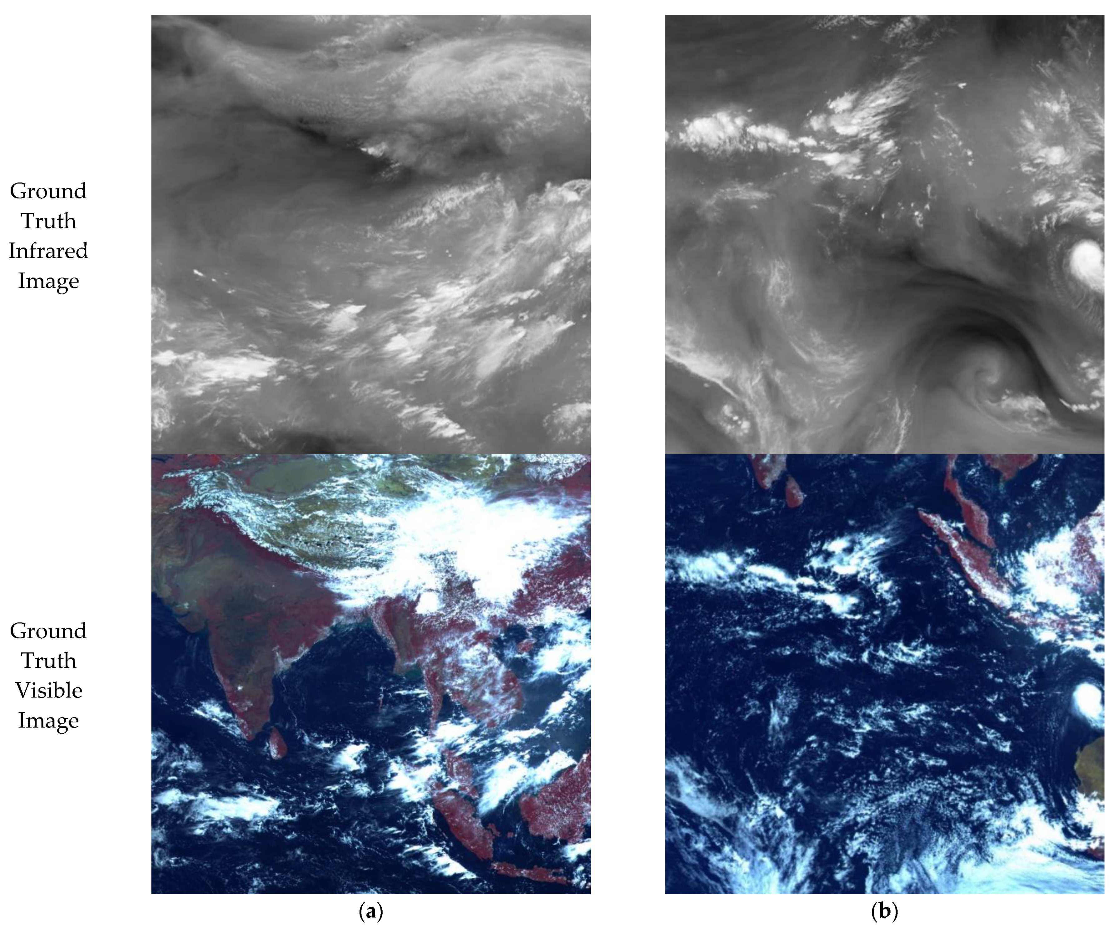
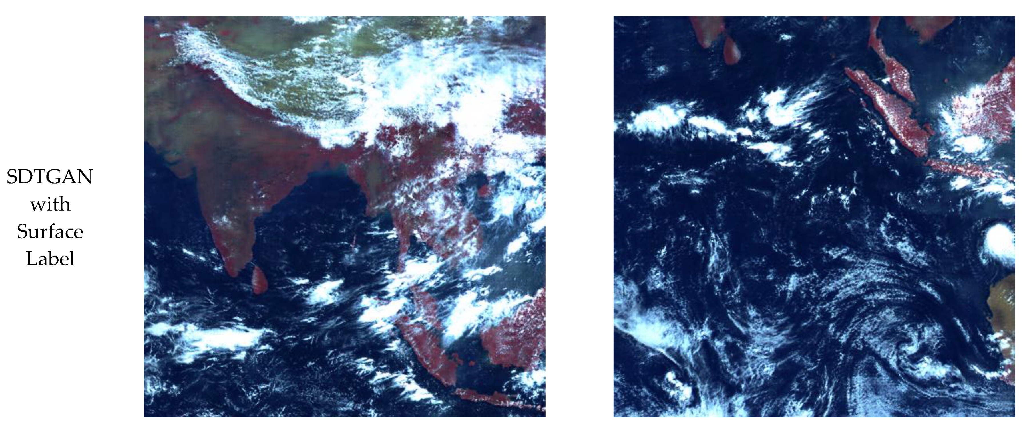
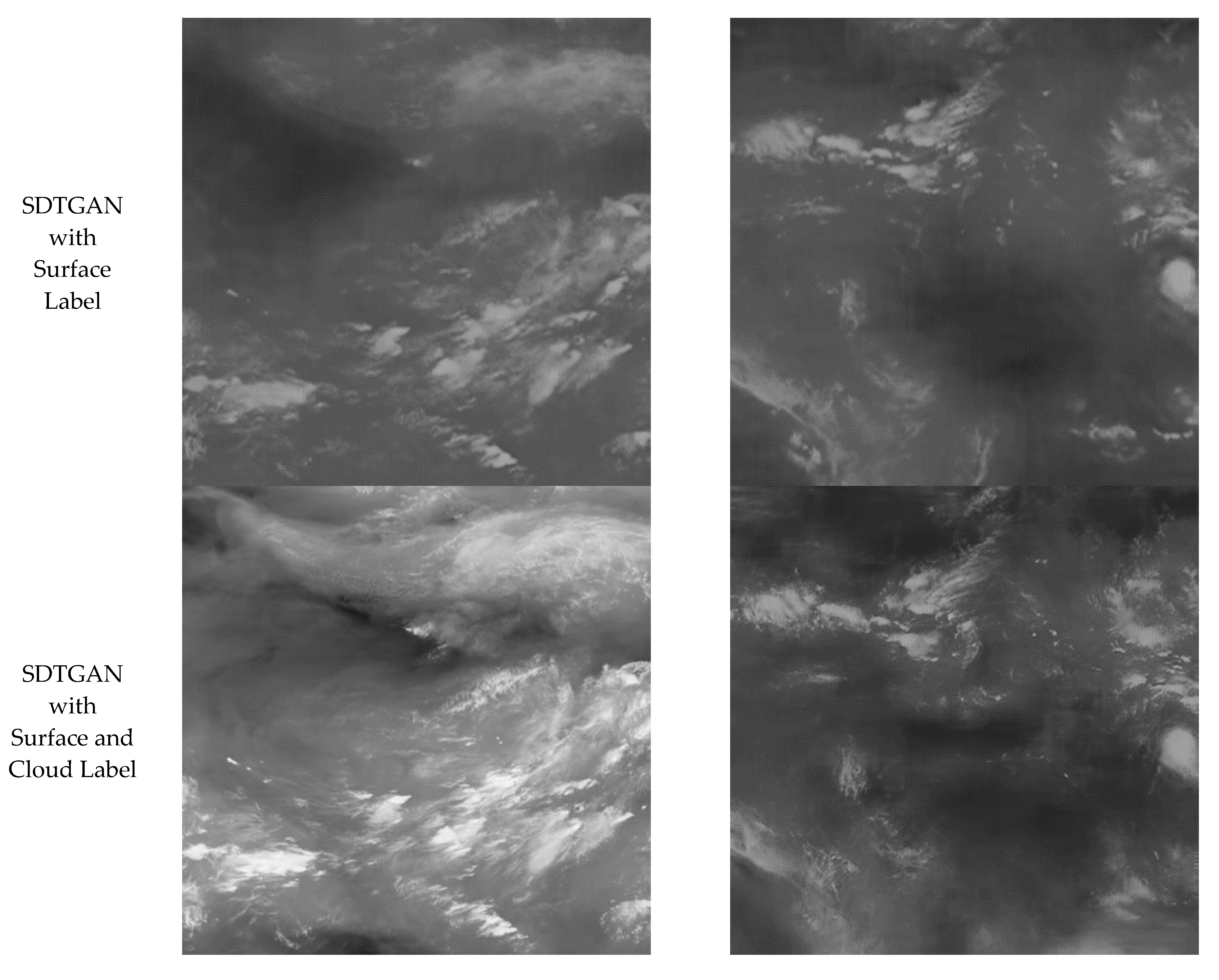
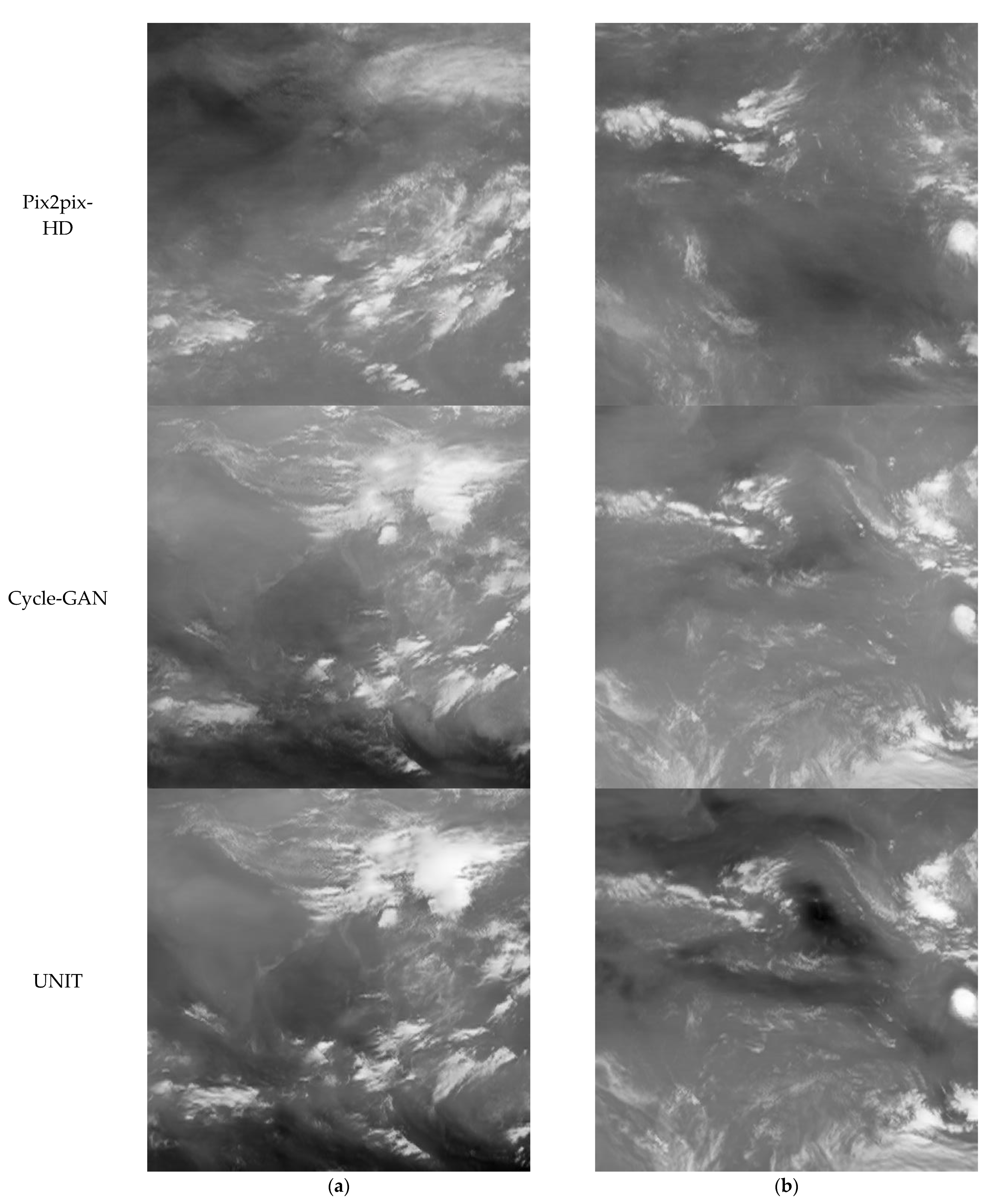
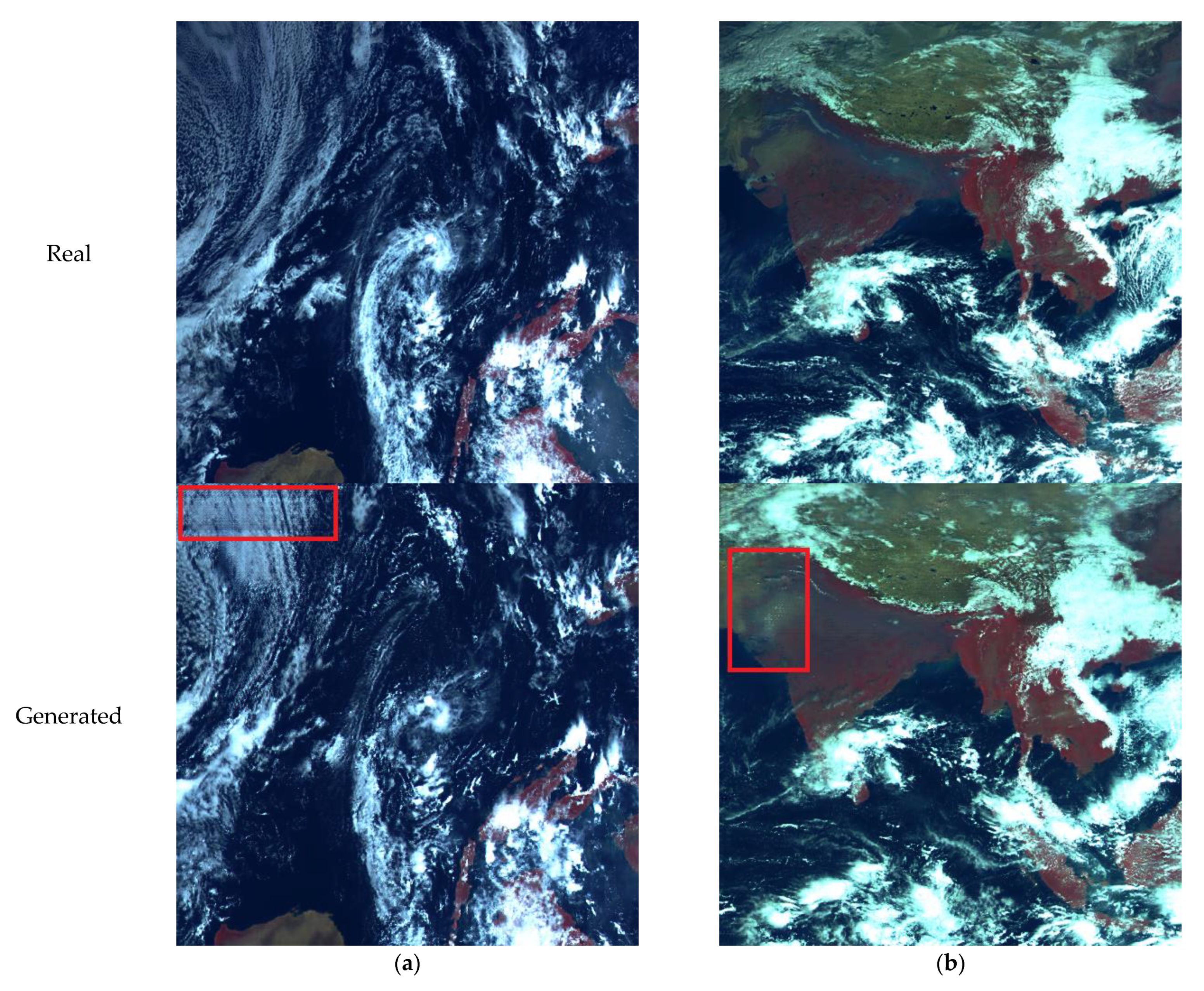
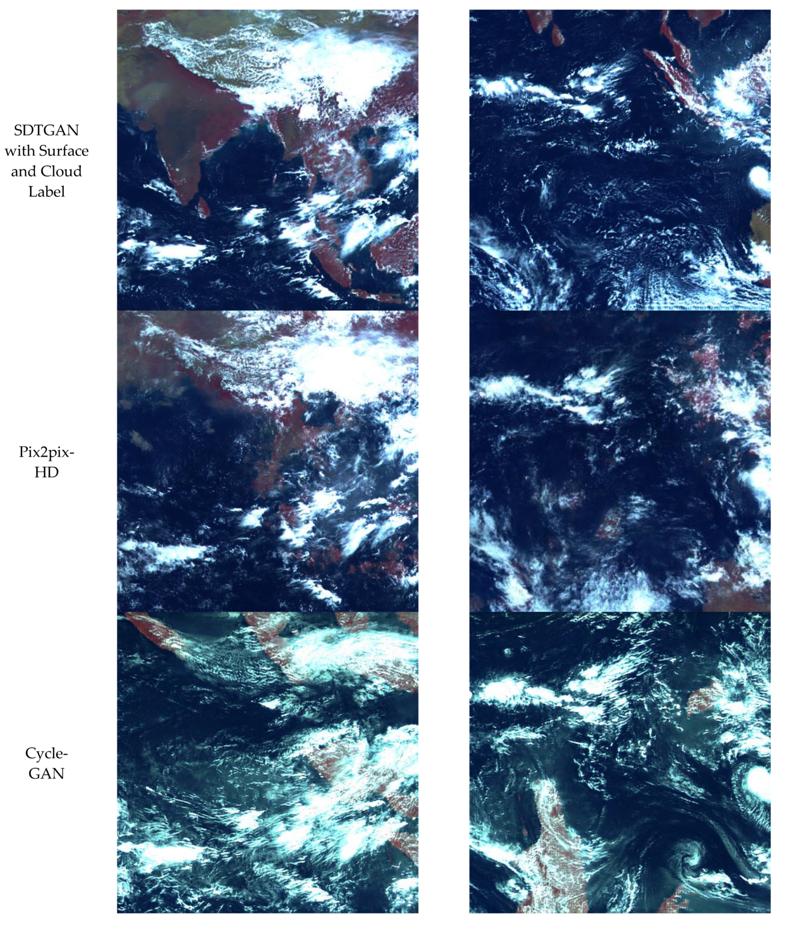
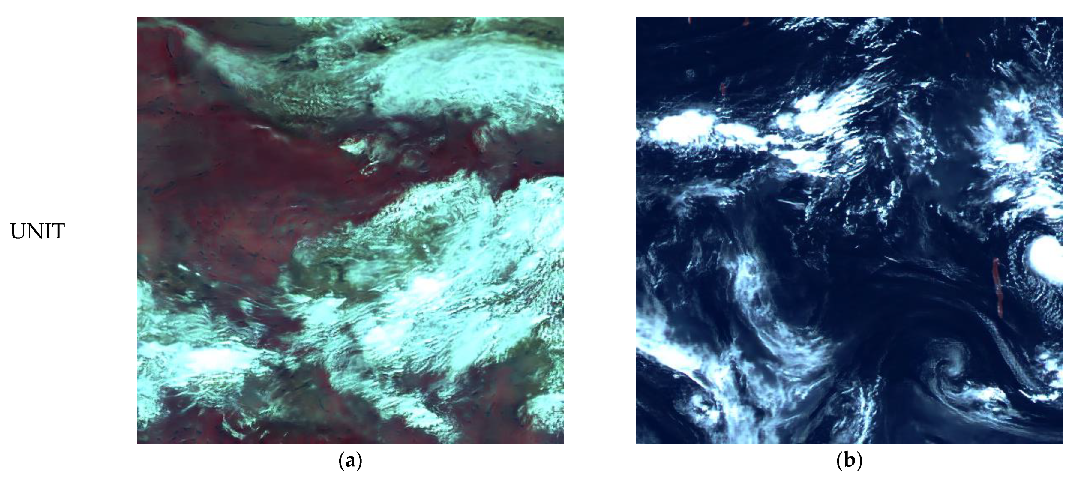
3.3. Visual Comparison

In this work, the first three reflection channels of AGRI (CH01, CH02, and CH03) are used for visible light spectrum combination. The combined images of the three RGB channels are more in line with the human eye observation and can effectively visualize the details of oceans, lands, and clouds. Meanwhile, the long-wave infrared band CH11 is used, and its main visual content is water vapor and cloud features. Due to the lack of features of the underlying surface of the earth in the visual results of CH11, the image translation from the infrared spectral domain to the visible spectral domain poses a challenge to the model.

Figure 3, Figure 4 and Figure 5 illustrate two examples of the translation between the above two sets of spectral remote sensing images. Each set contains image information such as oceans, lands, and clouds. In Figure 3, the underlying surface of the earth in group (a) is mainly land, and that of the earth in group (b) is dominated by the ocean. Figure 4 shows the visual comparison of different models for translation from infrared spectrum domain to visible spectrum domain. Figure 5 shows the visual comparison of different models for translation from visible spectrum domain to infrared spectrum domain.

3.4. Digital Comparison

To quantitatively measure the proposed method, three image quality metrics, i.e., mean-square-error (MSE), peak signal-to-noise ratio (PSNR), and structural similarity index (SSIM) [40], are selected to evaluate the translation effectiveness. MSE measures the difference between the real and simulated values. The smaller the MSE is, the more similar the two images are. PSNR is a traditional image quality evaluation index. A higher PSNR generally indicates a higher image quality. SSIM measures the structural similarity between the real image and the simulated image.

The test dataset used in the visual comparison is also taken for quantitative comparison. The dataset includes 500 remote sensing images. The average values of the evaluation metrics are calculated, and the results are listed in

Table 4. Quality result of the translation from infrared spectrum domain to visible spectrum domain.

Method	MSE	PSNR	SSIM
CycleGAN	0.0979	10.1333	0.347
UNIT	0.0931	10.3951	0.3841
Pix2pixHD	0.0663	11.8969	0.4846
SDTGAN with Surface Label	0.0361	14.5794	0.6246
SDTGAN with Surface and Cloud Label	0.0237	16.4055	0.7018

and

Table 5. Quality result of the translation from visible spectrum domain to infrared spectrum domain.

Method	MSE	PSNR	SSIM
CycleGAN	0.0521	13.014	0.7148
UNIT	0.1592	8.1298	0.5055
Pix2pixHD	0.0105	19.9687	0.775
SDTGAN with Surface Label	0.0017	27.9227	0.8695
SDTGAN with Surface and Cloud Label	0.0019	27.6883	0.9031

, where optimal values are highlighted in bold.

The results of Table 4 and Table 5 show that the proposed SDTGAN method is superior to other comparative methods. It achieves better image recognizable structure and data authenticity in the spectral domain translation from infrared spectrum domain to visible spectrum domain and vice versa.

3.5. Ablation Study

The against ablations of within domain reconstruction loss, cross domain reconstruction loss, and latent matching loss are compared. In this case, the basic model contains only adversarial loss. As shown in

Table 6. Ablation study of the translation from infrared spectrum domain to visible spectrum domain.

Method	MSE	PSNR	SSIM
Basic	0.0393	14.1868	0.5986
Basic + within Domain Reconstruction Loss	0.0382	14.2955	0.5867
Basic + cross Domain Reconstruction Loss	0.0251	16.0984	0.6801
Basic + Latent Matching Loss	0.0326	14.9459	0.6195

and

Table 7. Ablation study of the translation from visible spectrum domain to infrared spectrum domain.

Method	MSE	PSNR	SSIM
Basic	0.0037	24.4947	0.5256
Basic + within Domain Reconstruction Loss	0.0048	23.3879	0.8383
Basic + cross Domain Reconstruction Loss	0.0019	27.6244	0.898
Basic + Latent Matching Loss	0.0032	25.083	0.56

, adding reconstruction loss and latent matching loss alone can effectively improve the evaluation metrics of the images, and the model including all the loss functions achieves the highest evaluation score.

3.6. Limitation

The spectral translation task involves the transformation of energy intensity and graphic texture. In most cases, the model can generate plausible cloud and continental shapes. However, there are still many cases in which the model causes loss of details and distortions. As shown in Figure 6a, in the real image, the ocean is covered with large areas of thin clouds, yet. The generated image has difficulty in inferring the random phenomenal changes over a large area, thus yielding an erroneous result. As shown in Figure 6b, in continental terrain, a certain distortion and blurring is produced for the boundary areas with variable shapes.

These detail distortions may be due to the limitations in the structure of the generative network or feature selection. In future work, we will continue to explore these issues. For example, by selecting the feature data that can represent cloud height, and surface temperature, and enhancing the generated details of textures by better network structures.

4. Conclusions and Future Work

In this paper, a multi-spectral domain translation model based on conditional GAN architecture is proposed for remote sensing images of the earth background. To achieve multi-spectral domain adaptation, the model introduces feature maps of earth background and shared latent domain. In addition to adversarial loss, within domain reconstruction loss, cross domain reconstruction loss and latent matching loss are added to train the network. Besides, multi-spectral remote sensing images taken from a FY satellite are used as a dataset to test the effect of bidirectional translation between infrared band and visible band images. Compared with models such as pix2pix and cycleGAN, SDTGAN achieves more stable and accurate performance in translating spectral images at the pixel level, and simulating the surface structure and texture of clouds. In future work, we will explore a better structure for extraction, construction, and utilization of shared latent domain for spectral-domain translation, and extend it to other band combinations.

References

1. Srivastava, A.; Oza, N.; Stroeve, J. Virtual sensors: Using data mining techniques to efficiently estimate remote sensing spectra. IEEE Trans. Geosci. Remote Sens. 2005, 43, 590–600. [Google Scholar] [CrossRef]
2. Miller, S.W.; Bergen, W.R.; Huang, H.; Bloom, H.J. End-to-end simulation for support of remote sensing systems design. Proc. SPIE-Int. Soc. Opt. Eng. 2004, 5548, 380–390. [Google Scholar]
3. Börner, A.; Wiest, L.; Keller, P.; Reulke, R.; Richter, R.; Schaepman, M.; Schläpfer, D. SENSOR: A tool for the simulation of hyperspectral remote sensing systems. ISPRS J. Photogramm. Remote Sens. 2001, 55, 299–312. [Google Scholar] [CrossRef]
4. Gastellu-Etchegorry, J.P.; Martin, E.; Gascon, F. DART: A 3D model for simulating satellite images and studying surface radiation budget. Int. J. Remote Sens. 2004, 25, 73–96. [Google Scholar] [CrossRef]
5. Gascon, F.; Gastellu-Etchegorry, J.P.; Lefevre, M.-J. Radiative transfer model for simulating high-resolution satellite images. IEEE Trans. Geosci. Remote Sens. 2001, 39, 1922–1926. [Google Scholar] [CrossRef]
6. Ambeau, B.L.; Gerace, A.D.; Montanaro, M.; McCorkel, J. The characterization of a DIRSIG simulation environment to support the inter-calibration of spaceborne sensors. In Proceedings of the Earth Observing Systems XXI, San Diego, CA, USA, 19 September 2016; p. 99720M. [Google Scholar]
7. Tiwari, V.; Kumar, V.; Pandey, K.; Ranade, R.; Agrawal, S. Simulation of the hyperspectral data using Multispectral data. In Proceedings of the 2016 IEEE International Geoscience and Remote Sensing Symposium (IGARSS), Beijing, China, 10–15 July 2016; pp. 6157–6160. [Google Scholar]
8. Rengarajan, R.; Goodenough, A.A.; Schott, J.R. Simulating the directional, spectral and textural properties of a large-scale scene at high resolution using a MODIS BRDF product. In Proceedings of the Sensors, Systems, and Next-Generation Satellites XX, Edinburgh, UK, 19 October 2016; p. 100000Y. [Google Scholar]
9. Cheng, X.; Shen, Z.-F.; Luo, J.-C.; Shen, J.-X.; Hu, X.-D.; Zhu, C.-M. Method on simulating remote sensing image band by using groundobject spectral features study. J. Infrared Millim. WAVES 2010, 29, 45–48. [Google Scholar] [CrossRef]
10. Geng, Y.; Mei, S.; Tian, J.; Zhang, Y.; Du, Q. Spatial Constrained Hyperspectral Reconstruction from RGB Inputs Using Dictionary Representation. In Proceedings of the IGARSS 2019 IEEE International Geoscience and Remote Sensing Symposium, Yokohama, Japan, 28 July–2 August 2019; pp. 3169–3172. [Google Scholar]
11. Han, X.; Yu, J.; Luo, J.; Sun, W. Reconstruction from Multispectral to Hyperspectral Image Using Spectral Library-Based Dictionary Learning. IEEE Trans. Geosci. Remote Sens. 2018, 57, 1325–1335. [Google Scholar] [CrossRef]
12. Goodfellow, I.; Pouget-Abadie, J.; Mirza, M.; Xu, B.; Warde-Farley, D.; Ozair, S.; Courville, A.; Bengio, Y. Generative Adversarial Nets; MIT Press: Cambridge, MA, USA, 2014. [Google Scholar]
13. Isola, P.; Zhu, J.-Y.; Zhou, T.; Efros, A.A. Image-to-Image Translation with Conditional Adversarial Networks. In Proceedings of the 2017 IEEE Conference on Computer Vision and Pattern Recognition (CVPR), Honolulu, HI, USA, 21–26 July 2017; pp. 5967–5976. [Google Scholar] [CrossRef] [Green Version]
14. Wang, T.-C.; Liu, M.-Y.; Zhu, J.-Y.; Tao, A.; Kautz, J.; Catanzaro, B. High-Resolution Image Synthesis and Semantic Manipulation with Conditional GANs. In Proceedings of the IEEE Conference on Computer Vision and Pattern Recognition, Salt Lake City, UT, USA, 18–23 June 2018; pp. 8798–8807. [Google Scholar]
15. Xiong, F.; Wang, Q.; Gao, Q. Consistent Embedded GAN for Image-to-Image Translation. IEEE Access 2019, 7, 126651–126661. [Google Scholar] [CrossRef]
16. Yi, Z.; Zhang, H.; Tan, P.; Gong, M. Dualgan: Unsupervised dual learning for image-to-image translation. In Proceedings of the IEEE International Conference on Computer Vision, Cambridge, MA, USA, 20–23 June 2017; pp. 2849–2857. [Google Scholar]
17. Zhu, J.-Y.; Park, T.; Isola, P.; Efros, A.A. Unpaired image-to-image translation using cycle-consistent adversarial networks. In Proceedings of the IEEE International Conference on Computer Vision, Venice, Italy, 22–29 October 2017; pp. 2223–2232. [Google Scholar]
18. Hoffman, J.; Tzeng, E.; Park, T.; Zhu, J.-Y.; Isola, P.; Saenko, K.; Efros, A.A.; Darrell, T. CyCADA: Cycle-Consistent Adversarial Domain Adaptation. In Proceedings of the ICML, Stockholm, Sweden, 10–15 July 2018. [Google Scholar]
19. Chen, S.; Liao, D.; Qian, Y. Spectral Image Visualization Using Generative Adversarial Networks. In Proceedings of the Swarm, Evolutionary, and Memetic Computing; Springer Science and Business Media LLC: Secaucus, NJ, USA, 2018; pp. 388–401. [Google Scholar]
20. Shi, Z.; Chen, C.; Xiong, Z.; Liu, D.; Wu, F. HSCNN+: Advanced CNN-Based Hyperspectral Recovery from RGB Images. In Proceedings of the IEEE Conference on Computer Vision and Pattern Recognition (CVPR) Workshops, Salt Lake City, UT, USA, 18–22 June 2018; pp. 939–947. [Google Scholar] [CrossRef]
21. Wu, J.; Aeschbacher, J.; Timofte, R. In Defense of Shallow Learned Spectral Reconstruction from RGB Images. In Proceedings of the 2017 IEEE International Conference on Computer Vision Workshops (ICCVW), Venice, Italy, 22–29 October 2017; pp. 471–479. [Google Scholar]
22. Zhao, Y.; Fu, G.; Wang, H.; Zhang, S. The Fusion of Unmatched Infrared and Visible Images Based on Generative Adversarial Networks. Math. Probl. Eng. 2020, 2020, 1–12. [Google Scholar] [CrossRef]
23. Ma, J.; Ma, Y.; Li, C. Infrared and visible image fusion methods and applications: A survey. Inf. Fusion 2019, 45, 153–178. [Google Scholar] [CrossRef]
24. Tang, R.; Liu, H.; Wei, J. Visualizing Near Infrared Hyperspectral Images with Generative Adversarial Networks. Remote Sens. 2020, 12, 3848. [Google Scholar] [CrossRef]
25. Cheng, W. Creating synthetic meteorology satellite visible light images during night based on GAN method. arXiv 2021, arXiv:2108.04330. [Google Scholar]
26. Ma, J.; Yu, W.; Liang, P.; Li, C.; Jiang, J. FusionGAN: A generative adversarial network for infrared and visible image fusion. Inf. Fusion 2019, 48, 11–26. [Google Scholar] [CrossRef]
27. Arad, B.; Ben-Shahar, O. Sparse Recovery of Hyperspectral Signal from Natural RGB Images. In Proceedings of the European Conference on Computer Vision, Amsterdam, The Netherlands, 11–14 October 2016; pp. 11–14. [Google Scholar]
28. Liu, P.; Zhao, H. Adversarial Networks for Scale Feature-Attention Spectral Image Reconstruction from a Single RGB. Sensors 2020, 20, 2426. [Google Scholar] [CrossRef] [PubMed]
29. Huang, X.; Liu, M.-Y.; Belongie, S.; Kautz, J. Multimodal Unsupervised Image-to-Image Translation; Springer Science and Business Media LLC: Secaucus, NJ, USA, 2018; pp. 179–196. [Google Scholar]
30. Johnson, J.; Alahi, A.; Fei-Fei, L. Perceptual losses for real-time style transfer and super-resolution. In Proceedings of the European Conference on Computer Vision, Amsterdam, The Netherland, 8–16 October 2016; Springer: Berlin/Heidelberg, Germany, 2016; pp. 694–711. [Google Scholar]
31. Shelhamer, E.; Long, J.; Darrell, T. Fully Convolutional Networks for Semantic Segmentation. Available online: https://arxiv.org/abs/1605.06211 (accessed on 1 March 2022).
32. Durugkar, I.; Gemp, I.M.; Mahadevan, S. Generative Multi-Adversarial Networks. arXiv 2017, arXiv:1611.01673. [Google Scholar]
33. Rosca, M.; Lakshminarayanan, B.; Warde-Farley, D.; Mohamed, S. Variational Approaches for Auto-Encoding Generative Adversarial Networks. arXiv 2017, arXiv:1706.04987. [Google Scholar]
34. Zhang, P.; Zhu, L.; Tang, S.; Gao, L.; Chen, L.; Zheng, W.; Han, X.; Chen, J.; Shao, J. General Comparison of FY-4A/AGRI with Other GEO/LEO Instruments and Its Potential and Challenges in Non-meteorological Applications. Front. Earth Sci. 2019, 6, 6. [Google Scholar] [CrossRef] [Green Version]
35. Zhang, P.; Lu, Q.; Hu, X.; Gu, S. Latest Progress of the Chinese Meteorological Satellite Program and Core Data Processing Technologies. Adv. Atmos. Sci. 2019, 36, 1027–1045. [Google Scholar] [CrossRef]
36. Congalton, R.G.; Gu, J.; Yadav, K.; Thenkabail, P.S.; Ozdogan, M. Global Land Cover Mapping: A Review and Uncertainty Analysis. Remote Sens. 2014, 6, 12070–12093. [Google Scholar] [CrossRef] [Green Version]
37. He, K.; Zhang, X.; Ren, S.; Sun, J. Delving Deep into Rectifiers: Surpassing Human-Level Performance on ImageNet Classification. In Proceedings of the IEEE International Conference on Computer Vision, Santiago, Chile, 7–13 December 2015; pp. 1026–1034. [Google Scholar] [CrossRef] [Green Version]
38. Kingma, D.P.; Ba, J. Adam: A method for stochastic optimization. arXiv 2014, arXiv:1412.6980. [Google Scholar]
39. Ulyanov, D.; Vedaldi, A.; Lempitsky, V.S. Instance Normalization: The Missing Ingredient for Fast Stylization. arXiv 2016, arXiv:1607.08022. [Google Scholar]
40. Setiadi, D.R.I.M. PSNR vs. SSIM: Imperceptibility quality assessment for image steganography. Multimedia Tools Appl. 2021, 80, 8423–8444. [Google Scholar] [CrossRef]
Figure 1. The framework of SDTGAN.
Remotesensing 14 01359 g001
Figure 2. The within-domain and cross-domain training flowchart.
Remotesensing 14 01359 g002
Figure 3. The input spectral-domain images and condition information of the two sets of visual comparison experiments. The first line presents label maps of the earth surface type; the second line presents cloud-type label maps; the third line presents the ground-truth of the infrared remote sensing image; and the fourth line presents the ground-truth of the visible remote sensing image. Subfigures (a) and subfigures (b) are two independent test cases.
Remotesensing 14 01359 g003aRemotesensing 14 01359 g003b
Figure 4. Visual comparison of different models for translation from infrared spectrum domain to visible spectrum domain. Subfigures (a) and subfigures (b) are two independent test cases.
Remotesensing 14 01359 g004aRemotesensing 14 01359 g004bRemotesensing 14 01359 g004c
Figure 5. Visual comparison of different models for translation from visible spectrum domain to infrared spectrum domain. Subfigures (a) and subfigures (b) are two independent test cases.
Remotesensing 14 01359 g005aRemotesensing 14 01359 g005b
Figure 6. Example results of detail distortion on visible spectrum image. Subfigures (a) and subfigures (b) are two independent test cases.
Remotesensing 14 01359 g006