Estimating Evapotranspiration over Heterogeneous Surface with Sentinel-2 and Sentinel-3 Data: A Case Study in Heihe River Basin

Abstract

Evapotranspiration (ET) is an important part of surface–atmosphere interactions, connecting the transfer of matter and energy. Land surface heterogeneity is a natural attribute of the Earth’s surface and is an inevitable problem in calculating ET with coarse resolution remote sensing data, which results in significant error in the ET estimation. This study aims to explore the effect and applicability of the evaporative fraction and area fraction (EFAF) method for correcting 1 km coarse resolution ET. In this study we use the input parameter upscaling (IPUS) algorithm to estimate energy fluxes and the EFAF method to correct ET estimates. Five ground stations in the midstream and downstream regions of the Heihe River Basin (HRB) were used to validate the latent heat flux (LE) calculated by the IPUS algorithm and EFAF method. The evaluation results show that the performance of the EFAF method is superior to that of the IPUS algorithm, with the coefficient of determination (R²) increasing, the root mean square error (RMSE) decreasing, and the mean bias error (MBE) decreasing by 17 W/m² on average. In general, the EFAF method is suitable for correcting the deviation in LE estimated based on Sentinel data caused by land surface heterogeneity and can be applied to obtain accurate estimates of ET.

1. Introduction

Evapotranspiration (ET) connects the fluxes of water with energy and is a critical component of hydrological and energy balance models [1]. Access to reliable estimates of ET is important to many applications, including in the fields of climatology, meteorology, and agronomy [2]. For example, as a key indicator of crop growth, ET can be used to calculate the amount of water that is consumed by crops, so it holds vast potential for agricultural irrigation [3,4,5,6]. Climate change can cause changes in temperature and wind speed, which will change the processes of the water cycle and energy balance. Therefore, ET can be used as a “sensor” of climate change to reflect global climate conditions [7]. Currently, the ET estimation models may be broadly classified as [8]: (1) fully physically models [9,10,11], including the surface energy balance system (SEBA) proposed by Su [12], Shuttleworth and Wallace model [13], two-source model (TSM) [14], and Penman–Monteith algorithms [15,16,17]; (2) semi-physically models, such as land surface temperature–vegetation index space algorithms [18,19,20], Priestley–Taylor algorithms [21,22,23], and the surface energy balance algorithm for land (SEBAL) model [24]; (3) black-box models based on artificial neural networks, empirical relationships, and fuzzy and genetic algorithms [25,26], such as the complementary relationship areal evapotranspiration (CARE) model [27]. These algorithms and models have been widely applied.

However, land surface heterogeneity is an inevitable problem in calculating ET with coarse resolution remote sensing data [28,29,30], and mainly includes different surface landscapes, surface variables, and surface topography [31,32]. Many studies have shown that land surface heterogeneity can cause errors in latent heat flux (LE) estimations [33]. For example, the topographic effect can bring noise to ET retrieval [34]. This study mainly focuses on the inhomogeneity of landscapes. On the one hand, different surface landscapes cause changes in the structure of the atmospheric boundary layer and physical processes, such as sensible heat flux (H) and LE [35]. On the other hand, many models for calculating ET are built on a fine scale [36], assuming that the land surface is flat and evenly distributed [37]. Nonetheless, the condition of the land surface is extremely complicated, and mixed pixels are probably produced by land surface heterogeneity [31]. When estimating coarse-resolution and medium-resolution ET, the parameters of the dominant landscape in a mixed pixel become representative of the entire pixel, resulting in inaccurate ET results [38]. Thus, it is necessary to address the problem of land surface heterogeneity to obtain a more accurate ET.

Some studies have demonstrated that the heterogeneous surface causing biased estimates of LE can be addressed through: (1) a correction-factor compensation method, which adds the correction factors to the surface variables that are required by the ET model, causing the surface variables to be as close to the true value as possible, thus achieving the purpose of correcting LE [39]. This method is simple to apply, but the correction factors and correction coefficients vary by regions [38]; (2) a temperature downscaling method, which downscales the coarse-resolution land surface temperature (LST) to a high-resolution LST using statistical-based models or neural networks models to further calculate high-resolution LE values [40,41,42]. The disadvantage of this method is that new errors will be generated on the LST during the resampling or downscaling process, which will result in issues with the LE estimates; (3) an area-weighting method, which uses high-resolution land cover classification data to decompose the mixed pixels of the large-resolution data, and calculates the roughness length and H based on subpixel landscapes, then weighs the H of each sub-pixel according to the area ratio to obtain the H of the entire mixed pixel. Eventually, LE is corrected through correcting H. This method can improve the accuracy of estimating LE to a certain extent but does not fundamentally solve the heterogeneity of the land surface [43,44]; (4) an evaporative fraction and area fraction (EFAF) method. Li et al. first applied the EFAF method to correct the deviation of the LE with a spatial resolution of 300 m and proved its feasibility [45]. This method assumes that the available energy (AE) of different land types in a mixed pixel is equal to the AE of the entire mixed pixel, and that the evaporation fraction (EF) of a certain land type in a mixed pixel has some relationship with the EF of the neighboring pure pixels of the same land type. It corrects the error of ET estimates by decomposing mixed pixels to obtain the EF of the sub-pixel and selecting the EF of nearest pure pixels to replace the EF of the sub-pixel.

In recent years, algorithms for correcting biased ET estimations caused by land surface heterogeneity have mainly focused on the temperature downscaling method [2,46,47]. By obtaining high-resolution ET, the mixed pixels in low-resolution data are reduced, and the influence of the heterogeneous surface on ET is reduced [44]. However, most algorithms for estimating low-resolution ET ignore the problem of surface heterogeneity [48], and low-resolution ET products retrieved from satellite data, such as AVHRR, MODIS, and Himawari, are also not corrected [49,50], so it is necessary to take land surface heterogeneity into account and develop a correcting method for ET estimations with data of coarse resolution. Since correction coefficients are difficult to extend to a large area, the applicability of the correction-factor compensation method is limited [39]. Compared with the area weighting method, the EFAF method utilizes EF with good stability as a bridge to correct ET, and does not need to calculate H, so it can directly correct low-resolution ET products in combination with high-resolution land classification data. At present, this method is applied to only HJ-1 data with a 300 m spatial resolution, and its applicability to other data is not yet known. Therefore, the study chooses Sentinel images with a short release time as the study data in order to explore the effect and applicability of the EFAF method for correcting 1 km coarse resolution ET.

2. Study Area and Data

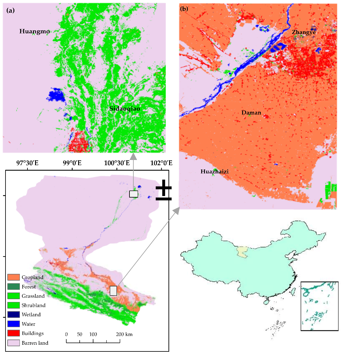
2.1. Study Area

The study areas are located in the midstream (Figure 1a) and downstream (Figure 1b) regions of the HRB. The Heihe River is the second largest inland river in China, which lies in the regions of northwest China, as shown in Figure 1. The latitude of the HRB ranges from 37°42′ to 42°42′N and longitude 97°06′ to 102°00′E, having a unique natural landscape, with land cover types ranging from “ice and snow to frozen soil, forests, rivers, lakes, oases, and the Gobi desert” from south to north [51]. The HRB covers an area of approximately 143,000 km², bordering Ejina Banner in the north, Qilian Mountain in the south, and Dahuang Mountain in the east. Precipitation is scarce in the downstream region, with an annual precipitation of less than 45 mm, and the land in this area is mostly barren land or shrubland. The main crops in the midstream region of the HRB are wheat and maize, and the average annual rainfall and average annual temperature are 136.8 mm and 7.5 °C, respectively [5].

2.2. Data

2.2.1. Satellite Data

Sentinel-2A and Sentinel-2B were successfully launched in June 2015 and March 2017 [52], respectively, having an orbital phase difference of 180° and operating in a sun-synchronous orbit with a height of 786 km and an inclination of 98.5° (https://scihub.copernicus.eu, last accessed: 6 December 2020). A multispectral instrument (MSI) is mounted on the Sentinel-2 satellite, with an imaging width of 290 km, including 13 spectral bands, and a spatial resolution of 10 m, 20 m, or 60 m [53]. Visible and near-infrared bands (Band 2, Band 3, Band 4 and Band 8) are a sensitive canopy structure and suited for vegetation mapping and monitoring [2]. Three spectral bands (Band 5, Band 6 and Band 7) in the leaf-pigment are sensitive to the red-edge part of the electromagnetic spectrum, and bands at 60 m are mainly designed for atmospheric corrections and cloud screening (Band 1 is sensitive to aerosols retrieval; Band 9 is sensitive to water vapor correction, and Band 10 is sensitive to cirrus detection), which have adequate resolution to capture the spatial variability of the atmospheric geophysical parameters [52]. The revisit period of each satellite is 10 days, and the revisit period of both satellites running at the same time is shortened to 5 days. The European Space Agency (ESA) provides Sentinel-2 level-1C products, which can be converted to bottom-of-atmosphere (BOA) reflectance (level-2A) using the Sen2Cor algorithm of atmospheric correction in the SNAP software [53,54]. Then, BOA reflectance values are used as input data to calculate vegetation biophysical parameters, such as the normalized difference vegetation index (NDVI) and fractional canopy coverage (FVC) [55]. The overpass time of Sentinel-2 in the study area is at 12:05 p.m., and the overpass time of Sentinel-3 is uncertain. Therefore, in this study, 18 high-quality Sentinel-3 images during vegetation growing period that were acquired on the same days as the Sentinel-2 images and had an overpass time at approximately 12 p.m. were screened. Images acquired on nine days (25 and 30 June; 15, 25 and 30 July;14 August; 3, 13 and 23 September) in the HRB downstream region and nine days (1 and 16 May; 30 June; 15 and 30 July; 4 and 14 August; 3 and 23 September) in the midstream region were downloaded.

Sentinel-3 is composed of the Sentinel-3A and Sentinel-3B satellites, which were successfully launched in February 2016 and April 2018 [56], respectively. These satellites have a sun-synchronous orbit with an orbital height of 815 km and an orbital inclination of 98.65° and are equipped with an ocean and land color instrument (OLCI), a sea and land surface temperature radiometer (SLSTR), a synthetic aperture radar altimeter (SRAL), and a microwave radiometer (MWR) [57]. The SLSTR can provide reliable global sea surface temperature and land surface temperature data in the forward (55°) observation mode and vertical (0°) observation mode. With its single field of view width (1400 km), the temporal resolution is less than one day, considering the 3A and 3B satellites. In addition, the SLSTR has six VIS-NIR/shortwave infrared channels (S1–S6, spatial resolution: 500 m) and three thermal infrared channels (S7–S9, spatial resolution: 1 km) [58].

2.2.2. Auxiliary Data

The auxiliary data required include land cover classification data and weather-driven data. The classification system of the land cover classification data referred to the International Geosphere-Biosphere Program (IGBP) classification system and the FROM_LC classification system and divided the land cover into 10 categories: cropland, forest, grassland, shrubland, wetland, water bodies, buildings, barren land, glacier, and snow, with an overall accuracy of 92.19% [59,60,61]. The spatial resolution of this dataset is 30 m, and the temporal resolution is one year from 2015 to 2019. In this study, the weather-driven data consisted of wind speed at 10 m, dew point temperature at 2 m, air temperature at 2 m, and surface pressure and total column water vapor data that were obtained from the ERA5 datasets (https://cds.climate.copernicus.eu/, accessed: 12 October 2020). The spatial resolution of the ERA5 datasets was 10 km [62], which was downscaled to 1 km using the bilinear interpolation method to match the spatial resolution of Sentinel-3 LST data, and were used as input parameters to calculate H.

2.2.3. Ground Measurements

The ground measurement data come from the “National Qinghai-Tibet Plateau Scientific Data Center” (http://data.tpdc.ac.cn, accessed: 20 November 2020), including eddy covariance system (EC) data and meteorological data, which are used to validate the results of the retrieved energy balance components [63]. The temporal period of the EC data, which mainly include H, LE, and wind speed et al., was 30 min. Since the observation conditions assume that the land surface is uniform and the atmospheric conditions are neutral, the actual surface conditions are very complicated, and the observed data cannot truly reflect the turbulent characteristics of the region; therefore, the data needed to be corrected, including eliminating the abnormal points, correcting the delay time, rotating the coordinates, and correcting the frequency response. The meteorological data were measured by the automatic weather stations (AWS) with a ten minutes interval, including the net radiation (Rn), soil heat flux(G), meteorological parameters, soil temperature, and humidity. The processing of the meteorological data included removing duplicate data, deleting abnormal data, and unifying the time format [64]. Three ground stations (Zhangye, Daman, and Huazhaizi) in the HRB midstream region and two flux sites (Huangmo and Sidaoqiao) in the HRB downstream region were equipped with EC and AWS. This study extracted ground data according to the Sentinel overpass time. The specific information is shown in

Table 1. Descriptions of the five ground sites.

Station	Longitude (°E)	Latitude (°N)	Altitude (m)	Land Cover Types	Location
Zhangye	100.45	38.98	1460.00	Cropland	Midstream
Daman	100.37	38.86	1556.06	Cropland	Midstream
Huazhaizi	100.32	38.77	1731.00	Barren land	Midstream
Huangmo	100.99	42.11	1054.00	Barren land	Downstream
Sidaoqiao	101.14	42.00	873.00	Shrubland	Downstream

.

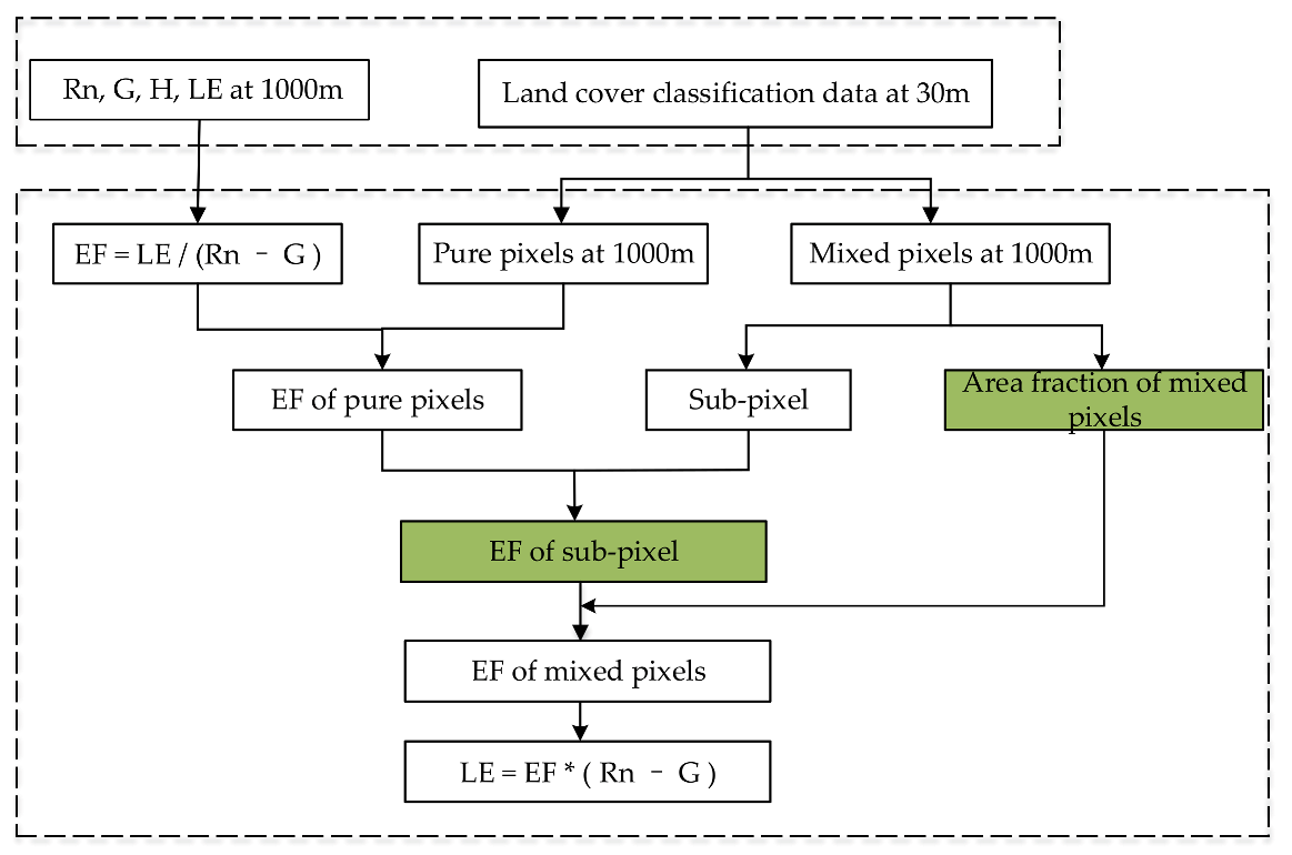
3. Evaporative Fraction and Area Fraction (EFAF) Method

The EFAF method only needs low-resolution energy fluxes and high-resolution land classification data as input data, and its principle is: using high-resolution land classification data to decompose mixed pixels of the coarse-resolution data, and then correcting the EF values of the sub-pixels in the mixed pixels [45], thereby selecting the EF of nearest pure pixels to replace the EF of the sub-pixel to correct the LE values of the mixed pixels. The specific process is as follows:

The EF is usually defined by LE and AE (Rn-G) [65] as follows:

$$\mathrm{EF}=\frac{\mathrm{LE}}{\mathrm{Rn}-\mathrm{G}}$$

(1)

where EF is the evaporative fraction, LE is latent heat flux, $\mathrm{Rn}$ is net radiation, and G is soil heat flux.

Assuming that turbulence occurs only in the vertical direction, the LE of a mixed pixel is weighted by the LE of the sub-pixel, as shown in Equation (2):

$$\mathrm{LE}=\sum {\mathrm{s}}_{\mathrm{i}}{\ast \mathrm{LE}}_{\mathrm{i}}=\sum {\mathrm{s}}_{\mathrm{i}}\ast \frac{{\mathrm{LE}}_{\mathrm{i}}}{{\mathrm{R}}_{\mathrm{n}}-{\mathrm{G}}_{\mathrm{i}}}{\ast \mathrm{R}}_{\mathrm{n}}-{\mathrm{G}}_{\mathrm{i}}=\sum {\mathrm{s}}_{\mathrm{i}}{\ast \mathrm{EF}}_{\mathrm{i}}{\ast \mathrm{R}}_{\mathrm{n}}-{\mathrm{G}}_{\mathrm{i}}$$

(2)

$\mathrm{LE}$ is the accurate LE of mixed pixels, $\mathrm{i}$ denotes the sub-pixel, ${\mathrm{s}}_{\mathrm{i}}$ is the area ratio of the sub-pixel i in the mixed pixel, ${\mathrm{LE}}_{\mathrm{i}}$ represents the LE of sub-pixel i in a mixed pixel, and ${\mathrm{R}}_{\mathrm{n}}-{\mathrm{G}}_{\mathrm{i}}$ and ${\mathrm{EF}}_{\mathrm{i}}$ are the AE and EF of sub-pixel i.

It is assumed that the AE of each sub-pixel is equal and equal to the AE of the entire mixed pixel; therefore, Equation (2) can be transformed into:

$$\widetilde{\mathrm{LE}}=[\sum {\mathrm{s}}_{\mathrm{i}}{\ast \mathrm{EF}}_{\mathrm{i}}]\ast \left({\mathrm{R}}_{\mathrm{n}}-\mathrm{G}\right)$$

(3)

$\widetilde{\mathrm{LE}}$ is the LE of a mixed pixel under the assumptions, which has a minor error with $\mathrm{LE}$.

Combined with Equation (1), Equation (3) can be transformed into:

$$\widetilde{\mathrm{EF}}=\frac{\widetilde{\mathrm{LE}}}{\left({\mathrm{R}}_{\mathrm{n}}-\mathrm{G}\right)}=\sum {\mathrm{s}}_{\mathrm{i}}{\ast \mathrm{EF}}_{\mathrm{i}}$$

(4)

where $\widetilde{\mathrm{EF}}$ is the EF of a mixed pixel assuming that the AE of sub-pixels are equal in that mixed pixel. Assuming that the EF of sub-pixel i of a certain land type in a mixed pixel is equal to the EF of the nearest pure pixels of this land cover type, the EF of sub-pixel i can be replaced by the EF of the pure pixels to obtain the EF of the mixed pixel.

Incorporating Equation (4) into Equation (3), Equation (5) is obtained:

$$\widetilde{\mathrm{LE}}=\widetilde{\mathrm{EF}}\ast \left({\mathrm{R}}_{\mathrm{n}}-\mathrm{G}\right)$$

(5)

Equation (5) shows that the EFAF method uses the EF of the sub-pixels in the mixed pixel as a bridge and achieves the goal of correcting LE by correcting the EF.

The following is a simple example to illustrate the EFAF method. In Figure 2, A, B, and C denote different land cover types, where pixel 1, pixel 2, and pixel 4 are pure pixels, whereas pixel 3 is a mixed pixel. The EF of A in pixel 1, EF of B in pixel 2, and EF of C in pixel 4 are used to replace the EF of A, EF of B, and EF of C, respectively, in pixel 3; thus, the EF of pixel 3 is obtained, which is then multiplied by the AE of pixel 3 to acquire the corrected LE.

The flowchart for correcting the LE based on the EFAF method is shown in Figure 3. First, calculate a 1 km spatial resolution EF through energy fluxes. Then, resample the 30 m spatial resolution land classification data to 1 km according to the area ratio, and count pure pixels and mixed pixels in the 1 km land classification data. Meanwhile, obtain the sub-pixels land cover types and their area ratios according to the mixed pixels. The next step is to obtain the EF of each pure pixel through the EF data and the pure pixel data, and to then replace the EF of the sub-pixel in the mixed pixel with the EF of the nearest pure pixels of same land cover type, so that the corrected EF of the mixed pixel is obtained after area weighting. When the spatial resolution of the data is large, there is a possibility that no pure pixels can be found, so new measures need to be adopted. This topic is discussed in Section 6.2. Finally, the corrected EF is multiplied by the AE to obtain the corrected LE.

4. Parameter Retrieving and ET Estimation

4.1. Parameter Retrieving

The parameters required by the ET model are calculated using Sentinel-2 and Sentinel-3 data.

NDVI is an essential component of any study aiming to investigate ecosystem services, especially those where vegetation, water, and biodiversity are involved [66]. For example, NDVI is a sensitive indicator of canopy structure, which can monitor vegetation growth [67], and its utility in indicating the soil moisture has been well demonstrated over the past two decades [68]. The NDVI products derived from moderate-resolution imaging spectroradiometer (MODIS) [69], advanced very high-resolution radiometer (AVHRR) [70] and Himawari-8 [71] have provided moderate- to low-resolution NDVI time series globally, and have been widely applied in studying dynamic monitoring, vegetation phenology, and global change [72]. However, widespread contamination (due to aerosols, clouds, etc.) and the long revisit period of these high-resolution satellites induce large gaps in the NDVI time series data and limit their application in related studies [73].

From the Sentinel-2 level-2A data, NDVI was retrieved through the B4 band (red) and B8 band (near-infrared), as shown in Equation (6).

$$\mathrm{NDVI}=\frac{{\mathsf{\rho }}_{nir}-{\mathsf{\rho }}_{red}}{{\mathsf{\rho }}_{nir}+{\mathsf{\rho }}_{red}}$$

(6)

where ${\mathsf{\rho }}_{nir}$ is the reflectance in the near-infrared band and ${\mathsf{\rho }}_{red}$ is the reflectance in the red band.

The calculation of the FVC and leaf area index (LAI) was carried out through the Biophysical Processor in SNAP software. First, the Sentinel-2 level-2A product needed to be resampled by SNAP software to unify the spatial resolution of each band to 10 m, and then eight band data (B3–B7, B8a, B11, and B12) were input into the Biophysical Processor module in SNAP software. Finally, FVC, LAI, and their quality indicators were automatically obtained [54]. The Biophysical Processor module combined the PROSPECT+SAIL coupled radiation transmission model with an artificial neural network [2]. Its procedure to derive LAI and FVC was: using the PROSPECT model to simulate the upward and downward radiant flux of leaves to obtain the reflectance and transmittance of vegetation leaves; using the SAIL model to combine the reflectance and transmittance of vegetation leaves with environmental parameters, such as soil reflectivity and solar altitude angle, as input data, thus obtaining the vegetation canopy reflectance data. The vegetation canopy reflectance and eleven parameters, such as the zenith angle, were used as the input layer, and LAI and FVC were obtained through the back propagation artificial neural network [55].

The surface albedo was calculated from Sentinel-2 data using an algorithm (Equation (7)) proposed by Bonafoni (2020) [74]. The algorithm was simple, directly converting the surface reflectance to surface albedo, and required images acquired in clear and cloudless conditions. The root mean square error (RMSE) of this algorithm was good, with an average error of approximately 0.02.

$$\begin{gathered} \mathsf{\alpha }=0.2266\ast {\mathsf{\rho }}_{B2}+0.1236\ast {\mathsf{\rho }}_{B3}+0.1573\ast {\mathsf{\rho }}_{B4} \\ +0.3417\ast {\mathsf{\rho }}_{B8}+0.1170\ast {\mathsf{\rho }}_{B11}+0.0338\ast {\mathsf{\rho }}_{B12} \end{gathered}$$

(7)

where $\mathsf{\alpha }$ is the albedo, and ${\mathsf{\rho }}_{B2}$, ${\mathsf{\rho }}_{B3}$, ${\mathsf{\rho }}_{B4}$, ${\mathsf{\rho }}_{B8}$, ${\mathsf{\rho }}_{B11}$, and ${\mathsf{\rho }}_{B12}$ denote the surface reflectance of Band 2, Band 3, Band 4, Band 8, Band 11 and Band 12.

However, it should be noted that Sentinel-2 BOA reflectance spectra were overestimated using the Sen2Cor algorithm [75], which affects the Rn and the albedo [76].

The algorithm for retrieving LST using Sentinel-3 data was provided by Li [77]. First, the vegetation cover method was used to estimate the surface emissivity, and then a modified generalized split-window (SW) algorithm was used to calculate LST. The algorithm was used to produce synergized quantitative (MuSyQ) LST products using MODIS TIR data. Sentinel-3 LST derived from this algorithm was validated with ground observed data from five sites in the study area, and the evaluation results shown that Sentinel-3 LST was overestimated, with the coefficient of determination (R²) being 0.94, MBE being 2.7 K, and RMSE being 3.47 K.

Zhou (2007) [78] proposed a new empirical model with nonlinear parameterization for calculating downward longwave radiation (DLR) based on the original Zhou–Cess algorithm, which needs 2 m air temperature and column water vapor (CWV) from ERA5 datasets as input data. As a result of the convenience of the input data, using this model to calculate DLR is easy, and it would expand the applicability of remote sensing in the field of energy balance. The retrieved DLR was validated using ground measurement data in the study area, and its evaluation results show that the accuracy of the DLR was good. The MBE is 9.1 W/m² and RMSE is 36.5 W/m².

Zhang [79] provided an effective algorithm for calculating downward shortwave radiation (DSR) from Sentinel-2 data by employing look-up tables (LUT). First, the radiation transmission model was used to construct a DSR array corresponding to different atmospheric and surface conditions, and the dimensions of the DSR array were reduced and interpolated to obtain the look-up table. Then, Sentinel-2 B2, B3 and B4 bands were used to calculate the aerosol optical depth (AOD) and cloud optical depth (COD). Finally, the DSR was retrieved using the LUT according to the AOD and COD. The estimated DSR was compared against ground measurements collected from five stations in the HRB midstream region and downstream region, and the validation results achieved R² values of 0.8, MBE of 18.1 W/m², and RMSE of 37.05 W/m².

4.2. ET Estimation

Before using the EFAF method to correct the LE, the Rn, G, H, and LE are estimated using an input parameter upscaling (IPUS) algorithm. The spatial resolutions of TIR data and VIS-NIR data are quite different, and there are no TIR data that can match the high spatial resolution of VNIR data. Therefore, Sentinel-2 and Sentinel-3 data face the problem of spatial scale mismatching. The IPUS algorithm is an energy balance single-source model that upscales high-resolution parameters to the same spatial resolution as LST data to calculate energy components [31], thus solving the problem of mismatches in the resolutions of satellite data.

Rn controls the AE used by vegetation and land for ET and is calculated based on incoming radiation and outgoing radiation, as shown in Equation (8).

$${\mathrm{R}}_{\mathrm{n}}={\mathrm{S}}_{\mathrm{d}}\ast \left(1-\mathsf{\alpha }\right)+{\mathsf{\epsilon }}_{\mathrm{s}}{\ast \mathrm{L}}_{\mathrm{d}}-{\mathsf{\epsilon }}_{\mathrm{s}}{\ast \mathsf{\sigma }\ast \mathrm{T}}_{\mathrm{rad}}{}^4$$

(8)

where ${\mathrm{S}}_{\mathrm{d}}$ denotes DSR; $\mathsf{\alpha }$, ${\mathsf{\epsilon }}_{\mathrm{s}},$ and $\mathsf{\sigma }$ are the land albedo, land emissivity, and Stephen–Boltzmann constant, respectively; ${\mathrm{L}}_{\mathrm{d}}$ is DLR; and ${\mathrm{T}}_{\mathrm{rad}}$ is LST.

For water bodies, G is usually equal to a ratio of Rn (0.226). For buildings such as towns and roads, G is derived using an algorithm (Equation (9)) from the objective hysteresis model (OHM) [80,81]:

$${\mathrm{G}}_{soil}={\mathrm{a}}_1{\ast \mathrm{R}}_{\mathrm{n}}+{\mathrm{a}}_2\ast \frac{\partial {\mathrm{R}}_{\mathrm{n}}}{\partial t}+{\mathrm{a}}_3$$

(9)

where ${\mathrm{a}}_1$ is 0.85, ${\mathrm{a}}_2$ is 0.32 and its unit is in hours, and ${\mathrm{a}}_3$ is −28.5 and its unit is in W/m².

In other cases, G is obtained based on its relationship with FVC as follows:

$$\mathrm{G}={\mathrm{R}}_{\mathrm{n}}\ast \left[{\mathsf{\Gamma }}_{\mathrm{c}}+\left(1-{\mathrm{f}}_{\mathrm{c}}\right)\ast \left({\mathsf{\Gamma }}_{\mathrm{s}}-{\mathsf{\Gamma }}_{\mathrm{c}}\right)\right]$$

(10)

where the value of ${\mathsf{\Gamma }}_{\mathrm{s}}$ is 0.05 for full vegetation, the value of ${\mathsf{\Gamma }}_{\mathrm{c}}$ is 0.315 for bare soil, and ${\mathrm{f}}_{\mathrm{c}}$ is FVC [12].

Equation (11), which requires many parameters and is based on the gradient diffusion theory, is used to calculate H [82]:

$$\mathrm{H}={\mathsf{\rho }\mathrm{c}}_{\mathrm{p}}\frac{{\mathrm{T}}_{\mathrm{aero}}-{\mathrm{T}}_{\mathrm{a}}}{{\mathsf{\gamma }}_{\mathrm{a}}}$$

(11)

where H is sensible heat flux, $\mathsf{\rho }$ represents the density of air, ${\mathrm{c}}_{\mathrm{p}}$ denotes specific heat of air constant pressure, ${\mathrm{T}}_{\mathrm{aero}}$ and ${\mathrm{T}}_{\mathrm{a}}$ are the aerodynamic surface temperature and the air temperature at the reference height, respectively, and ${\mathsf{\gamma }}_{\mathrm{a}}$ is the aerodynamic resistance, which was calculated through the Monin–Obukhov similarity theory (MOST) utilizing a stability correction function [83,84]. The zero-plane displacement height and roughness length were parameterized by the schemes proposed by Choudhury and Monteith [85]. The reference height is generally 2 m above the land surface [44], so ${\mathrm{T}}_{\mathrm{a}}$ is air temperature at 2 m above the land surface, which is provided by ERA5 datasets.

Due to the special surface of the buildings, LE was assumed to be zero over impervious surfaces and the H of urban areas was calculated by subtracting G and LE from Rn (H = Rn − G − LE) [45,86].

In other cases, the $\mathrm{LE}$ is estimated as the residual of the energy balance (Equation (12)). More details can be found in the study by Peng et al. (2016) [31].

$$\mathrm{LE}={\mathrm{R}}_{\mathrm{n}}-\mathrm{G}-\mathrm{H}$$

(12)

The ET values estimated by the IPUS algorithm were used as input data for the EFAF method and compared with the corrected ET values.

5. Results

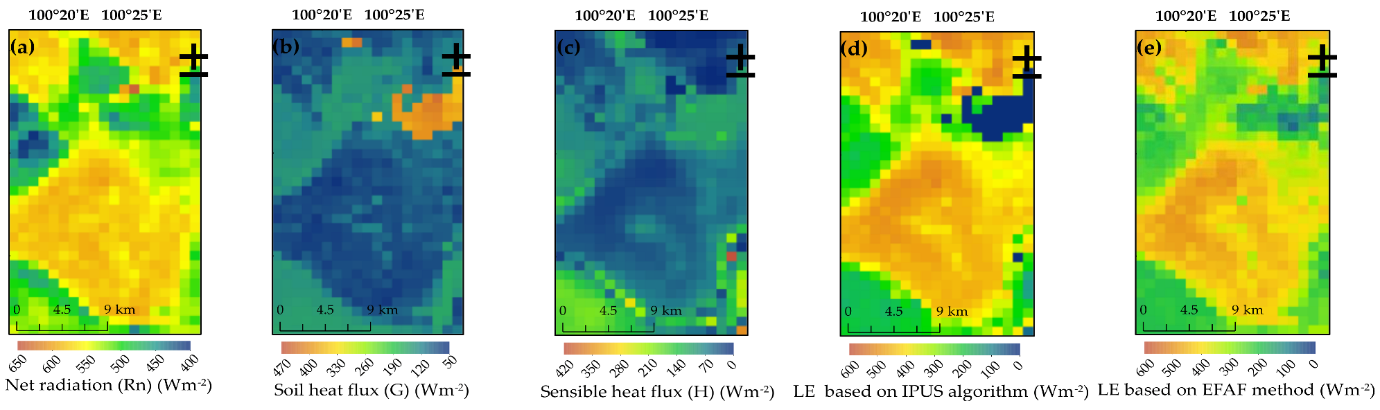
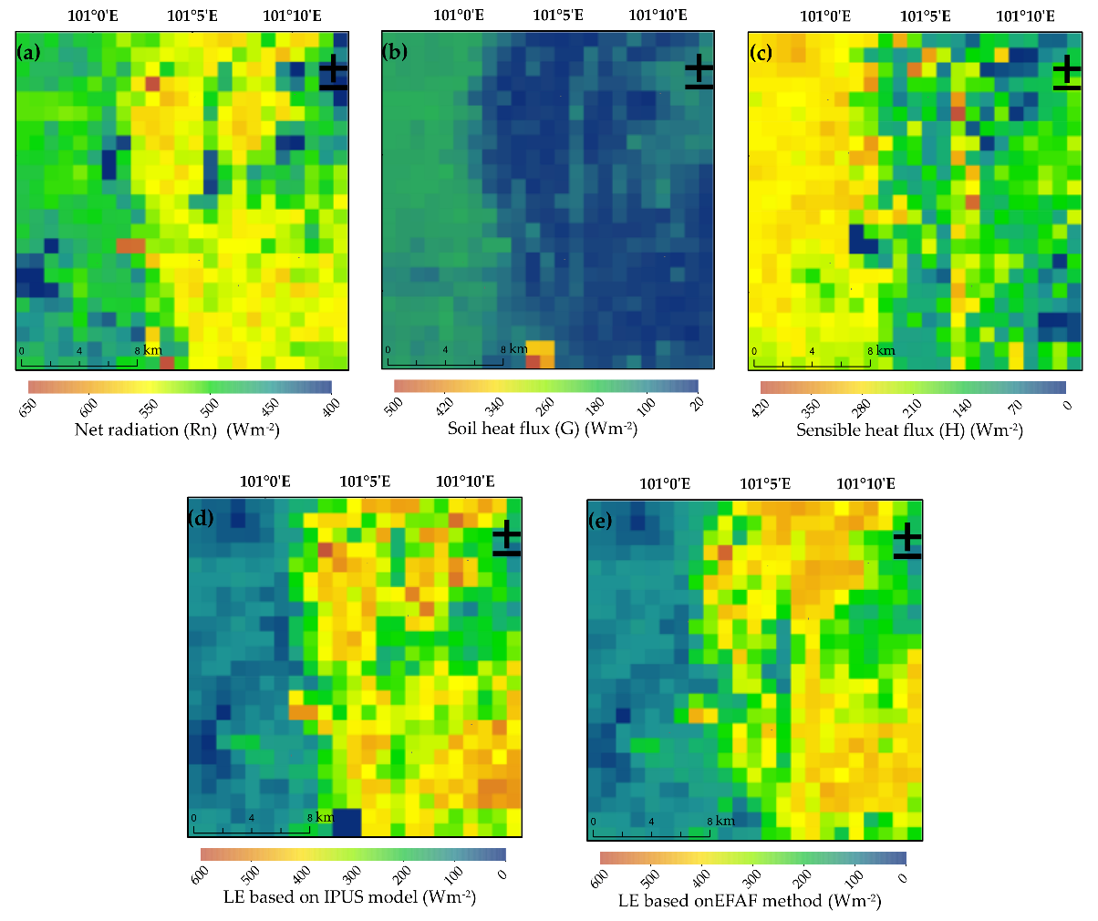
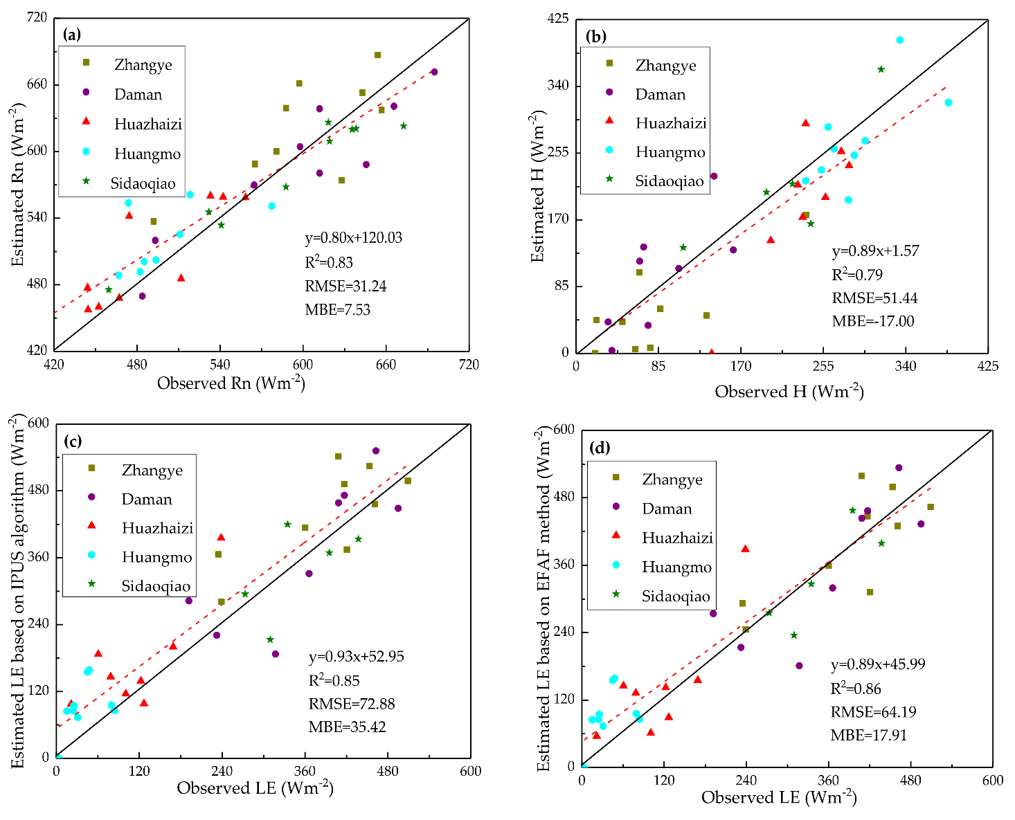
5.1. Results of the Energy Flux

Figure 4 and Figure 5 show the results of the energy flux with a 1 km resolution on 14 August 2019 in the HRB midstream and HRB downstream regions, respectively. The energy flux has obvious spatial distribution characteristics and great similarities with the land cover classification. The reasons for these findings are that the phenological conditions of the same feature type are similar, as are the values of the land surface parameters and the estimated energy fluxes. In the study area, the Rn and LE values of the cropland are slightly higher than those of the shrubland, whereas the Rn and LE values of the barren land are lower. The H of barren land is higher than that of cropland and shrubland. The spatial distribution of the four energy components is reasonable. Comparing Figure 4d,e and Figure 5d,e, it can be seen that the LE has obvious changes in local areas after being corrected. Figure 6 is a scatter plot of the LE based on the IPUS algorithm and EFAE method on 14 August 2019 for different land types in the study area, and the land cover types are mainly cropland, shrubland, and barren land. Among them, the cropland is mainly distributed in the midstream region, and its LE has generally decreased. In contrast, shrubland is mainly distributed in the downstream region, and its LE varies greatly, ranging from approximately −120 W/m² to 120 W/m². Barren land is in the midstream and downstream regions, and its LE has both increased and decreased. It should be noted that the ERA5 datasets are inappropriate over built-up surfaces [87,88] and the ET is based on evaporation from soil and transpiration from vegetation [89]; thus, the LE of buildings is not considered here.

Figure 7 is a box plot of the EFs of different feature types throughout the study area on 14 August 2019. The blue boxes represent the EFs of the mixed pixels before correction, the yellow boxes are the EFs of the searched nearest pure pixels corresponding to the sub-pixels of the mixed pixels before correction, and the green boxes represent the distribution of the EFs of the mixed pixels after correction. In general, the EFs of the pure pixels in the cropland were slightly lower than those of the sub-pixels in mixed pixels, which will reduce the EFs of the cropland pixels after being corrected. Moreover, cropland has the largest EF exception of the water bodies, so the sub-pixels of other ground features in cropland mixed pixels will also reduce the EF of the cropland pixels. Therefore, the EF and LE values will eventually decrease.

Table 2. LE and EF of three pixels with different underlying surfaces.

Pixel	Underlying Surface	LE-Observed (W/m2)	LE-IPUS (W/m2)	EF-IPUS	LE-EFAF (W/m2)	EF-EFAF
Pixel 1	Cropland	416.98	492.06	0.99	447.33	0.90
Pixel 2	Shrubland	437.38	393.5	0.72	398.97	0.73
Pixel 3	Barren land	169.15	199.97	0.58	155.15	0.45

shows the LEs and EFs of three pixels with different underlying surfaces, and

Table 3. The area ratios and changes in the EF of the sub-pixels in the mixed pixels.

Pixel	Land Cover Types	Area Ratio	EF
Pixel 1	Cropland	0.7591	0.97
	Forest	0.0189	0.99
	Grassland	0.0558	0.74
	Wetland	0.066	0.99
	Water bodies	0.0105	1.00
	Buildings	0.0108	0.00
	Barren land	0.0789	0.34
Pixel 2	Shrubland	0.6706	0.87
	Barren land	0.3294	0.46
Pixel 3	Barren land	0.9982	0.45
	Cropland	0.0018	0.81

shows the area ratios and changes in the EFs of the sub-pixels in the mixed pixels. The pixel (Figure 8, pixel 1) in which the Zhangye site is located is used as an example to illustrate the changes in the LE in the mixed cropland pixels. When the IPUS algorithm estimated the LE, the underlying surface of the entire pixel was regarded as cropland, and the estimation of EF was 0.99 and the LE was 492.06 W/m², which were higher than the observed data. In fact, pixel 1 contained seven types of ground features, among which, the EF and LE of forest and wetland did not change because they did not have corresponding pixels in the 1 km land classification data. The EFs of pure pixels of cropland, grassland, and barren land were all less than 0.99. The values of the EF and LE ultimately decreased after area weighting, and the overestimation of the LE in pixel 1 was partially corrected.

Shrubland is distributed in the downstream region, and its mixed pixels are mainly mixed with barren land, which will reduce the EFs of the shrubland pixels after being corrected. When the EF of the nearest found pure shrubland pixels was smaller than the EF of the shrubland sub-pixel in the mixed pixel, the EF of the mixed pixel decreased, and the LE also decreased. When the area ratio of shrubland in the mixed pixels was much larger than that of barren land, and if the EF of the nearest found pure shrubland pixels was greater than the EF of the shrubland sub-pixel, the EF and LE of the mixed pixel became larger. The pixel (Figure 8, pixel 2) in which the Sidaoqiao site is located is used as an example to show the change in LE in a shrubland mixed pixel. The LE of pixel 2 estimated by the IPUS algorithm was 393.5 W/m², which was lower than the ground station value of 437.38 W/m². Pixel 2 contains barren land and shrubland, the area ratios of which are 0.3294 and 0.6706, respectively, and the EFs of the searched nearest pure pixels are 0.46 and 0.87, respectively. The corrected LE was 398.97 W/m², which was closer to the observed data; thus, the underestimation of LE in pixel 2 was partially corrected.

In barren land, the difference between the average EF of the pure pixels and the average EF of the mixed pixel was −0.2, which will reduce the EFs of the barren land pixels after being corrected. The EFs of the cropland and shrubland were larger than those of the barren land, and most of the barren land was mixed with these two types of land cover, thus increasing the EF in barren land mixed pixels. When the area ratio of the barren land in mixed pixels was much larger than that of the other land cover types, and if the EF of the sub-pixel of barren land is greater than the EF of the nearest pure pixels of barren land, the EF and LE of the mixed pixel decreased, otherwise, the EF and LE increased. When the area ratio of the mixed pixels dominated by barren land was slightly more than that of the cropland and shrubland, and if the EF of the barren land pure pixel was smaller than that of sub-pixel, and the EF of pure pixel of cropland and shrubland is greater than that of the sub-pixel, and the EF change in the barren land was greater than that of the cropland and shrubland, the EF and LE of the mixed pixels became smaller. Otherwise, the EF and LE became larger. The change in the LE of the pixel (Figure 8, pixel 3) where the Huazhaizi site is located on 14 August 2019 explains the correction process applied for the barren land. The area ratio of the barren land in pixel 3 was much higher than that of the cropland, so the impact of cropland on the change in the EF was negligible. The EF of the searched nearest pure pixels was smaller than the estimated EF of the pixel, so the EF and LE of pixel 3 decreased.

The box plot and examples of these three pixels prove that the changes in LE are reasonable, showing that the EFAF method is suitable for correcting the error of LE estimated with 1 km resolution Sentinel data caused by land surface heterogeneity.

5.2. Validation

The ground measurement data were corrected by the Bowen ratio method for energy closure and then compared against the estimated Rn, H, and LE values. The results are shown in Figure 9. The R², RMSE, and MBE of Rn were 0.83, 31.24 W/m², and 7.53 W/m², respectively, and the R², RMSE, and MBE of H were 0.79, 51.44 W/m², and −17.00 W/m², respectively. Compared with those of the Rn and H, the RMSE and MBE of the LE were larger, with the RMSE ranging between 60 and 80 W/m² and MBE ranging between −15 and 60 W/m². Due to the fact that the LE was calculated through the remainder of the energy balance, the errors in the Rn and H accumulated to the LE. Figure 9 shows that these errors are within a reasonable range. The LE value of the pixel where the Huangmo site is located did not change because this pixel is a pure pixel. The EFAF method corrects only mixed pixels and does not correct pure pixels. After using the EFAF method to correct the LE estimated by the IPUS algorithm, the ground data and the estimated values were closer to the 1:1 line, indicating that the accuracy of the LE improved.

Table 4. The station validation results of the LE.

Station	Method	R2	MBE (W/m2)	RMSE (W/m2)
Zhangye	IPUS	0.60	49.37	76.47
	EFAF	0.61	7.17	60.93
Daman	IPUS EFAF	0.66 0.66	7.69 −4.58	72.53 70.17
Huazhaizi	IPUS EFAF	0.61 0.65	57.43 31.35	81.35 68.18
Huangmo	IPUS/EFAF	0.19	53.02	66.51
Sidaoqiao	IPUS	0.36	−12.20	62.73
	EFAF	0.70	−11.44	46.66

Note: R² is the coefficient of determination; RMSE is the root mean square error; MBE is the mean bias error.

shows the R², MBE, and RMSE of the observation compared with the LE estimated by the IPUS algorithm and EFAF method. The LEs of the Zhangye and Daman sites were generally high. The EFAF method added the contributions of other land cover types into the mixed pixels, so the overestimation of LE was corrected. The error in the LST at the Huazhaizi site was relatively large, which led to the estimated Rn being higher and the estimated H being lower than ground data. The errors in the Rn and H accumulated to the LE, ultimately causing the error in the LE to be relatively large. The performance of the EFAF method was superior to that of the IPUS algorithm, with the R² increasing and RMSE decreasing, the MBE decreasing by 17 W/m² on average, and the LE value becoming more concentrated. Section 5.1 shows that the EFAF method performs well when correcting the LE, and the corrected LE values are closer than the LE values before correction to the observed values. Therefore, the EAFA method can address the problem of land surface heterogeneity and can correct the error of LE with coarse resolution remote sensing and obtain more accurate LE values than the IPUS algorithm.

It is worth pointing out that the scale matching between the coarse pixel estimate and the source area of the EC measurements needs to be addressed. In this study, the pixel where the Huangmo site is located is a pure pixel and the pixels where the other four sites (Zhangye, Daman, Huazhaizi, and Sidaoqiao) are located are mixed pixels. Research shows that the main EC source areas were within a radius of 250 m [64]. It can be known from the positions of the four sites in the pixels where they are located: the source areas of the Huazhaizi and Sidaoqiao sites are in the pixels where the sites are located. The locations of the Zhangye and Daman sites are at the edge of the mixed pixels, and their source areas include the adjacent pixels areas of the pixels where the sites are located. Therefore, when verifying with the ground measurements, the estimations of the pixel where the site is located and the estimations of the adjacent pixels need to be averaged, and then compared with the EC measurements.

In addition, given that reliable ground measurements are restricted by many factors, such as complex conditions (for example, topography and unfavorable weather) [64], 30 min EC estimates have large uncertainty and may influence the validation results of LE. To further justify the EFAF method, daily LE measurements were aggregated using a range of time series LE estimates based on the time at which Rn shifted from positive to negative values. The LE calculated by the IPUS algorithm and the LE corrected by the EFAF method [45] were extrapolated to the daily scale based on the EF method for validation. The results are shown in

Table 5. The station validation results for the daily LE.

Station	Method	R2	MBE (MJ/m2)	RMSE (MJ/m2)
Zhangye	IPUS	0.66	0.53	2.95
	EFAF	0.69	−1.01	2.83
Daman	IPUS EFAF	0.85 0.85	2.44 2.00	2.82 2.43
Huazhaizi	IPUS EFAF	0.79 0.88	3.05 2.32	3.84 3.41
Huangmo	IPUS/EFAF	0.10	2.83	3.30
Sidaoqiao	IPUS	0.28	1.15	2.43
	EFAF	0.36	1.13	2.31

. It can be seen that the MBE varies from −1 to 3 MJ/m², the RMSE ranges from 2.5 to 3.5 MJ/m², and the error of the validation results of the EFAF method is smaller. In general, the daily LE based on the EFAF method is more consistent with the EC measurements than the daily LE estimated on the IPUS algorithm.

6. Discussion

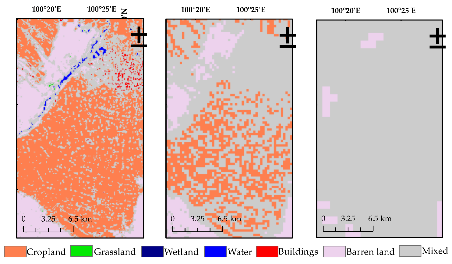
6.1. Sensitivity Analysis of the Land Cover Map with the EFAF Method

High-resolution land classification data are the basis for identifying pure pixels [45] and mixed pixels and decomposing mixed pixels in coarse-resolution data, which play a particularly vital role in the EFAF method. Therefore, it is necessary to analyze the influence of land classification data on the EFAF method.

Because the EFs of the sub-pixels in the mixed pixel are replaced by the EFs of the searched nearest pure pixels, it is necessary to calculate the average EFs of the pure pixel before correction for different land types when analyzing the sensitivity of the land cover map. The average EF values of the pure pixels of cropland, barren land, and shrubland on 14 August 2019, calculated before correction for the entire study area, were 0.82, 0.26, and 0.81, respectively, and the EFs of the water bodies and buildings were defined as 1 and 0, respectively. In addition, the average AE of all of the pixels in the entire study area was determined to be 463.98 W/m².

Misclassification caused the EF and area ratios of sub-pixels within mixed pixels to be incorrect, which further led to deviations in the LE.

Table 6. Differences in EF and LE caused by incorrect classification. “+” means overestimation and “−” means underestimation.

Incorrect Classification	EF or LE (Wm−2)	Correct Classification
		Cropland	Barren Land	Shrubland	Water Bodies	Buildings
Cropland	EF	0	+0.56	+0.01	−0.18	+0.82
	LE	0	+259.83	+4.64	−83.52	+380.46
Barren land	EF	−0.56	0	−0.55	−0.74	+0.26
	LE	−259.83	0	−255.19	−343.35	+120.64
Shrubland	EF	−0.01	+0.55	0	−0.19	+0.81
	LE	−4.64	+255.19	0	−88.16	+375.82
Water bodies	EF	+0.18	+0.74	+0.19	0	+1
	LE	+83.52	+343.35	+88.16	0	+463.98
Buildings	EF	−0.82	−0.26	−0.81	−1	0
	LE	−380.46	−120.64	−375.82	−463.98	0

shows the difference between the EF and LE when the land cover types are misclassified. In this table, “+” means overestimation and “−” means underestimation. The error caused by the misclassification of cropland and shrubland was the smallest, because these land cover types have similar phenological conditions. Incorrectly classifying barren land as cropland and shrubland caused the LE to be overestimated by 259.83 W/m² and 255.19 W/m², respectively. Furthermore, the EF and LE were generally underestimated when water bodies were incorrectly classified as other land cover types because their EFs were the largest. Conversely, the EF and LE were generally overestimated when buildings were misclassified as other land cover types, as the EF of buildings was the smallest. The error caused by the incorrect classification of water bodies and buildings was relatively large, but their spectral characteristics were obviously different from those of the other land cover types, so the probability of misclassification was low.

6.2. Adjustments for Selecting Pure Pixels at Coarse Resolution

When using the EFAF method to correct LE values, it is necessary to select the EFs of the pure pixels to replace the EFs of the sub-pixels in the mixed pixels. The selection of the pure pixels plays an important role in correcting the LE values.

The choice of pure pixels is closely related to the spatial scale of the images being used. The higher the image spatial resolution, the greater the number of pure pixels, the shorter the search distance for pure pixels, and the greater the probability that pure pixels can be found. Li [34] used the EFAF method to correct LE values at a spatial resolution of 300 m, whereas this research needs to correct LE values at a resolution of 1000 m. The high-resolution land classification data in the HRB midstream region were resampled to 100 m (Figure 10, left), 300 m (Figure 10, middle), and 1000 m (Figure 10, right) in order to compare and analyze the availability of pure pixels at different spatial scales. The proportions of pure pixels in the land classification data with a spatial resolution of 100 m and 300 m were both greater than 40% (

Table 7. Proportions of pure pixels and mixed pixels at different spatial scales.

Spatial Scale (m)	Proportion of Pure Pixels (%)	Proportion of Mixed Pixels (%)
100 m	71.73	28.27
300 m	40.5	59.5
1000 m	5.4	94.6

), and a large number of pure pixels were distributed around the mixed pixels; therefore, the sub-pixel can easily find the corresponding same land cover type pure pixels. In contrast, when the spatial resolution was 1000 m, pure pixels were available for only barren land. The cropland, which accounts for a large proportion of the study area, had no pure pixels, so the EF of the cropland sub-pixels in the mixed pixels could not be replaced by the EF of pure pixels, and LE was not corrected or changed. Therefore, the EFAF method of selecting pure pixels at a coarse resolution needs to be adjusted.

When pure pixels are not found within a limited search range, the standard for identifying pure pixels needs to be lowered according to the spatial resolution. Cropland provides an example of the process of adjusting the strategy for selecting pure pixels. There were no pure pixels of cropland in the entire study area, and a total of 573 pixels included sub-pixels of cultivated land. The adjusted area ratio of pure pixels should be as close to 1 as possible, so, starting from 1 and decreasing by 0.01, the number of pixels with different area ratios was counted. The number of pixels with cropland area ratios greater than 0.99, 0.98, and 0.97 was 26, 74, and 116, respectively. The EFAF method does not correct the LEs of pure pixels. Therefore, if pixels with an area ratio greater than 0.97 are regarded as pure pixels, the LEs of 20% of the pixels will not change. This ratio is obviously unsuitable. In addition, the number of pixels with an area ratio greater than 0.99 was less than 5%. If the number of pure pixels is too small, the distances between sub-pixels and the searched nearest pure pixels may be too large. Although pure pixels are found, their phenological conditions may be very different from those in the mixed pixels. Therefore, pixels with a ratio of cropland greater than 0.98 were selected as pure pixels, and the result is shown in Figure 11. After adjusting the strategy of searching for pure pixels, pixel 1 (Figure 11, top) could search for pure pixels at a search distance of six cells, and pixel 2 (Figure 11, bottom) could find pure pixels at a search distance of two cells. The EFs of the cropland sub-pixels in the study area were replaced by the EFs of the pure pixels within 10 cells, so as to achieve the purpose of correcting LE. The criteria for finding pure pixels for other land cover types are similar to those for cropland. For a land cover type that has no pixels in the entire study area, its sub-pixel EF would not change.

6.3. Uncertainty of Energy Balance Closure Method with EFAF Method

The sum of the H and LE observed by the five EC sites is less than the available energy (AE, the difference between the Rn and G), and energy imbalances are common in ground measurement data [90]; thus, this study used the Bowen ratio closure method for energy closure on the ground measurement data. Traditionally, both the Bowen ratio closure method and residual LE closure method can be used for energy closure. The Bowen ratio closure method assumes that the ratio of H to LE (Bowen ratio) is correctly measured by the EC system, and then uses the Bowen ratio to divide the AE so that the values of H and LE can be adjusted [91]. The residual LE closure method assumes that H is accurately measured, and LE is obtained by subtracting H from the AE and serves as boundary conditions to account for the extreme cases [92,93]. Both methods have advantages and characteristics, and there is no evidence that either method performs better than the other [90]. To better contextualize the uncertainties of closure methods on the present study, some discussion about the differences between the Bowen ratio closure method and residual LE closure method is warranted.

The ground measurement data were corrected by the Bowen ratio closure method and residual LE closure method and then compared against the estimations of H and LE based on remote sensing data. The validation results of the two methods are presented in

Table 8. The validation results based on the Bowen ratio closure method and residual LE closure method.

Energy Flux	Closure-Method	R2	MBE (W/m2)	RMSE (W/m2)
H	Bowen ratio closure	0.79	−17.00	51.44
	Residual LE closure	0.51	15.49	74.56
IPUS-LE	Bowen ratio closure	0.85	35.42	72.88
	Residual LE closure	0.76	15.87	83.67
EFAF-LE	Bowen ratio closure	0.86	17.91	64.19
	Residual LE closure	0.80	−1.63	74.01

. The sum of the ground measurement data H and LE is less than the difference between the Rn and G; thus, the Bowen-ratio-corrected LE (BRLE) and H (BRH) increase, and the residual-LE-corrected LE (RELE) increase, whereas H (REH) does not change. Compared with the H estimated from remote sensing data, the MBE of BRH is −17.00 W/m², indicating that the estimated His less than the mean of BRH. Since the BRH is greater than REH, the MBE between estimations of H and REH increases, being 15.49 W/m². The error between the BRH and estimations of H is smaller than the LEH and estimations of H. The BRLE is less than RELE; thus, the MBE of BRLE is greater than the MBE of RELE. Compared with the LE based on the IPUS algorithm and EFAF method, the RMSE of BRLE is approximately 20 W/m² higher than that of RELE, whereas the MBE of BRLE is approximately 10 W/m² lower than that of RELE. Moreover, the error of the LE corrected by the EFAF method is smaller than the error of the LE estimated on the IPUS algorithm corrected by either the Bowen ratio closure method or residual LE closure method. Overall, regardless of whether the ground measurement data are corrected by the Bowen ratio closure method or residual LE closure method, the performance of the EFAF method is superior to that of the IPUS algorithm.

7. Conclusions

As a satellite that has been launched in the past two years, Sentinel data have great advantages in temporal and spatial resolution. Images from these satellites can be continuously acquired for a long period of time in the future and have great application potential for the long-term detection of the surface energy balance. In this research, Sentinel-2 and Sentinel-3 data provided the parameters required by the IPUS algorithm to estimate LE. The IPUS algorithm assumes that there is only one land cover type in a single pixel when calculating the LE, whereas the EFAF method considers that there may be multiple land cover types in pixels and adds the contributions of sub-pixels of different land cover types to the mixed pixels, thereby correcting estimations of the LE of mixed pixels. This study proved that the EFAF method is suitable for correcting the deviation in LE estimated based on Sentinel data caused by land surface heterogeneity. The performance of the EFAF method was superior to that of the IPUS algorithm. Furthermore, the results of the EFAF method showed highly consistent observations and showed that it can obtain more accurate LE values. In addition, the EF changes little during the day and has good stability, allowing the instantaneous EF estimated from remote sensing images to represent daily EF. However, the applicability of the EFAF method is closely related to the spatial resolution of remote sensing data. The feasibility of applying the EFAF method is limited when the spatial resolution of images is too large; thus, the algorithm needs to be further adjusted.

References

1. Bisquert, M.; Sánchez, J.M.; López-Urrea, R.; Caselles, V. Estimating high resolution evapotranspiration from disaggregated thermal images. Remote Sens. Environ. 2016, 187, 423–433. [Google Scholar] [CrossRef]
2. Guzinski, R.; Nieto, H.; Sandholt, I.; Karamitilios, G. Modelling High-Resolution Actual Evapotranspiration through Sentinel-2 and Sentinel-3 Data Fusion. Remote Sens. 2020, 12, 1433. [Google Scholar] [CrossRef]
3. Mokhtari, A.; Noory, H.; Pourshakouri, F.; Haghighatmehr, P.; Afrasiabian, Y.; Razavi, M.; Fereydooni, F.; Sadeghi Naeni, A. Calculating potential evapotranspiration and single crop coefficient based on energy balance equation using Landsat 8 and Sentinel-2. ISPRS J. Photogramm. Remote Sens. 2019, 154, 231–245. [Google Scholar] [CrossRef]
4. Fawzy, H.E.-D.; Sakr, A.; El-Enany, M.; Moghazy, H.M. Spatiotemporal assessment of actual evapotranspiration using satellite remote sensing technique in the Nile Delta, Egypt. Alex. Eng. J. 2021, 60, 1421–1432. [Google Scholar] [CrossRef]
5. Song, L.; Liu, S.; Kustas, W.P.; Nieto, H.; Sun, L.; Xu, Z.; Skaggs, T.H.; Yang, Y.; Ma, M.; Xu, T.; et al. Monitoring and validating spatially and temporally continuous daily evaporation and transpiration at river basin scale. Remote Sens. Environ. 2018, 219, 72–88. [Google Scholar] [CrossRef]
6. Wang, D.; Yu, T.; Liu, Y.; Gu, X.; Mi, X.; Shi, S.; Ma, M.; Chen, X.; Zhang, Y.; Liu, Q.; et al. Estimating Daily Actual Evapotranspiration at a Landsat-Like Scale Utilizing Simulated and Remote Sensing Surface Temperature. Remote Sens. 2021, 13, 225. [Google Scholar] [CrossRef]
7. Li, H.; Wang, C.; Zhang, F.; He, Y.; Shi, P.; Guo, X.; Wang, J.; Zhang, L.; Li, Y.; Cao, G.; et al. Atmospheric water vapor and soil moisture jointly determine the spatiotemporal variations of CO2 fluxes and evapotranspiration across the Qinghai-Tibetan Plateau grasslands. Sci. Total Environ. 2021, 791, 148379. [Google Scholar] [CrossRef]
8. Srivastava, A.; Sahoo, B.; Singh Raghuwanshi, N.; Singh, R. Evaluation of Variable-Infiltration Capacity Model and MODIS-Terra Satellite-Derived Grid-Scale Evapotranspiration Estimates in a River Basin with Tropical Monsoon-Type Climatology. J. Irrig. Drain. Eng. 2017, 143, 04017028. [Google Scholar] [CrossRef] [Green Version]
9. Boese, S.; Jung, M.; Carvalhais, N.; Teuling, A.J.; Reichstein, M. Carbon–water flux coupling under progressive drought. Biogeosciences 2019, 16, 2557–2572. [Google Scholar] [CrossRef] [Green Version]
10. Douglas, E.M.; Jacobs, J.M.; Sumner, D.M.; Ray, R.L. A comparison of models for estimating potential evapotranspiration for Florida land cover types. J. Hydrol. 2009, 373, 366–376. [Google Scholar] [CrossRef]
11. Singh, N.; Patel, N.R.; Bhattacharya, B.K.; Soni, P.; Parida, B.R.; Parihar, J.S. Analyzing the dynamics and inter-linkages of carbon and water fluxes in subtropical pine (Pinus roxburghii) ecosystem. Agric. For. Meteorol. 2014, 197, 206–218. [Google Scholar] [CrossRef]
12. Su, Z. The Surface Energy Balance System (SEBS) for estimation of turbulent heat fluxes. Hydrol. Earth Syst. Sci. 2002, 1, 85–99. [Google Scholar] [CrossRef]
13. Shuttleworth, W.J.; Wallace, J.S. Evaporation from sparse crops-an energy combination theory. Q. J. R. Meteorol. Soc. 1985, 111, 839–855. [Google Scholar] [CrossRef]
14. Norman, J.M.; Kustas, W.P.; Humes, K.S. Source approach for estimating soil and vegetation energy fluxes in observations of directional radiometric surface temperature. Agric. For. Meteorol. 1995, 77, 263–293. [Google Scholar] [CrossRef]
15. Djaman, K.; Rudnick, D.; Mel, V.C.; Mutiibwa, D.; Diop, L.; Sall, M.; Kabenge, I.; Bodian, A.; Tabari, H.; Irmak, S. Evaluation of Valiantzas’ Simplified Forms of the FAO-56 Penman-Monteith Reference Evapotranspiration Model in a Humid Climate. J. Irrig. Drain. Eng. 2017, 143, 06017005. [Google Scholar] [CrossRef]
16. Liu, R.; Wen, J.; Wang, X.; Wang, Z.; Liu, Y.; Zhang, M. Estimates of Daily Evapotranspiration in the Source Region of the Yellow River Combining Visible/Near-Infrared and Microwave Remote Sensing. Remote Sens. 2020, 13, 53. [Google Scholar] [CrossRef]
17. Yan, X.; Mohammadian, A. Forecasting daily reference evapotranspiration for Canada using the Penman–Monteith model and statistically downscaled global climate model projections. Alex. Eng. J. 2020, 59, 883–891. [Google Scholar] [CrossRef]
18. Fan, L.; Xiao, Q.; Wen, J.; Liu, Q.; Tang, Y.; You, D.; Wang, H.; Gong, Z.; Li, X. Evaluation of the Airborne CASI/TASI Ts-VI Space Method for Estimating Near-Surface Soil Moisture. Remote Sens. 2015, 7, 3114–3137. [Google Scholar] [CrossRef] [Green Version]
19. Tang, R.; Li, Z.-L.; Tang, B. An application of the Ts–VI triangle method with enhanced edges determination for evapotranspiration estimation from MODIS data in arid and semi-arid regions: Implementation and validation. Remote Sens. Environ. 2010, 114, 540–551. [Google Scholar] [CrossRef]
20. Yang, Y.; Shang, S. A hybrid dual-source scheme and trapezoid framework-based evapotranspiration model (HTEM) using satellite images: Algorithm and model test. J. Geophys. Res. Atmos. 2013, 118, 2284–2300. [Google Scholar] [CrossRef]
21. Gong, X.; Qiu, R.; Ge, J.; Bo, G.; Ping, Y.; Xin, Q.; Wang, S. Evapotranspiration partitioning of greenhouse grown tomato using a modified Priestley–Taylor model. Agric. Water Manag. 2021, 247, 106709. [Google Scholar] [CrossRef]
22. Hao, Y.; Baik, J.; Choi, M. Developing a soil water index-based Priestley–Taylor algorithm for estimating evapotranspiration over East Asia and Australia. Agric. For. Meteorol. 2019, 279, 107760. [Google Scholar] [CrossRef]
23. Yao, Y.; Di, Z.; Xie, Z.; Xiao, Z.; Jia, K.; Zhang, X.; Shang, K.; Yang, J.; Bei, X.; Guo, X.; et al. Simplified Priestley–Taylor Model to Estimate Land-Surface Latent Heat of Evapotranspiration from Incident Shortwave Radiation, Satellite Vegetation Index, and Air Relative Humidity. Remote Sens. 2021, 13, 902. [Google Scholar] [CrossRef]
24. Bastiaanssen, W.G.M.; Menenti, M.; Feddes, R.A.; Holtslag, A.A.M. A remote sensing surface energy balance algorithm for land (SEBAL). 1. Formulation. J. Hydrol. 1998, 212–213, 198–212. [Google Scholar] [CrossRef]
25. Bateni, S.M.; Liang, S. Estimating surface energy fluxes using a dual-source data assimilation approach adjoined to the heat diffusion equation. J. Geophys. Res. Atmos. 2012, 117, D17. [Google Scholar] [CrossRef] [Green Version]
26. Wang, K.; Liang, S. An Improved Method for Estimating Global Evapotranspiration Based on Satellite Determination of Surface Net Radiation, Vegetation Index, Temperature, and Soil Moisture. J. Hydrometeorol. 2008, 9, 712–727. [Google Scholar] [CrossRef]
27. Hobbins, M.T.; Ramírez, J.A.; Brown, T.C.; Claessens, L.H.J.M. The complementary relationship in estimation of regional evapotranspiration: The complementary relationship areal evapotranspiration and advection-aridity models. Water Resour. Res. 2001, 37, 1367–1387. [Google Scholar] [CrossRef] [Green Version]
28. Burchard-Levine, V.; Nieto, H.; Riaño, D.; Migliavacca, M.; El-Madany, T.S.; Guzinski, R.; Carrara, A.; Martín, M.P. The effect of pixel heterogeneity for remote sensing based retrievals of evapotranspiration in a semi-arid tree-grass ecosystem. Remote Sens. Environ. 2021, 260, 112440. [Google Scholar] [CrossRef]
29. Giorgi, F.; Avissar, R. Representation of heterogeneity effects in Earth system modeling: Experience from land surface modeling. Rev. Geophys. 1997, 35, 413–437. [Google Scholar] [CrossRef]
30. Hao, D.; Xiao, Q.; Wen, J.; You, D.; Wu, X.; Lin, X.; Wu, S. Advances in upscaling methods of quantitative remote sensing. J. Remote Sens. 2018, 22, 408–423. [Google Scholar]
31. Peng, Z.Q.; Xin, X.; Jiao, J.J.; Zhou, T.; Liu, Q. Remote sensing algorithm for surface evapotranspiration considering landscape and statistical effects on mixed pixels. Hydrol. Earth Syst. Sci. 2016, 20, 4409–4438. [Google Scholar] [CrossRef] [Green Version]
32. Blyth, E.M.; Harding, R.J. Application of aggregation models to surface heat flux from the Sahelian tiger bush. Agric. For. Meteorol. 1995, 72, 213–235. [Google Scholar] [CrossRef]
33. Liu, S.; Xu, Z.; Song, L.; Zhao, Q.; Ge, Y.; Xu, T.; Ma, Y.; Zhu, Z.; Jia, Z.; Zhang, F. Upscaling evapotranspiration measurements from multi-site to the satellite pixel scale over heterogeneous land surfaces. Agric. For. Meteorol. 2016, 230–231, 97–113. [Google Scholar] [CrossRef]
34. Kumari, N.; Srivastava, A.; Dumka, U.C. A Long-Term Spatiotemporal Analysis of Vegetation Greenness over the Himalayan Region Using Google Earth Engine. Climate 2021, 9, 109. [Google Scholar] [CrossRef]
35. Avissar, R.; Pielke, R.A. Parameterization of Heterogeneous Land Surfaces for Atmospheric Numerical Models and Its Impact on Regional Meteorology. Mon. Weather Rev. 1989, 117, 2113–2136. [Google Scholar] [CrossRef] [Green Version]
36. Loheide, S.P.; Gorelick, S.M. A local-scale, high-resolution evapotranspiration mapping algorithm (ETMA) with hydroecological applications at riparian meadow restoration sites. Remote Sens. Environ. 2005, 98, 182–200. [Google Scholar] [CrossRef]
37. Ershadi, A.; McCabe, M.F.; Evans, J.P.; Walker, J.P. Effects of spatial aggregation on the multi-scale estimation of evapotranspiration. Remote Sens. Environ. 2013, 131, 51–62. [Google Scholar] [CrossRef]
38. El Maayar, M.; Chen, J.M. Spatial scaling of evapotranspiration as affected by heterogeneities in vegetation, topography, and soil texture. Remote Sens. Environ. 2006, 102, 33–51. [Google Scholar] [CrossRef]
39. Chen, J.M. Spatial Scaling of a Remotely Sensed Surface Parameter by Contexture. Remote Sens. Environ. 1999, 69, 30–42. [Google Scholar] [CrossRef]
40. Yuan, R.; Hongbo, S.; Renhua, Z. A new physically based method for Air temperature downscaling. In Proceedings of the IEEE International Geoscience and Remote Sensing Symposium, Vancouver, BC, Canada, 24–29 July 2011. [Google Scholar]
41. Entekhabi, D.; Chen, H.; Yang, D.; Honda, Y.; Sawada, H.; Shi, J.; Oki, T. Remote sensing based continuous estimation of regional evapotranspiration by improved SEBS model. In Proceedings of the Land Surface Remote Sensing, Kyoto, Japan, 21 November 2012. [Google Scholar]
42. Bindhu, V.M.; Narasimhan, B.; Sudheer, K.P. Development and verification of a non-linear disaggregation method (NL-DisTrad) to downscale MODIS land surface temperature to the spatial scale of Landsat thermal data to estimate evapotranspiration. Remote Sens. Environ. 2013, 135, 118–129. [Google Scholar] [CrossRef]
43. Chen, B.; Chen, J.M.; Mo, G.; Yuen, C.-W.; Margolis, H.; Higuchi, K.; Chan, D. Modeling and Scaling Coupled Energy, Water, and Carbon Fluxes Based on Remote Sensing: An Application to Canada’s Landmass. J. Hydrometeorol. 2007, 8, 123–143. [Google Scholar] [CrossRef] [Green Version]
44. Xin, X.; Liu, Y.; Liu, Q.; Tang, Y. Spatial-scale error correction methods for regional fluxes retrieval using MODIS data. J. Remote Sens. 2012, 16, 207–231. [Google Scholar]
45. Li, F.; Xin, X.; Peng, Z. Estimating daily evapotranspiration based on a model of evaporative fraction (EF) for mixed pixels. Hydrol. Earth Syst. Sci. 2019, 23, 946–969. [Google Scholar] [CrossRef] [Green Version]
46. Xue, J.; Anderson, M.C.; Gao, F.; Hain, C.; Yang, Y.; Knipper, K.R.; Kustas, W.P.; Yang, Y. Mapping Daily Evapotranspiration at Field Scale Using the Harmonized Landsat and Sentinel-2 Dataset, with Sharpened VIIRS as a Sentinel-2 Thermal Proxy. Remote Sens. 2021, 13, 3420. [Google Scholar] [CrossRef]
47. Guzinski, R.; Nieto, H. Evaluating the feasibility of using Sentinel-2 and Sentinel-3 satellites for high-resolution evapotranspiration estimations. Remote Sens. Environ. 2019, 221, 157–172. [Google Scholar] [CrossRef]
48. McCabe, M.F.; Wood, E.F. Scale influences on the remote estimation of evapotranspiration using multiple satellite sensors. Remote Sens. Environ. 2006, 105, 271–285. [Google Scholar] [CrossRef]
49. Sobrino, J.A.; Gómez, M.; Jiménez-Muñoz, J.C.; Olioso, A. Application of a simple algorithm to estimate daily evapotranspiration from NOAA–AVHRR images for the Iberian Peninsula. Remote Sens. Environ. 2007, 110, 139–148. [Google Scholar] [CrossRef]
50. Guerschman, J.P.; Van Dijk, A.I.J.M.; Mattersdorf, G.; Beringer, J.; Hutley, L.B.; Leuning, R.; Pipunic, R.C.; Sherman, B.S. Scaling of potential evapotranspiration with MODIS data reproduces flux observations and catchment water balance observations across Australia. J. Hydrol. 2009, 369, 107–119. [Google Scholar] [CrossRef]
51. Li, X.; Liu, S.; Yang, X.; Ma, Y.; He, X.; Xu, Z.; Xu, T.; Song, L.; Zhang, Y.; Hu, X.; et al. Upscaling Evapotranspiration from a Single-Site to Satellite Pixel Scale. Remote Sens. 2021, 13, 4072. [Google Scholar] [CrossRef]
52. Drusch, M.; Del Bello, U.; Carlier, S.; Colin, O.; Fernandez, V.; Gascon, F.; Hoersch, B.; Isola, C.; Laberinti, P.; Martimort, P.; et al. Sentinel-2: ESA’s Optical High-Resolution Mission for GMES Operational Services. Remote Sens. Environ. 2012, 120, 25–36. [Google Scholar] [CrossRef]
53. Gascon, F.; Bouzinac, C.; Thépaut, O.; Jung, M.; Francesconi, B.; Louis, J.; Lonjou, V.; Lafrance, B.; Massera, S.; Gaudel-Vacaresse, A.; et al. Copernicus Sentinel-2A Calibration and Products Validation Status. Remote Sens. 2017, 9, 584. [Google Scholar] [CrossRef] [Green Version]
54. Djamai, N.; Fernandes, R. Comparison of SNAP-Derived Sentinel-2A L2A Product to ESA Product over Europe. Remote Sens. 2018, 10, 926. [Google Scholar] [CrossRef] [Green Version]
55. Vanino, S.; Nino, P.; De Michele, C.; Falanga Bolognesi, S.; D’Urso, G.; Di Bene, C.; Pennelli, B.; Vuolo, F.; Farina, R.; Pulighe, G.; et al. Capability of Sentinel-2 data for estimating maximum evapotranspiration and irrigation requirements for tomato crop in Central Italy. Remote Sens. Environ. 2018, 215, 452–470. [Google Scholar] [CrossRef]
56. Donlon, C.; Berruti, B.; Buongiorno, A.; Ferreira, M.H.; Féménias, P.; Frerick, J.; Goryl, P.; Klein, U.; Laur, H.; Mavrocordatos, C.; et al. The Global Monitoring for Environment and Security (GMES) Sentinel-3 mission. Remote Sens. Environ. 2012, 120, 37–57. [Google Scholar] [CrossRef]
57. Quartly, G.D.; Nencioli, F.; Raynal, M.; Bonnefond, P.; Nilo Garcia, P.; Garcia-Mondéjar, A.; Flores de la Cruz, A.; Crétaux, J.-F.; Taburet, N.; Frery, M.-L.; et al. The Roles of the S3MPC: Monitoring, Validation and Evolution of Sentinel-3 Altimetry Observations. Remote Sens. 2020, 12, 1763. [Google Scholar] [CrossRef]
58. Toming, K.; Kutser, T.; Uiboupin, R.; Arikas, A.; Vahter, K.; Paavel, B. Mapping Water Quality Parameters with Sentinel-3 Ocean and Land Colour Instrument imagery in the Baltic Sea. Remote Sens. 2017, 9, 1070. [Google Scholar] [CrossRef] [Green Version]
59. Yang, A.; Zhong, B.; Jue, K.; Wu, J. Land Cover Dataset at Qilian Mountain Area from 1985 to 2019 (V2.0); National Tibetan Plateau Data Center: Beijing, China, 2020. [Google Scholar] [CrossRef]
60. Zhong, B.; Ma, P.; Nie, A.; Yang, A.; Yao, Y.; Lü, W.; Zhang, H.; Liu, Q. Land cover mapping using time series HJ-1/CCD data. Sci. China Earth Sci. 2014, 57, 1790–1799. [Google Scholar] [CrossRef]
61. Zhong, B.; Yang, A.; Nie, A.; Yao, Y.; Zhang, H.; Wu, S.; Liu, Q. Finer Resolution Land-Cover Mapping Using Multiple Classifiers and Multisource Remotely Sensed Data in the Heihe River Basin. IEEE J. Sel. Top. Appl. Earth Obs. Remote Sens. 2015, 8, 4973–4992. [Google Scholar] [CrossRef]
62. Hersbach, H.; Bell, B.; Berrisford, P.; Hirahara, S.; Horányi, A.; Muñoz-Sabater, J.; Nicolas, J.; Peubey, C.; Radu, R.; Schepers, D.; et al. The ERA5 global reanalysis. Q. J. R. Meteorolog. Soc. 2020, 146, 1999–2049. [Google Scholar] [CrossRef]
63. Liu, S.; Li, X.; Xu, Z.; Che, T.; Xiao, Q.; Ma, M.; Liu, Q.; Jin, R.; Guo, J.; Wang, L.; et al. The Heihe Integrated Observatory Network: A Basin-Scale Land Surface Processes Observatory in China. Vadose Zone J. 2018, 17, 1–21. [Google Scholar] [CrossRef]
64. Liu, S.M.; Xu, Z.W.; Wang, W.Z.; Jia, Z.Z.; Zhu, M.J.; Bai, J.; Wang, J.M. A comparison of eddy-covariance and large aperture scintillometer measurements with respect to the energy balance closure problem. Hydrol. Earth Syst. Sci. 2011, 15, 1291–1306. [Google Scholar] [CrossRef] [Green Version]
65. Tang, R.; Li, Z.L. An improved constant evaporative fraction method for estimating daily evapotranspiration from remotely sensed instantaneous observations. Geophys. Res. Lett. 2017, 44, 2319–2326. [Google Scholar] [CrossRef]
66. Martín-Ortega, P.; García-Montero, L.G.; Sibelet, N. Temporal Patterns in Illumination Conditions and Its Effect on Vegetation Indices Using Landsat on Google Earth Engine. Remote Sens. 2020, 12, 211. [Google Scholar] [CrossRef] [Green Version]
67. Pettorelli, N.; Vik, J.O.; Mysterud, A.; Gaillard, J.-M.; Tucker, C.J.; Stenseth, N.C. Using the satellite-derived NDVI to assess ecological responses to environmental change. Trends Ecol. Evol. 2005, 20, 503–510. [Google Scholar] [CrossRef]
68. Farrar, T.J.; Nicholson, S.E.; Lare, A.R. The influence of soil type on the relationships between NDVI, rainfall, and soil moisture in semiarid Botswana. II. NDVI response to soil oisture. Remote Sens. Environ. 1994, 50, 121–133. [Google Scholar] [CrossRef]
69. Lunetta, R.S.; Knight, J.F.; Ediriwickrema, J.; Lyon, J.G.; Worthy, L.D. Land-cover change detection using multi-temporal MODIS NDVI data. Remote Sens. Environ. 2006, 105, 142–154. [Google Scholar] [CrossRef]
70. Anyamba, A.; Tucker, C.J. Analysis of Sahelian vegetation dynamics using NOAA-AVHRR NDVI data from 1981–2003. J. Arid. Environ. 2005, 63, 596–614. [Google Scholar] [CrossRef]
71. Seong, N.-H.; Jung, D.; Kim, J.; Han, K.-S. Evaluation of NDVI Estimation Considering Atmospheric and BRDF Correction through Himawari-8/AHI. Asia Pac. J. Atmos. Sci. 2020, 56, 265–274. [Google Scholar] [CrossRef] [Green Version]
72. Tarnavsky, E.; Garrigues, S.; Brown, M.E. Multiscale geostatistical analysis of AVHRR, SPOT-VGT, and MODIS global NDVI products. Remote Sens. Environ. 2008, 112, 535–549. [Google Scholar] [CrossRef]
73. Yu, W.; Li, J.; Liu, Q.; Zhao, J.; Dong, Y.; Zhu, X.; Lin, S.; Zhang, H.; Zhang, Z. Gap Filling for Historical Landsat NDVI Time Series by Integrating Climate Data. Remote Sens. 2021, 13, 484. [Google Scholar] [CrossRef]
74. Bonafoni, S.; Sekertekin, A. Albedo Retrieval from Sentinel-2 by New Narrow-to-Broadband Conversion Coefficients. IEEE Geosci. Remote Sens. Lett. 2020, 17, 1618–1622. [Google Scholar] [CrossRef]
75. Martins, V.; Barbosa, C.; de Carvalho, L.; Jorge, D.; Lobo, F.; Novo, E. Assessment of Atmospheric Correction Methods for Sentinel-2 MSI Images Applied to Amazon Floodplain Lakes. Remote Sens. 2017, 9, 322. [Google Scholar] [CrossRef] [Green Version]
76. Sola, I.; García-Martín, A.; Sandonís-Pozo, L.; Álvarez-Mozos, J.; Pérez-Cabello, F.; González-Audícana, M.; Montorio Llovería, R. Assessment of atmospheric correction methods for Sentinel-2 images in Mediterranean landscapes. Int. J. Appl. Earth Obs. Geoinf. 2018, 73, 63–76. [Google Scholar] [CrossRef]
77. Li, H.; Liu, Q.; Yang, Y.; Li, R.; Wang, H.; Cao, B.; Bian, Z.; Hu, T.; Du, Y.; Sun, L. Comparison of the MuSyQ and MODIS Collection 6 Land Surface Temperature Products Over Barren Surfaces in the Heihe River Basin, China. IEEE Trans. Geosci. Remote Sens. 2019, 57, 8081–8094. [Google Scholar] [CrossRef]
78. Zhou, Y.; Kratz, D.P.; Wilber, A.C.; Gupta, S.K.; Cess, R.D. An improved algorithm for retrieving surface downwelling longwave radiation from satellite measurements. J. Geophys. Res. 2007, 112. [Google Scholar] [CrossRef] [Green Version]
79. Zhang, H.; Dong, X.; Xi, B.; Xin, X.; Liu, Q.; He, H.; Xie, X.; Li, L.; Yu, S. Retrieving high-resolution surface photosynthetically active radiation from the MODIS and GOES-16 ABI data. Remote Sens. Environ. 2021, 260, 112436. [Google Scholar] [CrossRef]
80. Asaeda, T.; Ca, V.T. The subsurface transport of heat and moisture and its effect on the environment: A numerical model. Bound. Layer Meteorol. 1993, 65, 159–179. [Google Scholar] [CrossRef]
81. Grimmond, C.S.; Oke, T.R. Heat Storage in Urban Areas_ Local-Scale Observations and Evaluation of a Simple Mode. J. Appl. Meteorol. Climatol. 1999, 38, 922–940. [Google Scholar] [CrossRef]
82. Jia, L.; Su, Z.; van den Hurk, B.; Menenti, M.; Moene, A.; De Bruin, H.A.R.; Yrisarry, J.J.B.; Ibanez, M.; Cuesta, A. Estimation of sensible heat flux using the Surface Energy Balance System (SEBS) and ATSR measurements. Phys. Chem. Earth Parts A/B/C 2003, 28, 75–88. [Google Scholar] [CrossRef]
83. Ambast, S.K.; Keshari, A.K.; Gosain, A.K. An operational model for estimating Regional Evapotranspiration through Surface Energy Partitioning (RESEP). Int. J. Remote Sens. 2002, 23, 4917–4930. [Google Scholar] [CrossRef]
84. Paulson, C.A. The mathematical representation of wind speed and temperature profiles in the unstable atmospheric surface layer. Appl. Meteorol. 1970, 9, 857–861. [Google Scholar] [CrossRef]
85. Choudhury, B.J.; Monteith, J.L. A four-layer model for the heat budget of homogeneous land surfaces. Q. J. R. Meteorol. Soc. 1988, 114, 373–398. [Google Scholar] [CrossRef]
86. Kato, S.; Yamaguchi, Y. Estimation of storage heat flux in an urban area using ASTER data. Remote Sens. Environ. 2007, 110, 1–17. [Google Scholar] [CrossRef]
87. Chakraborty, T.C.; Sarangi, C.; Lee, X. Reduction in human activity can enhance the urban heat island: Insights from the COVID-19 lockdown. Environ. Res. Lett. 2021, 16, 054060. [Google Scholar] [CrossRef]
88. Kalnay, E.; Cai, M. Impact of urbanization and land-use change on climate. Nature 2003, 423, 525–531. [Google Scholar] [CrossRef]
89. Blyth, E.; Harding, R.J. Methods to separate observed global evapotranspiration into the interception, transpiration and soil surface evaporation components. Hydrol. Process. 2011, 25, 4063–4068. [Google Scholar] [CrossRef]
90. Twine, T.E.; Kustas, W.P.; Norman, J.M.; Cook, D.R.; Houser, P.; Meyers, T.P.; Prueger, J.H.; Starks, P.J.; Wesely, M.L. Correcting eddy-covariance flux underestimates over a grassland. Agric. For. Meteorol. 2000, 103, 279–300. [Google Scholar] [CrossRef] [Green Version]
91. Foken, T.; Aubinet, M.; Finnigan, J.J.; Leclerc, M.Y.; Mauder, M.; Paw, U.K.T. Results of A Panel Discussion About the Energy Balance Closure Correction for Trace Gases. Bull. Am. Meteorol. Soc. 2011, 92, ES13–ES18. [Google Scholar] [CrossRef] [Green Version]
92. Charuchittipan, D.; Babel, W.; Mauder, M.; Leps, J.-P.; Foken, T. Extension of the Averaging Time in Eddy-Covariance Measurements and Its Effect on the Energy Balance Closure. Bound. Layer Meteorol. 2014, 152, 303–327. [Google Scholar] [CrossRef] [Green Version]
93. Chakraborty, T.; Sarangi, C.; Krishnan, M.; Tripathi, S.N.; Morrison, R.; Evans, J. Biases in Model-Simulated Surface Energy Fluxes During the Indian Monsoon Onset Period. Bound. Layer Meteorol. 2018, 170, 323–348. [Google Scholar] [CrossRef] [Green Version]
Figure 1. Land classification data of the Heihe River Basin (HRB) and the study area (10 m spatial resolution). (a) HRB downstream region, (b) HRB midstream region.
Remotesensing 14 01349 g001
Figure 2. Pure pixels and mixed pixels. Pixel 1, pixel 2, and pixel 4 are pure pixels and pixel 3 is a mixed pixel.
Remotesensing 14 01349 g002
Figure 3. Flow chart for correcting LE based on evaporative fraction and area fraction (EFAF) method.
Remotesensing 14 01349 g003
Figure 4. Results of the energy flux in the HRB midstream region on 14 August 2019. (a) Net radiation (Rn); (b) soil heat flux (G); (c) sensible heat flux (H); (d) latent heat flux (LE) based on the IPUS algorithm; (e) LE based on the EFAF method.
Remotesensing 14 01349 g004
Figure 5. Results of the energy flux in the HRB downstream region on 14 August 2019. (a) Net radiation (Rn); (b) soil heat flux (G); (c) sensible heat flux (H); (d) latent heat flux (LE) based on the IPUS algorithm; (e) LE based on the EFAF method.
Remotesensing 14 01349 g005
Figure 6. Scatter plot of LE based on IPUS algorithm and LE based on EFAE methodon 14 August 2019.
Remotesensing 14 01349 g006
Figure 7. Box plot of the EFs of different land classification types.
Remotesensing 14 01349 g007
Figure 8. The distribution of different land cover types in the mixed pixels.
Remotesensing 14 01349 g008
Figure 9. Scatter plots between the observed and estimated energy fluxes. (a) Scatter plots of Rn; (b) scatter plots of H; (c) scatter plots of LE based on the IPUS algorithm; (d) scatter plots of LE based on the EFAF method.
Remotesensing 14 01349 g009
Figure 10. The distribution and number of pure pixels at different spatial scales. Left: 100 m; middle: 300 m; right: 1000 m.
Remotesensing 14 01349 g010
Figure 11. Land classification map of cropland area ratio.
Remotesensing 14 01349 g011