
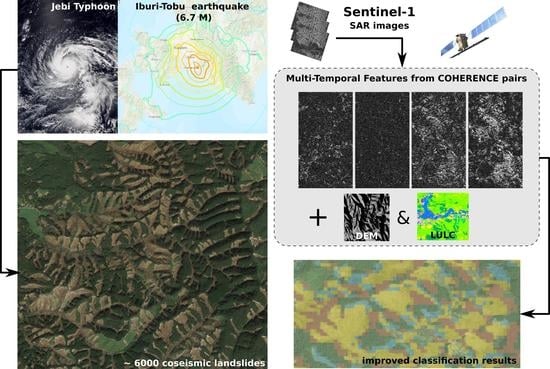
Do We Need a Higher Resolution? Case Study: Sentinel-1-Based Change Detection of the 2018 Hokkaido Landslides, Japan

 ,
,  , ,
, ,  and
and
Abstract
:
1. Introduction
2. Material and Methods
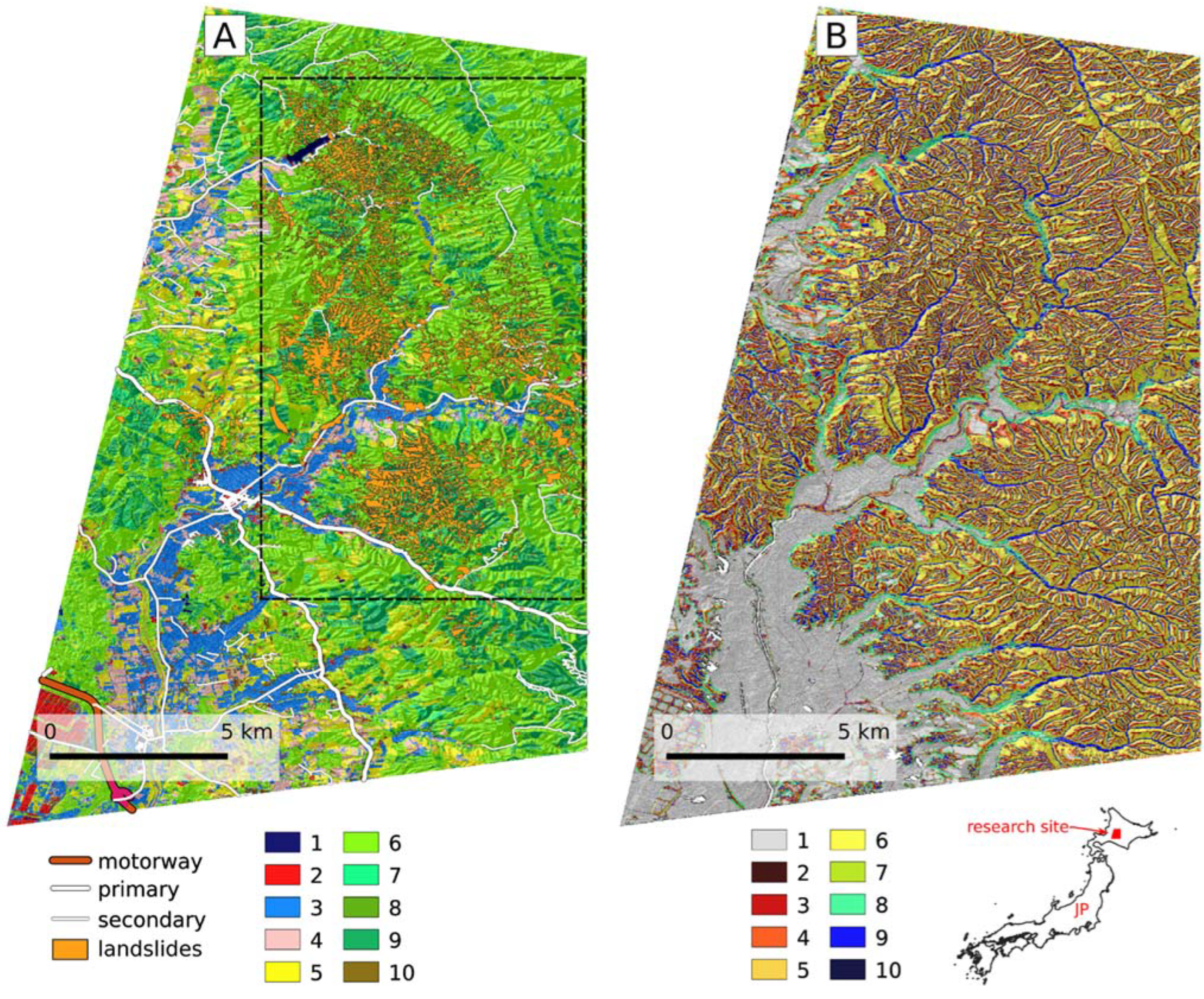
2.1. Site Description
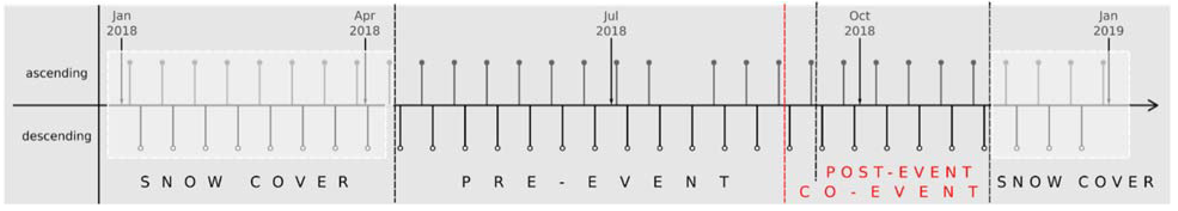
2.2. Data
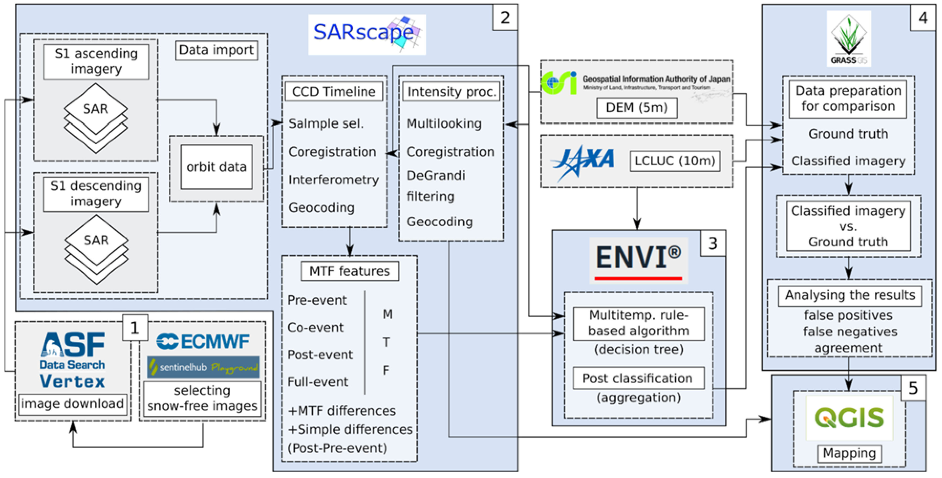
2.3. Methods
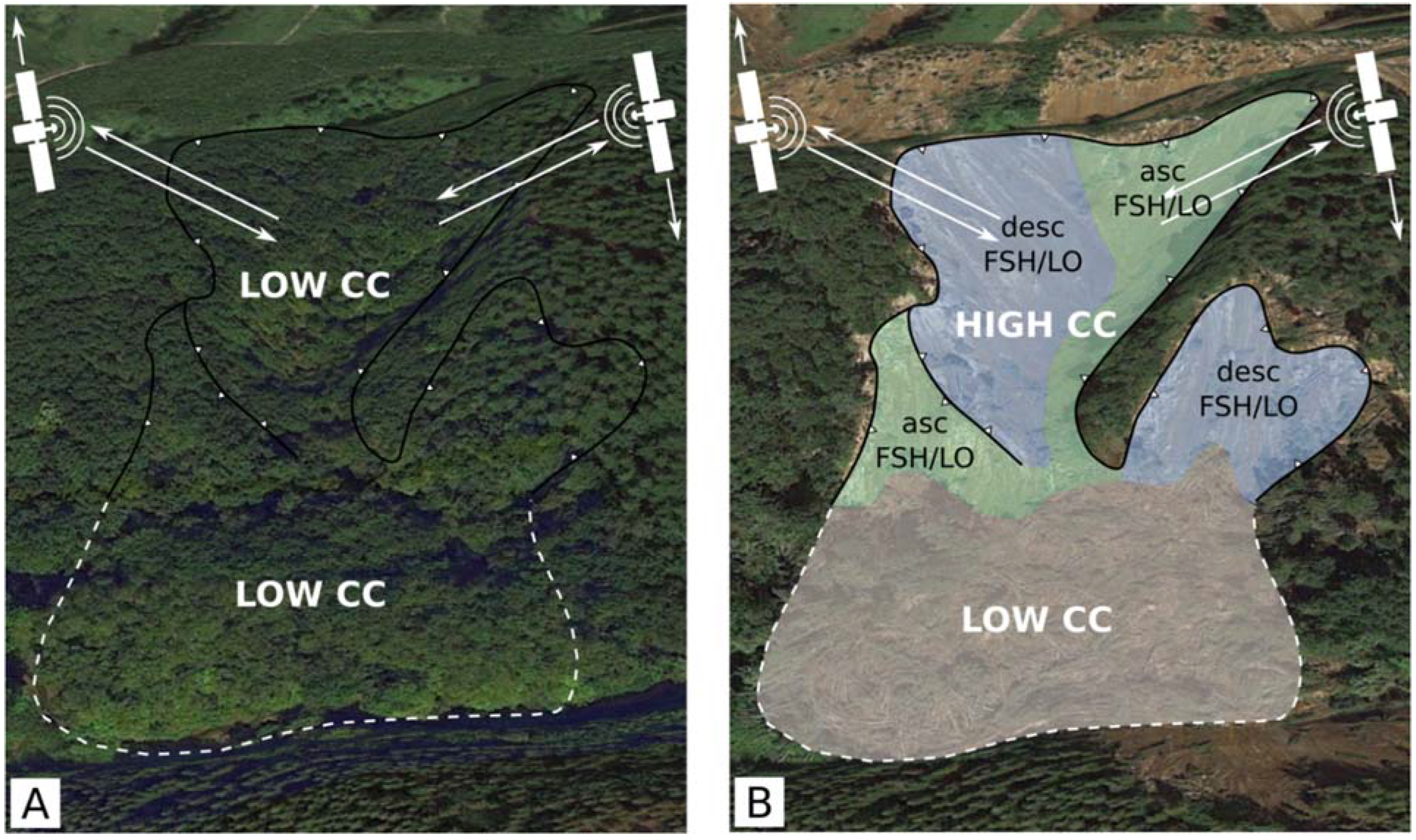
2.3.1. A Priori Considerations
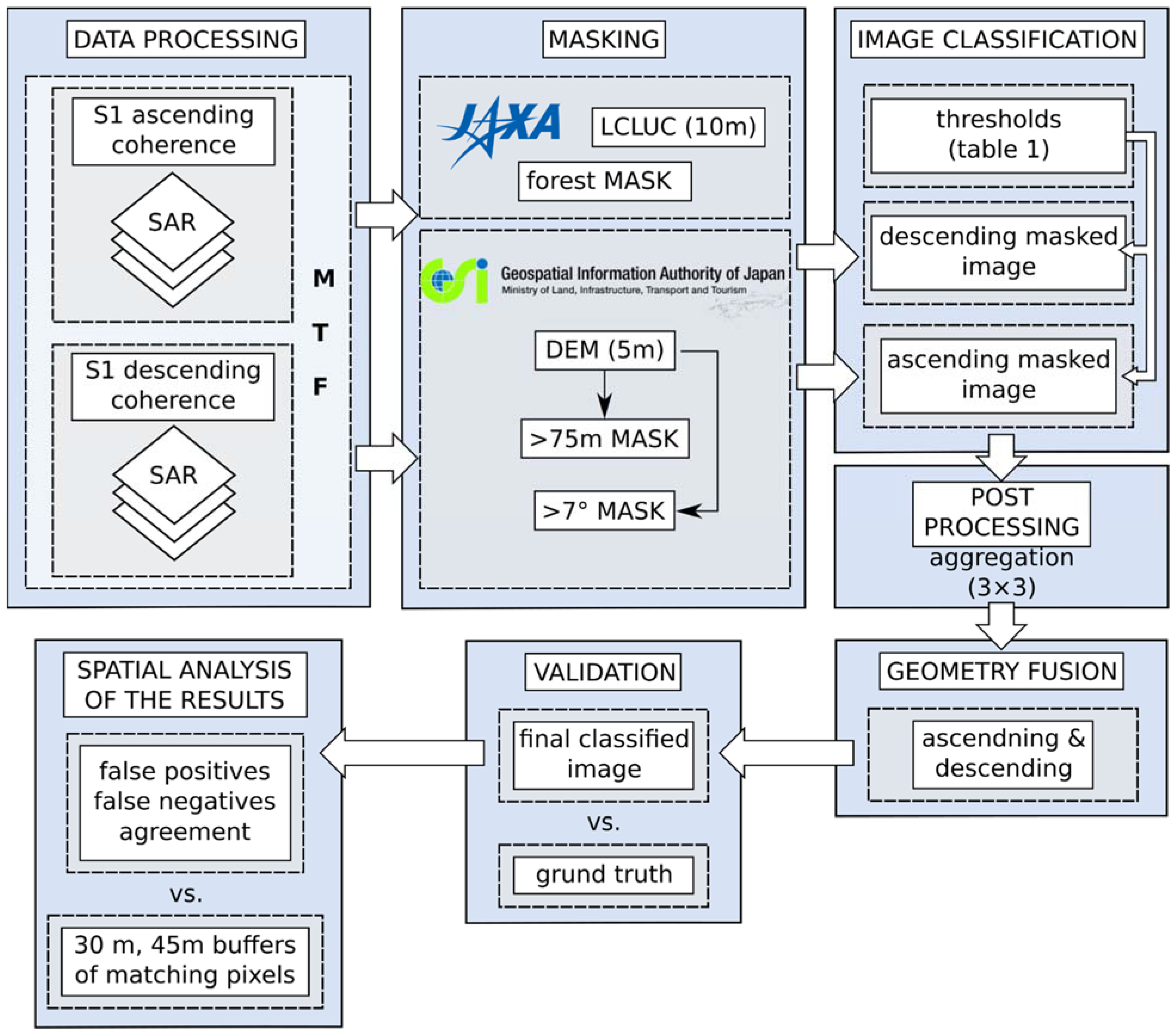
2.3.2. Image Processing
2.3.3. Image Classification and Post-Processing
3. Results
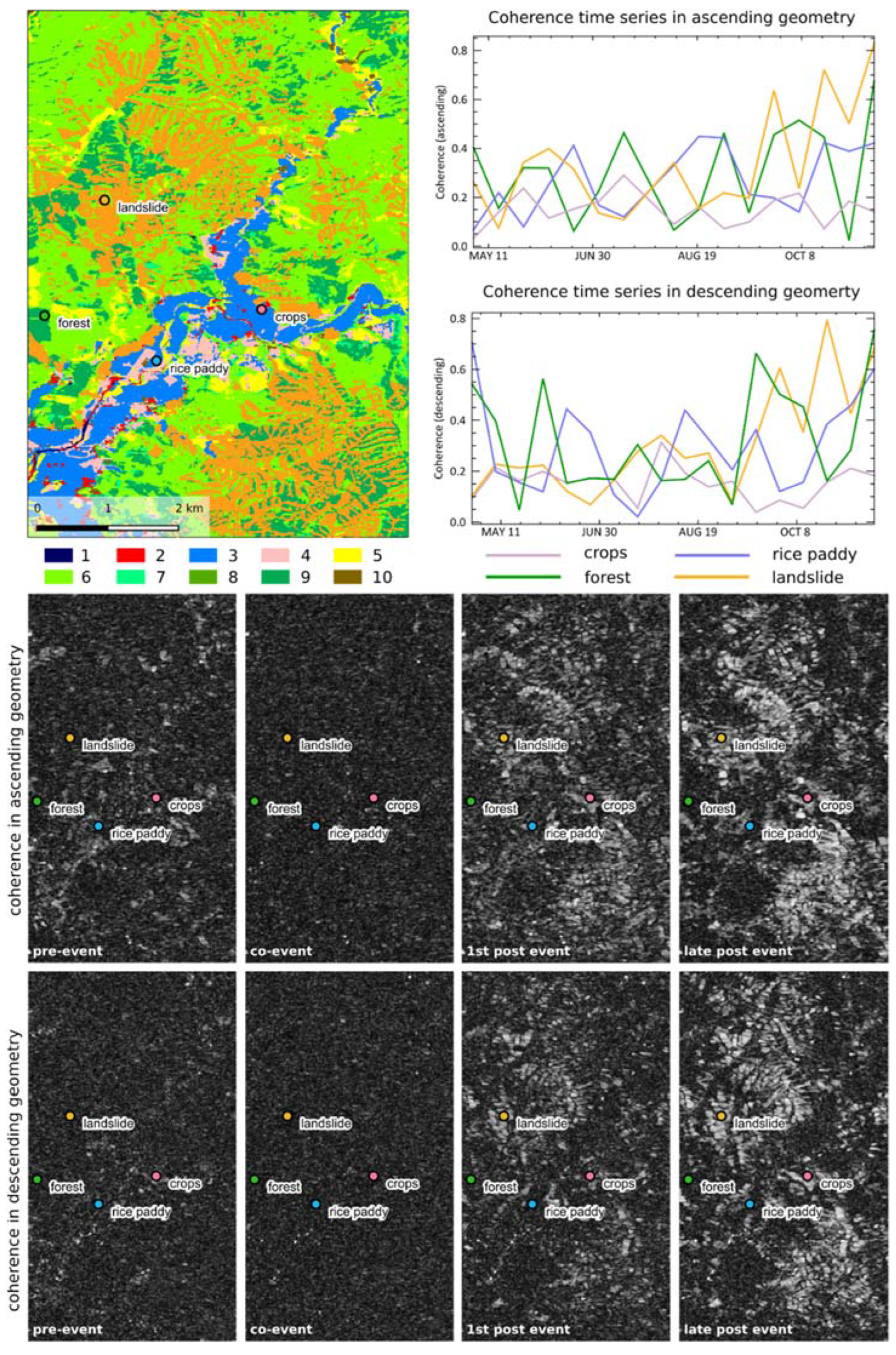
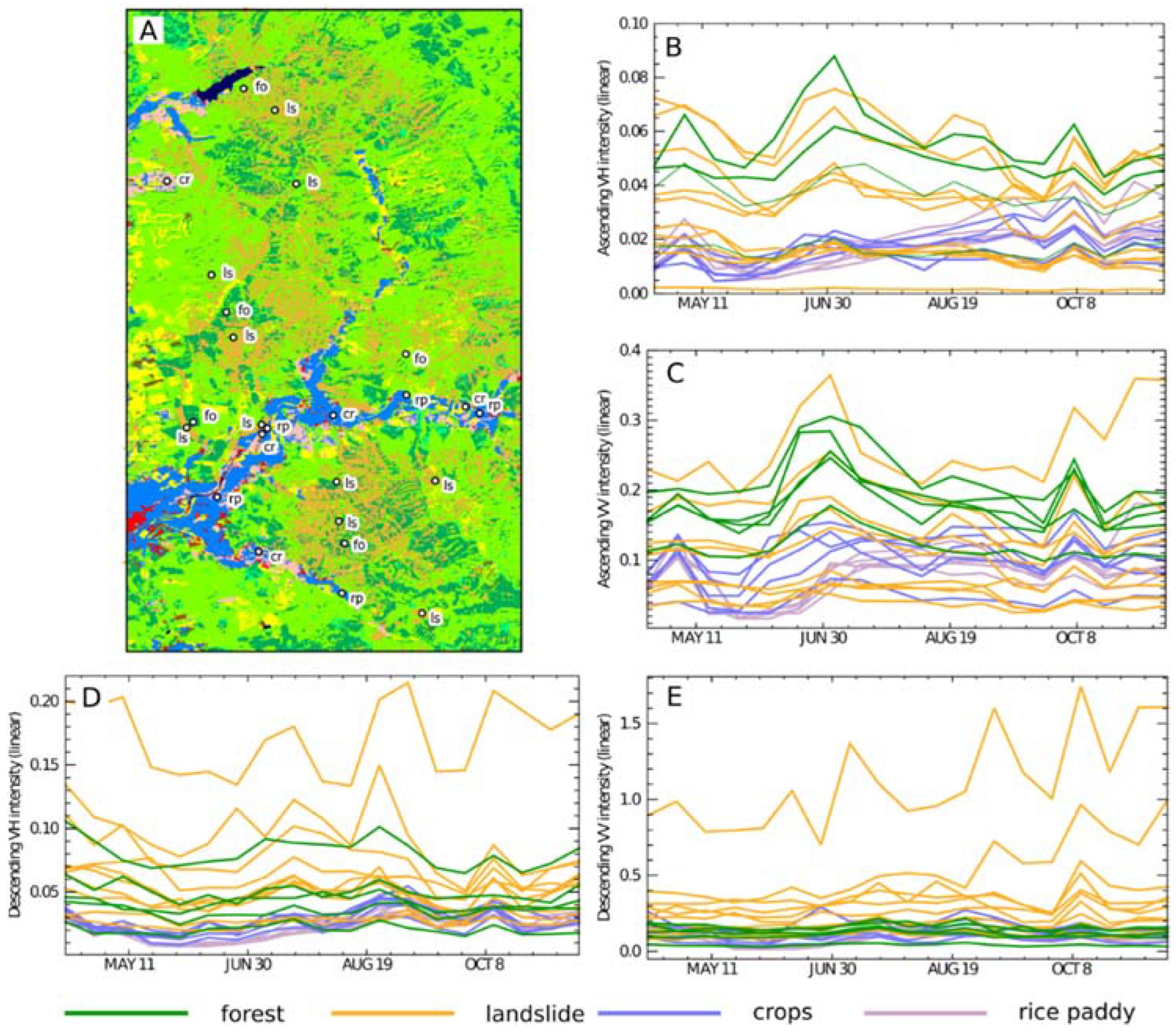
3.1. Temporal Changes in Intensity
3.2. Temporal Changes of the Coherence over the Study Site
3.3. Image Classification Results
4. Discussion
5. Conclusions
Author Contributions
Funding
Institutional Review Board Statement
Data Availability Statement
Acknowledgments
Conflicts of Interest
List of Abbreviations
| APS | Atmospheric Phase Screen |
| CCD | Coherence Change Detection |
| DEM | Digital Elevation Model |
| DInSAR | Differential Synthetic Aperture Radar Interferometry |
| ECMWF | European Centre for Medium-Range Weather Forecasts |
| ESA | European Space Agency |
| FSH | Foreshortening |
| GB-InSAR | Ground-based synthetic aperture radar interferometry |
| GIS | Geogprahic Insformation System |
| GPS | Global Positioning System |
| GSI | Geospatial Information Authority of Japan |
| InSAR | Synthetic Aperture Radar Interferometry |
| LIDAR | Light Detection and Ranging |
| LO | Layover |
| LULC | Land Use and Land Cover |
| MTF | Multitemporal features |
| NASA | National Aeronautics and Space Administration |
| PS | Permanent Scatterers |
| PSI | Persistent Scatterers |
| SAR | Synthetic Aperture Radar |
| SBAS | Small-Baseline Subsets |
| SLC | Single Look Complex |
| TLS | Terrestrial laser scanning |
References
- Kirschbaum, D.B.; Adler, R.F.; Hong, Y.; Lerner-Lam, A. Evaluation of a preliminary satellite-based landslide hazard algorithm using global landslide inventories. Nat. Hazards Earth Syst. Sci. 2009, 9, 673–686. [Google Scholar] [CrossRef] [Green Version]
- Kirschbaum, D.; Adler, R.; Hong, Y.; Kumar, S.; Peters-Lidard, C.; Lerner-Lam, A. Advances in landslide nowcasting: Evaluation of a global and regional modeling approach. Environ. Earth Sci. 2012, 66, 1683–1696. [Google Scholar] [CrossRef] [Green Version]
- Petley, D.; Dunning, S.A.; Rosser, N.J. The analysis of global landslide risk through the creation of a database of worldwide landslide fatalities. In Landslide Risk Management; Hungr, O., Fell, R., Couture, R., Eberhardt, E., Eds.; CRC Press: Cambridge, UK, 2005; pp. 367–374. ISBN 9780429151354. [Google Scholar]
- Petley, D. Global patterns of loss of life from landslides. Geology 2012, 40, 927–930. [Google Scholar] [CrossRef]
- Haque, U.; Blum, P.; da Silva, P.F.; Andersen, P.; Pilz, J.; Chalov, S.R.; Malet, J.P.; Auflič, M.J.; Andres, N.; Poyiadji, E.; et al. Fatal landslides in Europe. Landslides 2016, 13, 1545–1554. [Google Scholar] [CrossRef]
- Lin, Q.; Wang, Y. Spatial and temporal analysis of a fatal landslide inventory in China from 1950 to 2016. Landslides 2018, 15, 2357–2372. [Google Scholar] [CrossRef]
- Gokceoglu, C.; Sezer, E.A. statistical assessment on international landslide literature (1945–2008). Landslides 2009, 6, 345–351. [Google Scholar] [CrossRef]
- Guzzetti, F.; Carrara, A.; Cardinali, M.; Reichenbach, P. Landslide hazard evaluation: A review of current techniques and their application in a multi-scale study, Central Italy. Geomorphology 1999, 31, 181–216. [Google Scholar] [CrossRef]
- Guzzetti, F.; Reichenbach, P.; Cardinali, M.; Galli, M.; Ardizzone, F. Probabilistic landslide hazard assessment at the basin scale. Geomorphology 2005, 72, 272–299. [Google Scholar] [CrossRef]
- Uhlemann, S.; Smith, A.; Chambres, J.; Dixon, N.; Dijkstra, T.; Haslan, E.; Meldrum, P.; Merritt, A.; Gunn, D.; Mackay, J. Assessment of ground-based monitoring techniques applied to landslide investigations. Geomorphology 2016, 253, 438–451. [Google Scholar] [CrossRef] [Green Version]
- Van Westen, C.J.; Castellanos, E.; Kuriakose, S.L. Spatial data for landslide susceptibility, hazards and vulnerability assessment: An overview. Eng. Geol. 2008, 102, 112–131. [Google Scholar] [CrossRef]
- Carlà, T.; Macciotta, R.; Hendry, M.; Martin, D.; Edwards, T.; Evans, T.; Farina, P.; Intrieri, E.; Casagli, N. Displacement of a landslide retaining wall and application of an enhanced failure forecasting approach. Landslides 2018, 15, 489–505. [Google Scholar] [CrossRef] [Green Version]
- Garcia, A.; Hordt, A.; Fabian, M. Landslide monitoring with high resolution tilt measurements at the Dollendorfer Hardt landslide, Germany. Geomorphology 2010, 120, 16–25. [Google Scholar] [CrossRef]
- Guerriero, L.; Guadagno, F.M.; Revellino, P. Estimation of earth-slide displacement from GPS-based surface-structure geometry reconstruction. Landslides 2018, 16, 425–430. [Google Scholar] [CrossRef]
- Guzzetti, F.; Mondini, A.C.; Cardinali, M.; Fiorucci, F.; Santangelo, M.; Chang, K.T. Landslide inventory maps: New tools for an old problem. Earth-Sci. Rev. 2012, 112, 42–66. [Google Scholar] [CrossRef] [Green Version]
- Huang, R.; Jiang, L.; Shen, X.; Dong, Z.; Zhou, Q.; Yang, B.; Wang, H. An efficient method of monitoring slow- moving landslides with long-range terrestrial laser scanning: A case study of the Dashu landslide in the Three Gorges Reservoir Region, China. Landslides 2018, 16, 839–855. [Google Scholar] [CrossRef]
- Casagli, N.; Catani, F.; Del Ventisette, C.; Luzi, G. Ground-based Interferometry for landslide monitoring. In Landslide Dynamics: ISRD-ICL Landslide Interactive Teaching Tools, Volume 1 Fundamentals, Mapping and Monitoring; Sassa, K., Guzzetti, F., Yamagishi, H., Abranas, Z., Casagli, N., McSaveney, M., Eds.; Springer: Cham, Switzerland, 2015. [Google Scholar] [CrossRef]
- Savvaidis, P.D. Existing landslide monitoring systems and techniques. In From Stars to Earth and Culture, in Honor of the Memory of Professor Alexandros Tsioumis; The Aristotle University of Thessaloniki: Thessaloniki, Greece, 2003; pp. 242–258. [Google Scholar]
- Maček, M.; Petkovšek, A.; Bojan, M.; Mikoš, M. Landslide Monitoring Techniques Database. In World Landslide Forum 3, Bejing, China. Volume: Landslide Science for a Safer Geoenvironment, Vol. 1: The International Programme on Landslides; Springer: Cham, Switzerland, 2014; pp. 193–197. [Google Scholar] [CrossRef]
- Angeli, M.G.; Pasuto, A.; Silvano, S. A critical review of landslide monitoring experiences. Eng. Geol. 2000, 55, 133–147. [Google Scholar] [CrossRef]
- Liu, S.; Wang, Z. Choice of surveying methods for landslides monitoring. In Landslides and Engineered Slopes; Chen, Z., Zhang, J.-M., Ho, K., Wu, F.-Q., Eds.; Taylor and Francis Group: London, UK, 2008; pp. 1211–1216. ISBN 978-0-415-41196-7. [Google Scholar]
- Arbanas, S.M.; Arbanas, Z. Landslide mapping and monitoring: Review of conventional and advanced techniques. In Proceedings of the 4th Symposium of Macedonian Association for Geotechnics, Skopje, North Macedonia, 25–28 June 2014; pp. 57–72. [Google Scholar]
- Jaboyedoff, M.; Oppikofer, T.; Abellán, A.; Derron, M.H.; Loye, A.; Metzger, R.; Pedrazzini, A. Use of LIDAR in landslide investigations: A review. Nat. Hazards 2012, 61, 5–28. [Google Scholar] [CrossRef] [Green Version]
- Zhao, C.; Lu, Z. Remote Sensing of Landslides—A Review. Remote Sens. 2018, 10, 279. [Google Scholar] [CrossRef] [Green Version]
- Kovács, I.P.; Bugya, T.; Czigány, S.; Defilippi, M.; Dobre, B.; Fábián, S.Á.; Lóczy, D.; Riccardi, P.; Ronczyk, L.; Pasquali, P. Monitoring landslides using C-band interferometry. A case study: Dunaszekcső Landslide, Southern Transdanubia, Hungary. Studia Geomorphol. Carpatho-Balc. 2018, 51–52, 87–105. [Google Scholar]
- Kovács, I.P.; Bugya, T.; Czigány, S.; Defilippi, M.; Lóczy, D.; Riccardi, P.; Ronczyk, L.; Pasquali, P. How to avoid false interpretations of Sentinel-1A TOPSAR interferometric data in landslide mapping? A case study: Recent landslides in Transdanubia, Hungary. Nat. Hazards 2018, 96, 693–712. [Google Scholar] [CrossRef] [Green Version]
- Glade, T.; Anderson, M.; Crozier, M.J. Landslide Hazard and Risk; John Wiley & Sons Ltd.: Chichester, UK, 2005; p. 802. [Google Scholar]
- Tofani, V.; Raspini, F.; Catani, F.; Casagli, N. Persistent Scatterer Interferometry (PSI) technique for land-slide characterization and monitoring. Remote Sens. 2013, 5, 1045–1065. [Google Scholar] [CrossRef] [Green Version]
- Pecoraro, G.; Calvello, M.; Piciullo, L. Monitoring strategies for local landslide early warning systems. Landslides 2018, 16, 213–231. [Google Scholar] [CrossRef]
- Chae, B.G.; Park, H.J.; Catani, F.; Simoni, A.; Berti, M. Landslide prediction, monitoring and early warning: A concise review of state-of-the-art. Geosci. J. 2017, 21, 1033–1070. [Google Scholar] [CrossRef]
- Pardeshi, S.D.; Autade, S.E.; Pardeshi, S.S. Landslide hazard assessment: Recent trends and techniques. SpringerPlus 2013, 2, 523. [Google Scholar] [CrossRef] [Green Version]
- Corominas, J.; van Westen, C.J.; Frattini, P.; Cascini, L.; Malet, J.P.; Fotopoulou, S.; Catani, S.; Van Den Eeckhaut, M.; Mavrouli, O.; Agliardi, F.; et al. Recommendations for the quantitative analysis of landslide risk. Bull. Eng. Geol. Environ. 2014, 73, 209–263. [Google Scholar] [CrossRef]
- Reichenbach, P.; Rossi, M.; Malamud, B.D.; Mihir, M.; Guzzetti, F. A review of statistically-based landslide susceptibility models. Earth-Sci. Rev. 2018, 180, 60–91. [Google Scholar] [CrossRef]
- Hein, A. Processing of SAR Data. Fundamentals, Signal Processing, Interferometry; Springer: Berlin/Heidelberg, Germany, 2004; p. 291. [Google Scholar] [CrossRef]
- Barra, A.; Monserrat, O.; Mazzanti, P.; Esposito, C.; Crosetto, M.; Mugnozza, G.S. First insights on the potential of Sentinel-1 for landslides detection. Geomat. Nat. Hazards Risk 2016, 7, 1874–1883. [Google Scholar] [CrossRef] [Green Version]
- Gariano, S.F.; Guzzetti, F. Landslides in a changing climate. Earth-Sci. Rev. 2016, 162, 227–252. [Google Scholar] [CrossRef] [Green Version]
- Sowter, A.; Bin Che Amat, M.; Cigna, F.; Marsh, S.; Athab, A.; Alshammari, L. Mexico City land subsidence in 2014–2015 with Sentinel-1 IW TOPS: Results using Intermittent SBAS (ISBAS) technique. Int. J. Appl. Earth Obs. Geoinf. 2016, 52, 230–242. [Google Scholar] [CrossRef]
- Pourghasemi, H.R.; Teimoori Yansari, Z.; Panagos, P.; Pradhan, B. Analysis and evaluation of landslide susceptibility: A review on articles published during 2005–2016 (periods of 2005–2012 and 2013–2016). Arab. J. Geosci. 2018, 11, 193. [Google Scholar] [CrossRef]
- Lee, S. Current and Future Status of GIS-based Landslide Susceptibility Mapping: A Literature Review. Korean J. Remote Sens. 2019, 35, 179–193. [Google Scholar] [CrossRef]
- Ferretti, A.; Prati, C.; Rocca, F. Permanent scatterers in SAR interferometry. Trans. Geosci. Remote Sens. 2001, 39, 8–20. [Google Scholar] [CrossRef]
- Ferretti, A. Satellite InSAR Data. Reservoir Monitoring from Space; EAGE Publications: Houten, The Netherlands, 2014; p. 160. [Google Scholar]
- Pasquali, P.; Cantone, A.; Riccardi, P.; Defilippi, M.; Ogushi, F.; Gagliano, S.; Tamura, M. Mapping of ground deformations with interferometric stacking techniques. In Land Applications of Radar Remote Sensing; Holecz, F., Pasquali, P., Milisavljevic, N., Eds.; InTechOpen: London, UK, 2014; pp. 231–258. [Google Scholar] [CrossRef] [Green Version]
- Piacentini, D.; Devoto, S.; Mantovani, M.; Pasuto, A.; Prampolini, M.; Soldati, M. Landslide susceptibility modeling assisted by Persistent Scatterers Interferometry (PSI): An example from the northwestern coast of Malta. Nat. Hazards 2015, 78, 681–697. [Google Scholar] [CrossRef] [Green Version]
- Wasowski, J.; Bovenga, F. Remote sensing of landslide motion with emphasis on satellite multitemporal interferometry applications: An overview. In Landslide Hazards, Risk, and Disasters; Davies, T., Ed.; Elsevier: Amsterdam, The Netherlands, 2015; pp. 345–403. [Google Scholar]
- Wasowski, J.; Bovenga, F. Investigating landslides and unstable slopes with satellite Multi Temporal Interferometry: Current issues and future perspectives. Eng. Geol. 2014, 174, 103–138. [Google Scholar] [CrossRef]
- Rott, H.; Nagler, T. The contribution of radar interferometry to assessment of landslide hazards. Adv. Space Res. 2006, 37, 710–719. [Google Scholar] [CrossRef]
- Preiss, M.; Stacy, J.S. Coherent Change Detection: Theoretical Description and Experimental Results; Defence Science and Technology Organisation, Intelligence, Surveillance and Reconnaissance Division: Edinburgh, Australia, 2006; p. 104. [Google Scholar]
- Dwyer, E.; Monaco, S.; Pasquali, P. An operational forest mapping tool using spaceborne SAR data. In Proceedings of the ERS-ENVISAT Symposium, Gothenburg, Sweden, 16–20 October 2000. [Google Scholar]
- Holecz, F.; Barbieri, M.; Cantone, A.; Pasquali, P.; Monaco, S. Synergetic Use of ALOS PALSAR, ENVISAT ASAR and Landsat TM/ETM+ Data for Land Cover and Change Mapping. In JAXA Kyoto and Carbon Initiative; Japan Aerospace Exploration Agency, Earth Observation Research Cente: Tokyo, Japan, 2009; p. 6. [Google Scholar]
- Kellndorfer, J.; Cartus, O.; Bishop, J.; Walker, W.; Holecz, F. Large scale mapping of forests and land cover with synthetic aperture radar data. In Land Applications of Radar Remote Sensing; Closson, D., Holecz, F., Pasquali, P., Milisavljevic, N., Eds.; InTechOpen: London, UK, 2014; pp. 59–94. [Google Scholar] [CrossRef] [Green Version]
- Milisavljević, N.; Collivignarelli, F.; Holecz, F. Estimation of Cultivated Areas Using Multi-Temporal SAR Data. In Land Applications of Radar Remote Sensing; Closson, D., Holecz, F., Pasquali, P., Milisavljevic, N., Eds.; InTechOpen: London, UK, 2014; pp. 95–120. [Google Scholar] [CrossRef] [Green Version]
- Milisavljević, N.; Closson, D.; Block, I. Detecting human-induced changes using coherent change detection in SAR images. In Proceedings of the ISPRS TC VII Symposium, Vienna, Austria, 5–7 July 2010; Wagner, W., Székely, B., Eds.; Vienna University of Technology: Vienna, Austria, 2010; Volume 38, Part 7B, pp. 387–394. [Google Scholar]
- Liu, J.G.; Mason, P.; Hilton, F.; Lee, H. Detection of Rapid Erosion in SE Spain: A GIS Approach Based on ERS SAR Coherence Imagery. Photogramm. Eng. Remote Sens. 2004, 70, 1179–1185. [Google Scholar] [CrossRef]
- Nico, G.; Pappalepore, M.; Pasquariello, G.; Refice, A.; Samarelli, S. Comparison of SAR amplitude vs. coherence flood detection methods-a GIS application. Int. J. Remote Sens. 2000, 21, 1619–1631. [Google Scholar] [CrossRef]
- Atzori, S.; Tolomei, C.; Antonioli, A.; Merryman Boncori, J.P.; Bannister, S.; Trasatti, E.; Pasquali, P.; Salvi, S. The 2010–2011 Canterbury, New Zealand seismic sequence: Multiple source analysis from InSAR data and modeling. J. Geophys. Res. (Solid Earth) 2012, 117, 1857–1861. [Google Scholar] [CrossRef]
- Washaya, P.; Balz, T. SAR coherence change detection of urban areas affected by disasters using Sentinel-1 imagery. Int. Arch. Photogramm. Remote Sens. Spat. Inf. Sci. 2018, 42, 1857–1861. [Google Scholar] [CrossRef] [Green Version]
- Washaya, P.; Balz, T.; Mohamadi, B. Coherence Change-Detection with Sentinel-1 for Natural and Anthropogenic Disaster Monitoring in Urban Areas. Remote Sens. 2018, 10, 1026. [Google Scholar] [CrossRef] [Green Version]
- Tessari, G.; Floris, M.; Pasquali, P. Phase and amplitude analyses of SAR data for landslide detection and monitoring in non-urban areas located in the North-Eastern Italian pre-Alps. Environ. Earth Sci. 2017, 76, 85. [Google Scholar] [CrossRef]
- Osmanoğlu, B.; Sunar, F.; Wdowinski, S.; Cabral-Cano, E. Time series analysis of InSAR data: Methods and trends. ISPRS J. Photogramm. Remote Sens. 2015, 115, 90–102. [Google Scholar] [CrossRef]
- Bovenga, F.; Pasquariello, G.; Refice, A. Statistically-Based Trend Analysis of MTInSAR Displacement Time Series. Remote Sens. 2021, 13, 2302. [Google Scholar] [CrossRef]
- Ghaderpour, E. JUST: MATLAB and python software for change detection and time series analysis. GPS Solut. 2021, 25, 85. [Google Scholar] [CrossRef]
- Plank, S. Rapid damage assessment by means of multi-temporal SAR—A comprehensive review and outlook to Sentinel-1. Remote Sens. 2014, 6, 4870–4906. [Google Scholar] [CrossRef] [Green Version]
- Ito, Y.; Hosokawa, M.; Lee, H.; Liu, J.G. Extraction of damaged regions using SAR data and neural networks. International Archives of Photogrammetry. Remote Sens. 2000, 33, 156–163. [Google Scholar]
- Ito, Y.; Hosokawa, M. Damage Estimation Model Using Temporal Coherence Ratio. In Proceedings of the IEEE IGARSS, Toronto, ON, Canada, 24–28 June 2002; pp. 2859–2861. [Google Scholar]
- Yonezawa, C.; Tomiyama, N.; Takeuchi, S. Urban Damage Detection Using Decorrelation of SAR Interferometric Data. In Proceedings of the IEEE IGARSS, Toronto, ON, Canada, 24–28 June 2002; pp. 2051–2053. [Google Scholar]
- Hoffmann, J. Mapping damage during the Bam (Iran) earthquake using interferometric coherence. Int. J. Remote Sens. 2007, 28, 1199–1216. [Google Scholar] [CrossRef]
- Mansouri, B.; Shinozuka, M.; Huyck, C.; Houshmand, B. Earthquake-induced change detection in the 2003 Bam, Iran, earthquake by complex analysis using Envisat ASAR data. Earthq. Spectra 2005, 21, 275–284. [Google Scholar] [CrossRef]
- Matsuoka, M.; Yamazaki, F. Building damage mapping of the 2003 Bam, Iran, earthquake using Envisat/ASAR intensity imagery. Earthq. Spectra 2005, 21, 285–294. [Google Scholar] [CrossRef]
- Chini, M.; Bignami, C.; Stramondo, S.; Pierdicca, N. Uplift and subsidence due to the 26 December 2004 Indonesian earthquake detected by SAR data. Int. J. Remote Sens. 2008, 29, 3891–3910. [Google Scholar] [CrossRef]
- Matsuoka, M.; Yamazaki, F. Application of the Damage Detection Method Using SAR Intensity Images to Recent Earthquakes. In Proceedings of the IEEE IGARSS, Toronto, ON, Canada, 24–28 June 2002; pp. 2042–2044. [Google Scholar]
- Yonezawa, C.; Takeuchi, S. Decorrelation of SAR data by urban damages caused by the 1995 Hyogoken-nanbu earthquake. Int. J. Remote Sens. 2001, 22, 1585–1600. [Google Scholar] [CrossRef]
- Matsuoka, M.; Yamazaki, F. Characteristics of Satellite SAR Images in the Areas Damaged by Earthquakes. In Proceedings of the IEEE IGARSS, Honolulu, HY, USA, 24–28 July 2000; pp. 2693–2696. [Google Scholar]
- Aimaiti, Y.; Liu, W.; Yamazaki, F.; Maruyama, Y. Earthquake-induced landslide mapping for the 2018 Hokkaido Eastern Iburi Earthquake using PALSAR-2 data. Remote Sens. 2019, 11, 2351. [Google Scholar] [CrossRef] [Green Version]
- Fujiwara, S.; Nakano, T.; Morishita, Y.; Kobayashi, T.; Yarai, H.; Une, H.; Hayashi, K. Detection and interpretation of local surface deformation from the 2018 Hokkaido Eastern Iburi Earthquake using ALOS-2 SAR data. Earth Planets Space 2019, 71, 64. [Google Scholar] [CrossRef]
- Jung, J.; Yun, S. Evaluation of Coherent and Incoherent Landslide Detection Methods Based on Synthetic Aperture Radar for Rapid Response: A Case Study for the 2018 Hokkaido Landslides. Remote Sens. 2020, 12, 265. [Google Scholar] [CrossRef] [Green Version]
- Zhang, S.; Li, R.; Wang, F.; Iio, A. Characteristics of landslides triggered by the 2018 Hokkaido Eastern Iburi earthquake, Northern Japan. Landslides 2019, 16, 1691–1708. [Google Scholar] [CrossRef]
- Yamagishi, H.; Yamazaki, F. Landslides by the 2018 Hokkaido Iburi-Tobu Earthquake on September 6. Landslides 2018, 15, 2521–2524. [Google Scholar] [CrossRef] [Green Version]
- Hirose, W.; Kawakami, G.; Kase, Y.; Ishimaru, S.; Koshimizu, K.; Koyasu, H.; Takahashi, R. Preliminary report of slope movements at Atsuma Town and its surrounding areas caused by the 2018 Hokkaido Eastern Iburi Earthquake. Rep. Local Indep. Adm. Agency Hokkaido Res. Organ. 2018, 90, 33–44. [Google Scholar]
- Wang, F.; Fan, X.; Yunus, A.P.; Subramanian, S.S.; Alonso-Rodriguez, A.; Dai, L.; Xu, Q.; Huang, R. Coseismic landslides triggered by the 2018 Hokkaido, Japan (Mw 6.6), earthquake: Spatial distribution, controlling factors, and possible failure mechanism. Landslides 2019, 16, 1551–1566. [Google Scholar] [CrossRef]
- Tajika, J.; Ohtsu, S.; Inui, T. Interior structure and sliding process of landslide body composed of stratified pyroclastic fall deposits at the Apporo 1 archaeological site, southeastern margin of the Ishikari Lowland, Hokkaido, North Japan. J. Geol. Soc. Jpn. 2016, 122, 23–35. [Google Scholar] [CrossRef] [Green Version]
- Kameda, J.; Kamiya, H.; Masumoto, H.; Morisaki, T.; Hiratsuka, T.; Inaoi, C. Fluidized landslides triggered by the liquefaction of subsurface volcanic deposits during the 2018 Iburi-Tobu earthquake, Hokkaido. Sci. Rep. 2019, 9, 13119. [Google Scholar] [CrossRef]
- Hashimoto, S.; Tadono, T.; Onosato, M.; Hori, M.; Shiomi, K. A New Method to Derive Precise Land-use and Land-cover Maps Using Multi-temporal Optical Data. J. Remote Sens. Soc. Jpn. 2014, 34, 102–112. [Google Scholar]
- Jasiewicz, J.; Stepinski, T. Geomorphons—A pattern recognition approach to classification and mapping of landforms. Geomorphology 2013, 182, 147–156. [Google Scholar] [CrossRef]
- Alaska Satellite Facility Server. Available online: https://search.asf.alaska.edu/#/ (accessed on 3 March 2022).
- European Centre for Medium-Range Weather Forecasts (ECMWF) Data Dissemination Service. Available online: https://apps.ecmwf.int/datasets/data/interim-full-daily/levtype=sfc/ (accessed on 3 March 2022).
- Sentinel Playground. Available online: https://www.sentinel-hub.com/explore/sentinelplayground/ (accessed on 3 March 2022).
- Geospatial Information Authority of Japan, AW3D Standard. Available online: https://www.aw3d.jp/en/products/standard/ (accessed on 3 March 2022).
- ALOS Research and Application Project, High-Resolution Land Use and Land Cover Map Products. Available online: https://www.eorc.jaxa.jp/ALOS/en/dataset/lulc_e.htm (accessed on 3 March 2022).
- Characteristics of Lanslides Triggered by the 2018 Hokkaido Eastern Iburi Earthquake, North Japan. Available online: https://zenodo.org/record/2577300#.YiInDOjMJhE (accessed on 3 March 2022).
- Gutman, G.; Byrnes, R.; Masek, J.; Covington, S.; Justice, C.; Franks, S.; Headley, R. Towards monitoring land cover and land use changes at a global scale: The Global Land Survey 2005. Photogramm. Eng. Remote Sens. 2008, 74, 6–10. [Google Scholar]
- Bouaraba, A.; Milisavljević, N.; Acheroy, M.; Closson, D. Change Detection and Classification Using HighResolution SAR Interferometry. In Land Applications of Radar Remote Sensing; Closson, D., Holecz, F., Pasquali, P., Milisavljevic, N., Eds.; InTechOpen: London, UK, 2014; pp. 149–163. [Google Scholar] [CrossRef] [Green Version]
- Closson, D.; Milisavljevic, N. InSAR Coherence and Intensity Changes Detection. In Mine Action—The Research Experience of the Royal Military Academy of Belgium; Beumier, C., Closson, D., Lacroix, V., Milisavljevic, N., Yvinec, Y., Eds.; InTechOpen: London, UK, 2014; pp. 155–176. [Google Scholar] [CrossRef] [Green Version]
- De Grandi, G.F.; Leysen, M.; Lee, J.S.; Schuler, D. Radar reflectivity estimation using multiple SAR scenes of the same target: Technique and applications. In Proceedings of the IGARSS’97, IEEE International Geoscience and Remote Sensing Symposium Proceedings, Remote Sensing—A Scientific Vision for Sustainable Development, Singapore, 3–8 August 1997; Volume 2, pp. 1047–1050. [Google Scholar] [CrossRef]
- Campos-Taberner, M.; García-Haro, F.J.; Camps-Valls, G.; Grau-Muedra, G.; Nutini, F.; Busetto, L.; Katsantonis, D.; Stavrakoudis, D.; Minakou, C.; Gatti, L.; et al. Exploitation of SAR and Optical Sentinel Data to Detect Rice Crop and Estimate Seasonal Dynamics of Leaf Area Index. Remote Sens. 2017, 9, 248. [Google Scholar] [CrossRef] [Green Version]
- Olofsson, P.; Foody, G.M.; Herold, M.; Stehmand, S.V.; Woodcock, C.E.; Wulder, M.A. Good practices for estimating area and assessing accuracy of land change. Remote Sens. Environ. 2014, 148, 42–57. [Google Scholar] [CrossRef]
- ESA WorldCover—Worldwide Land Cover Mapping. Available online: https://esa-worldcover.org/en (accessed on 3 March 2022).
- ALOS Research and Application Project. Available online: https://www.eorc.jaxa.jp/ALOS/en/index_e.htm (accessed on 3 March 2022).
- The European Space Agency—Sentinel Mission Guide. Available online: https://sentinel.esa.int/web/sentinel/missions/sentinel-1 (accessed on 3 March 2022).


| Event-Type | Calculated Feature | Ascending Threshold | Descending Threshold | |
|---|---|---|---|---|
| MTF | Co-event | mean | >0.3 | >0.3 |
| maximum | >0.45 | >0.45 | ||
| span difference | >0.4 | >0.4 | ||
| Post-event | minimum | >0.175 | >0.175 | |
| mean | >0.3 | >0.35 | ||
| maximum | >0.45 | >0.5 | ||
| Full event | maximum | >0.45 | >0.55 | |
| mean | >0.21 | >0.25 | ||
| standard deviation | >0.12 | >0.125 | ||
| MTF differences | Co-event Pre-event difference | mean | >0.1 | >0.1 |
| maximum | >0.15 | >0.175 | ||
| standard deviation | >0.075 | >0.075 | ||
| Post-event Pre-event difference | minimum | >0.1 | >0.1 | |
| mean | >0.14 | >0.125 | ||
| maximum | >0.14 | >0.15 | ||
| Post-Pre event coherence difference | >0.2 | >0.2 | ||
| Geometry | Feature Type | Event Type | False Negative % | False Positive % | Match % |
|---|---|---|---|---|---|
| Ascending | MTF | co | 47.843 | 5.7192 | 52.1569 |
| post | 51.2658 | 6.5564 | 48.7341 | ||
| full | 38.4679 | 9.4082 | 61.5319 | ||
| MTF differences | Co-Pre | 55.5643 | 4.0258 | 44.4356 | |
| Post-Pre | 52.4908 | 5.028 | 47.5091 | ||
| Post-Pre event coherence difference | Post-Pre | 57.7057 | 9.2115 | 42.2942 |
| Geometry | Feature Type | Event Type | False Negative % | False Positive % | Match % |
|---|---|---|---|---|---|
| Descending | MTF | co | 42.2337 | 6.389 | 56.5002 |
| post | 51.9506 | 4.9792 | 46.7833 | ||
| full | 47.7736 | 6.2605 | 50.9602 | ||
| MTF differences | Co-Pre | 57.4704 | 4.1647 | 41.2635 | |
| Post-Pre | 51.69 | 4.8705 | 47.0495 | ||
| Post-Pre event coherence difference | Post-Pre | 63.6516 | 6.7891 | 35.0823 |
| Features | S1 | ALOS-PALSAR |
|---|---|---|
| wavelength | *** | ***** |
| pixel spacing | *** | ***** |
| revisit-coverage frequency | ***** | *** |
| data availability (costs) | ***** | ** |
| processing time | ***** | *** |
| coherence | *** | **** |
| intensity | * | ***** |
Publisher’s Note: MDPI stays neutral with regard to jurisdictional claims in published maps and institutional affiliations. |
© 2022 by the authors. Licensee MDPI, Basel, Switzerland. This article is an open access article distributed under the terms and conditions of the Creative Commons Attribution (CC BY) license (https://creativecommons.org/licenses/by/4.0/).
Share and Cite
Kovács, I.P.; Tessari, G.; Ogushi, F.; Riccardi, P.; Ronczyk, L.; Kovács, D.M.; Lóczy, D.; Pasquali, P. Do We Need a Higher Resolution? Case Study: Sentinel-1-Based Change Detection of the 2018 Hokkaido Landslides, Japan. Remote Sens. 2022, 14, 1350. https://doi.org/10.3390/rs14061350
Kovács IP, Tessari G, Ogushi F, Riccardi P, Ronczyk L, Kovács DM, Lóczy D, Pasquali P. Do We Need a Higher Resolution? Case Study: Sentinel-1-Based Change Detection of the 2018 Hokkaido Landslides, Japan. Remote Sensing. 2022; 14(6):1350. https://doi.org/10.3390/rs14061350
Chicago/Turabian StyleKovács, István Péter, Giulia Tessari, Fumitaka Ogushi, Paolo Riccardi, Levente Ronczyk, Dániel Márton Kovács, Dénes Lóczy, and Paolo Pasquali. 2022. "Do We Need a Higher Resolution? Case Study: Sentinel-1-Based Change Detection of the 2018 Hokkaido Landslides, Japan" Remote Sensing 14, no. 6: 1350. https://doi.org/10.3390/rs14061350
APA StyleKovács, I. P., Tessari, G., Ogushi, F., Riccardi, P., Ronczyk, L., Kovács, D. M., Lóczy, D., & Pasquali, P. (2022). Do We Need a Higher Resolution? Case Study: Sentinel-1-Based Change Detection of the 2018 Hokkaido Landslides, Japan. Remote Sensing, 14(6), 1350. https://doi.org/10.3390/rs14061350