Abstract
The Mediterranean Sea is considered a hot spot of global warming because it has been changing faster than the global ocean, creating a strong impact on the marine environment. Recent studies agree on the increase in the sea level, in the sea surface temperature, and in the sea surface salinity in the Mediterranean Sea over the last two decades. In this research, the possible interconnection between these and other parameters that contribute to the regulatory effect of the sea on the climate are identified and discussed. Spatio-temporal variability of four oceanographic and air–sea interaction parameters (sea-level, sea surface temperature, sea surface salinity, and freshwater flux) are estimated over the last 27 years by performing the empirical orthogonal function analysis. Climatic trends, and interannual and decadal variability of the different datasets are delineated and described in the whole Mediterranean and in its sub-basins. On the climatic scale, the Mediterranean and its sub-basins behave in a coherent way, showing the seal level, temperature, salinity, and freshwater flux rise. On the interannual scale, the temporal evolution of the sea level and sea surface temperature are highly correlated, whereas freshwater flux affects the variability of sea level, temperature, and the salinity field mainly in the Western and Central Mediterranean. The decadal signal associated with the Northern Ionian Gyre circulation reversals is clearly identified in three of the four parameters considered, with different intensities and geographical extents. This signal also affects the intermediate layer of the Eastern Mediterranean, from where it is advected to the other sub-basins. Decadal signal not associated with the Northern Ionian Gyre reversals is strongly related to the variability of main sub-basin scale local structures.
1. Introduction
The Mediterranean is a semi-enclosed continental sea (Figure 1). It is a concentration basin receiving relatively low saline Atlantic Water (AW), which then flows in the surface layer eastward and gains salt due to the positive E-P over the Mediterranean area (Figure 1A). Eventually, the AW reaches the easternmost part of the Mediterranean Sea, showing salinity two units higher than at the Gibraltar Strait [1]. During the wintertime in the area southwest of Rhodes, the intermediate vertical convection takes place and the Levantine Intermediate Water (LIW) forms [2], starting its westward spreading [3,4] at a depth of around 300–400 m (Figure 1A). Then, it exits through the Gibraltar Strait in the layer below the surface, which is occupied by the inflowing AW. This circulation pattern represents the zonal overturning basin-wide cell [5]. In addition, two north-south cells are present, ventilating the deepest parts of the Eastern and Western Mediterranean basins [6]. In the Gulf of Lion and in the Adriatic Sea, the two cells are forced by the air–sea heat losses, the consequent convection, and dense water formation [7,8]. As far as the physical mechanism responsible for the sinking, it was found that most of the net sinking occurs within 50 km of the coastal boundary, away from open sea convection sites [9,10]. The dense waters formed in the Eastern and Western Mediterranean spread at depths of a few thousand meters, remaining in the formation basins, because the strait between the two parts of the Mediterranean (Sicily Channel) and the Gibraltar Strait connecting the Atlantic and the Mediterranean are relatively shallow (around 400 m). The two overturning circulation cells interact via LIW bringing salt into the dense water formation areas and changing the buoyancy content of the water column [2]. On the other hand, air–sea heat fluxes vary on the interannual, decadal, and longer-term time scales [11], affecting the intensity of the vertical mixing and the thermohaline properties of the dense water formed [12].
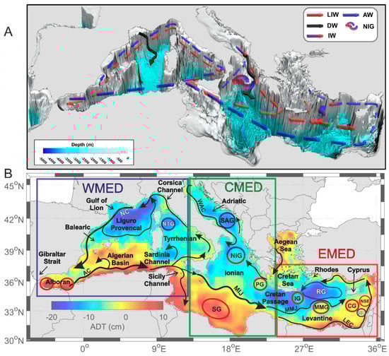
Figure 1.
(A) Schematic representation of the thermohaline circulation in the Mediterranean Sea where the intermediate and deep-water formation sites are highlighted. (B) Geography of the Mediterranean Sea superimposed on the colored mean ADT map for 1993–2019; a schematic representation of the main currents and circulation structures are depicted with black arrows and red (anticyclonic) and blue (cyclonic) circles; geographical extension of the three main sub-basins (WMED, CMED, and EMED). Acronyms: AW, Atlantic Water; LIW, Levantine Intermediate Water; DW, dense water; IW, Intermediate Water; NIG, Northern Ionian Gyre; AC, Algerian Current; NC, Northern Current; NTG, Northern Tyrrhenian Gyre; SG, Sidra Gyre; MIJ, Mid-Ionian-Jet; SAG, Southern Adriatic Gyre; WAC, Western Adriatic Current; PG, Pelops Gyre; MMJ, Mid-Mediterranean Jet; LEC, Libyo-Egyptian Current; IG, Ierapetra Gyre; RG, Rhodes Gyre; MMG, Mersa-Matruh Gyre; CG, Cyprus Gyre; SSE, South Shikmona Eddy; and NSE, North Shikmona Eddy.
Thermohaline properties of the Mediterranean and atmospheric, steric, and mass sea-level variations occur on interannual and decadal scales [13,14,15,16]. Moreover, these variations show prominent long-term trends, which however differ between various sub-basins [11,14,15,17]. These differences are probably due to the local circulation [18,19,20,21], thermohaline changes [22,23,24], and relatively short time-series where it has been calculated from [25,26]. A quick summary of the trend analysis recently conducted in the Mediterranean describes a scenario of increasing freshwater deficit [27], sea surface temperature (SST) and sea level [11,14,15,16], and a basin-scale multi-decadal salinification [11,23,28,29,30]. The SST is considered an important ingredient for the occurrence and intensification of evaporation and heavy precipitation events, and plays an important role on the heat waves in Europe [14,27]. The climatic trends were evidenced not only in the surface layer but also in the thermohaline properties of the intermediate layer [31]. More specifically, it was revealed that LIW temperature and salinity show stronger trend of increase than at intermediate depths in the world ocean [11,31,32,33].
Long-term trends are in turn related to the large-scale atmospheric patterns that influence the weather and climate of the Mediterranean region. The most outstanding climatic index, widely recognized as representative of the atmospheric variability in the northern hemisphere, is the North Atlantic Oscillation (NAO) index, whose positive and negative phases influence the temperature and precipitation patterns of the Mediterranean [34]. However, in addition to the NAO index, there are other indices that are better correlated to heat distribution and trends of the Mediterranean [35]. A recent review on the climatic indices, used as a proxy to monitor the long-term variability of climatic parameters that influence the Mediterranean thermohaline circulation, identifies the Mediterranean Oscillation Index (MOI) as the most suitable option [34].
Nevertheless, Iona et al. [36] show a pronounced multidecadal correlation (significantly larger than that observed with NAO) between the Atlantic Multidecadal Oscillation (AMO) index and the decadal averages of the ocean heat content and ocean salt content.
Interannual and decadal variabilities are related to changes of the thermohaline properties and circulation regimes such as Eastern Mediterranean Transient (EMT), Western Mediterranean Transition (WMT), and Adriatic-Ionian Bimodal Oscillating System (BiOS) [37,38,39,40,41]. The WMT can be defined as a climate shift, which changed the basic structure and properties of the intermediate and deep layers of the western Mediterranean, with an abrupt increase in temperature, salinities, and densities [39,42]; it affects the characteristics of the water exiting the Gibraltar Strait. The EMT is a climatic event that occurred during the 1990s, related to a yet not completely understood chain of atmospheric, oceanic, and hydrological interactions that shift the region of the Eastern Mediterranean deep-water formation from the southern Adriatic to the Cretan Sea [43]. This event influences not only the deep layer but also the entire water column and the circulation structures of the Eastern Mediterranean [19,44]. The BiOS is a feedback mechanism, driven by the difference in salinity between the salty and warmer waters originating in the eastern Mediterranean and the less saline AW entering from the Sicily Channel [39,41,45,46], that is accredited to having led to the quasi-decadal reversal of the Northern Ionian Gyre (NIG) from anticyclonic to cyclonic and vice-versa. Evidence of the importance of this mechanism was obtained by dimensional analysis and laboratory experiments [39,40,41,45,46]. Another possible mechanism proposed for explaining the NIG reversal is wind forcing [47,48,49,50,51]. Grodsky et al. [29] recently proposed a comparison between the temporal variability of the NIG reversals signal and atmospheric forcing (wind stress curl), finding a low anticorrelation and concluding that the NIG circulation modes are probably not atmospherically driven.
The EMT and BiOS occur in different parts of the Mediterranean but nevertheless they extend their impact over the entire basin [52]. The signal associated with these changes, as mentioned above, is mainly advected with LIW flow. It was shown that EMT and WMT are phenomena which occur at time scales longer than decadal, while BiOS is a cyclical quasi-decadal variability of the Ionian and Eastern Mediterranean circulation (NIG reversals) and of its thermohaline properties.
The aim of this work is to study the spatial and temporal (climatic, decadal, and interannual) variability of four oceanographic and air–sea interaction parameters in different Mediterranean sub-areas as well as in the entire basin, in order to estimate what is the relative contribution of different sub-basins to the overall basin-wide variations. For these purposes, in-situ data (Argo float and CTD profiles), satellite (altimetry, SST, and E-P: Evaporation-Precipitation, i.e., freshwater flux), and model (SSS) products are used over the period 1993–2019. Spatio-temporal variability is described, performing the empirical orthogonal function (EOF) analysis on the gridded, monthly, de-seasoned parameters of the whole Mediterranean Sea and of the main sub-basins, which are considered separately. SSS distribution derived from model reanalysis is compared with those derived from in-situ data in the upper layer of the Eastern Mediterranean. The EMT and WMT will be discussed only when they interact or are affected by decadal variability because the available time-series are not long enough to give detailed descriptions of these two phenomena. Special attention will be given to transfer of the signal from the source areas. Possible relationships between the different parameters are delineated and described.
2. Materials and Methods
The datasets used for this study are retrieved from satellite products, in-situ data, and model reanalysis in the period 1993–2019. They are briefly described hereafter:
- The daily (1/8° Mercator projection grid) Absolute Dynamic Topography (ADT) derived from altimeter and distributed by CMEMS (product user manual CMEMS-SL-QUID_008-032-051). The ADT was obtained by the sum of the sea level anomaly and a 20-year synthetic mean estimated by Rio et al. [53] over the 1993–2012 period.
- The daily fields of SST derived from CMEMS (SST_MED_SST_L4_REP_OBSERVATIONS_010_021). This product contains daily mean nighttime SST satellite-based and optimally interpolated (L4) estimates, with a spatial resolution of 0.05° × 0.05° [54,55].
- Monthly surface salinity fields (~1 m depth) derived from the surface MEDSEA products (https://doi.org/10.25423/CMCC/MEDSEA_MULTIYEAR_PHY_006_004_E3R1, downloaded on 20 April 2021) distributed by CMEMS. This product is assessed using a variational data assimilation scheme for temperature and salinity’s vertical profiles; SST and satellite sea level anomaly along track data [56].
- Evaporation and precipitation data downloaded from the hourly ERA5 reanalysis, the fifth generation ECMWF reanalysis for the global climate and weather, that combine model data with observations (doi:10.24381/cds.adbb2d47; [57]). The spatial resolution is 0.25° × 0.25°.
- The Argo float vertical salinity profiles [58] collected in the Mediterranean Sea since 2001 vertically averaged in the surface (0–150 m) and intermediate (200–450 m) layers [59,60].
- Salinity data derived from the Word Ocean Database (WOD; [61]) vertically averaged in the surface (0–150 m) and intermediate (200–450 m) layers.
The gridded datasets obtained from different sources (ADT, SST, E-P) were all averaged over monthly intervals. The SSS data were already downloaded with a monthly temporal resolution, therefore they were not further averaged.
The spatial-temporal variations of these parameters were obtained by performing an empirical orthogonal function s (EOFs) analysis [62] to the gridded monthly datasets. EOF analysis is one of the most widely used and accepted methods to understand the variability in climate data (e.g., Hannachi et al. [63]; Gupta et al. [64]). This method essentially captures the nonlinearity and high-dimensional characteristics for a given dataset, preserving significant patterns and their variability, thereby aiding the users to derive meaningful information for data interpretation and analysis (e.g., Hannachi et al. [63]; Gupta et al. [64]). The EOFs method finds the spatial patterns of variability and their time variations, and gives a measure of the “importance” of each pattern [65]. Before estimating EOFs, all parameters taken at time tj (j = 1, … m) were de-seasoned using a 13-months moving average. EOFs were computed using the classical method [62,65], creating for each dataset (ADT, SST, SSS, E-P) the data matrix F(m,n) where m is the number of spatial grid points and n is the number of months considered. The method removes the temporal mean (see Figure S1 in the Supplementary Materials) from each column, then forms the covariance matrix of F by calculating R = Ft F, solving the eigenvalue problem:
where Λ is a diagonal matrix containing the eigenvalues λi of R (I = 1, … n). The ci column vectors of C are the eigenvectors of R corresponding to the eigenvalues λi. The sizes of Λ and C are n × n. Each eigenvalue λi has a corresponding eigenvector ci; these eigenvectors are the EOFs we are looking for. The first mode of EOFs is the eigenvector associated with the largest eigenvalue; the second mode of EOFs is the second biggest eigenvalue, etc. Each eigenvalue λi gives a measure of the fraction of total variance in R explained by the mode. The eigenvector matrix C has the property that CtC = CCt = I, where I is the identity matrix. This means that the EOFs are uncorrelated over space, or, in other words, the eigenvectors are orthogonal to each other. The pattern obtained when an EOF is plotted as a map represents a standing oscillation. The time evolution of an EOF (principal component time series—PC) shows how this pattern oscillates in time.
RC = CΛ,
In this work, the results of the first two EOFs modes for each parameter (ADT, SST, SSS, and E-P) are analyzed in the whole Mediterranean (MED) and in the three main sub-basins (Figure 1B) separately (geographical limits of the MED sub-basins were adapted from [66]): Western Mediterranean (WMED; 34.5°N–46°N; −6°E–13°E); Central Mediterranean (CMED; 30°N–46°N; 13.5°E–24°E; it includes Adriatic and Ionian seas [67] and the southern Tyrrhenian Sea, as it is affected by the decadal variability induced by the Ionian Sea [20]); and Eastern Mediterranean (EMED; 30°N–37°N; 24°E–36.2°E; the northern Aegean was excluded from the calculation of EOFs in the EMED as it is characterized by very specific local dynamics strongly influenced by exchanges with the Dardanelles).
Linear trends were estimated for the de-seasonalized variables of all the datasets considered. Trends’ accuracy was evaluated using the Mann–Kendall test, a nonparametric method [68,69] commonly employed to detect monotonic trends in a series of environmental, climate, or hydrological data. The purpose of the Mann–Kendall test [68,69,70] is to statistically assess if there is a monotonic upward or downward trend of the variable of interest over time. A monotonic upward (downward) trend means that the variable consistently increases (decreases) through time. The null hypothesis for the Mann–Kendall test is that there is no trend in the series; the alternative hypothesis is that the trend exists. The trends estimated in this work passed the test (the null hypothesis was rejected; 95% confidence level).
A total of two kinds of cross-correlations are computed using the PC of the first and second EOF modes (PCs). The first correlates, for each parameter, the PCs of the MED with the corresponding PCs derived in the three sub-basins. This analysis provides information on how an individual sub-basin behaves in relation to the MED, e.g., whether it affects the MED signal more than another; whether it moves in phase or out-of-phase with the MED. The second cross-correlation was performed between the PCs of different, independent parameters. This analysis combines the fluctuation of different parameters over time, exploring their possible interconnections. The PCs of SSS were not cross-correlated with those of ADT and SST, as the latter variables are assimilated by the model that produces the salinity fields (see Section 2). All the correlations presented in this work are statistically significant (p-values < 0.05 is the probability that the null hypothesis is true, i.e., no correlation is lower than 5%; confidence level 95%), but only those larger than or equal to 0.5 are considered high enough to establish a close link between two sub-basins or between two distinct variables.
A qualitative comparison between the temporal evolution of salinity and those of ADT and SST was performed using in-situ salinity data from the WOD dataset and Argo floats (see Figure S2 for the temporal and spatial distribution of salinity profiles). The sub-basin selected for the comparison is the EMED, as it is the best sampled during the whole period analyzed (1993–2019), both in terms of quantity of data and geographical distribution, and it explained the largest variance of the SSS on the first EOF mode (Table 1).

Table 1.
Explained variance of the EOF1 and EOF2 modes in the MED and in its sub-basins (WMED, CMED, and EMED), time scale involved, and correlation coefficients (p-value < 0–05; 95% confidence level) between the PCs of the MED and those of its sub-basins related to all the parameters considered. Correlation ≥ 0.5 are emphasized in bold in the table and described in the text. Time scales are indicated by Int (interannual), Dec (decadal), and Clim (climatic). The decadal variability linked to the NIG as well as that related to the local structures or to sub-basin dipolar spatial distribution are highlighted in brackets.
Most of the float profiles used in this study were validated using delayed mode quality control (DMQC) technique [71]. The strategy adopted for DMQC is widely described in Wong et al. [59]; Böhme and Send [72]; Owens and Wong [73]; Notarstefano and Poulain [74]; and Cabanes et al. [75]. The accuracy of salinity measurements requested by Argo after the DMQC is 0.01. When DMQC data are unavailable, real-time data are used. Argo float and WOD salinity profiles were vertically averaged in the surface (0–150 m) and intermediate (200–450 m) layers, then they were grouped into three different sub-regions (Figure S2): South Levantine (32–34°N–24–36°E), Crete (34–37°N–24–29°N), and Cyprus (34–37°N–29–36°E). These sub-regions were selected using criteria based both on their specific hydrological characteristics and on data availability (at least one monthly sampling in each of them). Monthly salinity means were obtained in each sub-region and in each layer; hence, a monthly value representing the whole EMED was performed by averaging the values of the three sub-areas for each month.
3. Results and Discussion
This section describes the main results obtained from the EOFs of the four selected parameters: ADT, SST, SSS, and E-P. The spatial pattern of the first and second EOFs modes (hereafter EOF1 and EOF2, respectively) and their amplitude as a function of time (hereafter PC1 and PC2, respectively) are analyzed in detail and discussed in relation to the most recent literature (Section 3.1 and Section 3.2), as well as the possible correlations between independent variables (Section 3.3) and the comparison with in-situ salinity data (Section 3.4). Time series of PC1 and PC2 are shown for each mode and for each parameter in both the MED and its sub-basins (Figure 2, Figure 3, Figure 4, Figure 5, Figure 6, Figure 7, Figure 8 and Figure 9); the spatial patterns (EOF1, EOF2) are always shown for the MED, while they are displayed only in the most interesting cases for the sub-basins, i.e., when the time series and the explained variances describe quite different behaviors with respect to the MED. Table 1 lists the explained variance related to each EOF mode, the time scale explained, the linear trend of the de-seasonalized variables, and the correlations between the PCs of the MED and those of its sub-basins. Time scales described are related to the interannual, decadal, and climatic (larger than decadal) variabilities. Linear trends of the de-seasonalized variables listed in Table 1 are in line with the results of [11,28,40,76,77].
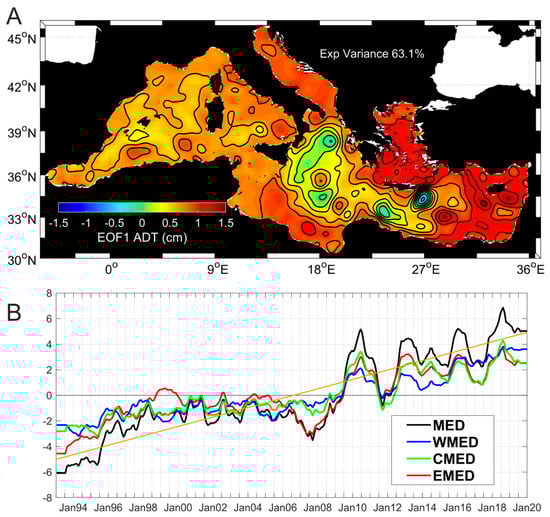
Figure 2.
EOF1 (A) and PC1s (B) of the ADT. The PC1s (B) are estimated for the whole Mediterranean (MED, black line) and for the three main sub-basins separately (West Mediterranean—WMED, blue line; Central Mediterranean—CMED, green line; Eastern Mediterranean—EMED, red line). The long-term linear trend (orange line) is estimated on the PC1 of MED.
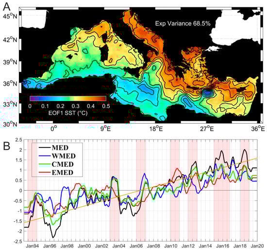
Figure 3.
EOF1 (A) and PC1s (B) of the SST. The PC1s (B) are estimated for the whole Mediterranean (MED, black line) and for the three main sub-basins separately (West Mediterranean—WMED, blue line; Central Mediterranean—CMED, green line; Eastern Mediterranean—EMED, red line). The long-term linear trend (orange line) is estimated on the PC1 of MED. Red shaded areas highlight the period characterized by the occurrence of Mediterranean marine heatwaves, as defined by the recent literature [17,80,81,82,83,84].
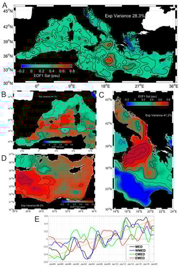
Figure 4.
EOF1 of the SSS for the MED (A), WMED (B), CMED (C), and EMED (D), and relative PC1s (E); the long-term linear trend (orange line) is estimated on the PC1 of MED.
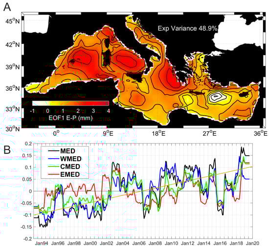
Figure 5.
EOF1 (A) and PC1s (B) of the E-P. The PC1s (B) are estimated for the whole Mediterranean (MED, black line) and for the three main sub-basins separately (West Mediterranean—WMED, blue line; Central Mediterranean—CMED, green line; Eastern Mediterranean—EMED, red line). The long-term linear trend (orange line) is estimated on the PC1 of MED.
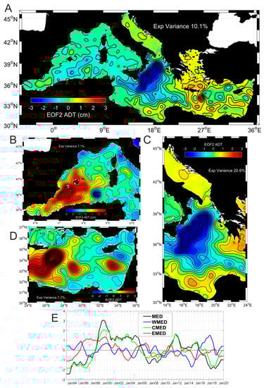
Figure 6.
EOF2 of the ADT for the MED (A), WMED (B), CMED (C), and EMED (D), and relative PC2s (E). The PC2s (B) are estimated for the whole MED (black line) and for the three main sub-basins separately (WMED, blue line; CMED, green line; and EMED, red line).
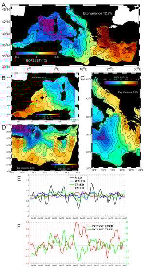
Figure 7.
EOF2 of the SST for the MED (A), WMED (B), CMED (C), and EMED (D), and relative PC2s (E); zoom on the PC2 of the CMED and EMED (F).
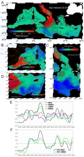
Figure 8.
EOF2 of the SSS for the MED (A), WMED (B), CMED (C), and EMED (D), and relative PC2s (E); comparison between the PC1 of SSS in the CMED and the PC2 of SSS in the MED (F).
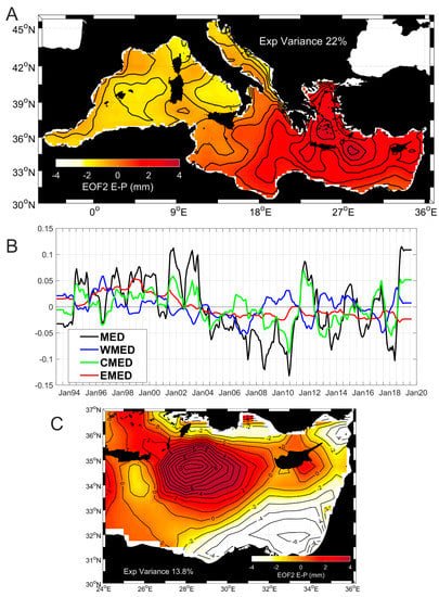
Figure 9.
EOF2 (A) and PC2s (B) of the E-P. EOF2 of the EMED (C).
3.1. First EOF Mode (EOF1)
The EOF1 of the ADT and SST explains 63% and 68% of the data total variance, respectively (Table 1), and captures the interannual and climatic variability of these parameters. The EOF1 and PC1 show a general increase in the sea level and of the SST over the MED (Figure 2 and Figure 3; trends in Table 1 and in Figure 2B and Figure 3B); smaller increases are observed in the northern and central Ionian and in the Cretan Passage. The Ierapetra Gyre (IG) behaves differently from other Mediterranean regions, showing a decrease in sea level (Figure 2A) and a limited increase in temperature in its interior compared to the MED (Figure 3A); this result is in agreement with Mohamed and Skliris [78], who found a significant negative sea level trend in IG and maximum sea level rise in Mersa-Matruh and Cyprus gyres. Considering the three MED sub-basins separately, the EOF1 shows larger explained variances in the EMED (Table 1), both in terms of ADT (72.5%) and of SST (89%). The MED and its sub-basins behave in a consistent way (Figure 2B and Figure 3B), with correlations larger than 0.94 and 0.85 for ADT and SST, respectively (Table 1).
The most prominent and isolated peaks observed in the PC1 of SST (Figure 3B) are associated with occurrences of Mediterranean marine heatwaves (MHWs), qualitatively defined as prolonged periods (five consecutive days or more) of anomalously warm water conditions when compared to the climatological mean (see Hobday et al. [79,80]) and Darmaraki et al. [81] for the definition and classification of MHWs). Based on the analysis of Pisano et al. [17], from 2000 the MED featured the highest SSTs, some of which classified as strong MHWs. The EOF analysis of SST shows whether and to what extent the different MED sub-basins respond to the MHWs events. The signatures of the strong MHWs that occurred in 2003, 2006, and 2017 [17,80,82] are clearly visible in the WMED and CMED, while they are not detected in the EMED (Figure 3B). On the other hand, the event of 2010 [64] involves only the EMED, while that of 2012 [81] involves both CMED and EMED. In 1994, 2015, and 2018, intense summer MHWs affected almost the entire MED [81,83,84], as documented by the increasing temperature in all sub-basins (Figure 3B).
The EOF1 of the SSS in the MED explains 28% of total variance (Table 1; Figure 4A) whereas, considering the sub-basins separately, explained variances exceed 40%, with a maximum in the EMED (66.3%). The PC1s show a general increase in salinity and emphasize the different temporal evolutions among the sub-basins (Figure 4E). The PC1s of SSS in the MED and in the WMED are highly correlated (correlations of ~0.90; Table 1), describing the interannual variability in these regions. In the CMED and the EMED, the most energetic signal is related to the quasi-decadal variability of the NIG circulation (Figure 4C–E). The PC1 in the EMED is out-of-phase with respect to the CMED (correlation coefficient of ~−0.6), in agreement with the results of Gačić et al. [45] and Menna et al. [18]. The largest positive values observed in the northern Ionian and Cretan Passage (Figure 4A,C,D) correspond to surface salinity decreases/increases during the anticyclonic phases of the NIG (1993–1997, 2006–2010, and 2017–2018; negative/positive values of the PC1 in the CMED/EMED; Figure 4E,D) and to salinity increase/decrease during the cyclonic phases (1998–2005 and 2011–2016; positive/negative values of the PC1 in the CMED/EMED; Figure 4E,D), respectively.
The EOF1 and the PC1 of the E-P show a general increase in the freshwater flux in the MED (i.e., evaporation exceeded precipitation; Figure 5A,B), with an explained variance of about 49%. Larger positive values are observed in the Liguro-Provencal Basin, in the Sardinia and Corsica Channels, in the Tyrrhenian Sea, and in the northern Ionian Sea; freshwater flux shows negative values in the region of Rhodes Gyre (Figure 5A). The largest explained variance is observed in the WMED (72.8%), although the EMED shows a slightly lower value (~70%). The PC1 of the E-P in the MED shows a temporal evolution similar to the WMED and CMED (correlations larger than 0.90; Table 1), whereas the EMED is less correlated to the MED (correlation of 0.56).
3.2. Second EOF Mode (EOF2)
The EOF2 and PC2 of ADT in the MED explain 10% of the total variance. Largest variability is observed in the northern Ionian, associated with decadal inversions of the surface circulation (Figure 6A). The NIG shows negative values which, multiplied with the PC2, describes a positive anomaly of sea level in the periods 1993–1997, 2006–2010, and 2016–2018, associated with anticyclonic circulation of the NIG [19,45], and a negative one in the periods 1998–2005 and 2011–2015, associated with cyclonic circulation of the NIG (Figure 6A). The spatial pattern and temporal evolution of the sea level in the MED shows a high correlation (0.94) with the CMED and negligible correlations with the other sub-basins, which are more affected by the local structures’ variability than by the effect of the NIG reversals (Table 1). In the WMED, the more energetic sea level variability is found in the Algerian Basin, while in the EMED it is found in the main sub-basin scale features (IG, Mersa-Matruh Gyre, Cyprus Gyre).
The EOF2 field derived from the SST (Figure 7A) explains 13% of the total variance, showing an out-of-phase behavior between the WMED and the EMED (negative values west of 18°E and positive values on the east), a sort of dipolar configuration centered on the CMED. This dipolar configuration, previously described in Mohamed et al. [15] and Ibrahim et al. [85], also occurs when analyzing the sub-basins separately: the western part of the WMED is out-of-phase with respect to Tyrrhenian Sea (Figure 7B); the western Ionian Sea (west of 18°E) is out-of-phase with respect to the Adriatic Sea and the eastern Ionian Sea (east of 18°E; Figure 7C); the Cretan Sea and the northern Levantine are out-of-phase with respect to the southern Levantine Basin (Figure 7D). The evolution of PC2 in the MED shows a decadal variability unrelated to the NIG reversals (Figure 7E): when the SST increases in the WMED it decreases in the EMED and vice versa. The NIG reversals instead affect the variability of CMED and EMED, which are mainly out-of-phase with each other (Figure 7F): in the CMED (Figure 7C,F) during the NIG anticyclonic/cyclonic mode the SST increases/decreases in the Ionian Sea and decreases/increases in the Adriatic Sea and along the eastern Ionian flank; in the EMED (Figure 7D,F), generally the SST increases/decreases during the NIG anticyclonic/cyclonic mode due to the reduced/enhanced inflow of AW in the Levantine.
The EOF2 and PC2 of SSS in the MED explain 22% of the data total variance and largest variabilities are detected in the northern Ionian and Adriatic seas (Figure 8A); the other regions show negligible values (close to zero), except in the southern Ionian Sea where negative variability describes an out-of-phase behavior compared to the northern Ionian. The PC2 of the MED reproduces the decadal variability associated with inversions of the NIG surface circulation (Figure 8F) and shows a temporal pattern strongly correlated to the PC1 observed in the CMED (the correlation coefficient is 0.82). This result suggests that the quasi-decadal variability of the salinity field induced by the NIG reversals is the dominant signal in the CMED and EMED, occurring in the EOF1, and it is weaker in the whole MED, occurring in the EOF2. Considering the sub-basins separately, the WMED (Figure 8B) and EMED (Figure 8D) show a dipolar configuration, with Alboran and Algerian seas and the Cretan Passage out-of-phase compared to the Liguro-Provençal, and the Tyrrhenian and Levantine, respectively. The EOF2 of the SSS in the CMED (Figure 8C) confirms the opposite behavior of the southern Ionian with respect to the northern Ionian and Adriatic seas, already observed in the EOF2 of the entire MED (Figure 8A).
The EOF2 field derived from E-P (Figure 9; 22% explained variance) shows negative values west of 18°E and positive values on the east, suggesting an opposite behavior between the WMED and the EMED, similarly to the EOF2 of the SST. The evolution of PC2 in the MED shows mainly positive values in the period 1994–2003 and prevalently negative values in the period 2004–2011 (Figure 9B). Positive values of PC2 in the MED indicate the E-P increase in the EMED and its decrease in the WMED; on the contrary, negative values of PC2 are related to the E-P decrease in the EMED and its increase in the WMED. The PC2 of the CMED is highly correlated to the MED (correlation coefficient of 0.84; Table 1), showing an opposite behavior between the Adriatic and the Ionian seas (Figure 9A). In the EMED, the largest E-P variabilities are observed in the region of the RG (Figure 9C). Although the EOF2 of SST and E-P have a similar spatial pattern, the correlations between the PC2 of these variables are not significant (see Table 2). The dipolar behavior observed in the EOF2 of E-P is presumably related to the large-sale atmospheric variability. Criado-Aldeanueva et al. [34] describe a dipolar pattern on decadal scales, which was a correlation between both the NAO and MOI indices and the E-P timeseries in the period 1950–2010. According to these results, E-P shows a positive correlation with the atmospheric forcing (climatic indices) in north-central Mediterranean and a negative correlation in the Levantine.
Table 2.
Correlation coefficients (95% confidence level) between the PC1s and PC2s of the independent variables considered in the Mediterranean Sea and in its sub-basins. Correlation ≥ 0.5 are emphasized in bold in the table and described in the text.
Interpretation of EOF2 modes requires great caution due to the possible artifact resulting from the orthogonality constraint of the EOF technique [86,87]. Nevertheless, these results, showing a dipolar behavior in the second mode of three of the four variables analyzed, suggest that it is peculiar to the variability of the physical field and not an artifact of the statistical method used.
3.3. Correlation between Independent Variables
The correlation coefficients between the PCs of different, independent variables are listed in Table 2. Highest correlations of the PC1s are observed between the sea level (ADT) and the SST both in the MED and in its sub-basins. This result, already obtained by numerous works in the Mediterranean Sea [33,78,88] and at global scales [89], is related to the thermosteric component of sea level variability. The role of the thermosteric component as the major contributor to the linear sea-level trend over the EMED was recently highlighted by Mohamed and Skliris [78].
The correlation between ADT and E-P can be explained in terms of the influence of freshwater fluxes on the mass component of the sea level [13]. This impact is significant in the MED and in the WMED (correlation coefficient of ~0.6), while it is negligible for the EMED. The correlation between SST and E-P shows the effect of freshwater flux on the temperature of the near-surface ocean. This impact, already assessed in the literature at seasonal scales [90], affects the MED at interannual scales (correlation coefficient of ~0.6), while it is less important or negligible in the other sub-basins. The correlation between SSS and E-P represents the influence of the water cycles on the salinity field [11,91]. Larger values, of ~0.5, are estimated in the MED, WMED, and CMED; in the EMED, correlations are negligible. In summary, in the first mode explaining the largest percentage of the total variance, the sea level is mainly thermally driven while the SST is on its turn prevalently determined by air–sea water fluxes (E-P). As far as MED sub-basins are concerned, the sea level is mostly thermally driven in the EMED.
The correlation coefficients between the PC2s of different variables give noticeable results only in three cases (Table 2). In the CMED, the temporal evolution of the ADT, strongly influenced by the effect of the NIG reversals, is in phase with the SST up 2012 (Figure 10A; correlation coefficients of 0.60, Table 2), suggesting the influence of the surface circulation on the temperature distribution in this sub-basin on decadal time scale. In the EMED, the PC2 of ADT, that explains the decadal variability of the main anticyclones (Figure 6E), shows a good correlation (correlation coefficient of ~0.6) with that of E-P, that is related to the decadal variability of Rodes Gyre (Figure 9C). This result suggests a modulation between cyclonic and anticyclonic structures in the EMED with a concurrent reduction of E-P in the Rodes Gyre and of the sea level in the anticyclones from 1995. Looking at the results of the cross-correlations between ADT and E-P obtained from PC1 and PC2 (Table 2), it is clear that the effect of freshwater fluxes is positively correlated with the temporal evolution of the sea level in the MED, WMED, and CMED on interannual scale, and in the EMED on decadal time scales. A similar behavior is observed for the cross-correlations between SSS and E-P obtained from PC1 and PC2; freshwater fluxes affect the salinity distribution in the first mode of the MED, WMED, and CMED, and in the second mode of the MED and EMED.
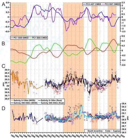
Figure 10.
PC2s of the decadal variability of ADT and SST in the CMED (A); PC1s of the interannual variability of SSS in the CMED and EMED (B); monthly means of the salinity time series in the surface (C) and intermediate (D) layers of the EMED. The monthly salinity values in the three sub-sectors (South Levantine, Crete, and Cyprus) are shown by the black, blue, and red symbols; their average is represented by the solid lines. Anticyclonic periods of the NIG are emphasized in light red.
3.4. Comparison between Model and In-Situ Salinity Data in the Eastern Mediterranean
Salinity fields, obtained from a predictive model and used to perform the EOF analysis, are not independent from the ADT and SST datasets, which are assimilated during the computational process. This would mean that it is not possible to make a quantitative comparison between PCs of SSS and those of ADT and SST. We therefore conducted a qualitative comparison using in-situ salinity data collected by Argo floats in the EMED and those obtained from the model. The EMED was identified as a case study not only because it is the best sampled by Argo floats compared to the other sub-basins, but also because it is the perfect region to appreciate the salinity variations of the Levantine surface water and LIW formed in its interior [92]. These variations affect the variability of the whole MED [4,24,52].
Monthly time series of the WOD and Argo float salinity data in the surface (0–150 m) and intermediate (200–450 m) layers of the EMED (Figure 10C,D, respectively) are compared to the PC1s of SSS in the CMED and EMED (Figure 10B). As described in Section 3.1, the PC1 of SSS in the CMED and EMED are dominated by the variability associated to the NIG circulation reversals, and they are out-of-phase to each other (Figure 10B; correlation coefficient of ~−0.6). In-situ data display a fairly good agreement with the model-derived interannual variability, showing salinity increasements/decreasements in the EMED during NIG anticyclonic/cyclonic modes. This variability is also captured by [31], where an intra-basin variability analysis of the AW and LIW through Argo floats data is provided. The surface and intermediate layers show a similar behavior in term of interannual variability (Figure 10C,D). It is interesting to note that salinity values in the surface layer of the South Levantine sector are lower than the other sectors (red circles in Figure 10C), whereas in the intermediate layer they are in line and occasionally larger than the values collected in the other sectors (red circles in Figure 10D). These salinity values confirm the inflow of the AW in the surface layer of the Southern Levantine, in agreement with the results of Techtmann et al. [93] and Menna et al. [24]. The largest surface layer salinities are observed in the Cyprus sector during the anticyclonic periods (black crosses in Figure 10C) and in the Cretan sector during the cyclonic periods (blue triangles in Figure 10D). The temporary inversion of the NIG from cyclonic to anticyclonic in 2012–2013, caused by the extremely severe winter 2012 [8,46], only affects the surface layer of the EMED (Figure 10C). The effect of decadal variability observed in the intermediate layer can be advected toward the Sicily Channel and then in the WMED [38], becoming a precondition for WMT-like events.
4. Summary and Conclusions
In this article, four oceanographic and air–sea interaction parameters (ADT, SST, SSS, and E-P) were analyzed, both in the MED and in its sub-basins, in order to describe their evolution, connect them to climatic variability, and find their eventual mutual relationships. The role of atmospheric forcing on the MED oceanographic conditions and trends, well demonstrated by several previous studies [16,50,51,78,94], is not directly addressed in this work, which instead focuses on the effect of this forcing rather than on the driving mechanisms. Although the wind conditions and the heat budgets are indirectly considered when describing the evolution of freshwater fluxes (E-P). These variations, which are albeit small in comparison with the total volume of the basin, could produce widespread changes in its physical and biogeochemical properties [95]. In this context, it is important to note that the role of the atmosphere and of the large climate circulation patterns, although very important, mainly influence the Mediterranean multi-decadal variability, which is not fully appreciated in this work due to the too short timeseries, and conversely has a more limited effect on the interannual and quasi-decadal variability. Recent results from Mohamed and Skliris [78] describe an atmospheric contribution to the interannual variability of the sea level of 18%, whereas the steric contribution is 52% in the period 1993–2019.
On the climatic scale, both the MED and its sub-basins behave in a coherent way, showing the seal level, temperature, salinity, and E-P rise over the last 27 years (trends in Table 1 and Figure 2, Figure 3, Figure 4 and Figure 5). Regions with opposite trend are identified in two gyres of the EMED: the IG, where the ADT decreases and the SST increases less than the surrounding regions (Figure 2 and Figure 3); and the Rodes Gyre, where E-P shows a decreasing trend (Figure 5).
The decadal signal associated with the NIG circulation reversals is clearly identified in three of the four parameters considered (ADT, SST, and SSS; see Table 1), in different EOF modes and sub-basins and with different intensities. In the salinity field it appears in the most energetic mode (EOF1) of the CMED and EMED (Figure 4E; Table 1), and it is slightly weaker over the MED, occurring in the second EOF mode (Figure 8E,F; Table 1). For the ADT and SST, the decadal signal associated with the NIG is rather energetic, occurring in the second mode of ADT and in the MED and CMED (Figure 6), and in the second mode of SST in the CMED and EMED (Figure 7F and Figure 10A). The effects of the EMT are not evident from this analysis because they are probably merged with the decadal variability linked to the NIG reversals.
Decadal signals not associated with the NIG circulation reversals appear on the second modes of the considered parameters, strongly related to the variability of local sub-basin structures or to the dipolar behavior between different Mediterranean regions. The ADT in the WMED and EMED sub-basins is more affected by the variability of local structures (Figure 6 and Figure 10A). The surface temperature and E-P show a dipolar behavior between the WMED and the EMED (when SST and E-P increase in the WMED, they decrease in the EMED and vice-versa; Figure 7 and Figure 9).
The influence of wind-stress curl on the decadal variability of MED was not directly addressed in this work, as this comparison was recently performed by [29] using the EOF analysis. These authors found a negligible anti-correlation between the wind forcing and the NIG reversals. The winds and the intensifying NAO atmospheric pressure patterns are considered as co-causes, together with the NIG circulation mode, to the recent thermohaline variability conditions in the EMED.
On an interannual scale, the temporal evolution of the ADT and SST are characterized by high correlation (larger than 0.7; Table 2, i.e., strong influence of the thermosteric component on the sea level) both in the MED and its sub-basins. E-P affects the interannual variability of ADT, SST, and SSS in the MED, WMED, and CMED; it is mainly responsible for the long-term trend of ADT and SSS in the EMED (Table 2). On an interannual scale, the salinity of MED is largely influenced by the WMED (correlation coefficient of 0.87; Table 1), i.e., by the inflow of AW in the basin (Figure 4E, Table 1).
Comparison with in-situ data in the EMED shows that the decadal variability related to the NIG reversals is present in the surface layer associated with the intensity of the AW spreading, which means that both SST and SSS are representative of the entire AW layer; the decadal signal is also evident in the intermediate layer of the EMED, from where it is advected with LIW flow to the other sub-basins and eventually becomes the preconditioning for the WMT-like events.
Supplementary Materials
The following are available online at https://www.mdpi.com/article/10.3390/rs14061322/s1. Figure S1. Mean fields of ADT, SST, SSS and E-P over the period 1993–2019. Figure S2. Temporal distribution of the CTD profiles per month in the EMED (a) derived from WOD (blue) and Argo floats (red) and their positions (b). Green rectangles delimit the three sub-regions (South Levantine, Crete and Cyprus see Section 2) in which profiles were grouped to produce the timeseries in Figure 10C,D.
Author Contributions
Conceptualization, M.M.; writing—original draft preparation, M.M. and M.G.; writing—review and editing, R.M., E.M. and P.-M.P.; methodology, M.M. and M.G.; software, M.M. and R.M.; validation, G.N., R.G. and G.F.; formal analysis, R.M.; investigation, M.M., M.G. and R.M.; resources, G.N. and G.F.; data curation, M.M. and R.M.; supervision, M.G. and P.-M.P.; project administration, E.M. and G.N.; funding acquisition, E.M., P.-M.P. and M.M. All authors have read and agreed to the published version of the manuscript.
Funding
This research was funded by the Italian Ministry of Education, University and Research as part of the Argo-Italy program and by the European Commissions, as part of the Copernicus CMEMS-TAC (82-CMEMS-TAC-INSITU) and Euro-Argo RISE (Grant Agreement number: 824131 —H2020-INFRADEV-2018-2020/H2020-INFRADEV-2018-1 Amendment Reference No AMD-824131-12) programs.
Data Availability Statement
Publicly available datasets were analyzed in this study. These data can be found in: https://nodc.inogs.it/metadata/doidetails?doi=10.6092/7a8499bc-c5ee-472c-b8b5-03523d1e73e9 accessed on 20 April 2021 (the DOI associated to the dataset is: 10.6092/7A8499BC-C5EE-472CB8B5-03523D1E73E9; downloaded on 20 April 2021); https://resources.marine.copernicus.eu/?option=com_csw&view=details&product_id=INSITU_MED_NRT_OBSERVATIONS_013_035 accessed on 20 April 2021, and https://doi.org/10.17882/42182; https://resources.marine.copernicus.eu/products accessed on 20 April 2021; doi:10.24381/cds.adbb2d47; https://www.ncei.noaa.gov/products/world-ocean-database accessed on 20 April 2021.
Acknowledgments
The authors would like to thank all scientists and technicians who deployed floats and made their data available in the Mediterranean Sea. Special thanks to Antonio Bussani, Massimo Pacciaroni, and Antonella Gallo for their technical support in the float preparations, deployments, and data processing.
Conflicts of Interest
The authors declare no conflict of interest.
References
- Jordà, G.; Von Schuckmann, K.; Josey, S.A.; Caniaux, G.; García-Lafuente, J.; Sammartino, S.; Özsoy, E.; Polcher, J.; Notarstefano, G.; Poulain, P.M.; et al. The Mediterranean Sea heat and mass budgets: Estimates, uncertainties and perspectives. Prog. Oceanogr. 2017, 156, 174–208. [Google Scholar] [CrossRef]
- Tsimplis, M.N.; Zervakis, V.; Josey, S.A.; Peneva, E.L.; Struglia, M.V.; Stanev, E.V.; Theocharis, A.; Lionello, P.; Malanotte-Rizzoli, P.; Artale, V.; et al. Changes in the oceanography of the Mediterranean Sea and their link to climate variability, in Mediterranean Climate Variability. In Developments in Earth & Environmental Sciences; Lionello, P., Malanotte-Rizzoli, P., Boscolo, R., Eds.; Elsevier: Amsterdam, The Netherlands, 2006; Volume 4, pp. 227–282. [Google Scholar]
- Menna, M.; Poulain, P.M. Mediterranean intermediate circulation estimated from Argo data in 2003–2010. Ocean Sci. 2010, 6, 331–343. [Google Scholar] [CrossRef] [Green Version]
- Hayes, D.; Poulain, P.M.; Testor, P.; Mortier, L.; Bosse, A.; Du Madron, X. Review of the circulation and characteristics of intermediate water masses of the Mediterranean–implications for cold-water coral habitats. Coral Reefs Mediterranean (CORM). In Coral Reefs of the World; Springer: Berlin, Germany, 2019; Volume 9, pp. 1–26. [Google Scholar] [CrossRef] [Green Version]
- Pinardi, N.; Cessi, P.; Borile, F.; Wolfe, C. The Mediterranean Sea Overturning Circulation. J. Phys. Oceanogr. 2019, 49, 1699–1721. [Google Scholar] [CrossRef]
- Bergamasco, A.; Malanotte-Rizzoli, P. The circulation of the Mediterranean Sea: A historical review of experimental investigations. Adv. Oceanogr. Limnol. 2010, 1, 11–28. [Google Scholar] [CrossRef]
- Houpert, L.; Durrieu de Madron, X.; Testor, P.; Bosse, A.; d’Ortenzio, F.; Bouin, M.N.; Dausse, D.; Le Goff, H.; Kunesch, S.; Labaste, M.; et al. Observations of open-ocean deep convection in the northwestern Mediterranean Sea: Seasonal and interannual variability of mixing and deep water masses for the 2007–2013 Period. J. Geophys. Res. Ocean. 2016, 121, 8139–8171. [Google Scholar] [CrossRef] [Green Version]
- Bensi, M.; Cardin, V.; Rubino, A.; Notarstefano, G.; Poulain, P.M. Effects of winter convection on the deep layer of the Southern Adriatic Sea in 2012. J. Geophys. Res. Ocean. 2013, 118. [Google Scholar] [CrossRef] [Green Version]
- Waldman, R.; Brüggemann, N.; Anthony Boss, A.; Spall, M.; Somot, S.; Florence Sevault, F. Overturning the Mediterranean Thermohaline Circulation. Geophys. Res. Lett. 2018, 45, 8407–8415. [Google Scholar] [CrossRef] [Green Version]
- Kubin, E.; Poulain, P.-M.; Mauri, E.; Menna, M.; Notarstefano, G. Levantine intermediate and Levantine deep water formation: An Argo float study from 2001 to 2017. Water 2019, 11, 1781. [Google Scholar] [CrossRef] [Green Version]
- Skliris, N.; Zika, J.D.; Herold, L.; Josey, S.A.; Marsh, R. Mediterranean sea water budget long-term trend inferred from salinity observations. Clim. Dyn. 2018, 51, 2857–2876. [Google Scholar] [CrossRef] [Green Version]
- Sampatakaki, A.; Zervakis, V.; Mamoutos, I.; Tragou, E.; Gogou, A.; Triantaphyllou, M.; Skliris, N. Investigation of the Inherent Variability of the Mediterranean Sea Under Contrasting Extreme Climatic Conditions. Front. Mar. Sci. 2021, 8, 656737. [Google Scholar] [CrossRef]
- Jordà, G.; Gomis, D. On the interpretation of the steric and mass components of sea level variability: The case of the Mediterranean basin. J. Gephys. Res. 2013, 118, 953–963. [Google Scholar] [CrossRef] [Green Version]
- Pastor, F.; Valiente, J.A.; Palau, J.L. Sea surface temperature in the Mediterranena: Trends and spatial patterns (1982–2016). Pure Appl. Geophys. 2018, 175, 4017–4029. [Google Scholar] [CrossRef] [Green Version]
- Mohamed, B.; Abdallah, M.A.; El-Din, K.A.; Nagy, H.; Shaltout, M. Inter-Annual Variability and Trends of Sea Level and Sea Surface Temperature in the Mediterranean Sea over the Last 25 Years. Pure Appl. Geophys. 2019, 176, 3787–3810. [Google Scholar] [CrossRef]
- Pascual, A.; Marcos, M.; Gomis, D. Comparing the sea level response to pressure and wind forcing of two barotropic models: Validation with tide gauge and altimetry data. J. Geophys. Res. Ocean. 2008, 113, C07011. [Google Scholar] [CrossRef] [Green Version]
- Pisano, A.; Marullo, S.; Artale, V.; Falcini, F.; Yang, C.; Leonelli, F.E.; Santoleri, R.; Buongiorno Nardelli, B. New Evidence of Mediterranean Climate Change and Variability from Sea Surface Temperature Observations. Remote Sens. 2020, 12, 132. [Google Scholar] [CrossRef] [Green Version]
- Menna, M.; Poulain, P.-M.; Zodiatis, G.; Gertman, I. On the surface circulation of the Levantine sub-basin derived from Lagrangian drifters and satellite altimetry data. Deep-Sea Res. Part I 2012, 65, 46–58. [Google Scholar] [CrossRef]
- Menna, M.; Reyes-Suarez, N.C.; Civitarese, G.; Gačić, M.; Poulain, P.-M.; Rubino, A. Decadal variations of circulation in the Central Mediterranean and its interactions with the mesoscale gyres. Deep Sea Res. Part II Top. Stud. Oceanogr. 2019, 164, 14–24. [Google Scholar] [CrossRef]
- Menna, M.; Poulain, P.M.; Ciani, D.; Doglioli, A.; Notarstefano, G.; Gerin, R.; Rio, M.H.; Santoleri, R.; Gauci, A.; Drago, A. New insights of the Sicily Channel and Southern Tyrrhenian Sea variability. Water 2019, 11, 1355. [Google Scholar] [CrossRef] [Green Version]
- Poulain, P.M.; Centurioni, L.; Özgökmen, T.; Tarry, D.; Pascual, A.; Ruiz, S.; Mauri, E.; Menna, M.; Notarstefano, G. On the Structure and Kinematics of an Algerian Eddy in the Southwestern Mediterranean Sea. Remote Sens. 2021, 13, 3039. [Google Scholar] [CrossRef]
- Shabrang, L.; Menna, M.; Pizzi, C.; Lavigne, H.; Civitarese, G.; Gačić, M. Long-term variability of the southern Adriatic circulation in relation to North Atlantic Oscillation. Ocean. Sci. 2016, 12, 233–241. [Google Scholar] [CrossRef] [Green Version]
- Mauri, E.; Sitz, L.; Gerin, R.; Poulain, P.-M.; Hayes, D.; Gildor, H. On the Variability of the Circulation and Water Mass Properties in the Eastern Levantine Sea between September 2016–August 2017. Water 2019, 11, 1741. [Google Scholar] [CrossRef] [Green Version]
- Menna, M.; Gerin, R.; Notarstefano, G.; Mauri, E.; Bussani, A.; Pacciaroni, M.; Poulain, P.M. On the Circulation and Thermohaline Properties of the Eastern Mediterranean Sea. Front. Mar. Sci. 2021, 8, 671469. [Google Scholar] [CrossRef]
- Tsimplis, M.N.; Baker, T.F. Sea level drop in the Mediterranean Sea: An indicator of deep water salinity and temperature changes? Geophys. Res. Lett. 2000, 27, 1731–1734. [Google Scholar] [CrossRef]
- Bonaduce, A.; Pinardi, N.; Oddo, P.; Spada, G.; Larnicol, G. Sea-level variability in the Mediterranean Sea from altimetry and tide gauges. Clym. Dyn. 2016, 47, 2851–2866. [Google Scholar] [CrossRef] [Green Version]
- Romanou, A.; Tselioudis, G.; Zerefos, C.S.; Clayson, C.-A.J.; Curry, A.; Andersson, A. Evaporation-precipitation variability over the Mediterranean and the Black Seas from satellite and reanalysis estimates. J. Clim. 2010, 23, 5268–5287. [Google Scholar] [CrossRef]
- Ozer, T.; Gertman, I.; Kress, N.; Silverman, J.; Herut, B. Interannual thermohaline (1979–2014) and nutrient (2002–2014) dynamics in the Levantine surface and intermediate water masses, SE Mediterranean Sea. Glob. Planet. Chang. 2017, 151, 60–67. [Google Scholar] [CrossRef]
- Grodsky, S.A.; Reul, N.; Bentamy, A.; Vandemark, D.; Guimbard, S. Eastern Mediterranean salinification observed in satellite salinity from SMAP mission. J. Mar. Syst. 2019, 198, 103190. [Google Scholar] [CrossRef]
- Mauri, E.; Menna, M.; Garić, R.; Batistić, M.; Libralato, S.; Notarstefano, G.; Martellucci, R.; Gerin, R.; Pirro, A.; Hure, M.; et al. Recent changes of the salinity distribution and zooplankton community in the South Adriatic Pit. Copernicus Marine Service Ocean State Report, 5. J. Oper. Oceanogr. 2021, 14 (Suppl. S1), 1–185. [Google Scholar] [CrossRef]
- Fedele, G.; Mauri, E.; Notarstefano, G.; Poulain, P.M. Characterization of the Atlantic Water and Levantine Intermediate Water in the Mediterranean Sea using Argo Float Data. Ocean Sci. 2021, 18, 129–142. [Google Scholar] [CrossRef]
- Schroeder, K.; Chiggiato, J.; Josey, S.A.; Borghini, M.; Aracri, S.; Sparnocchia, S. Rapid response to climate change in a marginal sea. Sci. Rep. 2017, 7, 4065. [Google Scholar] [CrossRef] [Green Version]
- Vargas-Yáñez, M.; García-Martínez, M.C.; Moya, F.; Balbín, R.; López-Jurado, J.L.; Serra, M.; Zunino, P.; Pascual, J.; Salat, J. Updating temperature and salinity mean values and trends in the Western Mediterranean: The RADMED Project. Prog. Oceanogr. 2017, 157, 27–46. [Google Scholar] [CrossRef]
- Criado-Aldeanueva, F.; Soto-Navarro, J. Climatic Indices over the Mediterranean Sea: A Review. Appl. Sci. 2020, 10, 5790. [Google Scholar] [CrossRef]
- Mariotti, A.; Dell’Aquila, A. Decadal climate variability in the Mediterranean region: Roles of large-scale forcings and regional processes. Clim. Dyn. 2011, 38, 1129–1145. [Google Scholar] [CrossRef]
- Iona, A.; Theodorou, A.; Sofianos, S.; Watelet, S.; Troupin, C.; Beckers, J.M. Mediterranean sea climatic indices: Monitoring long-term variability and climate changes. Earth Syst. Sci. Data 2018, 10, 1829–1842. [Google Scholar] [CrossRef] [Green Version]
- Roether, W.; Manca, B.B.; Klein, B.; Bregant, D.; Georgopoulos, D.; Beitzel, V.; Kovačević, V.; Luchetta, A. Recent changes in Eastern Mediterranean deep waters. Science 1996, 271, 333–335. [Google Scholar] [CrossRef]
- Schroeder, K.; Josey, S.A.; Herrmann, M.; Grignon, L.; Gasparini, G.P.; Bryden, H.L. Abrupt warming and salting of the WEastern Mediterranean Deep Water after 2005: Atmospheric forcings and lateral advection. J. Geophys. Res. 2010, 115, C08029. [Google Scholar] [CrossRef]
- Gačić, M.; Borzelli, G.E.; Civitarese, G.; Cardin, V.; Yari, S. Can internal processes sustain reversals of the ocean upper circulation? The Ionian Sea example. Geophys. Res. Lett. 2010, 37, L09608. [Google Scholar] [CrossRef]
- Rubino, A.; Gačić, M.; Bensi, M.; Kovačević, V.; Malačič, V.; Menna, M.; Negretti, M.E.; Sommeria, J.; Zanchettin, D.; Barreto, R.V.; et al. Experimental evidence of long-term oceanic circulation reversals without wind influence in the North Ionian Sea. Sci. Rep. 2020, 10, 1905. [Google Scholar] [CrossRef]
- Gačić, M.; Ursella, L.; Kovačević, V.; Menna, M.; Malačič, V.; Bensi, M.; Negretti, M.E.; Cardin, V.; Orlić, M.; Sommeria, J.; et al. Impact of dense-water flow over a sloping bottom on open-sea circulation: Laboratory experiments and an Ionian Sea (Mediterranean) example. Ocean Sci. 2021, 17, 975–996. [Google Scholar] [CrossRef]
- Schroeder, K.; Chiggiato, J.; Bryden, H.L.; Borghini, M.; Ismail, S.B. Abrupt Climate Shift in the Western Mediterranean Sea. Sci. Rep. 2016, 6, 23009. [Google Scholar] [CrossRef] [Green Version]
- Roether, W.; Klein, B.; Manca, B.B.; Theocharis, A.; Kioroglou, S. Transient Eastern Mediterranean deep waters in response to themassive dense-water output of the Aegean Sea in the 1990s. Prog. Oceanogr. 2007, 74, 540–571. [Google Scholar] [CrossRef]
- Civitarese, G.; Gačić, M.; Lipizer, M.; Eusebi Borzelli, G.L. On the impact of the Bimodal Oscillating System (BiOS) on the biogeochemistry and biology of the Adriatic and Ionian Seas (Eastern Mediterranean). Biogeosciences 2010, 7, 3987–3997. [Google Scholar] [CrossRef] [Green Version]
- Gačić, M.; Civitarese, G.; Eusebi Borzelli, G.L.; Kovačević, V.; Poulain, P.M.; Theocharis, A.; Menna, M.; Catucci, A.; Zarokanellos, N. On the relationship between the decadal oscillations of the northern Ionian Sea and the salinity distributions in the eastern Mediterranean. J. Geophys. Res. Oceans 2011, 116, C12. [Google Scholar] [CrossRef]
- Gačić, M.; Civitarese, G.; Kovacevic, V.; Ursella, L.; Bensi, M.; Menna, M.; Cardin, V.; Poulain, P.-M.; Cosoli, S.; Notarstefano, G.; et al. Extreme winter 2012 in the Adriatic: An example of climatic effect on the BiOS rhythm. Ocean Sci. 2014, 10, 513–522. [Google Scholar] [CrossRef] [Green Version]
- Korres, G.; Pinardi, N.; Lascaratos, A. The ocean response to low frequency inter-annual atmospheric variability in the Mediterranean Sea. Part, I. Sensitivity experiments and energy analysis. J. Clim. 2000, 13, 705–731. [Google Scholar] [CrossRef]
- Demirov, E.; Pinardi, N. Simulation of the Mediterranean circulation from 1979 to 1993 model simulations: Part II. Energetics of Variability. J. Mar. Syst. 2002, 33, 23–50. [Google Scholar] [CrossRef]
- Mihanović, H.; Vilibić, I.; Dunić, N.; Šepić, J. Mapping of decadal middle Adriatic oceanographic variability and its relation to the BiOS regime. Geophys. Res. Ocean. 2015, 120, 5615–5630. [Google Scholar] [CrossRef]
- Pinardi, N.; Zavatarelli, M.; Adani, M.; Coppini, G.; Fratianni, C.; Oddo, P.; Simoncelli, S.; Tonani, M.; Lyubartsev, V.; Dobricic, S.; et al. Mediterranean Sea large-scale low-frequency ocean variability and water mass formation rates from 1987 to 2007: A retrospective analysis. Prog. Oceanogr. 2015, 132, 318–332. [Google Scholar] [CrossRef]
- Nagy, H.; Di-Lorenzo, E.; El-Gindy, A. The Impact of Climate Change on Circulation Patterns in the Eastern Mediterranean Sea Upper Layer Using Med-ROMS Model. Prog. Oceanogr. 2019, 175, 226–244. [Google Scholar] [CrossRef]
- Gačić, M.; Schroeder, K.; Civitarese, G.; Cosoli, S.; Vetrano, A.; Eusebi Borzelli, G.L. Salinity in the Sicily Channel corroborates the role of the Adriatic–Ionian Bimodal Oscillating System (BiOS) in shaping the decadal variability of the Mediterranean overturning circulation. Ocean Sci. 2013, 9, 83–90. [Google Scholar] [CrossRef] [Green Version]
- Rio, M.H.; Pascual, A.; Poulain, P.M.; Menna, M.; Barceló, B.; Tintoré, J. Computation of a new mean dynamic topography for the Mediterranean Sea from model outputs, altimeter measurements and oceanographic in situ data. Ocean Sci. 2014, 10, 731–744. [Google Scholar] [CrossRef] [Green Version]
- Pisano, A.; Buongiorno Nardelli, B.; Tronconi, C.; Santoleri, R. The new Mediterranean optimally interpolated pathfinder AVHRR SST Dataset (1982–2012). Remote Sens. Environ. 2016, 176, 107–116. [Google Scholar] [CrossRef]
- Buongiorno Nardelli, B.; Tronconi, C.; Pisano, A.; Santoleri, R. High and Ultra-High resolution processing of satellite Sea Surface Temperature data over Southern European Seas in the framework of MyOcean project. Remote Sens. Environ. 2013, 129, 1–16. [Google Scholar] [CrossRef]
- Escudier, R.; Clementi, E.; Omar, M.; Cipollone, A.; Pistoia, J.; Aydogdu, A.; Drudi, M.; Grandi, A.; Lyubartsev, V.; Lecci, R.; et al. Mediterranean Sea Physical Reanalysis (CMEMS MED-Currents), Version 1; Data Set; Copernicus Monitoring Environment Marine Service (CMEMS): Ramonville-Saint-Agne, France, 2020. [Google Scholar] [CrossRef]
- Hersbach, H.; Bell, B.; Berrisford, P.; Hirahara, S.; Horányi, A.; Muñoz-Sabater, J.; Nicolas, J.; Peubey, C.; Radu, R.; Schepers, D.; et al. The ERA5 global reanalysis. Q. J. R. Meteorol. Soc. 2020, 146, 1999–2049. [Google Scholar] [CrossRef]
- Wong, A.P.S.; Wijffels, S.E.; Riser, S.C.; Pouliquen, S.; Hosoda, S.; Roemmich, D.; Gilson, J.; Johnson, G.C.; Martini, K.; Murphy, D.J.; et al. Argo data 1999–2019: Two million temperature-salinity profiles and subsurface velocity observations from a global array of profiling floats. Front. Mar. Sci. 2020, 7, 700. [Google Scholar] [CrossRef]
- Argo Float Data and Metadata from Global Data Assembly Centre (Argo GDAC); SEANOE: Paris, France, 2020. [CrossRef]
- Wong, A.P.S.; Johnson, G.C.; Owens, W.B. Delayed-mode calibration of autonomous CTD profiling float salinity data by theta-S climatology. J. Atmos. Ocean. Technol. 2003, 20, 308–318. [Google Scholar] [CrossRef] [Green Version]
- Boyer, T.P.; Antonov, J.I.; Baranova, O.K.; Garcia, H.E.; Johnson, D.R.; Mishonov, A.V.; O’Brien, T.D.; Seidov, D.; Smolyar, I.; Zweng, M.M.; et al. World Ocean Database 2013; NOAA Printing Office: Silver Spring, MD, USA, 2013; p. 208. [Google Scholar] [CrossRef]
- Emery, W.J.; Thomson, R.E. Data Analysis Methods in Physical Oceanography; Elsevier Science: Amsterdam, The Netherlands, 2001; pp. 371–567. [Google Scholar] [CrossRef]
- Hannachi, A.; Jolliffe, I.; Stephenson, D. Empirical orthogonal functions and related techniques in atmospheric science: A review. Int. J. Climatol. 2007, 27, 1119–1152. [Google Scholar] [CrossRef]
- Gupta, N.; Bhaskaran, P.K.; Dash, M.K. Dipole behavior in maximum significant wave height over the Southern Indian Ocean. Int. J. Climatol. 2017, 37, 4925–4937. [Google Scholar] [CrossRef]
- Björnsson, H.; Venegas, S.A. Manual for EOF and SVD Analyses of Climate Data; Techical. Report No. 97–1; McGill University: Montréal, QC, Canada, 1997; p. 52. [Google Scholar]
- Pastor, F.; Valiente, J.A.; Khodayar, S. A Warming Mediterranean: 38 Years of Increasing Sea Surface Temperature. Remote Sens. 2020, 12, 2687. [Google Scholar] [CrossRef]
- Verri, G.; Pinardi, N.; Oddo, P.; Ciliberti, S.A.; Coppini, G. River runoff influences on the Central Mediterranean overturning circulation. Clim. Dyn. 2018, 50, 1675–1703. [Google Scholar] [CrossRef] [Green Version]
- Mann, H.B. Nonparametric tests against trend. Econometrica 1945, 13, 245–259. [Google Scholar] [CrossRef]
- Kendall, M.G. Rank Correlation Methods; Oxford University Press: New York, NY, USA, 1975. [Google Scholar]
- Gilbert, R.O. Statistical Methods for Environmental Pollution Monitoring; John Wiley & Sons: Hoboken, NJ, USA, 1997. [Google Scholar]
- Cabanes, C.; Angel-Benavides, I.; Buck, J.; Coatanoan, C.; Dobler, D.; Herbert, G.; Klein, B.; Maze, G.; Notarstefano, G.; Owens, B. DMQC Cookbook for Core Argo Parameters; Ifremer: Plouzané, France, 2021. [Google Scholar] [CrossRef]
- Boehme, L.; Send, U. Objective analyses of hydrographic data for referencing profiling float salinities in highly variable environments. Deep Sea Res. Part II 2005, 52, 651–664. [Google Scholar] [CrossRef]
- Owens, W.B.; Wong, A.P.S. An improved calibration method for the drift of the conductivity sensor on autonomous CTD profiling floats by θ–S climatology. Deep Sea Res. I Oceanogr. Res. Pap. 2009, 56, 450–457. [Google Scholar] [CrossRef]
- Notarstefano, G.; Poulain, P.-M. Delayed Mode Quality Control of Argo Salinity Data in the Mediterranean Sea: A Regional Approach; Technical Report 2013/103 Sez. OCE 40 MAOS; OGS: Sgonico, Italy, 2013; p. 19. [Google Scholar]
- Cabanes, C.; Thierry, V. Lagadec, C. Improvement of bias detection in Argo float conductivity sensors and its application in the North Atlantic. Deep Sea Res. Part I Oceanogr. Res. Pap. 2016, 114, 128–136. [Google Scholar] [CrossRef] [Green Version]
- Von Schuckmann, K.; Traon, P.-Y.L.; Smith, N.; Pascual, A.; Djavidnia, S.; Gattuso, J.-P.; Grégoire, M.; Nolan, G.; Aaboe, S.; Fanjul, E.Á.; et al. Copernicus Marine Service Ocean State Report, Issue 4. J. Oper. Oceanogr. 2020, 13, S1–S172. [Google Scholar] [CrossRef]
- Von Schuckmann, K.; Le Traon, P.Y.; Smith, N.; Pascual, A.; Djavidnia, S.; Gattuso, J.P.; Grégoire, M.; Aaboe, S.; Alari, V.; Alexander, B.E.; et al. Copernicus Marine Service Ocean State Report, Issue 5. J. Oper. Oceanogr. 2021, 14, 1–185. [Google Scholar] [CrossRef]
- Mohamed, B.; Skliris, N. Steric and atmospheric contributions to interannual sea level variability in the eastern Mediterranean Sea over 1993–2019. Oceanologia 2021, 64, 50–62. [Google Scholar] [CrossRef]
- Hobday, A.J.; Alexander, L.V.; Perkins, S.E.; Smale, D.A.; Straub, S.C.; Oliver, E.C.J.; Benthuysen, J.A.; Burrows, M.T.; Donat, M.G.; Feng, M.; et al. A hierarchical approach to defining marine heatwaves. Prog. Oceanogr. 2016, 141, 227–238. [Google Scholar] [CrossRef] [Green Version]
- Hobday, A.J.; Oliver, E.C.J.; Gupta, A.S.; Benthuysen, J.A.; Burrows, M.T.; Donat, M.G.; Holbrook, N.J.; Moore, P.J.; Thomsen, M.S.; Wernberg, T.; et al. Categorizing and naming marine heatwaves. Oceanography 2018, 31, 162–173. [Google Scholar] [CrossRef] [Green Version]
- Darmaraki, S.; Somot, S.; Sevault, F.; Nabat, P.; Cabos Narvaez, W.D.; Cavicchia, L.; Djurdjevic, V.; Li, L.; Sannino, G.; Sein, D.V. Future evolution of Marine Heatwaves in the Mediterranean Sea. Clim. Dyn. 2019, 53, 1371–1392. [Google Scholar] [CrossRef] [Green Version]
- Von Schuckmann, K.; Le Traon, P.Y.; Smith, N.; Pascual, A.; Djavidnia, S.; Gattuso, J.P.; Grégoire, M.; Nolan, G.; Aaboe, S.; Aguiar, E.; et al. Copernicus Marine Service Ocean State Report, Issue 3. J. Oper. Oceanogr. 2019, 12, S1–S123. [Google Scholar] [CrossRef]
- Androulidakis, Y.S.; Krestenitis, Y.N. Surface Temperature Variability and Marine Heat Waves over the Aegean, Ionian, and Cretan Seas from 2008–2021. J. Mar. Sci. Eng. 2022, 10, 42. [Google Scholar] [CrossRef]
- Darmaraki, S.; Somot, S.; Waldman, R.; Sevault, F.; Nabat, P.; Oliver, E. Mediterranean Marine heatwaves: On the comparison of the physical drivers behind the 2003 and 2015 events. In Proceedings of the 22nd EGU General Assembly, Online, 4–8 May 2020; p. 12104. [Google Scholar]
- Ibrahim, O.; Mohamed, B.; Nagy, H. Spatial Variability and Trends of Marine Heat Waves in the Eastern Mediterranean Sea over 39 Years. J. Mar. Sci. Eng. 2021, 9, 643. [Google Scholar] [CrossRef]
- Dommengent, D.; Latif, M. A cautionary note on the interpretation of EOFs. J. Clim. 2002, 15, 216–225. [Google Scholar] [CrossRef] [Green Version]
- Behera, S.K.; Rao, S.A.; Saji, H.N.; Yamagata, T. Comments on “A cautionary note on the interpretation of EOFs”. J. Clim. 2003, 16, 1087–1093. [Google Scholar] [CrossRef] [Green Version]
- Adloff, F.; Somot, S.; Sevault, F.; Jordà, G.; Aznar, R.; Déqué, M.; Herrmann, M.; Marcos, M.; Dubois, C.; Pandoro, E.; et al. Mediterranean Sea response to climate change in an ensamble of twenty first century scenarios. Clim. Dyn. 2015, 45, 2775–2802. [Google Scholar] [CrossRef]
- Aral, M.M.; Guan, J. Global Sea Surface Temperature and Sea Level Rise estimation with optimal historical time lag data. Water 2016, 8, 519. [Google Scholar] [CrossRef] [Green Version]
- Criado-Aldanueva, F.; Soto-Navarro, F.J.; Garcia-Lafuente, J. Seasonal and interannual variability of surface heat and freshwater fluxes in the Mediterranean Sea: Budgets and exchange through the Strait of Gibraltar. Int. J. Climatol. 2012, 32, 286–302. [Google Scholar] [CrossRef]
- Du, Y.; Zhang, Y.; Shi, J. Relationship between sea surface salinity and ocean circulation and climate change. Sci. China 2019, 61, 771–782. [Google Scholar] [CrossRef]
- Malanotte-Rizzoli, P.; Robinson, A. Ocean Processes in Climate Dynamics: Global and Mediterranean Examples; Springer Science & Business Media: Berlin, Germany, 2012; p. 419. [Google Scholar]
- Techtmann, S.M.; Fortney, J.L.; Ayers, K.A.; Joyner, D.C.; Linley, T.D.; Pfiffner, S.M.; Hazen, T.C. The Unique chemistry of Eastern Mediterranean water masses selects for distinct microbial communities by depth. PLoS ONE 2015, 10, e0120605. [Google Scholar] [CrossRef]
- Tsimplis, M.N.; Josey, S.A. Forcing of the Mediterranean Sea by atmospheric oscillations over the North Atlantic. Geophys. Res. Lett. 2001, 28, 803–806. [Google Scholar] [CrossRef] [Green Version]
- Macias, D.; Stips, A.; Garcia-Gorriz, E.; Dosio, A. Hydrological and biogeochemical response of the Mediterranean Sea to freshwater flow changes for the end of the 21st century. PLoS ONE 2018, 13, e0192174. [Google Scholar] [CrossRef] [PubMed] [Green Version]
Publisher’s Note: MDPI stays neutral with regard to jurisdictional claims in published maps and institutional affiliations. |
© 2022 by the authors. Licensee MDPI, Basel, Switzerland. This article is an open access article distributed under the terms and conditions of the Creative Commons Attribution (CC BY) license (https://creativecommons.org/licenses/by/4.0/).