Review

A Review of Synthetic-Aperture Radar Image Formation Algorithms and Implementations: A Computational Perspective

1
INESC-ID, 1000-029 Lisboa, Portugal
2
Instituto Superior Técnico, Universidade de Lisboa, 1049-001 Lisbon, Portugal
3
Instituto Superior de Engenharia de Lisboa, Instituto Politécnico de Lisboa, 1959-007 Lisbon, Portugal
4
Celestia Portugal, 1749-016 Lisbon, Portugal
*
Author to whom correspondence should be addressed.
Remote Sens. 2022, 14(5), 1258; https://doi.org/10.3390/rs14051258
Submission received: 14 January 2022 / Revised: 19 February 2022 / Accepted: 1 March 2022 / Published: 4 March 2022
(This article belongs to the Section Remote Sensing Image Processing)

Abstract

:
Designing synthetic-aperture radar image formation systems can be challenging due to the numerous options of algorithms and devices that can be used. There are many SAR image formation algorithms, such as backprojection, matched-filter, polar format, Range–Doppler and chirp scaling algorithms. Each algorithm presents its own advantages and disadvantages considering efficiency and image quality; thus, we aim to introduce some of the most common SAR image formation algorithms and compare them based on these two aspects. Depending on the requisites of each individual system and implementation, there are many device options to choose from, for instance, FPGAs, GPUs, CPUs, many-core CPUs, and microcontrollers. We present a review of the state of the art of SAR imaging systems implementations. We also compare such implementations in terms of power consumption, execution time, and image quality for the different algorithms used.

1. Introduction

Synthetic-aperture radar (SAR) is a radar-based technology that is capable of generating images of regions or objects, regardless of time of day or weather conditions. SAR has a larger number of applications than other observation technologies, and is used to monitor all sorts of phenomena on the planet’s surface, from crop growth to mine detection, natural disasters, such as volcanoes or hurricanes, to climate change effects, such as the deforestation or melting of glaciers [1].
The most common deployment of SAR is usually in satellites and available through public agencies such as ESA with Copernicus, and NASA with RADARSAT. Recently, tstartups such as Iceye and Capella Space have provided services for high-resolution SAR images on-demand. Unlike optical observation methods, SAR pulses require intensive signal processing before rendering a visible image.
Because of the very computing-intensive SAR signal processing involved, traditionally, SAR signals are collected during a flight and processed offline. Furthermore, with the evolution of silicon and unmanned aerial vehicle (UAV) technologies, it is feasible to equip small aircrafts and drones with SAR sensors and processors, and broadcast the compressed images in real-time. In the selection of the computing platform, it is necessary to account for a tradeoff between three constraints: the algorithm execution time, image quality, and consumed power. Moreover, highly customized hardware accelerators based on field-programmable gate array (FPGA) technology have proposed implementations of systems that achieve better power efficiency than general purpose central processing units (CPUs) [2]. This is of most relevance when considering that these systems are powered by batteries and that the total payload weight is very limited.
This review introduces SAR, different modes of operating, namely stripmap, spotlight and circular, and some of the most common SAR image formation algorithms. A comparison between SAR image formation algorithms is performed, based on execution time and image quality. A state of the art overview and a comparison regarding SAR imaging systems are carried out and compared considering device choices, FPGAs, graphical processing units (GPUs) or CPUs, execution time, image quality and power consumption.

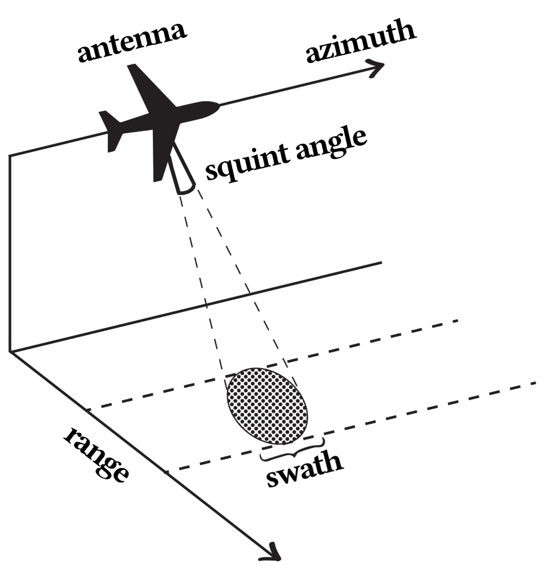
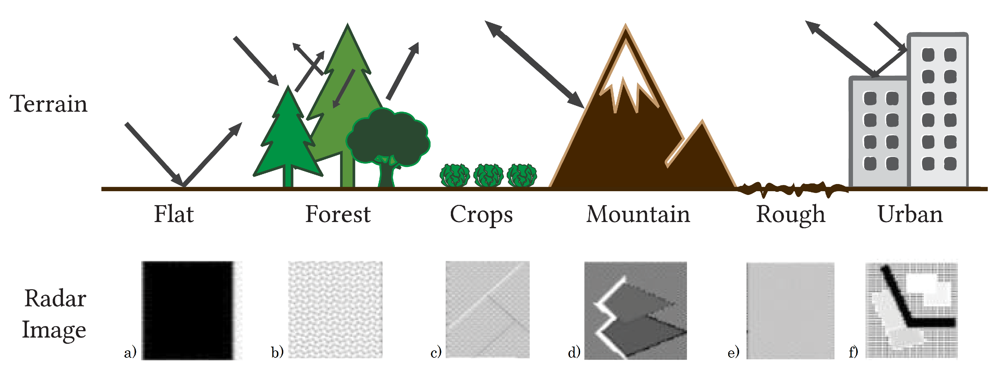
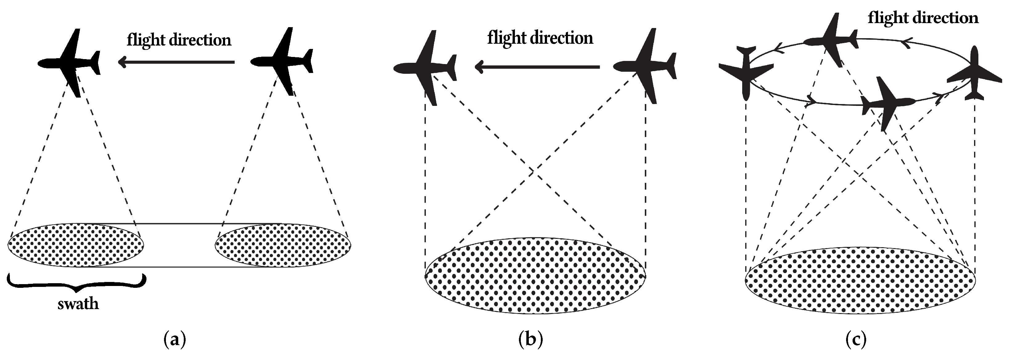
2. Synthetic-Aperture Radar

SAR follows the working principles of radar, emitting electromagnetic waves towards the surface of the Earth, or of objects, and recording the echoes received by the antenna. These echoes are then processed by image generation algorithms, resulting in a synthetic image of a landscape or object. SAR systems use a small antenna which moves along the aircraft or satellite flight path. This creates a larger synthetic aperture when compared to the aperture generated by the same but motionless antenna. Figure 1 illustrates an on-board SAR system in operation. The flight direction is also known as the azimuth direction, and corresponds to the aircraft path. The antenna illuminates a ground region named swath, which is as large as the squint angle. The direction perpendicular to the direction of the flight is named “range direction”.
SAR systems operate at different wavelengths, depending on their intended use. The most common frequency bands and corresponding wavelength are shown in Table 1, [3]. X-band is mostly used for urban, ice, and snow monitoring, due to its weak vegetation penetration. C-band is used for monitoring areas with low-to-moderate vegetation, oceans, and ice. S-band is mostly used for agriculture, ice, and snow monitoring. P- and L-bands are used for vegetation monitoring, subsurface imaging, and biomass estimation [3,4].
Figure 2 illustrates the types of possible reflections due to the elements present in the various scenarios, and the roughness of the materials. A flat surface reflects the signal in a single direction like a mirror, but a rough surface reflects the signal scattered in many directions. Vegetation produces many reflections but is highly attenuated by the multiple reflections between leaves. In the urban landscape, the tops of the buildings produce reflections with the highest intensities, whereas the streets will have the lowest intensities, since most reflections are blocked by the tall buildings.
There are four operating modes for SAR: Stripmap SAR, Spotlight SAR, Circular SAR, and ScanSAR. This review is focused on Stripmap, Spotlight, and Circular SAR [1,5], which are the most used operating modes. These operating modes are illustrated in Figure 3.
Stripmap SAR is a mode of operation where a fixed antenna on a platform, moving in a straight line, continuously emits pulses, illuminating a strip of terrain parallel to the flight path. The main advantage of stripmap SAR is the ability to cover a large area. However, the image quality is inferior when compared to spotlight SAR, described below. A schematic of this operating mode is presented in Figure 3.
Spotlight SAR consists of a platform moving along the straight flight path with a moving antenna. The antenna is constantly moving in order to illuminate the same area continuously. The main advantage of this operating mode is the ability to generate high-resolution images, however, the area that it is able to cover is significantly smaller when compared to Stripmap [5]. Spotlight mode allows the collection of data from different angles, which increases the quality of the image when compared to Stripmap SAR. Spotlight SAR is illustrated in Figure 3b.
Circular SAR consists of a platform performing a circular trajectory, while illuminating the same area at every instance of time. It is similar to Spotlight, however, it follows a circular motion, obtaining data for all 360°, while Spotlight covers 180° in a straight line. The antenna does not move; only the platform it is mounted on. The advantage of this SAR mode is the ability to cover the same region from 360 angles, gathering more information [5]. On the other hand, the resolution of Circular SAR assumes 360° isotropic scattering, and therefore, it is a theoretical resolution. This mode is illustrated in Figure 3c.
ScanSAR consists of an antenna capable of moving in different directions, illuminating different sub-swaths. This mode of operation covers a larger area while sacrificing azimuth resolution [6].
The range ( Δ r ) and azimuth resolution ( Δ a ) of Stripmap, Spotlight, and Circular SAR are displayed in Table 2, where c is the velocity of light, ω 0 is the radar signal half-bandwidth in radians, D y is the diameter of the radar in the azimuth domain, r n is the target radial distance from the center of aperture, λ c is the wavelength at carrier fast-time frequency, λ c = 2 c π ω c , ω c is the central frequency, L is half-size of the aperture, θ n ( 0 ) is the aspect angle of the nth target when radar is at (0, 0), ρ m a x and ρ m i n are the maximum and minimum polar radius in spatial frequency domain for the support of a target at the center of the spotlighted area, k c is the wavenumber at carrier frequency, θ z is the average depression angle of the target area, and ϕ 0 is the polar angle in spatial frequency domain [1]. Table A1 in Appendix A contains the symbols used in this review, their meaning, and units.
A SAR radar emits pulses using a linear FM chirp signal. This signal is defined by Equation (1) [7].
s t ( τ ) = r e c t τ T r × cos 2 π f 0 τ + π K r τ 2
where K r is the chirp rate, f 0 is the carrier frequency, and τ is the range time. The pulse envelope can be approximated using a rectangular function, r e c t τ T r , where T r is the pulse duration. The received signal, or echo, is given by the convolution of the pulse and the ground reflectivity, g r , in the illuminated section,
s r ( τ ) = g r ( τ ) s t ( τ )
Considering the time delay between the emission and reception of the pulse, given by 2 R t / c , where R t is the distance from the antenna to the target and A 0 is the magnitude, the received signal is given by
s r ( τ ) = A 0 r e c t τ 2 R t / c × cos 2 π f 0 ( τ 2 R t / c ) + π K r ( τ 2 R t / c ) 2 + ϕ
where ϕ represents the phase change that may result from the scattering due to the roughness of the reflecting surface.
Since R t changes with azimuth time, it is referred to now as R t ( η ) . Before sampling the signal, it is necessary to remove the radar carrier, cos ( 2 π f 0 τ ) . This is done with a demodulation process, resulting in the following demodulated signal from a single point,
s r ( τ , η ) = A 0 r e c t τ 2 R t ( η ) / c w a ( η η c ) × exp j 4 π f 0 R t ( η ) / c × exp j π K r ( τ 2 R t ( η ) / c ) 2
where w a is the antenna pattern in the azimuth direction, η is the azimuth time and A 0 is a complex constant, A 0 = A 0 exp ( i ϕ ) .

3. Synthetic-Aperture Radar Image Formation Algorithms

There is a wide range of synthetic-aperture radar image formation algorithms. Some recent advances in improving SAR imaging algorithms can be found in [8,9,10]. The following sections describe some of the most used SAR image formation algorithms, such as: Range–Doppler, chirp scaling, omega-K, polar format, matched filter, and backprojection.

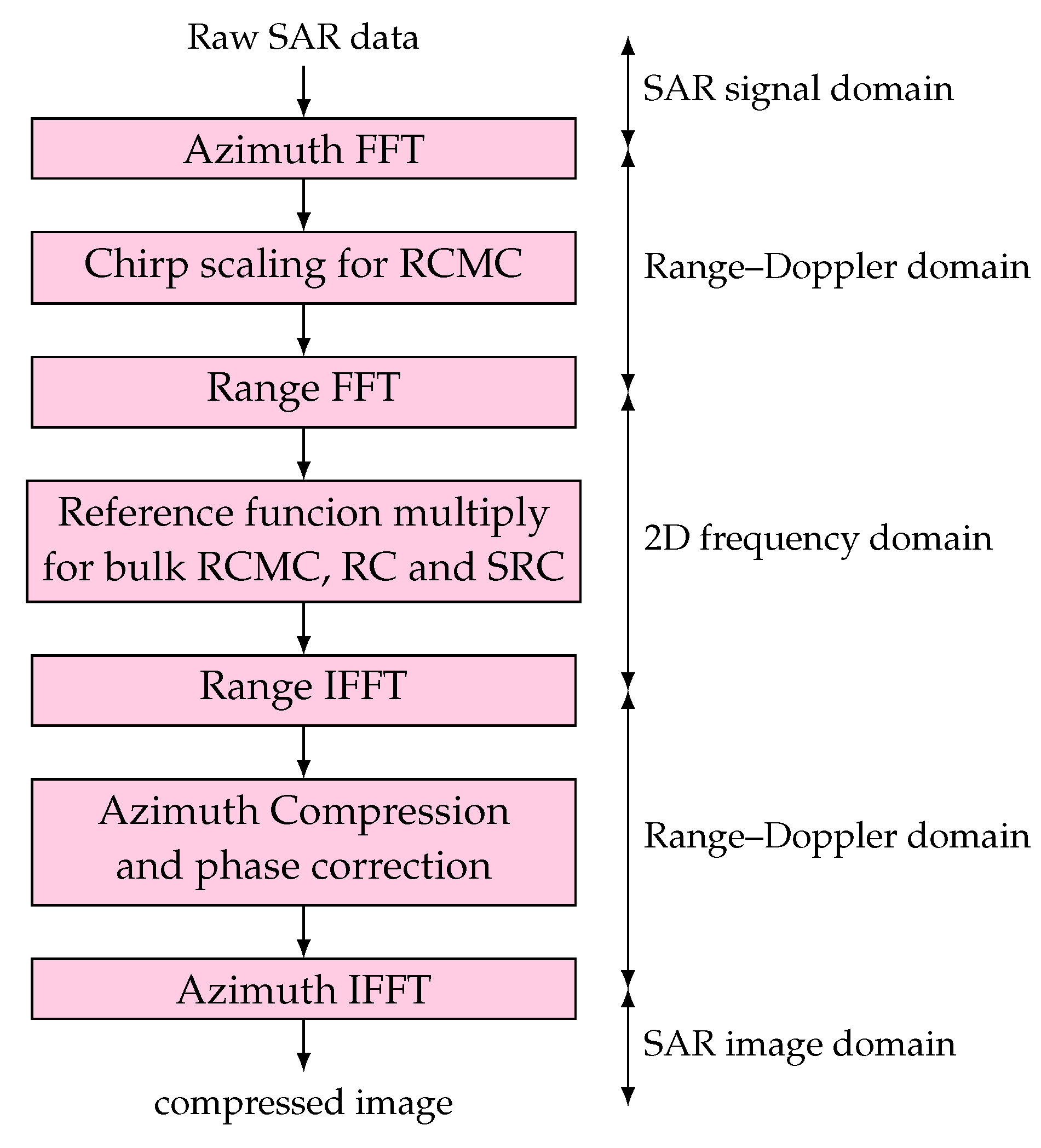
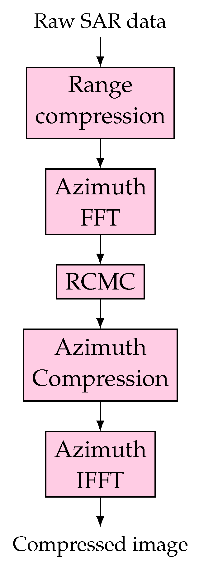
3.1. Range–Doppler Algorithm

The Range–Doppler algorithm was developed in the 1970s, and was used to generate the first SAR digitally processed image. The Range–Doppler algorithm takes advantage of block processing, using frequency domain operations in range and azimuth [7]. The Range–Doppler algorithm is used to generate images with stripmap SAR. A block diagram of the Range–Doppler algorithm is presented in Figure 4. The algorithm consists of the following steps [7]:
1.
A range compression is performed along the range direction, with a fast convolution. This means that a range FFT is performed, a matched filter multiplication and, lastly, a range inverse fast Fourier transform. Using the received demodulation signal given by Equation (4), assuming S 0 ( f τ , η ) is the range FFT of s r and G ( f τ ) is the frequency domain matched filter, the output of this step of the Range–Doppler algorithm is given by
s r c ( τ , η ) = I F F T τ S 0 ( f τ , η ) G ( f τ ) = A 0 p r τ 2 R t ( η ) c w a ( η η c ) × exp j 4 π f 0 R t ( η ) c
where the compressed pulse envelope, p r ( τ ), is the IFFT of the rectangular function.
2.
The data are transformed into the Range–Doppler domain with an azimuth FFT. Since the first exponential in Equation (5) is constant for each target and with f η = K a η , where K a is the azimuth FM rate of point target signal, the output after the azimuth FFT is given by
s 1 ( τ , f η ) = F F T η S r c ( f τ , η ) = A 0 p r τ 2 R r d ( f η ) c W a ( f η f η c ) × exp j 4 π f 0 R t ( η ) c exp j π f η 2 K a
where W a is the envelope of the Doppler spectrum of the antenna beam pattern.
3.
The platform movement causes range variations in the data, a phenomenon called range migration, and hence, a correction is performed to rearrange the data in memory, and straighten the trajectory. This way, it is possible to perform azimuth compression along each parallel azimuth line. This step is called range cell migration correction, and is given by
Δ R ( f η ) = λ 2 R t f η 2 8 V r 2
where λ is the wavelength of carrier frequency f 0 , resulting in the following signal
s 2 ( τ , f η ) = A 0 p r τ 2 R t c W a ( f η f η c ) × exp j 4 π f 0 R t ( η ) c exp j π f η 2 K a
4.
Azimuth compression is performed to compress the energy in the trajectory to a single cell in the azimuth direction. A matched filter is applied to the data after RCMC and, lastly, an IFFT is performed.
The frequency domain matched filter is given by
H a z ( f η ) = exp j π f η 2 K a
After azimuth compression, the resulting signal is given by
s 3 ( τ , f η ) = S 2 ( τ , η ) H a z f η = A 0 p r ( τ 2 R t / c ) W a ( f η f η c ) × exp j 4 π f 0 R t c
5.
Lastly, an azimuth IFFT transforms the data into the time domain, resulting in a compressed complex image. After this step, the compressed image is given by
s a c ( τ , f η ) = I F F T η S 3 ( τ , f η ) = A 0 p r ( τ 2 R t / c ) p a ( η ) × exp j 4 π f 0 R t c exp [ j 2 π f η c η ]
where p a is the amplitude of the azimuth impulse response.
The Range–Doppler algorithm has two main disadvantages. First, there is a need for interpolation during the RCMC step. If high accuracy is needed, the interpolation increases the computational burden. Second, the energy is not entirely concentrated on the range migration curve, as seen above in step 1 of the Range–Doppler algorithm. The spreading of energy introduces degradation into the range focus [11].

3.2. Chirp Scaling Algorithm

The chirp scaling algorithm was developed to remove the interpolator from RCMC in the Range–Doppler algorithm [7,12,13]. The chirp scaling mechanism allows for the implementation of RCMC shift using phase multiplies instead of an interpolator. Initially, the chirp scaling algorithm was developed for Stripmap SAR, however, it has since been adapted to the spotlight mode as well [14]. The following description refers to the stripmap mode only. A block diagram of the chirp scaling algorithm is presented in Figure 5. The chirp scaling algorithm consists of the following steps [7].
1.
The data are transformed into the complex Doppler domain using an azimuth FFT.
2.
Chip scaling is applied, employing a phase multiply, in order to adjust the range migration of the trajectories. Assuming a linear frequency-modulated (FM) pulse, a range invariant radar velocity and a range invariant modified pulse FM rate, K m in the Range–Doppler domain, the scaling function [7] is given by
s s c ( τ , f η ) = exp j π K m D ( f η r e f , V r r e f ) D ( f η , V r r e f ) ( τ ) 2
where K m is the range FM of the point target signal in Range–Doppler domain, f η r e f is the reference azimuth frequency, f η is the azimuth frequency, V r r e f is the effective radar velocity at reference range and D ( ) is the migration factor in the Range–Doppler domain, resulting in the scaled signal in the Range–Doppler domain given by
s 1 ( τ , f η ) = s s c ( τ , f η ) S r d ( τ , f η )
where S r d is given by
s r d ( τ , f η ) = A w r τ 2 R 0 c D ( f η , V r ) W a ( f η f η c ) × exp j 4 π f 0 R 0 D ( f η , V r ) c × exp j π K m τ 2 R 0 c D ( f η , V r ) 2
where A is a complex constant.
3.
The data are transformed into the two-dimensional frequency domain with a range FFT, resulting in the signal given by
s 2 ( f τ , f η ) = A 1 W r ( f r ) W a ( f η f η c ) × exp j 4 π f 0 R 0 D ( f η , V r ) c × exp j π D ( f η , V r ) K m D ( f η r e f , V r ) f τ 2 × exp j 4 π R 0 c D ( f η r e f , V r r e f ) f τ × exp j 4 π c 1 D ( f η , V r r e f ) 1 D ( f η r e f , V r r e f ) R r e f f τ × exp j 4 π K m c 2 D ( f η , V r r e f ) D ( f η r e f , V r r e f ) × R 0 D ( f η , V r ) R r e f D ( f η , V r ) 2
4.
Range compression, secondary range compression (SRC), and bulk RCMC are applied using a phase multiply with a reference function. This step compensates the second and fourth exponentials from Equation (15), resulting in
s 3 ( f τ , f η ) = A 1 W r ( f r ) W a ( f η f η c ) × exp j 4 π f 0 R 0 D ( f η , V r ) c × exp j 4 π R 0 c D ( f η r e f , V r r e f ) f τ × exp j 4 π c 1 D ( f η , V r r e f ) 1 D ( f η r e f , V r r e f ) R r e f f τ × exp j 4 π K m c 2 D ( f η , V r r e f ) D ( f η r e f , V r r e f ) × R 0 D ( f η , V r ) R r e f D ( f η , V r ) 2
5.
Data are converted to the Range–Doppler domain using an IFFT, resulting in a signal in the Range–Doppler domain given by
s 4 ( τ , f η ) = A 2 p r τ 2 R 0 c D ( f η r e f , V r r e f ) W a ( f η , f η c ) × exp j 4 π R 0 f 0 D ( f η , V r ) c × exp j 4 π K m c 2 1 D ( f η , V r r e f ) D ( f η r e f , V r r e f ) × R 0 D ( f η , V r ) R r e f D ( f η , V r ) 2
6.
This step consists of an azimuth compression with a range-varying matched filter, followed by a phase correction and an azimuth IFFT. The matched filter is the complex conjugate of the first exponential of Equation (17). The phase correction is given by the complex conjugate of the second exponential of Equation (17) for linear FM signals. After this step, including azimuth-matched filtering, phase correction and azimuth, the compressed signal at point target is given by
s 5 ( τ , η ) = A 4 p r τ 2 R 0 c D ( f η r e f , V r r e f ) P a ( η η c ) × exp j θ ( τ , η )
where P a ( η ) is the IFFT of the window W a ( f η ) and θ ( τ , η ) is the target phase.

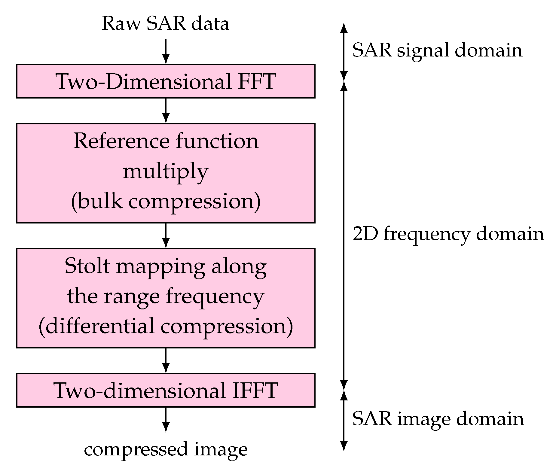
3.3. Omega-K Algorithm

The omega-K algorithm was developed to avoid the range time and azimuth frequency dependency, in the Range–Doppler algorithm, which is not compensated when the azimuth beamwidth is wide, and a range frequency dependency in the chirp scaling algorithm, which is not ideal for high squint angles or wide apertures [7,15,16]. The omega-K algorithm solves these issues with a Stolt operation [17], allowing it to operate over wide azimuth apertures or high squint angles. However, since the omega-K algorithm assumes that the velocity is range invariant, it is not adequate for large-range swaths. Even though the original omega-K algorithm was developed for Stripmap SAR, spotlight alternatives have been implemented [18]. A block diagram of the omega-K algorithm is presented in Figure 6. The main steps of the omega-K algorithm are as follows [7].
1.
Transforming the data into the two-dimensional frequency domain using a 2D FFT, resulted in the baseband uncompressed signal given by
S 2 d f ( f τ , f η ) = A W r ( f τ ) W a ( f η f η c ) × exp j θ 2 d f ( f τ , f η )
2.
Computing the reference function multiply, which is usually computed for the midswath range. Assuming the range pulse is an up chirp with an hyperbolic equation, the phase is given by
θ 2 d f ( f τ , f η ) = 4 π R 0 c ( f 0 + f τ ) 2 c 2 f τ 2 4 V r 2 π f τ 2 K r
By setting the range and effective radar velocity to their midrange or reference values, the phase of the reference function multiplier (RFM) filter is
θ r e f = 4 π R r e f c ( f 0 + f τ ) 2 c 2 f η 2 4 V r r e f 2 + π f τ 2 K r
After applying the filter, the phase remaining is given by
θ R F M 4 π ( R 0 R r e f ) c ( f 0 + f τ ) 2 c 2 f η 2 4 V r 2
The approximation comes from the assumption that V r is range-invariant. This step is called bulk compression.
3.
After the previous step, the data are focused at reference range, and are thus necessary to focus the objects at other ranges. This can be done using the Stolt interpolation, which consists of the mapping of the range frequency axis. This interpolation performs the steps seen in the algorithms presented above, RCMC, SRC, and azimuth compression. The idea of this interpolation is to modify the range frequency axis, replacing the square root in Equation (22) with the shifted and scaled variable, f 0 + f τ , so that
( f 0 p f τ ) 2 c 2 f η 2 4 V r 2 = f 0 + f τ
This results map the original variable, f τ , into a new one, f τ . After the Stolt interpolation, the phase function is given by
θ s t o l t ( f τ , f η ) = 4 π ( R 0 R r e f ) c ( f 0 + f τ )
4.
The last step of this algorithm is a two-dimensional IFFT, transforming the data back into the time domain, and resulting in a compressed complex image.

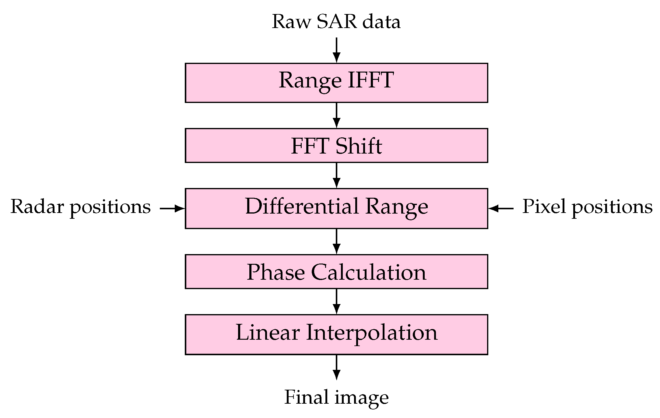
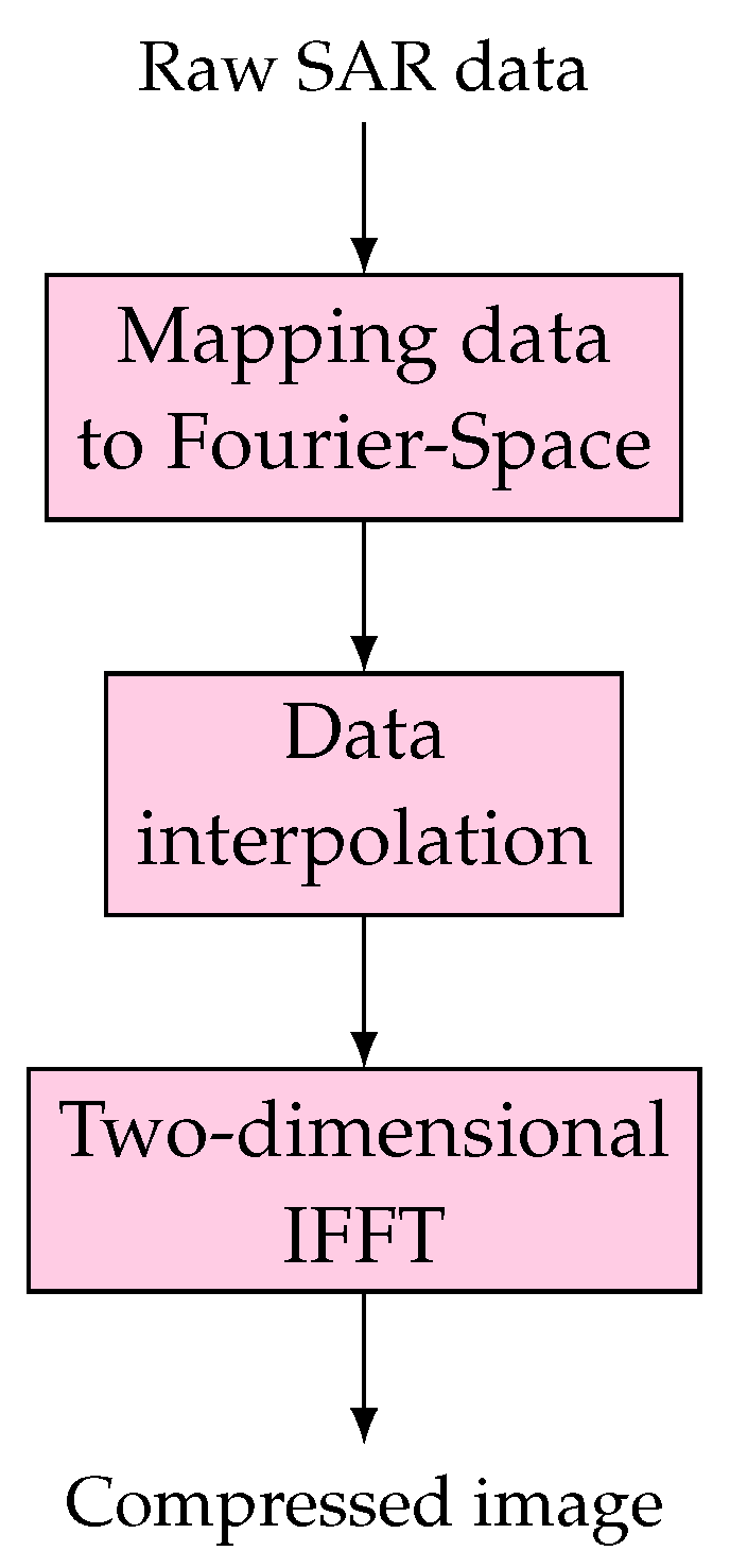
3.4. Polar Format Algorithm

The polar format algorithm is a widely used algorithm for spotlight SAR. Its popularity comes mainly from its computational efficiency, O ( n 2 log 2 n ) . The polar format algorithm is seen as a good alternative if compared to other spotlight formation algorithms [19], such as the backprojection algorithm and matched filter algorithm, described below, with computational complexities of O ( n 3 ) and O ( n 4 ) , respectively. The main difference between the algorithms is the two-dimensional FFT applied in the polar format algorithm, while the backprojection algorithm only applies a FFT in the range domain. The two-dimensional FFT of the polar format algorithm is responsible for the introduction of geometrical warping and the loss of focus in the final image, which increases with distance from the scene center [19,20,21], which can be corrected using several mechanisms [22,23,24].
The key idea of the polar format algorithm is the two-dimensional scattering model which assumes a flat scene, even for three-dimensional SAR systems. The phase history received when using spotlight-operated SAR is a slice of the Fourier transform of the terrain reflectivity, and hence, an inverse FFT can be performed to form an image [22]. This method, however, generates low-resolution images, since the collected data are on a polar grid and the FFT assumes a rectangular one, making it necessary to interpolate the data from the polar to a rectangular grid.
Ideally, a two-dimensional interpolation would be performed, however, it is commonly replaced by an interpolation in the range domain, followed by another in the azimuth domain, for each range line, avoiding the costly two-dimensional interpolation [25].
The steps of the polar format algorithm, illustrated in Figure 7, are as follows.
1.
Map the phase history, or received data, to the correct coordinate of the spatial Fourier transform.
2.
Perform the two-stage interpolation on the K-space data, as described above. This step is going to interpolate the data in a keystone shape to a rectangular grid.
3.
A two-dimensional inverse FFT is performed in the interpolated data, converting the data from the K-space to the Euclidean space, resulting in the final image.

3.5. Matched Filter Algorithm

The matched filter algorithm consists of the application of a matched filter to the received SAR signal, which can be applied to any kind of scatterer. This review considers the implementation described in [23], hence an isotropic point scatterer is assumed. The matched filter of the received signal, at location η in the azimuth, is given by
M F ( η ) = 1 N p K n = 1 N p k = 1 K s r ( τ , η ) exp j 4 π τ Δ R ( η ) c
where N p is the number of pulses and K is the number of frequency samples per pulse. To form an image, Equation (25) is applied for each pixel of the image, resulting in a computational order of O ( N 4 ) .

3.6. Backprojection Algorithm

The backprojection algorithm is based on the projection of the echoes received by the radar, which is performed for each of the image pixels [26]. A block diagram of the backprojection algorithm is given in Figure 8, [27].
The projection of the pulses, or contribution, for every pulse [28], is given by
s ( m , τ n ) = N f f t · F F T s h i f t I F F T ( S ( f k , τ n ) ) × exp j 2 π f 1 ( m 1 ) N f f t Δ f
where N f f t is the FFT length, S ( f k , τ n ) is the phase history, f k is the frequency sample per pulse, τ n is the transmission time of each pulse, f 1 is the minimum frequency for every pulse, m is the range bin and Δ f is the frequency step size. The calculation of each pulse contribution, for every pixel, is calculated from the differential range, that is, the difference between the distance between the radar and the pixel and the range to the scene center, which is used to find the interpolated value of s ( r , τ n ) , s i n t ( r , τ n ) . The differential range is given by
Δ R ( η ) = d a 0 ( τ η ) d a ( τ η ) = ( x a ( η ) x ) 2 + ( y a ( η ) y ) 2 + ( z a ( η ) z ) 2 r 0
where d a 0 ( τ η ) is the distance between the radar and the pixel, d a ( τ η ) is the range to the scene center, also refered to as r 0 , ( x a ( η ) , y a ( η ) , z a ( η ) ) is the position of the radar, or antenna, and ( x , y , z ) is the location of each pixel.
The final value of each pixel at location r is given by the sum of each contribution [28], given by
I ( r ) = n = 1 N p s i n t ( r , τ n )
From Equation (28), the calculation of each pixel is independent, meaning that this algorithm is easily parallelizable. The first two blocks correspond to the IFFT and FFT shift operations present in Equation (26). The differential range block corresponds to the calculation of the distance between the platform and the pixel location.

3.7. Comparison Between Algorithms

Most of the algorithms presented here are frequency-domain algorithms, which also means that they usually have higher computing efficiency. However, the main drawback of such a method is the introduction of side lobes and unfocused regions as the distance to the scene center increases. The backprojection algorithm only performs a range FFT, while the polar format algorithm performs a range and an azimuth FFT, which introduces the side lobes. Of the algorithms presented here, Range–Doppler algorithm, chirp scaling algorithm, omega-K algorithm, and polar format algorithm are frequency-domain algorithms. The matched filter and the backprojection algorithms are both time-domain algorithms and their computational complexity is superior, however, the images do not suffer from the same warping as the previously mentioned algorithms. Table 3 summarizes the main advantages and disadvantages of these algorithms in regard to Level 0 products. For higher-level products, digital elevation models are required when processing SAR data, such as the radiometric terrain correction (RTC) and interferometric SAR (InSAR) products.
The computational load of the Range–Doppler, chirp scaling, and omega-K algorithms evaluated in terms of floating-point operations (FLOPs) published by Cumming et al. [7] identifies the number of necessary operations according to the algorithm section, and then calculates the total number of FLOP for an input with the number of input range samples equal to 4096, number of input range samples per line equal to 4096, interpolation kernel length assumed to be 8, and number of output range samples per line equal to 3072. The results of their analysis are presented in Table 4, where the final number of giga-floating-point operations (GFLOPs) is presented. If desired, the full calculations of these values are detailed in the book [7]. From the table, it is possible to observe that the Range–Doppler algorithm is the one that requires the most GFLOP, while the chirp scaling algorithm requires the smallest number of GFLOP.
Regarding the remaining algorithms, the implementations in which this review was based did not report FLOP, but O-notation. The polar format algorithm is the one with lower computational complexity of O ( n 2 log 2 n ) . As for the time-domain backprojection and matched filter algorithms, the complexity raises to O ( n 3 ) and O ( n 4 ) , respectively.
When it comes down to the algorithm choice, it depends on the system in which the algorithms are going to be executed and, ultimately, the tradeoff between performance, power consumption, and image quality. Computing an image with high resolution will increase the power consumption and computing time, whereas a fast execution with low-power requirements will result in the formation of an image with poor resolution. Image quality is evaluated using the structural similarity (SSIM) metric, described in the next section.

4. Synthetic-Aperture Radar Imaging Implementations

This section describes the state of the art of SAR image formation algorithm implementations, beginning with software implementations, then hardware implementations and GPU/many-core implementations. Following the state of the art, a comparison between several publicly available software implementations is presented, including generated images and execution times. Lastly, a comparison between the hardware accelerators and GPU/many-core implementations is presented.

4.1. Software-Only Implementations

There are several software-only implementations of SAR algorithms widely mentioned in the literature and used as baseline for hardware and other implementations. MatLab is quite user-friendly for the development, analysis, and test of these algorithms. Despite providing highly efficient implementations of data processing, usually it is not used for deployment. The programming language is target dependent, like C programming for software systems, and CUDA-based (Compute Unified Device Architecture) programming for GPU platforms. In the case of custom hardware systems, an accelerator is usually developed that speeds up the processing of the algorithm.
In this review, only freely available implementations of algorithms are presented. Moreover, the authors did not implement any algorithm, as that is not the objective of this work. The backprojection, matched filter, fast-factorized backprojection and polar format algorithm implementations are presented. Hardware implementations were not assessed due to the lack of different platforms and availability.
The backprojection algorithm implementation [28] for circular SAR is the most mentioned in the works described in the following sections. The implementation was designed by LeRoy Gorham and Linda Moore, from the Air Force Research Laboratory (AFRL), and is implemented in MATLAB. They provide not only a complete, ready-to-use MATLAB implementation, but also prepare to take, as input, several datasets made publicly available by the AFRL without needing modifications or pre-processing of data. These datasets are known as the Gotcha Volumetric SAR Dataset [29], Backhoe Data Dome [30], and GMTI Challenge Problem [31].
The SAR image formation toolbox for MATLAB [28] also provides an implementation of the matched filter algorithm. This algorithm implementation is also prepared to receive, as input, the datasets mentioned above.
The fast-factorized backprojection algorithm is an alternative when the backprojection is too expensive, since the computational complexity of this algorithm, O ( n 2 log 2 n ) , is lower when compared to the backprojection algorithm, O ( n 3 ) . A MATLAB implementation of this algorithm was made by Shaun Kelly et al. [32]. This implementation compares the quality of the resulting images depending on the number of iterations performed. The source code of this implementation is publicly available and, similarly to the previous implementations, also takes as input the format of the datasets provided by the AFRL. In the original paper, the Gotcha Volumetric SAR dataset is used to compare the results.
The polar format algorithm implementation [19] in MATLAB provides the source code and is also prepared to receive the data in the format of the datasets of the AFRL.
The backprojection, fast-factorized and matched filter algorithms were implemented for circular SAR. The PERFECT Suite [33] provides a set of applications and kernels for spotlight SAR implemented in C programming language, with CUDA and OpenMP versions. The PERFECT suite provides an implementation of the backprojection algorithm, and two implementations of the polar format algorithm, with different modes of interpolation, range and azimuth. The PERFECT suite provides a dataset in three different sizes of simulated data.
A comparison between the implementations mentioned in this section is performed in the next section, Section 4.2.

4.2. Comparison Between Software-Only Implementations

This section features the comparison between the software implementations discussed in Section 4.1. These implementations are compared in terms of execution time and image quality. To recap, the software implementations compared in this section are the matched filter and backprojection algorithms [28], and fast-factorized backprojection algorithm [32]. These implementations, as mentioned, are written in MATLAB, use the same data format, and are tested using the Gotcha Volumetric SAR dataset [29], the GMTI Challenge Problem [31], and a synthetic dataset that generates point targets, also provided with the backprojection implementation [28].
The PERFECT suite implementations, in C programming language, of the backprojection algorithm and the polar format algorithms, with two interpolations, range and azimuth, are also tested using the synthetic dataset provided.
From the algorithms tested in this review, the matched filter algorithm has the highest computational complexity, O ( n 4 ) , making it impractical for most applications. The images generated by the matched filter algorithm using the GOTCHA Volumetric dataset are presented in Figure 9, the one generated using the GMTI Challenge problem in Figure 10b and the synthetic point target one in Figure 11b. The execution times of the formation of these images are given by Table 5. From this table, it is possible to observe that this algorithm takes between 53 and 517 times longer than any of the others, backprojection algorithm and fast-factorized backprojection. For this reason, it was not possible to generate larger images using this algorithm. Fifty degrees of azimuth takes around 5 hours, and for the GMTI dataset, almost 7 hours. Every image and test presented in this review was executed on a PC desktop with a quad-core Intel Core i7-9700F processor, a NVIDIA GeForce RTX 2060 GPU, 32GB of RAM and 1TB of SSD.
The backprojection algorithm, which has a lower computational complexity of O ( n 3 ) , is a more suitable approach for SAR image formation than the matched filter algorithm. The images using the GOTCHA dataset using this algorithm are presented in Figure 12, the one using the GMTI challenge in Figure 10a and the synthetic point target one in Figure 11a. The execution times are displayed in Table 5, where we can observe the execution times range from 2 s for one degree of azimuth to 12 min for 360° of azimuth.
Lastly, the fast-factorized backprojection algorithm is a more efficient version of the backprojection algorithm, with a complexity of O ( n 2 log 2 n ) . This algorithm was tested with a maximum recursion depth of 4, oversampling ratio of 2, and decimation in phase history. The images from the GOTCHA Volumetric dataset generated using this algorithm are presented in Figure 13, the one using the GMTI challenge in Figure 10c and the synthetic point target one in Figure 11c. The execution times of these tests are available in Table 5, where it is possible to observe that this algorithm takes significantly less time than the backprojection. The largest execution time, the formation of 360° of the azimuth of the GOTCHA dataset, is almost three times quicker than the execution time of the backprojection algorithm.
The images generated using the GMTI dataset with the matched filter, backprojection and fast-factorized backprojection algorithms are presented in Figure 10 and the images generated using the synthetic point target dataset in Figure 11. Since these images are very similar to the naked eye, a metric called SSIM is used to compare them. This metric compares the similarity of two images using three comparison measurments: luminance, contrast and structure. The value of SSIM varies between 0 and 1, with 1 representing an exact copy of the image.
The SSIM values obtained when comparing the images generated using the backprojection algorithm and the matched filter are close to 1, with a difference up to 0.004. This is an expected outcome, since these algorithms generate high-quality images, and the backprojection is able to maintain a quality similar to the matched filter algorithm with a smaller execution time. The fast-factorized algorithm falls behind when it comes to image quality, with a difference in the SSIM values between 0.04 and 0.14. However, it may satisfy the quality requirements for some applications, with its lower execution times. As for the special case of the GMTI image, the SSIM values are so different due to differences in the algorithms, with the backprojection creating dark triangles in the corners while the other two algorithms generate an extremely unfocused region. A fairer comparison is between the matched-filter algorithm generated image, Figure 10b, and the fast-factorized backprojection generated image, Figure 10c. The difference between these two images, represented by the SSIM value, is 0.095399 .
The PERFECT suite provides two different algorithms for SAR image formation: the backprojection algorithm and polar format algorithm, in two versions, with range interpolation, and another with azimuth interpolation. The images generated using the backprojection algorithm are presented in Figure 14, the small input size ( 512 × 512 px), in Figure 14a, the medium input size ( 1024 × 1024 px), in Figure 14b and the large input size ( 2048 × 2048 px), in Figure 14c. The images generated using the polar format algorithm with range interpolation are presented in Figure 15, the small, medium and large images are presented in Figure 15a, Figure 15b and Figure 15c, respectively.
Lastly, the images generated using the polar format algorithm with azimuth interpolation are presented in Figure 16, the small, medium and large images are presented in Figure 16a, Figure 16b and Figure 16c, respectively. In these images it is possible to observe the noise surrounding the bright spots, or point targets, of the synthetic images. The noise is more visible when x = 200 and x = 400 m, approximately, for the small image, when x = 200 , x = 300 and x = 700 m, approximately, for the medium image and x = 600 , x = 1100 , x = 1500 , x = 1900 m, approximately, for the large image.
The execution times of these algorithms vary significantly, as can be observed from the data gathered in Table 6. This table also presents the pixel generation rate in pixels per second (PPS), proportional to the total number of pixels in the image and the time for the algorithm to process them. The execution times vary between 0.06 s and 5.84 s, 0.21 s and 57.91 s and 0.80 s and 9 m 25.04 s for the small, medium and large input datasets, respectively. The polar format algorithm takes at most 1.05 s to generate each image, while the backprojection algorithm takes over nine minutes to generate the larger image. The smaller size is generated by the BP algorithm in 5.84 s, a more reasonable execution time for a 512 × 512 px image.
It should be noted that even though the algorithms are tested with similar datasets of the same three sizes, there are differences in the datasets which do not allow the direct comparison between their quality [33].

4.3. GPU Accelerators for SAR

In this section are described three GPU accelerators for SAR, three high-performance computing (HPC) systems with several nodes, all of which implement the backprojection algorithm, and a solution using a digital-signal processing (DSP) for the Range–Doppler algorithm.
An implementation of the backprojection algorithm for frequency-modulated continuous wave (FMCW) SAR tested on three different devices is presented in [34]. CUDA is used to program the GPU, mainly the NVIDIA CUDA FFT library (cuFFT) and the complex vector operations available in the NVIDIA CUDA Basic Linear Algebra Subroutines (cuBLAS) library. The pixel calculation is calculated using the GPU accelerator, implementing the operations presented in Equation (28). The implementation was tested on a NVIDIA GeForce GT 650 M, on a NVIDIA GeForce GTX 660 Ti, and a NVIDIA Tesla K20c. Compared to a C programming language CPU-based implementation, the NVIDIA GeForce GT 650 M achieves a speedup of 4.9, the NVIDIA GeForce GTX 660 Ti achieves a speedup of 19.5 and the NVIDIA Tesla K20c a speedup of 30.2. Compared to the NVIDIA GeForce GT 650 M implementation, the NVIDIA GeForce GTX 660 Ti achieves a speedup of 4.0 and the NVIDIA Tesla K20c a speedup of 6.2. The implementations were tested using a dataset from a previous experiment of the authors [35].
A real-time GPU implementation of the backprojection algorithm for Stripmap SAR is presented in [36]. The ability to execute the algorithm in real-time comes from the reduction of pulse contributions calculated for each pixel. In its original form, the backprojection algorithm calculates the value of each pixel using every pulse, however, in practice, not all pulses are going to contribute to every pixel. This factor is taken into consideration in this work in order to reduce the computations and reduce the execution time, making real-time a reality for GPU implementations. Data is divided into batches that fit into the GPU memory and processed. Using the texture cache of the GPU, the final execution time is real-time, compared to the original 60 and 70 s, depending on the interpolation. The implementation is tested using the CASIE dataset [37] on a 2008 Mac Pro with a 2-3.2 quad-core Intel Xeon processor, 16 GB of memory and a NVIDIA GTX 285.
An implementation of the backprojection algorithm for GPU is presented in [38]. It should be noted that this implementation, unlike the others presented in this review, performs a considerable part of the computation, i.e., the pre-processing, in MATLAB or Python and uses this data as input for the final implementation. This pre-processing includes the application of a sliding window to the data, filtration for frequency deweighting and inverse FFT. Similarly to other works, this implementation takes advantage of the texture cache of the GPU for interpolated values. The input data is divided into batches, processing sub-images simultaneously. The final result is tested using the Volumetric dataset, or GOTCHA, Ref. [29] and the GMTI dataset [31], both provided by the AFRL. For the GOTCHA dataset, a single-threaded C application executed on a quad-core 2.66 GHz Intel Xeon processor is compared to the CUDA implementation executed on a NVIDIA Quadro FX 5600. When it comes to the GMTI dataset, the same C application is compared to the CUDA implementation on a NVIDIA Tesla C1060. The speedup obtained ranges from 40 to 60, depending on the block size used, when compared to the original version.
Due to the intensive signal processing required to generate SAR images, real-time implementations are a challenge. HPC systems have a large computing capabilities, thus being used for real-time implementations of SAR algorithms. With a cluster of four nodes, Ref. [39] presents an implementation for Stripmap SAR. The received signals are divided into sections and sent to different nodes. The resulting image sections overlap among themselves and are merged after the algorithm execution. Using four nodes, where each node is composed of two Intel Xeon E5-2690v3 and 4 NVIDIA Tesla M60 GPU, the image is generated in 1.0 s, after receiving the raw data during 17.7 s. The final configuration shows a speedup of 11.5 when compared to a single GPU.
Another real-time implementation of the backprojection algorithm is presented in [40]. In this implementation, several approximate strength reduction optimizations, such as quadratic polynomial approximations, Taylor series as square root calculation method and trigonometric function strength reduction, are used to reduce the computational load of the algorithm. The computation is partitioned between Intel Xeon and Intel Xeon Phi processors and MPI and OpenMP is used to program the system. A single node is able to generate a 3000 × 3000 px image in real-time while 16 nodes are able to generate a 13,000 × 13,000 px image in real-time.
Using the implementation of the backprojection algorithm presented in Section 4.1 [28], Ref. [41] presents an accelerator for the backprojection algorithm. Calculating 1 degree of azimuth data using C/MPI code takes 4.7 s for a 512 × 512 px image, whereas only takes 0.15 seconds using the GPU, resulting in a speedup of 31×. Speedup increases with the image size, as for 2048 × 2024 px images the speedup increases to 55× and for 4096 × 4096 px images the speedup achieves 58×. The implementation was tested on 4 nodes of the Ohio Supercomputer Center’s BALE Visualization GPU cluster, each with two 2.6 GHz AMD Opteron processors and a NVIDIA Quadro 5600 GPU.
Lastly, a real-time implementation of the Range–Doppler algorithm using a DSP is presented in [42]. The device used is a TMX320C6678 DSP from Texas Instruments and provides 128 GLOPs in single precision. In this implementation, the raw data is stored in the DDR3 memory and transmitted using EDMA3. The input data is divided into 8 portions and each core processes one portion. This implementation is able to generate a 4096 × 4096 px pixel image in only 0.25 s, in other words, in real-time, with a power consumption of 10 watts.
The works described in this section are summarized in Table 7. This table includes the algorithm, execution times, whether it runs in real-time or not, devices used and additional notes, such as obtained speedups, image quality metrics and power consumption.
Final remarks on the implementations mentioned in this section and Section 4.4 are made in Section 4.5.

4.4. Hardware Accelerators

Software implementations tend to take longer to execute and have a higher power consumption when compared to hardware implementations. Many hardware implementations of SAR image formation algorithms exist due to these benefits.
An implementation of the backprojection algorithm capable of generating real-time images with 60,000 pixels with resolution of 2 × 2 meters is presented in [43]. This implementation uses 64 Tinuso cores [44], a soft processor, with a 2D mesh interconnect. The device used to implement this design was a Xilinx Virtex-7 7VX550T FPGA, with 60% of 550 thousand logic elements used and a clock speed of 300 MHz. A single-precision floating point unit (FPU) is used to implement basic arithmetic operations and square root, while sinc, sine and Hamming window functions are implemented using look-up tables. With the real-time requisites, the final system consisted of 64 cores and 4 memory controllers with a power consumption of 10 watts. It is important to note that this implementation is merely simulated, not being tested on the device itself.
Cholewa et al. present the implementation of the backprojection algorithm using the Unified Emulation Framework (UEMU) [45]. This framework allows the development of hardware for different devices, such as software-defined radio (SDR) platforms, FPGA and application-specific integrated circuits (ASIC). A backprojection module was developed to generate one line of the final image at a time, looping over all pulses for each line. To calculate the square root and trigonometric functions, sine and cosine, a coordinate rotation digital computer (CORDIC) is used. The results obtained show that the implementation scales almost linearly with the parallelization factor. Using a Virtex-6 FPGA ML605 Evaluation Kit, running at 100 MHz, the execution has a speedup of 68 with a parallelization factor of 8 when compared to a software implementation in MATLAB [28] on an Intel i5 3.2 GHz with 4 cores. This implementation occupies 78% of LUTs, 62% of BRAMs and 40% of DSPs. The execution times were 0.03 s, 0.18 s, 1.44 s and 10.94s for square images with N equal to 256, 512, 1024 and 2048, respectively.
Backprojection units were developed in another implementation of the backprojection algorithm for FPGA [26]. These units are independent and can be used as many as they fit into the target device. Each unit is responsible for receiving raw data and generating a pixel contribution, which is then added to the current pixel value. In this implementation, an Arria-V SoC from Altera is used, which also integrates an ARM Cortex-A9 dual-core processor. In this device, 20 backprojection cores were used, and the accelerators on the FPGA ran at a clock frequency of 133 MHz. The final image, using the GOTCHA dataset [31], is calculated in 120.34 milliseconds, with a total power consumption of 26.55 watts.
A design for ASIC in 65nm complementary metal–oxide–semiconductor (CMOS) is presented in [27]. The device has a clock frequency of 1.2 GHz and implements in hardware the MATLAB version of the algorithm [28]. The authors of the work realize it is possible to decrease the precision of the algorithm while still obtaining high quality images. The algorithm is divided into blocks, each block with a customized floating-point data representation. Ultimately, the objective of the authors is to decrease the mantissa as much as possible, while maintaining the SSIM metric above 0.99. More details on this metric are provided in Section 4.2. This work does not mention execution times, only the ability to save 75.5% of area using mantissa widths between 6 and 27 bits.
An implementation of the Range–Doppler algorithm using four Xilinx Virtex-6-550T devices with 16 processing elements split among the 4 devices is presented in [46]. The communication between these elements uses a message passing scheme and a 2D mesh interconnect floating-point calculations are supported using the Xilinx FPU, which allows the calculation of basic arithmetic operations and square root and a look-up table is used to calculate the Hamming window and sine functions. The final implementation is able to generate 2048 × 4096 px images in 12.03 s, running at 130 MHz, with 67% of logic elements occupied and a power consumption of 85 watts, compared to 189.34 seconds when a Intel Core i7-930 processor at 2.8 GHz is used, reaching a speedup of 15.74. The authors calculated the Peak Side Lobe Ratio (PSLR)f and Mean Squared Error (MSE), which have almost identical values, however, do not specify values.
An implementation of the polar format algorithm using FPGA is presented in [47]. This implementation uses a floating-point data representation, except when the CORDIC algorithm is used, when the data are converted to fixed-point. The whole system was tested on a Xilinx Kintex-7 XC7K325T-2FFG900C evaluation board and is able to generate a 4096 × 4096 px image in approximately 1 second. The FPGA runs at a clock speed of 200 MHz and the implementation occupies 68% of LUTs, 48% of registers, 42% of BRAMs and 96% of DSP. When it comes to quality metrics, they obtained a range PSLR of −28 dB and range resolution of 2.65 m, an azimuth PSLR of −40 dB and an azimuth resolution of 1.03 m.
Ref. [48] presentes a system composed of nodes with dual 2.2 GHz Intel Xeon processors running Linux and an Annapolis Microsystems WildStar II FPGA accelerator board with two Xilinx Virtex-II FPGA. The software is programmed using MPI, and is used to set up the FPGA and to read the radar data. The radar data is also converted from floating-point to fixed-point and then the data is organized into chunks and sent to the FPGA. The backprojection algorithm is implemented in hardware. The input is simulated data [1]. The application uses 36-bit complex integers (18-bit real and 18-bit imaginary) and is able to achieve speedups between 167.4 and 217.6, depending on the dataset, for the backprojection algorithm. The complete app, which includes image formation, achieves speedup values between 49.8 and 108.4×. The FPGA are able to run at 133 MHz of clock frequency.
Lastly, an implementation of the Range–Doppler algorithm is presented in [49]. This implementation was tested using a DE2-115 Terasic Development Kit, based on a Cyclone E IV (60 nm) FPGA running at 50 MHz of clock frequency, and uses a NIOS II soft processor. The FFT and IFFT functions are implemented in hardware, while the rest is performed in software. The total execution of this implementation takes 20.31 s for a 2048 × 2048 px image and occupies 57% of LUTs, 31% of registers, 21% of BRAMs and 56% of DSP.
The works described in this section are summarized in Table 8 and Table 9. Table 8 includes the algorithm, execution times, whether the work is real-time or not, image dimensions and quality metrics. Table 9 includes the device, clock frequency, hardware resources, power consumption and additional comments. Notes marked with an asterisk are displayed in the last column of Table 9, named Notes. Few works (three of eight) do not report power consumption, which can be an important requisite when designing systems. [49] is capable of computing a 2048 × 2048 image within a second. However, it is based on the Range–Doppler algorithm which generates not so good images. Similar result was reported by [47] using the polar format algorithm. On the other hand, backprojection generates images with higher quality but for the same image size [45] required more than 35× of the execution time.

4.5. Comparison Between GPU and Hardware Implementations

Following the comparison presented in the last section, a final comparison of the works detailed in this review in Section 4.4 and Section 4.3 is warranted.
There are several hardware implementations already published. As can be seen in Table 8 and Table 9, which present the details of the papers described for easier comparison, most works lack in quality metrics and power consumption information. Only three of the five Backprojection algorithm implementations presented in this review are executed in real-time and are using at the time of publication high-end devices such as the Altera Arria-V SoC [26] and Xilinx Virtex-7 [43] or many-core systems, namely a dual-core Intel Xeon processor with an Anapolis Microsystems WildStar II FPGA board with two Virtex-II FPGA [48]. The first work was only simulated and the reports are given by the simulation tool, Xilinx Vivado. The many-core implementation with FPGA [48], even though the authors do not report the exact numbers in their paper, has a higher power consumption than the rest of the implementations. The implementation achieves speedup values between 49.8 and 108.4 times, depending on the dataset. The polar format algorithm implementation [47] generates images in real-time, using a Xilinx Kintex-7 FPGA. The polar format algorithm, more efficient than the others, is a suitable alternative for real-time applications when the warping and side lobes do not represent a main concern.
Lastly, GPU and other many-core systems are a great option when power consumption is not a concern due to their high performance. Table 7 presents the details of the works mentioned in Section 4.3. As can be observed, power consumption not reported in any of the works mentioned in this review except for the DSP implementation [42]. This work implements the Range–Doppler algorithm, known for its simplicity and efficiency. Five out of the nine implementations of the Backprojection algorithm presented in this review are real-time, even for images with dimensions as large as 13 K × 13 K px.

4.6. Precision Analysis

One of the main concerns when implementing algorithms using accelerators is the tradeoff between performance and precision. This is specially true for hardware accelerators, where operations are commonly implemented using fixed-point notation due to the overhead introduced by the implementation of floating-point units. GPU implementations tend to use single precision values instead of double precision, either because the devices do not support it or because of the overhead introduced. In an attempt to show the influence of precision in SAR algorithms, this section presents the results of testing the PERFECT [33] implementation of the Backprojection algorithm with variables in single-precision only and the original implementation of the algorithm where most of the variables are in double-precision, including intermediary calculations, except the phase history and final image.
The images generated are compared with the golden reference images, provided in the PERFECT suite. The results of these tests are presented in Table 10. Figure 17 presents the images generated in this test, Figure 17a is the golden reference of the small dataset, Figure 17b is the image generated using the original implementation, with variables in single and double-precision, and, lastly, Figure 17c is the image generated using single-precision only. There is no difference to the naked eye between Figure 17a, the golden reference, and Figure 17b. There is, however, difference between these two and the single-precision image, Figure 17c. It is possible to see the noise when x = 200 and x = 400 .
Regarding the execution time, it heavily depends on the system where the computation happens. For example on a modern Intel Core i7-9700F CPU, running at 3.0 GHz, the difference between single and double precision is less than one second out of a total of 5.8 s for the double precision case. This variation in the execution which may not be significant for most use cases, but the quality varied from 15 dB, for the single-precision, to 138 dB, for the double-precision. To make the difference more apparent, this test was performed on a Zynq UltraScale+ MPSoC ZCU104 Evaluation Kit, with a ZU7EV device with a quad-core ARM Cortex-A53 and a dual-core ARM Cortex-R5 processors. The execution time of the application running on a single core of the ARM Cortex-A53 is 270.80 s for the original version and 259.75 s for the single-precision version. There is a significant difference in the SNR of the generated images, less 90% than the original version, and a difference of 10 in the SSIM. To sum up, the execution time will depend more on the performance of CPU where the computation happen, and less on the wordlength. Custom reconfigurable architectures are able to perform more efficiently than general purpose CPUs. Yet, any savings in the execution time, by considering smaller wordlengths, will lead to the loss of quality in the resulting image.

5. Conclusions

This review presented an introduction to the topic of SAR, including SAR functioning, different types of SAR, namely stripmap, spotlight and circular SAR, some of the most used SAR image formation algorithms and a comparison between them. Furthermore, a review of the state of art was presented, describing accelerators for different SAR algorithms implemented in hardware, GPU, HW/SW solutions and software implementations of SAR algorithms. These software implementations, publicly available, were compared and their generated images, execution times, and image quality metrics were assessed.
Designing SAR imaging systems can be challenging, especially when deciding the algorithm to implement and the target device. This review introduced SAR image formation algorithms, their advantages, and described the trade-off between image quality and efficiency. As a conclusion, frequency-domain algorithms are more efficient, however, the image quality is inferior when compared to other time-domain algorithms.
Real-time implementations of SAR image formation algorithms are available in the literature, and most take advantage of the efficiency of frequency-domain algorithms. Real-time systems with higher performance and increased power consumption are available, however, do not satisfy the requisites for on-board systems which are battery-powered.
The choice regarding SAR image formation algorithms depends on the requisites of the application or system. Execution times, power efficiency and image quality are factors that need to be taken into consideration when deciding. On-board systems cannot provide the necessary energy for GPU or other many-core systems, making hardware devices a good alternative. However, when performance and speed is the main concern and power efficiency is not an issue, GPU devices are great alternatives. The Backprojection algorithm provides high-quality images, however, with a larger overhead, while the frequency-domain algorithms mentioned in this review, Range–Doppler, chirp scaling, omega-K, and polar format algorithms have a lower computational complexity.

Author Contributions

Conceptualization, H.C. and R.P.D.; methodology, H.C. and R.P.D.; software, H.C.; validation, H.C. and R.P.D.; formal analysis, H.C.; investigation, H.C. and R.P.D.; resources, R.P.D. and H.N.; data curation, H.C.; writing—original draft preparation, H.C.; writing—review and editing, M.V., J.M., H.N. and R.P.D.; visualization, H.C.; supervision, J.M., H.N. and R.P.D.; project administration, R.P.D. and H.N.; funding acquisition, R.P.D. and H.N. All authors have read and agreed to the published version of the manuscript.

Funding

This work was supported by national funds through Fundação para a Ciência e a Tecnologia (FCT) with references UIDB/50021/2020 and PTDC/EEI-HAC/31819/2017 (SARRROCA). Helena Cruz would like to acknowledge Fundação para a Ciência e a Tecnologia for the support through grant SFRH/BD/144133/2019.

Institutional Review Board Statement

Not applicable.

Informed Consent Statement

Not applicable.

Data Availability Statement

This review used and analysed the following publicly available datasets: Gotcha Volumetric SAR Dataset (https://www.sdms.afrl.af.mil/index.php?collection=gotcha, accessed on 12 June 2019) [29], GMTI Challenge Problem (https://www.sdms.afrl.af.mil/index.php?collection=gmti, accessed on 25 November 2020) [31] and PERFECT Suite (https://hpc.pnl.gov/PERFECT/, accessed on 14 April 2020) [33].

Conflicts of Interest

The authors declare no conflict of interest.

Abbreviations

The following abbreviations are used in this manuscript:
AFRLAir Force Research Laboratory
ASICApplication-Specific Integrated Circuit
BRAMBlock Random-Access Memory
CMOSComplementary Metal–Oxide–Semiconductor
CORDICCOordinate Rotation DIgital Computer
CPUCentral Processing Unit
CUDACompute Unified Device Architecture
DSPDigital-Signal Processing
EDMA3Enhanced Direct Memory Access
ESAEuropean Space Agency
FFTFast Fourier Transform
FLOPFloating-Point Operation
FMFrequency-Modulated
FMCWFrequency-Modulated Continuous-Wave
FPGAField-Programmable Gate Array
GFLOPGiga-Floating-Point Operation
GPUGraphical Processing Unit
HPCHigh-Performance Computing
IFFTInverse Fast Fourier Transform
LUTLook-Up Table
MPIMessage Passing Interface
MSEMean Squared Error
NASANational Aeronautics and Space Administration
OCMOn-Chip Memory
OSOperating System
PCProgram Counter
PLProgrammable Logic
PLRProcess-Level Redundancy
PSProcessing System
PSLRPeak Side Lobe Ratio
PSNRPeak Signal-to-Noise Ratio
RCMCRange Cell Migration Correction
SARSynthetic-Aperture Radar
SNRSignal-to-Noise Ratio
SoCSystem-on-Chip
SRCSecondary Range Compression
SSIMStructural Similarity
UAVUnmanned Aerial Vehicle
UEMUUnified EMUlation Framework

Appendix A. Mathematical Notation

This document adopts the mathematical notation of [1,7], presented in Table A1.
Table A1. Symbols used throughout the document, meaning and units.
SymbolMeaningUnits
AComplex constant
A 0 Complex constant, A 0 = A 0 exp ( i ϕ )
A 0 Magnitude
cSpeed of lightm/s
d a ( τ n ) Range to the scene center, also referred to as  r 0 m
d a 0 ( τ n ) Distance between the radar and the pixelm
D ( ) Migration factor in Range–Doppler domain
D y Diameter of the radar in the azimuth domainm
f 0 Carrier frequencyHz
f 1 Minimum frequency for every pulseHz
f k Frequency sample per pulseHz
f η Azimuth frequencyHz
f η c Azimuth FM rate of point target signalHz
f η r e f Reference azimuth frequencyHz
f τ Range frequencyHz
f τ Range frequency after Stolt mappingHz
g r Ground reflectivity
G ( f r ) Frequency domain matched filter
H a z Second frequency domain matched filter
k c Wavenumber at carrier frequencym
KNumber of frequency samples per pulse
K a Azimuth FM of the point target signal in Range–Doppler domainHz/s
K m Range FM of the point target signal in Range–Doppler domainHz/s
K r Chirp rateHz/s
LHalf size of the aperturem
mRange bin
N f f t FFT length
N p Number of pulses
p a ( η ) Amplitude of the azimuth impulse responsem
p r ( τ ) Pulse envelope
P a ( η ) IFFT of the window W a ( f η )
r n Target radial distance from center of aperturem
R 0 Slant range of closest approachm
R r e f Reference rangem
R t Instantaneous slant rangem
s r Reflected SAR signal
s t Emitted SAR signal
S ( f k , τ n ) Phase history
T r Pulse durations
V r Effective radar velocitym/s
V r r e f Effective radar velocity at reference rangem/s
w a Azimuth envelope (a sinc-squared function)
w r Range envelope (a rectangular function)
W a Envelope of the Doppler spectrum of antenna beam pattern
W r Envelope of range spectrum of radar data
( x a ( η ) , y a ( η ) , z a ( η ) ) Position of the radar
Δ a Azimuth resolutionm
Δ f Frequency step sizeHz
Δ r Range resolutionm
Δ R Differential rangem
η Azimuth times
η c Beam center crossing time relative to the time of closest approachs
θ n ( 0 ) Aspect angle of the nth target when radar is at (0, 0)rad
θ z Average depression angle of target arearad
θ ( τ , η ) Target phase
λ Wavelength of carrier frequency, f 0 m
λ c Wavelength at carrier fast-time frequencym
ρ m a x Maximum polar radius in spatial frequency domain for support of a target at center of the spotlighted aream
ρ m i n Minimum polar radius in spatial frequency domain for support of a target at center of the spotlighted aream
τ Range times
τ n Transmission time of each pulses
ϕ Phase change resulting from the scattering process
ϕ 0 Polar angle in spatial frequency domainrad
ω 0 Radar signal half bandwidthrad

References

  1. Soumekh, M. Synthetic Aperture Radar Signal Processing with MATLAB Algorithms; John Wiley & Sons: New York, NY, USA, 1999. [Google Scholar]
  2. Duarte, R.P.; Cruz, H.; Neto, H. Reconfigurable accelerator for on-board SAR imaging using the backprojection algorithm. Applied Reconfigurable Computing. Architectures, Tools, and Applications; Rincón, F., Barba, J., So, H.K.H., Diniz, P., Caba, J., Eds.; Springer International Publishing: Cham, Switzerland, 2020; pp. 392–401. [Google Scholar]
  3. Moreira, A.; Prats-Iraola, P.; Younis, M.; Krieger, G.; Hajnsek, I.; Papathanassiou, K. A Tutorial on Synthetic Aperture Radar. IEEE Geosci. Remote Sens. Mag. 2013, 1, 6–43. [Google Scholar] [CrossRef] [Green Version]
  4. Meyer, F. Spaceborne synthetic aperture radar: Principles, data access, and basic processing techniques. In Synthetic Aperture Radar (SAR) Handbook: Comprehensive Methodologies for Forest Monitoring and Biomass Estimation; SERVIR Global Science Coordination Office National Space Science and Technology Center 320 Sparkman Drive: Huntsville, AL, USA, 2019. [Google Scholar]
  5. Lu, J. Design Technology of Synthetic Aperture Radar. In Design Technology of Synthetic Aperture Radar; John Wiley & Sons: Hoboken, NJ, USA, 2019; pp. 15–73. Available online: https://onlinelibrary.wiley.com/doi/pdf/10.1002/9781119564621.ch (accessed on 14 April 2020).
  6. Liu, D.; Boufounos, P.T. High resolution scan mode SAR using compressive sensing. In Proceedings of the Conference Proceedings of 2013 Asia-Pacific Conference on Synthetic Aperture Radar (APSAR), Tsukuba, Japan, 23–27 September 2013; pp. 525–528. [Google Scholar]
  7. Cumming, I.G.; Wong, F. Digital Processing of Synthetic Aperture Radar Data: Algorithms and Implementation; Artech House: Norwood, MA, USA, 2005. [Google Scholar]
  8. Hu, R.; Rao, B.S.M.R.; Alaee-Kerahroodi, M.; Ottersten, B.E. Orthorectified Polar Format Algorithm for Generalized Spotlight SAR Imaging With DEM. IEEE Trans. Geosci. Remote Sens. 2021, 59, 3999–4007. [Google Scholar] [CrossRef]
  9. Pu, W. Deep SAR Imaging and Motion Compensation. IEEE Trans. Image Process. 2021, 30, 2232–2247. [Google Scholar] [CrossRef] [PubMed]
  10. Pu, W. SAE-Net: A Deep Neural Network for SAR Autofocus. IEEE Trans. Geosci. Remote Sens. 2022, 1. [Google Scholar] [CrossRef]
  11. Hughes, W.; Gault, K.; Princz, G. A comparison of the Range–Doppler and Chirp Scaling algorithms with reference to RADARSAT. Int. Geosci. Remote Sens. Symp. 1996, 2, 1221–1223. [Google Scholar] [CrossRef]
  12. Jin, M.Y.; Cheng, F.; Chen, M. Chirp scaling algorithms for SAR processing. In Proceedings of the IGARSS’93—IEEE International Geoscience and Remote Sensing Symposium, Tokyo, Japan, 18–21 August 1993; pp. 1169–1172. [Google Scholar] [CrossRef]
  13. Raney, R.K.; Runge, H.; Bamler, R.; Cumming, I.G.; Wong, F.H. Precision SAR processing using chirp scaling. IEEE Trans. Geosci. Remote Sens. 1994, 32, 786–799. [Google Scholar] [CrossRef]
  14. Sun, J.P.; Wang, J.; Yuan, Y.N.; Mao, S.Y. Extended Chirp Scaling Algorithm for Spotlight SAR. Chin. J. Aeronaut. 2002, 15, 103–108. [Google Scholar] [CrossRef] [Green Version]
  15. Bamler, R. A systematic comparison of sar focussing algorithms. In Proceedings of the IGARSS’91 Remote Sensing: Global Monitoring for Earth Management, Espoo, Finland, 3–6 June 1991; Volume 2, pp. 1005–1009. [Google Scholar] [CrossRef]
  16. Bamler, R. A comparison of range-Doppler and wavenumber domain SAR focusing algorithms. IEEE Trans. Geosci. Remote Sens. 1992, 30, 706–713. [Google Scholar] [CrossRef]
  17. Stolt, R.H. Migration by Fourier transform. Geophysics 1978, 43, 23–48. [Google Scholar] [CrossRef]
  18. Melnikov, A.; Kernec, J.L.; Gray, D. A case implementation of a spotlight range migration algorithm on FPGA platform. In Proceedings of the 2014 International Symposium on Antennas and Propagation Conference Proceedings, Kaohsiung, Taiwan, 2–5 December 2014; pp. 177–178. [Google Scholar] [CrossRef] [Green Version]
  19. Deming, R.; Best, M.; Farrell, S. Polar format algorithm for SAR imaging with Matlab. In Proceedings of the Algorithms for Synthetic Aperture Radar Imagery XXI, Baltimore, MD, USA, 5–9 May 2014; Volume 9093, pp. 47–66. [Google Scholar] [CrossRef]
  20. Musgrove, C.; Naething, R. A method to evaluate residual phase error for polar formatted synthetic aperture radar systems. In Radar Sensor Technology XVII; International Society for Optics and Photonics: Bellingham, WA, USA, 2013; Volume 8714, pp. 361–370. [Google Scholar] [CrossRef]
  21. Rigling, B.D.; Moses, R.L. Taylor expansion of the differential range for monostatic SAR. IEEE Trans. Aerosp. Electron. Syst. 2005, 41, 60–64. [Google Scholar] [CrossRef]
  22. Jakowatz, C.V.; Wahl, D.E.; Eichel, P.H.; Ghiglia, D.C.; Thompson, P.A. Spotlight-Mode Synthetic Aperture Radar: A Signal Processing Approach; Springer: Boston, MA, USA, 1996. [Google Scholar] [CrossRef]
  23. Gorham, L.A.; Rigling, B.D. Dual format algorithm implementation with gotcha data. In Algorithms for Synthetic Aperture Radar Imagery XIX; SPIE: Baltimore, MD, USA, 2012; Volume 8394, pp. 19–24. [Google Scholar] [CrossRef]
  24. Linnehan, R.; Yasuda, M.; Doerry, A. An efficient means to mitigate wavefront curvature effects in polar format processed SAR imagery. In Radar Sensor Technology XVI; International Society for Optics and Photonics: Baltimore, MD, USA, 2012; Volume 8361, pp. 553–561. [Google Scholar] [CrossRef]
  25. Ausherman, D.A.; Kozma, A.; Walker, J.L.; Jones, H.M.; Poggio, E.C. Developments in Radar Imaging. IEEE Trans. Aerosp. Electron. Syst. 1984, 20, 363–400. [Google Scholar] [CrossRef]
  26. Pritsker, D. Efficient Global Back-Projection on an FPGA. In Proceedings of the 2015 IEEE Radar Conference (RadarCon), Arlington, VA, USA, 10–15 May 2015; pp. 204–209. [Google Scholar] [CrossRef]
  27. Pimentel, J.J.; Stillmaker, A.; Bohnenstiehl, B.; Baas, B.M. Area efficient backprojection computation with reduced floating-point word width for SAR image formation. In Proceedings of the 2015 49th Asilomar Conference on Signals, Systems and Computers, Pacific Grove, CA, USA, 8–11 November 2015; pp. 732–736. [Google Scholar] [CrossRef]
  28. Gorham, L.A.; Moore, L.J. SAR image formation toolbox for MATLAB. In Proceedings of the SPIE Algorithms for Synthetic Aperture Radar Imagery XVII, Orlando, FL, USA, 5–9 April 2010; Volume 7699, pp. 46–58. [Google Scholar] [CrossRef]
  29. Casteel, H.C., Jr.; Gorham, L.A.; Minardi, M.J.; Scarborough, S.M.; Naidu, K.D.; Majumder, U.K. A challenge problem for 2D/3D imaging of targets from a volumetric data set in an urban environment. In Algorithms for Synthetic Aperture Radar Imagery XIX; SPIE: Orlando, FL, USA, 2007; Volume 6568, pp. 97–103. [Google Scholar] [CrossRef]
  30. Naidu, K.; Lin, L. Data Dome: Full k-space sampling data for high-frequency radar research. Algorithms for Synthetic Aperture Radar Imagery XIX; SPIE: Orlando, FL, USA, 2004; Volume 5427. [Google Scholar] [CrossRef]
  31. Scarborough, S.M.; Casteel, C.H., Jr.; Gorham, L.; Minardi, M.J.; Majumder, U.K.; Judge, M.G.; Zelnio, E.; Bryant, M.; Nichols, H.; Page, D. A challenge problem for SAR-based GMTI in urban environments. Algorithms for Synthetic Aperture Radar Imagery XIX; SPIE: Orlando, FL, USA, 2009; Volume 7337. [Google Scholar] [CrossRef]
  32. Kelly, S.I.; Rilling, G.; Davies, M.; Mulgrew, B. Iterative image formation using fast (Re/Back)-projection for spotlight-mode SAR. In Proceedings of the 2011 IEEE RadarCon (RADAR), Kansas City, MS, USA, 23–27 May 2011; pp. 835–840. [Google Scholar] [CrossRef]
  33. Barker, K.; Benson, T.; Campbell, D.; Ediger, D.; Gioiosa, R.; Hoisie, A.; Kerbyson, D.; Manzano, J.; Marquez, A.; Song, L.; et al. PERFECT (Power Efficiency Revolution For Embedded Computing Technologies) Benchmark Suite Manual; Pacific Northwest National Laboratory and Georgia Tech Research Institute. 2013. Available online: http://hpc.pnnl.gov/projects/PERFECT/ (accessed on 14 April 2020).
  34. Frey, O.; Werner, C.L.; Wegmuller, U. GPU-based parallelized time-domain back-projection processing for agile SAR platforms. In Proceedings of the 2014 IEEE Geoscience and Remote Sensing Symposium, Quebec City, QC, Canada, 13–18 July 2014; pp. 1132–1135. [Google Scholar] [CrossRef]
  35. Frey, O.; Werner, C.L.; Wegmuller, U.; Wiesmann, A.; Henke, D.; Magnard, C. A car-bone sar and insar experiment. In Proceedings of the 2013 IEEE International Geoscience and Remote Sensing Symposium IGARSS, Melbourne, VIC, Australia, 21–26 July 2013; pp. 93–96. [Google Scholar] [CrossRef] [Green Version]
  36. Stringham, C.; Long, D.G. GPU Processing for UAS-Based LFM-CW Stripmap SAR. Photogramm. Eng. Remote Sens. 2014, 80, 1107–1115. [Google Scholar] [CrossRef]
  37. Long, D.G.; Zaugg, E.; Edwards, M.; Maslanik, J. The microASAR experiment on CASIE-09. In Proceedings of the 2010 IEEE International Geoscience and Remote Sensing Symposium, Honolulu, HI, USA, 25–30 July 2010; pp. 3466–3469. [Google Scholar] [CrossRef] [Green Version]
  38. Fasih, A.; Hartley, T. GPU-accelerated synthetic aperture radar backprojection in CUDA. In Proceedings of the 2010 IEEE Radar Conference, Arlington, VA, USA, 10–14 May 2010; pp. 1408–1413. [Google Scholar] [CrossRef]
  39. Gocho, M.; Oishi, N.; Ozaki, A. Distributed parallel backprojection for real-time stripmap SAR imaging on GPU clusters. In Proceedings of the 2017 IEEE International Conference on Cluster Computing (CLUSTER), Honolulu, HI, USA, 5–8 September 2017; pp. 619–620. [Google Scholar] [CrossRef]
  40. Park, J.; Tang, P.T.P.; Smelyanskiy, M.; Kim, D.; Benson, T. Efficient backprojection-based synthetic aperture radar computation with many-core processors. In Proceedings of the 2012 International Conference for High Performance Computing, Networking, Storage and Analysis, Salt Lake City, UT, USA, 10–16 November 2012; pp. 1–11. [Google Scholar] [CrossRef]
  41. Hartley, T.D.R.; Fasih, A.R.; Berdanier, C.A.; Özgüner, F.; Catalyurek, U.V. Investigating the use of GPU-accelerated nodes for SAR image formation. In Proceedings of the 2009 IEEE International Conference on Cluster Computing and Workshops, New Orleans, LA, USA, 31 August–4 September 2009; pp. 1–8. [Google Scholar] [CrossRef]
  42. Wang, D.; Ali, M. Synthetic Aperture Radar on Low Power Multi-Core Digital Signal Processor. In Proceedings of the 2012 IEEE Conference on High Performance Extreme Computing, Waltham, MA, USA, 10–12 September 2012; Volume 1, pp. 1–6. [Google Scholar] [CrossRef]
  43. Schleuniger, P.; Kusk, A.; Dall, J.; Karlsson, S. Synthetic Aperture Radar Data Processing on an FPGA Multi-Core System. In Proceedings of the 26th International Conference on Architecture of Computing Systems—ARCS 2013, Prague, Czech Republic, 19–22 February 2013; pp. 74–85. [Google Scholar] [CrossRef]
  44. Schleuniger, P.; McKee, S.A.; Karlsson, S. Design Principles for Synthesizable Processor Cores; Springer: Berlin/Heidelberg, Germany, 2012; pp. 111–122. [Google Scholar]
  45. Cholewa, F.; Pfitzner, M.; Fahnemann, C.; Pirsch, P.; Blume, H. Synthetic Aperture Radar with Backprojection: A Scalable, Platform Independent Architecture for Exhaustive FPGA Resource Utilization. In Proceedings of the 2014 International Radar Conference, Lille, France, 13–17 October 2014; pp. 1–5. [Google Scholar] [CrossRef]
  46. Hou, N.; Zhang, D.; Du, G.; Song, Y. An FPGA-Based Multi-Core System for Synthetic Aperture Radar Data Processing. In Proceedings of the 2014 International Conference on Anti-Counterfeiting, Security and Identification (ASID), Macao, China, 12–14 December 2014; pp. 1–4. [Google Scholar] [CrossRef]
  47. Linchen, Z.; Jindong, Z.; Daiyin, Z. FPGA Implementation of Polar Format Algorithm for Airborne Spotlight SAR Processing. In Proceedings of the 2013 IEEE International Conference on Dependable, Autonomic and Secure Computing (DASC), Chengdu, China, 21–22 December 2013; pp. 143–147. [Google Scholar] [CrossRef]
  48. Cordes, B.; Leeser, M. Parallel Backprojection: A Case Study in High-Performance Reconfigurable Computing. EURASIP J. Embed. Syst. 2009, 2009, 727965. [Google Scholar] [CrossRef] [Green Version]
  49. Araujo, G.F.; d’Amore, R.; Fernandes, D. Cost-sensitive FPGA implementation of SAR range-doppler algorithm. IEEE Aerosp. Electron. Syst. Mag. 2018, 33, 54–68. [Google Scholar] [CrossRef]
Figure 1. Schematics of an airborne SAR system. The airplane with the SAR system moves along the azimuth direction, illuminating a region called swath. The direction of the antenna is the range direction.
Remotesensing 14 01258 g001
Figure 2. Types of reflections generated by different surfaces. From left to right, (a) a flat surface, such as water, makes the wave reflect forward without any reflection back; (b) forest and vegetation generates multiple signal reflections but highly attenuated due to penetration in the trees; (c) cultivation fields are similar to the forest, but have less attenuation; (d) the inclination of mountains generates direct reflections to the sensor on the illuminated side, but no reflection at all on the other; (e) irregular terrain produces scattered reflections; (f) urban buildings tend to create reflections with high intensity, but small streets represent a complete absense of reflections.
Remotesensing 14 01258 g002
Figure 3. Illustration of the different operating SAR modes: Stripmap, Spotlight, and Circular SAR. (a) Stripmap SAR, where the platform movement allows for a larger ground cover, as the swath moves along with it. The resolution is lower than other SAR modes, however, the covered area is larger. (b) Spotlight SAR, where the antenna moves along with the platform, illuminating the same region at every instance of time, allowing for higher resolution images. (c) Circular SAR, where the platform moves in a circular motion, illuminating the same region at every instance of time, allowing for higher resolution of images due to the multiangular data collection.
Remotesensing 14 01258 g003
Figure 4. Block diagram of the Range–Doppler Algorithm, from [7].
Remotesensing 14 01258 g004
Figure 5. Block diagram of the chirp scaling algorithm, from [7].
Remotesensing 14 01258 g005
Figure 6. Block diagram of the omega-K algorithm, from [7].
Remotesensing 14 01258 g006
Figure 7. Block diagram of the polar format algorithm.
Remotesensing 14 01258 g007
Figure 8. Block diagram of the backprojection algorithm, from [27].
Remotesensing 14 01258 g008
Figure 9. Images generated using the matched filter algorithm and the Gotcha Volumetric SAR dataset at different azimuth angles: 39°, 1–10° and 1–50°. Due to the computational complexity of the algorithm, larger ranges were not generated, since they would take days. (a) GOTCHA Volumetric dataset image generated using the matched filter algorithm at 39° azimuth. (b) GOTCHA Volumetric dataset image generated using the matched filter algorithm from 1° to 10° azimuth. (c) GOTCHA Volumetric dataset image generated using the matched filter algorithm from 1° to 50° azimuth.
Remotesensing 14 01258 g009
Figure 10. Images from the GMTI dataset generated using the backprojection algorithm, matched filter algorithm, and fast-factorized backprojection algorithm. (a) GMTI dataset image generated using the backprojection algorithm. (b) GMTI dataset image generated using the matched-filter algorithm. (c) GMTI dataset image generated using the fast-factorized backprojection algorithm.
Remotesensing 14 01258 g010
Figure 11. Images from the point target dataset generated using the backprojection algorithm, matched filter algorithm and fast-factorized backprojection algorithm. (a) Point target dataset image generated using the backprojection algorithm. (b) Point target dataset image generated using the matched-filter algorithm. (c) Point target dataset image generated using the fast-factorized backprojection algorithm.
Remotesensing 14 01258 g011
Figure 12. Images generated using the backprojection algorithm and the Gotcha Volumetric SAR dataset at different azimuth angles: 39°, 1–10°, 1–50°, 1–100° and 1–360°. (a) GOTCHA Volumetric dataset image generated using the backprojection algorithm at 39° azimuth. (b) GOTCHA Volumetric dataset image generated using the backprojection algorithm from 1° to 10° azimuth. (c) GOTCHA Volumetric dataset image generated using the backprojection algorithm from 1° to 50° azimuth. (d) GOTCHA Volumetric dataset image generated using the backprojection algorithm from 1° to 360° azimuth. (e) GOTCHA Volumetric dataset image generated using the backprojection algorithm from 1° to 100° azimuth.
Remotesensing 14 01258 g012
Figure 13. Images generated using the fast-factorized backprojection algorithm and the Gotcha Volumetric SAR dataset at different azimuth angles: 39°, 1–10°, 1–50°, 1–100° and 1–360°. (a) GOTCHA Volumetric dataset image generated using the fast-factorized backprojection algorithm at 39° azimuth. (b) GOTCHA Volumetric dataset image generated using the fast-factorized backprojection algorithm from 1° to 10° azimuth. (c) GOTCHA Volumetric dataset image generated using the fast-factorized backprojection algorithm from 1° to 50° azimuth. (d) GOTCHA Volumetric dataset image generated using the fast-factorized backprojection algorithm from 1° to 100° azimuth. (e) GOTCHA Volumetric dataset image generated using the fast-factorized backprojection algorithm from 1° to 360° azimuth.
Remotesensing 14 01258 g013
Figure 14. Images generated using the backprojection algorithm with the PERFECT dataset (sizes small, medium and large). (a) Perfect dataset image (size small) generated using the backprojection algorithm. (b) Perfect dataset image (size medium) generated using the backprojection algorithm. (c) Perfect dataset image (size large) generated using the backprojection algorithm.
Remotesensing 14 01258 g014
Figure 15. Images generated using the polar format algorithm with range interpolation with the PERFECT dataset (sizes small, medium and large). (a) Perfect dataset image (size small) generated using the polar format algorithm with range interpolation. (b) Perfect dataset image (size medium) generated using the polar format algorithm with range interpolation. (c) Perfect dataset image (size large) generated using the polar format algorithm with range interpolation.
Remotesensing 14 01258 g015
Figure 16. Images generated using the polar format algorithm with azimuth interpolation with the PERFECT dataset (sizes small, medium and large). (a) Perfect dataset image (size small) generated using the polar format algorithm with azimuth interpolation. (b) Perfect dataset image (size medium) generated using the polar format algorithm with azimuth interpolation. (c) Perfect dataset image (size large) generated using the polar format algorithm with azimuth interpolation.
Remotesensing 14 01258 g016
Figure 17. Small dataset of the PERFECT suite in three versions: golden reference, original implementation and single-precision only. (a) Golden reference of the small dataset of the PERFECT suite. (b) Small dataset of the PERFECT suite generated using the original provided code, with variables in double and single-precision. (c) Small dataset of the PERFECT suite generated using the original provided code, with variables in single-precision only.
Remotesensing 14 01258 g017
Table 1. Most used frequency bands in SAR and respective wavelengths [3].
Frequency BandKaKuXCSLP
Frequency [GHz]40–2517.6–1212–7.57.5–3.753.75–22–10.5–0.25
Wavelength [cm]0.75–1.21.7–2.52.5–44–88–1515–3060–120
Table 2. Range and azimuth resolution of Stripmap, Spotlight, and Circular SAR [1].
Range ResolutionAzimuth Resolution
Stripmap SAR Δ r = c π 2 ω 0 Δ a = D y 2
Spotlight SAR Δ r = c π 2 ω 0 Δ a = r n λ c 4 L cos θ n ( 0 )
Circular SAR Δ r = π ρ m a x ρ m i n Δ a = π 2 k c cos θ z sin ϕ 0
Table 3. Comparison between the Range–Doppler, chirp scaling, omega-K, polar format, and backprojection algorithms.
AlgorithmMain Features
Range–DopplerFrequency domain for range and azimuth; uses block processing; range cell migration correction between range and azimuth; simple one-dimensional operations; not good for high-squint angles.
Chirp ScalingOffers a good trade-off in terms of simplicity, efficiency, and accuracy; high computing load; limited accuracy for high squint, and wide-aperture uses.
Omega-KCommonly used for processing raw stripmap SAR in frequency domain; good results for high-squint angles.
Polar Formatgood for cases where resolution is close to the nominal wavelength of the radar.
BackprojectionTime-domain processing; most complex; better image.
Table 4. Computational load of the Range–Doppler, chirp scaling and omega-K algorithms in GFLOP. These values were calculated and published in [7].
AlgorithmGFLOPs
Range–Doppler5.61
Chirp scaling4.05
Omega-K4.38
Table 5. Execution times and SSIM values of the images generated by the backprojection algorithm, matched filter algorithm, and fast-factorized backprojection algorithm. The SSIM values were obtained in comparison with the backprojection algorithm images, which is why the algorithm does not have a value. The asterisk in the fast-factorized backprojection image indicates that the SSIM value of the GMTI was obtained compared with the image the matched filter algorithm generated, instead of the backprojection. This is due to the differences in the algorithm implementations, where the backprojection leaves dark triangles in the corners, while the other two algorithms leave an extremely unfocused area. Since the unfocused is more similar, the comparison is assumed to be fairer this way.
Backprojection
Algorithm
Matched-Filter
Algorithm
Fast-Factorized
Backprojection Algorithm
TimeTimeSSIMTimeSSIM
Gotcha39°2.13 s364.30 s0.9991011.14 s0.861199
1–10°20.49 s3755.68 s0.9991007.85 s0.824825
1–50°104.36 s18625.73 s0.99911736.60 s0.832565
1–100°208.74 s73.10 s0.817611
1–360°759.96 s266.99 s0.817061
GMTI387.86 s24791.79 s0.84376471.91 s0.946678 *
Point Target2.04 s107.34 s0.9959891.05 s0.904601
Table 6. Execution times, and the average pixels per second, of the formation of the PERFECT suite dataset image using the backprojection algorithm and the polar format algorithm with two different interpolations: range and azimuth.
Backprojection
Algorithm
Polar Format
Algorithm (Range)
Polar Format
Algorithm (Azimuth)
Small5.844 s0.056 s0.065 s
(512 × 512)44.8 k PPS4681 k PPS4032 k PPS
Medium57.913 s0.205 s0.238 s
(1024 × 1024)18.1 k PPS5115 k PPS4405 k PPS
Large565 s0.798 s1.054 s
(2048 × 2048)7.4 k PPS5256 k PPS3979 k PPS
Table 7. Comparison between the different GPU/many-core implementations of SAR image formation algorithms described in Section 4.3. This table includes the implemented algorithm, execution time and average pixels per second (PPS), whether is real-time, device used and number of cores, image dimension, speedups and additional notes.
Alg.PPSExecution
Time
DeviceImage
Dimension
Notes
[34]BPn/a315 s

79 s

51 s
NVIDIA GeForce
GT 650M (384 cores)
NVIDIA GeForce
GTX 660 Ti (1344 cores)
NVIDIA Tesla
K20c (2496 cores)
[36]BPn/aReal-timeNVIDIA GTX
285 (240 cores)
[38]BPn/a40× to 60×
of speedup,
depending on
block size
NVIDIA Quadro
FX 5600 (128 cores)
NVIDIA Tesla
C1060 (240 cores)
501 × 501 px
8 K × 384 px
SNR > 30 dB.
[41]BP1747 k0.15 s
(real-time)
4 nodes, each
with NVIDIA
Quadro 5600
(128 cores)
512 × 512 px *Speedup of 31×.
* More image sizes
were tested, with
different speedups.
For more details,
check Section 4.3.
[40]BPn/aReal-timeNode with dual-socket
Intel Xeon E5-2670
(8 cores) processors and
two Intel Knights
Corner co-processor
(60 cores)
3 K × 3 K px ** Using 16 nodes,
13 K × 13 K images
can be generated in
real-time.
[39]BP63,337 k1.0 s
(real-time)
4 nodes, each with
two Intel Xeon
E5-2690v3 (12 cores)
and 4 NVIDIA Tesla
M60 (2048 cores)
8965 × 7065 pxSpeedup of 11.5×
compared to 1 node
(4 GPUs).
[42]RD64,000 k0.25 s
(real-time)
TMX320C6678 DSP
(8 cores)
4 K × 4 K px10 Watts of power
consumption.
Table 8. Comparison between the different hardware implementations of SAR image formation algorithms, described in Section 4.4. This table includes the algorithm, execution time and average pixels per second (PPS), whether the work is real-time or not, image dimensions and quality metrics. Notes marked with an asterisk are displayed in the last column of Table 9, named Notes.
RefAlg.PPSImage
Dimension
Execution
Time
Real-TimeQuality
Metrics
[43]BP60 k 1500 × 40 px1.0 s
[27]BPn/a 501 × 501 pxSSIM > 0.99
[45]BP2184 k
1456 k
728 k
383 k
256 × 256 px,
512 × 512 px,
1024 × 1024 px,
2048 × 2048 px
0.03 s
0.18 s
1.44 s
10.94 s
[26]BP2085 k 501 × 501 px120.34 ms
[46]RD697 k 2048 × 4096 px12.03 sPSNR and MSE
almost identical
[47]PF16777 k 4096 × 4096 px1.0 sRange PSLR: −28 dB
Range resolution: 2.65 m
Azimuth PSLR: −40 dB
Azimuth resolution: 1.03 m
[48]BPn/a146 ms to
351 ms
Depending on
the dataset,
error percentage
ranges from
0.9% to 5.6%.
[49]RD13530 k 2048 × 2048 px0.31 sRange PLSR
of −44.11 dB
and azimuth
PSLR between
−46.44 dB and
−39.40 dB
Table 9. Comparison between the different hardware implementations of SAR image formation algorithms, described in Section 4.4. This table includes the device reference, device frequency, hardware resources, power consumption and additional comments.
RefDeviceDevice
Frequency
Hardware
Resource
Occupation
Power
Consumption
Notes
[43]Xilinx Virtex-7300 MHz60%10WThis work was
simulated.
[27]ASIC1.2 GHz
[45]Xilinx ML605100 MHz78% LUTs
62% BRAMs
40% DSPs
Speedup of 68
with a parallelization
factor of 8
compared to the
execution on a
quad-core Intel
i5 3.2 GHz.
[26]Altera Arria-V SoC133 MHz— *26.55 W* 20 BP cores fitted
into the device.
[46]4 Xilinx Virtex-6-550T130 MHz67% LUTs85 W* The paper did
not specify
values of
quality metrics.
[47]Xilinx Kintex-7200 MHz68% LUTs
48% registers
42% BRAM
96% DSPs
[48]Dual 2.2 GHz
Intel Xeon PC
and Anapolis
Microsystems
WildStar II FPGA
board with two
Virtex-II FPGAs
133 MHz
[49]DE2-115 Terasic
Development kit
with Cyclone E IV
50 MHz57% LUTs
31% registers
21% BRAMs
56% DSPs.
Table 10. Comparison of image quality and execution time for the small dataset of the PERFECT suite between the original version and the float-only. These images are compared to the golden reference, which is provided with the dataset.
SNRSSIMTime
Original139.16 dB1.000000270.80 s
Single-Precision15.02 dB0.893861259.75 s
Publisher’s Note: MDPI stays neutral with regard to jurisdictional claims in published maps and institutional affiliations.

