Article

Comparing Sentinel-2 and WorldView-3 Imagery for Coastal Bottom Habitat Mapping in Atlantic Canada

Bedford Institute of Oceanography, Fisheries and Oceans Canada, Dartmouth, NS B2Y 4A2, Canada
*
Author to whom correspondence should be addressed.
Remote Sens. 2022, 14(5), 1254; https://doi.org/10.3390/rs14051254
Submission received: 20 December 2021 / Revised: 22 February 2022 / Accepted: 1 March 2022 / Published: 4 March 2022

Abstract

:
Satellite remote sensing is a valuable tool to map and monitor the distribution of marine macrophytes such as seagrass and seaweeds that perform many ecological functions and services in coastal habitats. Various satellites have been used to map the distribution of these coastal bottom habitat-forming species, with each sensor providing unique benefits. In this study, we first explored optimal methods to create bottom habitat maps using WorldView-3 satellite imagery. We secondly compared the WorldView-3 bottom habitat maps to previously produced Sentinel-2 maps in a temperate, optically complex environment in Nova Scotia, Canada to identify the top performing classification and the advantages and disadvantages of each sensor. Sentinel-2 provides a global, freely accessible dataset where four bands are available at a 10-m spatial resolution in the visible and near infrared spectrum. Conversely, WorldView-3 is a commercial satellite where eight bands are available at a 2-m spatial resolution in the visible and near infrared spectrum, but data catalogs are costly and limited in scope. Our optimal WorldView-3 workflow processed images from digital numbers to habitat classification maps, and included a semiautomatic stripe correction. Our comparison of bottom habitat maps explored the impact of improved WorldView-3 spatial resolution in isolation, and the combined advantage of both WorldView’s increased spatial and spectral resolution relative to Sentinel-2. We further explored the effect of tidal height on classification success, and relative changes in water clarity between images collected at different dates. As expected, both sensors are suitable for bottom habitat mapping. The value of WorldView-3 came from both its increased spatial and spectral resolution, particularly for fragmented vegetation, and the value of Sentinel-2 imagery comes from its global dataset that readily allows for large scale habitat mapping. Given the variation in scale, cost and resolution of the two sensors, we provide recommendations on their use for mapping and monitoring marine macrophyte habitat in Atlantic Canada, with potential applications to other coastal areas of the world.

1. Introduction

Marine macrophytes are ecologically and commercially important species in coastal habitats. In Atlantic Canada, macrophyte-dominated habitats are primarily composed of one species of seagrass, Zostera marina (eelgrass), in subtidal soft-sedimentary habitats, and several seaweed species primarily from the Fucaceae and Laminariaceae families in rocky habitats. With the exception of one intertidal species (Ascophyllum nodosum; rockweed), macrophytes in Atlantic Canada do not form a surface floating canopy, but rather “populate” the seafloor at a wide range of depths (≤20 m). Seaweed- and seagrass-dominated ecosystems are highly productive habitats [1], providing multiple ecological functions and services including carbon storage, protection against coastal erosion, absorbing nutrient runoff, provision of biogenic habitat structure, as well as acting as an indicator of overall ecosystem health [2,3,4,5,6]. Given their ecological importance, tools for mapping and monitoring marine macrophyte distribution [7] are important for understanding and quantifying habitat extent in high priority management regions such as marine protected areas (MPA) [8], informing resource management for commercially important species [9], and monitoring for changes in habitat extent due to various stressors such as nutrient loading, invasive species, coastal development, and climate change [10,11].
Satellite remote sensing is a valuable tool to map the distribution of seaweed and seagrass in coastal habitats where water transparency is sufficient to allow sunlight to reach the seafloor [9,12,13,14]. The depth to which bottom habitat can be mapped using satellite imagery varies greatly with the optical properties of the water column, and the number of desired mapped habitat classes [13]. The depth penetration of satellites ranges from <1 m in very turbid environments [15,16], to more than 30 m in the clearest waters with optimal conditions [17]. When designing bottom habitat mapping and monitoring studies, there are important trade-offs to consider between different satellites. Freely available satellite data such as the Landsat and Sentinel-2 series have relatively high spatial resolution (10- to 30-m) depending on the specific band. Their optical sensors are routinely used in large-scale habitat mapping of many different marine macrophytes [18,19,20,21]. Their regular tasking schedules generate global, long time series with high probability of acquiring cloud free imagery with high water clarity. Conversely, cost commercial satellites are available at even higher spatial resolutions (<5-m) with potentially more spectral bands at a unified spatial resolution. Yet, the trade-off of higher resolution is smaller sensor swaths resulting in images which are acquired over much smaller areas, and image catalogs which are restricted to areas that have been previously tasked. In limited instances, these sensors are used over large spatial scales (~4500 km2) [22], but most bottom habitat mapping studies focus over a specific area of interest (10–100 km2) [23,24]. The higher spatial resolution also generally comes at a cost of reduced signal to noise ratios [25], which has negative consequences on classification success [26,27].
WorldView-2 and 3 are commercial satellites with the best combination of high spatial (2-m) and spectral (eight bands) resolution of any currently available multispectral satellite [28], although satellites exist with either higher spatial (e.g., Pléiades Neo) or spectral resolutions (e.g., Moderate Resolution Imaging Spectroradiometer (Modis)). As such, there has been interest in comparing bottom habitat maps produced from WorldView-2/3 imagery to bottom habitat maps produced from freely available satellite imagery. However, comparative studies to date have been restricted to areas with relatively shallow waters with high transparency. In the shallow (<3 m) transparent waters of Moreton Bay, Australia, WorldView-3, Landsat-8 and Sentinel-2 produced similar seagrass habitat maps with accuracy values within 5% of each other [29]. In the Ionian Sea off the coast of Italy, WorldView-2, Landsat-8 and Sentinel-2 were all found to be suitable for seagrass mapping, albeit the WorldView-2 derived maps most accurately delineated seagrass beds (maximum depth not stated) [30]. Elsewhere in the Mediterranean Sea, WorldView-2 and Sentinel-2 produced similar seagrass maps with the WorldView-2 product having slightly higher map accuracies and bed delineation to depths exceeding 30 m [8].
Extending such comparisons to shallow, nearshore environments with reduced water transparency is necessary to achieve a more balanced view of the trade-offs between freely available satellite imagery (e.g., Sentinel-2) to high-resolution commercial imagery (e.g., WorldView-2/3). In this study, we first developed an optimized workflow to produce bottom habitat maps using the high spatial and spectral resolution WorldView-3 imagery in a coastal, optically complex environment. Secondly, we compared the bottom habitat maps produced from WorldView-3 imagery to previously published habitat maps produced from Sentinel-2 imagery [31]. This comparison explored the effect of WorldView-3 increased spatial resolution in isolation, and in conjunction with its increased spectral resolution. Finally, we evaluated the benefits and limitations of the two satellites, as it has important implications for the design and implementation of monitoring and management programs for ecologically and commercially significant macrophyte species in shallow nearshore environments.

2. Materials and Methods

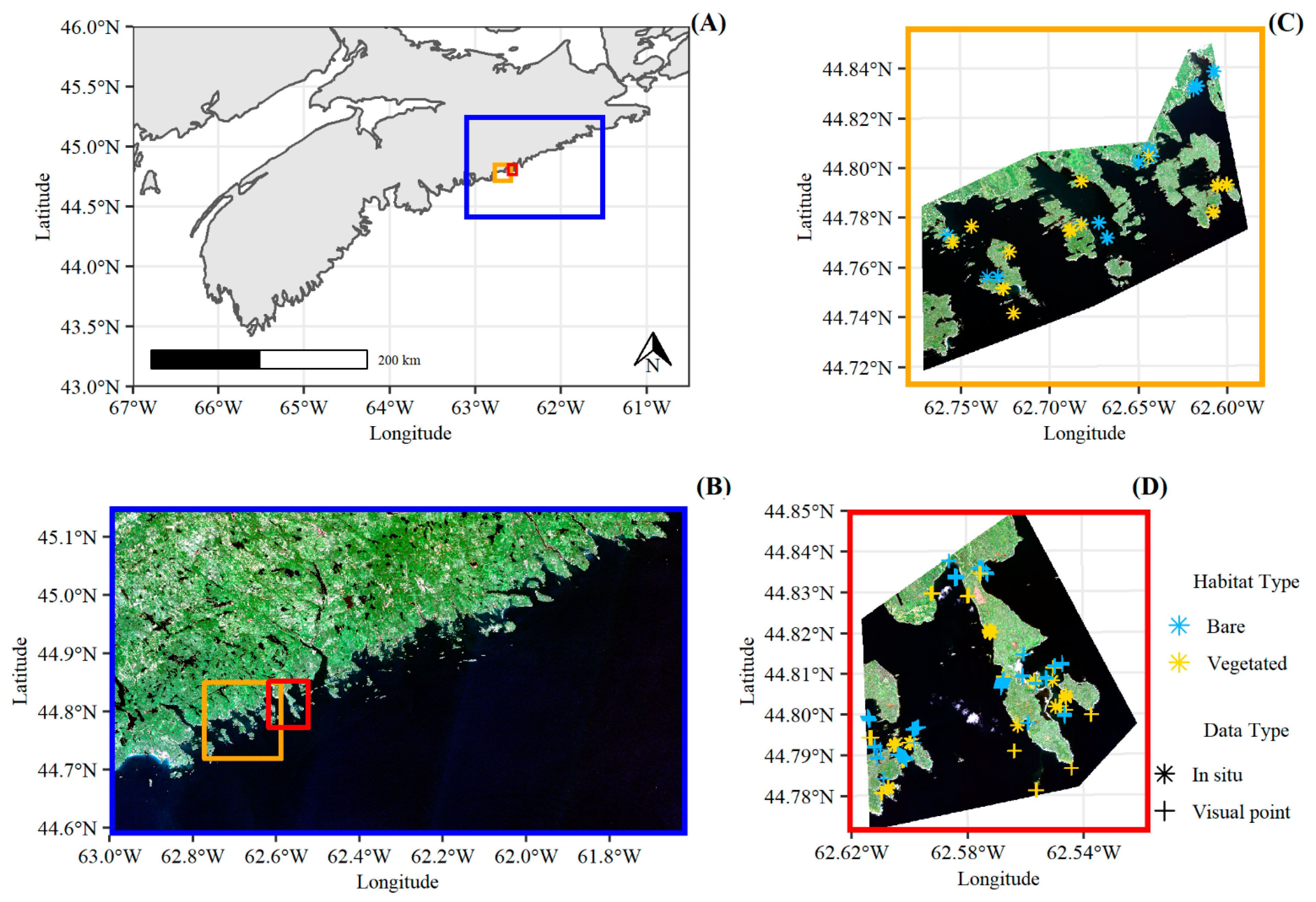
2.1. Study Area and Satellite Data

The Eastern Shore Islands along the exposed Atlantic Coast of Nova Scotia, Canada, are an ecologically and biologically significant area with large pristine marine macrophyte beds that include healthy eelgrass and kelp populations [32]. Water clarity in the region varies due to periodic wave action resulting in sediment resuspension events, and freshwater runoff with high concentration of CDOM and other particulate matter. Previous work has developed bottom habitat maps delineating the distribution of submerged aquatic vegetation (SAV) in this region using freely available Sentinel-2 imagery acquired on 13 September 2016 [31]. We used this bottom habitat map for comparison with WorldView-3 imagery in this study. Sentinel-2 imagery is available from the European Space Agency with four bands available at a 10-m spatial resolution, and images are acquired every 2–3 days at 45° N from two different satellites: Sentinel-2A and Sentinel-2B (Table 1) [33]. For the WorldView-3 imagery, two archived ortho-ready standard Level 2A WorldView-3 images were purchased over a subset of the region covered by the Sentinel-2 imagery (Figure 1). As in [34], we opted to use the WorldView-3 imagery in its native multispectral resolution of 2-m as the large bandwidth of the panchromatic band (0.3-m spatial resolution with 450–800 nm bandwidth) has limited water penetration. The first WorldView-3 image was acquired on 11 August 2019 at 12:17 ADT within five minutes of low tide (0.6 m) at 26.4° off-nadir (Table 1). The second WorldView-3 image was acquired on 17 August 2019 at 12:12 ADT at a higher tidal height (1.8 m) and 28.1° off-nadir. A small spatial overlap exists between the two images to allow for a comparison of tidal height impacts on classification success (Figure 1). The Sentinel-2 map, acquired three years before the WorldView-3 images, confirmed that the large-scale distribution (~100 km2) of marine macrophytes remained stable over the three-year period. It is worth noting that while we only examined WorldView-3 images in this study, we assume all conclusions are transferable to WorldView-2 imagery as these satellites have almost identical specifications. See Figure 2 for an overview of the methods described in the following sections.

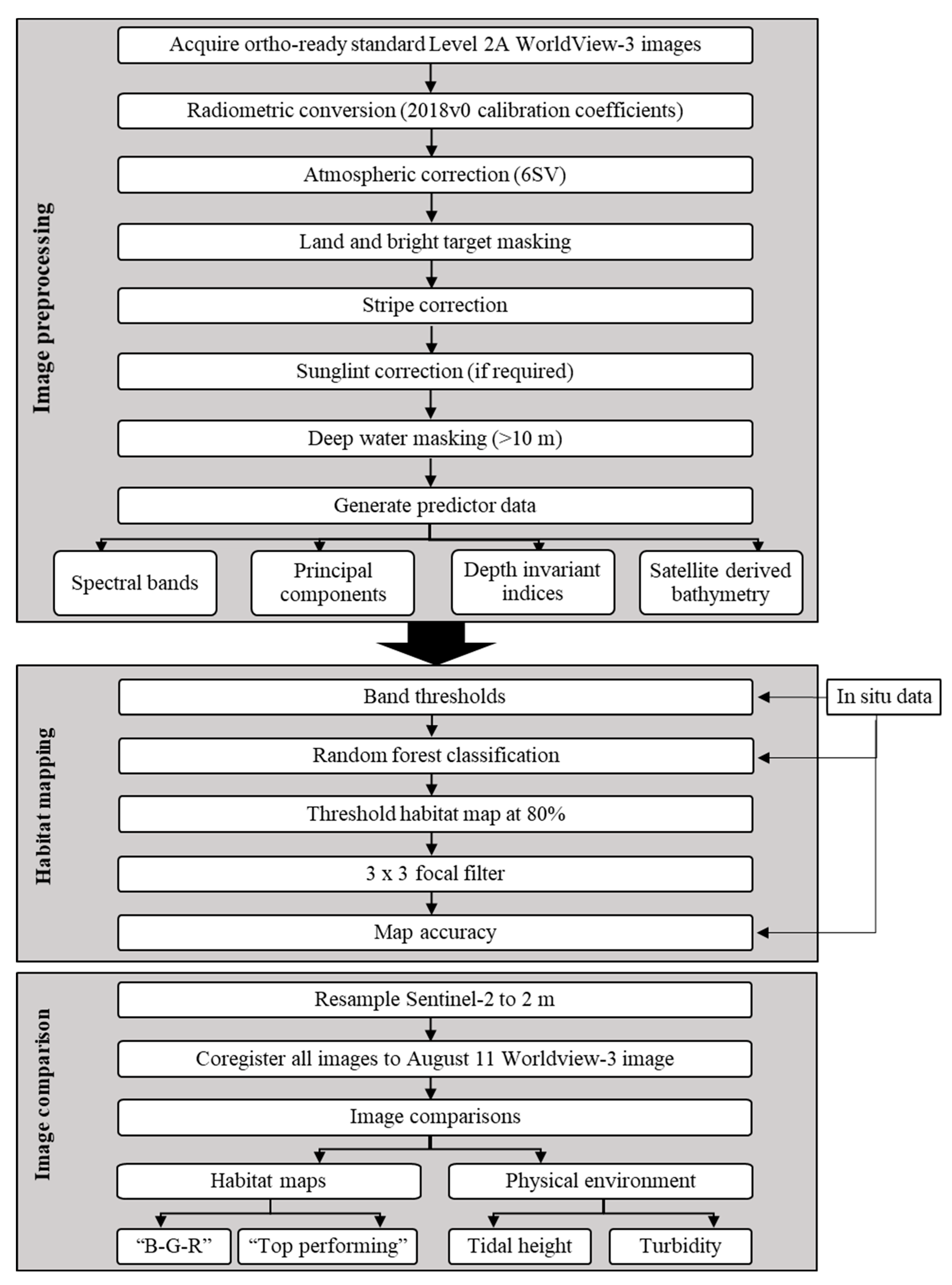
2.2. Image Preprocessing: WorldView-3 Atmospheric and Striping Correction

Standard Level 2A WorldView-3 products were provided as digital numbers and converted to top-of-atmosphere (TOA) reflectance using the 2018v0 calibration coefficients [37]. However, as also observed by [25], low reflectance values occurred over water targets due to the strong absorption of water which resulted in negative TOA reflectance values in the NIR bands after application of the calibration coefficients. Following a suggestion from the data provider (personal communication, 14 April 2020), the absolute value of the minimum negative TOA value produced following radiometric correction was added to all bands so the new minimum TOA value was set to zero. The added offset value differed between image dates but was the same for each band within an image.
TOA reflectance was converted to bottom-of-atmosphere (BOA) reflectance using the radiative transfer model 6SV [38]. In a comparison study to determine the best atmospheric correction scheme for WorldView-3 for bottom habitat mapping in the clear coastal waters of Spain, 6SV was found to have slightly superior performance than Fast Line-of-ight Atmospheric Analysis of Hypercubes (FLAASH) [39] and Atmospheric and Topographic Correction (ATCOR) [40] when compared to in situ measurements [41]. These results were in line with our own qualitative exploratory comparison of 6SV, FLAASH, Acolite [42,43] and dark object subtraction, where 6SV was also found to be the preferred atmospheric correction procedure, followed by Acolite (results not shown). To atmospherically correct the WorldView-3 images with 6SV, we set the atmospheric model to mid-latitude summer with a standard atmospheric pressure and a maritime aerosol model, and selected a Lambertian surface. To define the unknown aerosol optical thickness (AOT) at 550 nm, a polygon was defined over a homogenous region of optically deep water. We iteratively ran 6SV over a range of AOT for the red, red-edge, and NIR2 bands to find the highest AOT value which provided the lowest positive BOA values. This AOT value was then used as an input in 6SV to retrieve the aerosol signal and perform the atmospheric correction for all the visible bands. The NIR1 band was omitted from the AOT search as reflectance values for this band were significantly lower than all other bands, and suggested a significantly lower AOT to use than the other three bands. All land and other bright targets (e.g., breaking waves) were masked out of the imagery if any band surpassed a threshold for high reflectance values. These thresholds were defined based on their wavelengths where bands with centre wavelengths < 700 nm were masked on a threshold of 0.1 and bands with centre wavelengths > 700 nm were masked on 0.2. The increased threshold in longer wavelengths was to account for the stronger signal of vegetated habitat in these wavelengths when the canopy is near the surface. Areas of freshwater and clouds were manually masked.
Several vertical stripe artifacts were evident for most bands in the two WorldView-3 images (Figure 3). To correct for the stripes, we used a modified approach from the methodology described in [44]. We modified [44] to maintain our workflow within the R environment [45], as in [46]. As described in [44,46], stripes were identified in homogenous regions of the image, and an offset was calculated in these regions on opposite sides of the stripe. In contrast to [44,46], our approach does not require manual identification of stripes or offset regions. Instead, our stripe correction is a semi-automatic procedure once image specific input parameters of lag, peak distance, and peak height are specified (see Appendix A for a detailed methodological description). An example of the stripe correction is provided in Figure 2 and Supplementary Material Figure S8. Briefly, we looked for sharp changes in the mean value per column in the image (Figure 3C) and iteratively added or subtracted an offset from the widest stripe to eliminate the striping effect. This approach assumed every column contained optically deep water (or another region with homogenous habitat type), that the mean value of the optically deep water should be relatively constant across the image, and that stripes were represented by sharp transitions. While the final results still contained some artifacts (Figure 3B), the striping issue was drastically reduced from the initial image (Figure 3A).
The BOA de-striped bands (hereafter referred to as spectral bands) were then masked to exclude all pixels in water depths > 10 m using the same down-sampled bathymetry layer (Greenlaw Unpublished data), described in [31], to correspond with the maximum depth of ground-truthing points (see next section). A principal component analysis (PCA) was performed using the masked spectral bands one through six (coastal blue to red-edge) as a noise reduction, where the resulting principal components were used as predictor data in the map classification. The PCA removed some noise from both the water column and the WorldView-3 data. The spectral bands were also used in a water column correction based on depth invariant indices (DII) for bands one through five (coastal blue to red) [47]. A relative satellite-derived bathymetry (SDB) layer was created using the method in [48] with the blue and green spectral bands for the 11 August image only. Limited training data existed for the creation of the SDB band (n = 27), therefore no evaluation was performed and the layer was only used as a relative difference in water depth. We did not have enough depth points to create a SDB layer for the 17 August image. Both images were free of sun glint, therefore, no de-glinting step was required.

2.3. Habitat Mapping

To create the bottom habitat maps, we followed the same methods and used the same field data described in [31] to generate maps of vegetated bottom habitat extent. The field survey data was collected via drift drop camera surveys at predefined stations in September and October of 2019. An underwater video system was deployed for each station to ~1 m off bottom and observed bottom type was recorded as the system was allowed to drift for 1–2 min [31]. The coordinates and water depth were recorded for the start and end waypoints of the drift, with the occasional mid waypoint noted. In total, 96 stations were sampled over the Sentinel-2 tile, giving 218 data points. All data points were labelled as bare or vegetated habitat as previous work found that distinguishing between species type was not possible for Sentinel-2. Of the 96 stations, 26 overlapped the 11 August WorldView-3 image with 12 corresponding to bare habitat and 14 corresponding to vegetated habitat (predominantly eelgrass habitat). For the 17 August image, only 10 stations overlapped the imagery, all of which corresponded to vegetated habitat (predominantly eelgrass habitat). To supplement this limited data set, 17 stations were visually identified based on analyzing colour composites as non-vegetated habitat, and an additional 12 stations were identified as vegetated habitat. We made no attempt to distinguish between more habitat classes using the WorldView-3 imagery (i.e., eelgrass from various macroalgae species) due to the small sample size of our field survey data and the inherent difficulties in separating vegetation type with multispectral imagery.
As the WorldView-3 pixel size is smaller than Sentinel-2, and smaller than GPS accuracy (±3–5 m), and WorldView-3 water pixels in general were “noisier” then Sentinel-2 data, an additional processing step was performed on the field survey data. Small polygons were drawn around the location of the field survey point. These polygons were irregular to ensure only homogenous, continuous habitat patches were used for training. A set buffer distance (i.e., 5 m) was not used as the drift camera surveys often crossed habitat transitions. Instead, the tracks from the drop-camera drift surveys were used to inform where habitat transitions occurred in these irregular polygons. We did not omit these transitional habitat points in favour of buffering by a set distance as we had few field survey points to use. The respective satellite images were used as a basemap to inform the continuous habitat patches. Furthermore, to account for the high variability in reflectance values within a habitat type, each pixel extracted from these irregular polygons was considered an independent data point. These individual pixels were divided into training and testing groups during cross-fold validation described in the following paragraphs.
To generate maps of vegetated habitat extent from the WorldView-3 and Sentinel-2 imagery, we classified very shallow habitat (generally <2 m based on the downscaled bathymetry described layer in Section 2.2) with band thresholds for the normalized difference vegetation index (NDVI ≥ 0.3 as vegetated), which was calculated with the red and red-edge band, rather than the NIR band as in the Sentinel-2 classification. Next, shallow but non-vegetated habitat was classified with thresholds from the blue band (non-vegetated where blue ≥ 0.03 and 0.046, for 11 August and 17 August, respectively), and the red/green ratio (red/green ≤ 0.23 and 0.42, for 11 August and 17 August, respectively). These thresholds were set using information from field surveys. The remaining majority of pixels were then classified using a random forest classifier and the blue, green, and red bands as predictors with the augmented field survey information divided into five folds repeated ten times for repeated k-fold cross-validation for model development and validation. The final habitat map was produced by summing the number of times a pixel was classified as vegetation, divided by 50 (number of cross-validation runs), and converted to a percentage. The above methodology is the same that was employed to classify the Sentinel-2 imagery, with the exceptions of the specific threshold choices used in the band threshold calculations, and the use of the red-edge band in the NDVI calculation (Supplementary Materials Figure S1).
We additionally explored the full benefit of WorldView-3 data by comparing the effect of bottom habitat classification success with various input combinations of the visible spectral bands (omitting NIR1 and NIR2), principal components (testing PC1 through PC5), DII, and relative SDB bands [21,24,34]. A total of 12 combinations of visible spectral bands, with and without bathymetry, DII, and PCA were tested, from the simplest algorithm that used only three wavebands (3B), to the most complex model that included the six WorldView-3 visible bands, principal component analysis and depth invariant indices (6B-PC1-4-DII-SDB) (Table 2). Various combinations were tested to determine the top performing bottom habitat map classification. All random forest classifications were carried out using repeated k-fold cross-validation (five folds repeated ten times) to split the field data into training and validation groups.
As in the Sentinel-2 classification, all vegetated probability maps were thresholded using an 80% threshold of vegetated habitat probability. Previous work found this to be an optimal threshold to maximize overall accuracy [31]. In contrast to the Sentinel-2 classification, all WorldView-3 classifications were additionally subjected to a 3 × 3 focal filter to reduce salt-and-pepper noise in the classification. All analyses were performed in R version 4.0.4 (R Core Team, Vienna, Austria) [45] using the raster [49], RSToolbox [50], caret [51], pracma [52], readxl [53], and irr [54] packages.
To evaluate model performance, we used confusion matrices noting producer, user and overall map accuracy, and a kappa coefficient with z-tests for significance from zero [55], as also done to evaluate the Sentinel-2 classification [31]. We additionally generated F1 scores, a newer accuracy assessment approach that balances precision (user accuracy for the vegetation presence class) and recall (producer accuracy for the vegetation class) [56], as it is increasingly included in bottom habitat remote sensing studies [20,57,58]. All accuracy metrics presented are the average from the 50 k-fold cross validation runs. Yet, further evaluation was required to identify the top performing WorldView-3 classification given the relatively small differences in overall map accuracy, F1 scores, and kappa values across combinations (see Section 3). We additionally created an ensemble mean classification from all habitat maps and tested if (1) this ensemble mean habitat classification was most optimal or (2) if the highest performing classification could be defined as the individual classification which was most similar to the ensemble mean. We created the ensemble mean classification by taking the mean value per pixel of all tested habitat map classification and thresholding at 80%. We defined the most similar by looking at the mean absolute difference in vegetated habitat probability between the ensemble mean classification and each individual classification. We further visually examined all habitat classifications to see how they corresponded to the WorldView-3 true colour composites image and field survey points. Each criteria described here: confusion matrices, difference from ensemble mean, and visual examination, were used to define the top performing WorldView-3 habitat classification.

2.4. Image Comparison

We examined the differences in bottom habitat maps produced by Sentinel-2 and WorldView-3 imagery using two comparisons. First, we qualitatively confirmed that the broad scale habitat trends (e.g., location and general outline of large eelgrass beds) persisted across the three years. This first step was carried out because the field survey data and WorldView-3 imagery were both acquired in 2019, but the Sentinel-2 image was acquired in 2016. The Sentinel-2 map was resampled to a 2-m pixel size with the resulting 25 pixels retaining the same value as the original 10-m pixel. Second, the bottom habitat maps were co-registered to the 11 August WorldView-3 image, allowing a maximum shift of two Sentinel-2 pixels (~20 m) using the coregisterImages function in RStoolbox [50]. This method linearly shifts the image along rows and columns to maximize the amount of mutual information.
The first comparison examined the effect of the increased spatial resolution of WorldView-3 relative to Sentinel-2, independent of spectral resolution. The WorldView-3 images were classified the exact same way as the full tile Sentinel-2 map described in [31], using only the blue, green, and red bands, noted as “B-G-R” in text and figures. The second comparison examined the effect of both the increased spatial and spectral resolution of WorldView-3, where the top performing bottom habitat map classification developed in Section 2.2 was compared to the full tile Sentinel-2 classified image. To compare maps, we examined changes in overall coverage of vegetated surface area (SA) in the image, as well as on a per-pixel basis for the map classification.
It is important to note that while the methods used to classify the B-G-R WorldView-3 classification and full tile Sentinel-2 classification were the same, both images were classified on different training data and on different spatial extents. The Sentinel-2 image was classified at the level of the tile, using a set of field survey data that encompassed the entire region (n = 779). The WorldView-3 image was classified within a subregion of the Sentinel-2 image (Figure 1), using only the field data which overlapped with this subregion (n = 5330 and 6465 for 11 August and 17 August, respectively) that had been translated into polygon data to account for GPS inaccuracies. The higher number of validation points for the WorldView-3 images compared to Sentinel-2, despite the smaller area of interest, is due to the higher spatial resolution of WorldView-3. Due to the inherent differences in spatial extent and spatial resolution between the two sensors, we believe this is still a valid comparison as it is accounting for a typical use case for both sensors. Yet, for completeness, we also examined the impact on the comparison of the differences in spatial cover and training data. To do so, we reclassified the Sentinel-2 image using the exact same methods applied to the full tile classification [31], but on two different subsets. The first subset was based on cropping the Sentinel-2 image and Sentinel-2 training/testing data by the extent of the respective WorldView-3 images. This tested the effect of spatial extent. The second subset was also based on cropping the Sentinel-2 data to the WorldView-3 images, but used the same training/testing data as the respective WorldView-3 image. This tested for the effect of spatial extent and differences in training/testing data. We present the average overall map accuracy, kappa, F1 scores and habitat surface area coverage for the two Sentinel-2 subsets, but all maps reference the initial full tile Sentinel-2 habitat classification which was still the focus of our WorldView-3 and Sentinel-2 comparison as the ability to generate habitat maps across a 100 × 100 km is a strength of the Sentinel-2 data catalog.
Differences in the physical environment at the time scenes that were captured may also affect the accuracy of the resulting habitat map. We examined two parameters that would have differed between image acquisition dates: tidal height and turbidity. To examine how tidal height impacted classification success, we examined changes in predicted habitat extent across the three scenes where they overlapped. Satellite-estimated turbidity (T) was calculated using the method in [59]:
T = (Aλ × ρw(λ))/(1 − ρw(λ)/Cλ)
where ρw(λ) is the water leaving reflectance and Aλ and Cλ are wavelength-dependent calibration coefficients. This method uses a switching formula where turbidity is calculated using the red band when ρw(red) < 0.05 and using a NIR band when ρw(NIR) > 0.07. A blending algorithm is used for intermediate values:
T = (1 − w) × Tred + w × TNIR
where Tred is the turbidity calculated using the red band, TNIR is the turbidity calculated using the NIR band, and w is a weighted value:
W = (ρw(red) − 0.05)/(0.07 − 0.05)
Wavelengths and coefficients for both sensors are provided in Table 3. The 10 m depth contour is presented on all turbidity maps to indicate regions where optically shallow water impacts the water-leaving reflectance and derived turbidity, which should be treated with caution. Furthermore, we only examined relative differences as no in situ data were available for validation of absolute values for the turbidity algorithm (FNU). While we have tested for differences in spatial resolution, spectral resolution, spatial extent, training/testing data, tidal height, and water clarity between Sentinel-2 and WorldView-3, inherent differences in habitat classifications may still remain due to the variation in bandwidths across comparable bands, and the reduced signal to noise ratio of WorldView-3 relative to Sentinel-2.

3. Results

The differences in performance and resulting predictions between the 12 combinations of input parameters varied between the two WorldView-3 images, and no set combination consistently produced an accurate bottom habitat map across the entire image and depth gradient. The 11 August WorldView-3 image (mean depth of shallow habitat (<10 m) = 4.2 m) had very small differences in overall map accuracy, F1 score and kappa across the various input parameter combinations (Figure 4). Yet there were larger differences in predicted surface area with notable visual differences in the resulting bottom habitat maps (Figure 5). For instance, the classification built on just the depth invariant indices had the best bottom habitat delineation along the deeper edges of vegetated habitat, at the expense of over-classifying vegetation extent in shallower waters; whereas the classification built on just spectral bands classified the region highlighted in Figure 5 very well, but failed in other regions of the imagery, particularly on the eastern side in deeper water. The inclusion of the SDB layer was a strong driver of bottom habitat trends, with the resulting classification closely aligning with the SDB layer. Overall, it was difficult to assign a top performing classification to the 11 August image as all classifications largely failed on the eastern side of the imagery. In contrast to the 11 August image, the 17 August WorldView-3 image collected at high tide (mean depth of shallow (<10 m) habitat = 4.6 m) had the largest differences in overall map accuracy, F1 score and kappa between various input combinations, in particular for the combinations with reduced principal components (PC1-3 and PC1-2; Figure 4) with little corresponding visual differences in the resulting SAV maps (Figure 6); albeit even the largest differences were <5% different in accuracy metrics. As in the 11 August image, we found that the classification built only on the depth invariant indices produced the best habitat maps in deeper regions, with a high degree of misclassification in shallower waters. The classifications built on just the spectral bands had high map accuracies with a tendency to over-predict vegetated habitat. The classifications built on the principal components were a balance of the spectral bands and depth invariant indices, outperforming neither but balancing the limitations of each.
We analysed several parameters to define which was the highest performing WorldView-3 habitat map including map accuracy metrics (overall map accuracy, kappa, and F1 score), an ensemble mean habitat classification, and the difference in individual classifications from the ensemble mean classification. We opted to not use the ensemble mean habitat classification as trends were strongly driven by vegetation presence in any single classification, negating the success of a couple of classifications in specific regions (results not shown). However, when comparing the difference in an individual classification from the ensemble mean for the 17 August image, we found that, on average, the probability of vegetated habitat was within ~10% between most classifications and the ensemble mean (Supplementary Materials Figure S2); the exception being the classifications PC1-3 and PC1-2 which had larger differences. As such, for the 17 August image, the top performing bottom habitat classification was determined to be the one which included the six spectral bands, the first four principal components, and the depth invariant indices which maximizes the amount of data available to be used in the random forest classification. This bottom map classification produced a highly accurate (overall map accuracy = 99.8%; kappa = 0.99; F1 score = 0.99) map for the 17 August WorldView-3 image (Figure 4), that closely aligned with trends visible in the true colour composite (Figure 6), and predicted relatively low differences in vegetated habitat probability from the ensemble mean classification (Supplementary Materials Figure S2).
For the 11 August image, there was more variation between the mean absolute difference in vegetated habitat probability between the ensemble mean classification and each individual classification (Supplementary Materials Figure S2). This was consistent with our finding that there was more variation in classified habitat maps across predictor combinations for this image date. For the single classifications with lower differences compared to the ensemble mean classification, on average, the probability of vegetated habitat was within ~10–15%. These classifications included the six spectral bands (6B), principal components (PC1-5, PC1-4), all predictor variables, and the more refined predictor classifications (BG-PC12-SDB). As such, we found the latter classification with the first two principal components, blue and green spectral bands, and the SDB layer to be the top performing bottom habitat classification (overall map accuracy = 99.9%; kappa = 0.99; F1 score = 0.99; Figure 4). This combination was most accurate along the eastern side of the imagery, with some compromises on classification success in other regions of the imagery (Figure 5), and had relatively low differences from the ensemble mean (~12%; Supplementary Materials Figure S2). Here, the combination of the first two principal components helped to provide de-noised data into the classification, with the most water penetrating spectral bands (blue/green), delineating extra information that may be lost in the PCA.
Differences in spectral signatures between bottom habitat types varied between the WorldView-3 and Sentinel-2 sensors, yet the nature of these differences depended on the number of spectral bands considered (Figure 7). For Sentinel-2, differences in spectra between vegetated and non-vegetated habitat were observed as a change in magnitude rather than shape, with fragmented/patchy habitat presenting as intermediate reflectance values. When we extracted the spectra for all WorldView-3 pixels corresponding to one Sentinel-2 pixel (Figure 7A,C,E), we saw a large range of variation in spectra for the patchy habitat as the smaller pixel sizes are more likely to encompass a region of homogenous habitat type with less mixing within an individual pixel. Similar to Sentinel-2 when only the blue, green and red bands were considered, the differences in spectra for habitat types with WorldView-3 imagery were largely a change in magnitude of reflectance with similar spectral shape. The reflectance values for the red and green bands were very similar between the two sensors despite the three-year difference between images and variations in water column properties. Yet, the blue Sentinel-2 band was systematically lower than the WorldView-3 blue band across all habitat types. When all six WorldView-3 bands were considered (Figure 7B,D,F), there were differences in spectral magnitude and shape across the three habitat types. The information captured by the WorldView-3 band 6 (red edge) is noteworthy, as the reflectance in that band increased in the presence of vegetation in shallow depths, while continuing the decreasing trend from adjacent bands over sandy bottom.
The increased spatial resolution of WorldView-3 (2-m) alone produced improved bottom habitat maps compared to Sentinel-2 (10-m). Regardless of input parameters, the WorldView-3 classifications trained using only the blue, green, and red bands (B-G-R), and the same methods as the Sentinel-2 classification always had a higher overall map accuracy (>94%; Figure 4), kappa (>0.99) and F1 score (>0.99) than the Sentinel-2 classification (Figure 8). It is important to note the magnitude of differences in accuracy statistics between sensors decreases as the spatial extent of the Sentinel-2 habitat map is reduced, and the difference in training/testing data is removed. As such, the accuracy improvements for WorldView-3 are likely a combination of the smaller spatial scale, and the reduced pixel size. Nevertheless, both sensors were able to classify bottom habitat well to the 10 m depth contour. However, there were some reductions to this maximum depth in parts of the imagery where transparency is reduced, and some limitations across all depths on the eastern side of the 11 August WorldView-3 image.
We further explored how the surface area (SA) of each habitat type differed for the overlapping area between the Sentinel-2 map and the two WorldView-3 images (Figure 1B). Total vegetated SA differed by ~25% and ~20% for the 11 August and 17 August WorldView-3 images, respectively (Figure 8). The difference in SA was evenly split between Sentinel-2 classifying a region as bare while WorldView-3 classified the same area as vegetated, and vice versa, for both WorldView-3 images. While Sentinel-2 and both WorldView-3 images captured the general pattern of vegetated presence, the impact of the increased spatial resolution was very clear in the WorldView-3 habitat maps, with much more accurate bed delineation (Figure 9 and Figure 10), in particular along bed edges. For instance, if we divide the highlighted area in the 17 August map in Figure 9 along selected depth contours (i.e., 3, 7 and 10 m), the most differences occur between the 3 and 7 m depth contour with more fragmented habitat types identified by the WorldView-3 image. Within this depth contour, about 40% of pixels differed between the two classifications where the Sentinel-2 image was classified as vegetated, but bare in the WorldView-3 image. Interestingly, both shallow (<3 m) and deep (>7 m) regions had greater agreement between sensors, with ~20% of pixels differing between the two classifications. For the 11 August image, fragmented eelgrass habitat existed across depth gradients and all three contour groups differed by ~30% of the pixels between Sentinel-2 and WorldView-3 (Figure 10). For this 11 August comparison, WorldView-3 was more likely to classify a pixel as vegetated. Lastly, we explored if our choice of threshold (80%) had an impact on the predicted vegetated SA (Supplementary Materials Figure S3). We found that the differences in SA between the Sentinel-2 and B-G-R WorldView-3 classifications could be decreased with a different choice of threshold (Supplementary Materials Figure S3).
Increased WorldView-3 spectral and spatial resolution improved habitat delineation, but with only minor improvements in accuracy and small changes in vegetated SA (Figure 9 and Figure 10). The overall map accuracy marginally improved by ~0.4% from 99.4% to 99.8% for the 17 August WorldView-3 image, with little change in total SA of predicted SAV habitat for the top performing classification (Figure 8). The full tile Sentinel-2 and top performing 17 August WorldView-3 classification were most similar (10% of pixels differing) at shallow depths (<3 m), and all classifications had a similar amount of differing pixels at greater depths (Figure 9). For the 11 August image, there was no change in overall map accuracy from the “B-G-R” classification to the top performing classification. However, the percentage of differing pixels relative to the full tile Sentinel-2 classification across the entire image increased from ~25% to ~30%. Two-thirds of the disagreements between sensors were pixels classified as vegetated by WorldView-3, and bare by Sentinel-2 (Figure 8). There was spatial variation in the distribution of mismatched pixels across depths for the 11 August image (Figure 10). For both image dates, a threshold of ~80% produced a total vegetated SA that was closest to the Sentinel-2 vegetated SA (Supplementary Materials Figure S3).
When examining differences in the physical environment across the images, we found that for the WorldView-3 images, tidal height had little impact on classification success (Figure 11). Contrary to expectations, the higher tidal height 17 August image produced the most accurate bottom habitat map relative to 11 August and the full tile Sentinel-2 image. This is likely due to differences in water clarity which changes on short time scales in coastal waters. Turbidity values were highest (2.64 ± 0.93 FNU; mean ± SD) for the 11 August WorldView-3 image (Supplementary Material Figure S4), slightly less (2.13 ± 0.40 FNU; mean ± SD) for the WorldView-3 17 August image (Supplementary Material Figure S5), and lowest for the full tile Sentinel-2 image (1.61 ± 0.47 FNU; mean ± SD). Thus, the WorldView-3 image date with the lowest turbidity values (17 August) produced the best habitat map, despite being acquired at a much higher tidal height. Within only the area that overlapped across all three images, the 17 August image was most similar to the full tile Sentinel-2 classification, with only ~18% of pixels differing compared to ~22% for the 11 August image and <4% percent difference in vegetated SA (Supplementary Material Figure S6). Interestingly, when the high tide image (17 August) was compared to the two low tide images, the 17 August image was most different to the full tile low tide Sentinel-2 image at shallow depths (0–3 m), but most different to the low tide 11 August image at moderate depths (4–7 m). There was little difference between all classifications at deeper depths (7–10 m).

4. Discussion

Mapping bottom habitat with high resolution satellite imagery is increasingly being used to identify, quantify and monitor coastal vegetated habitats. However, there are important considerations in sensor choice to accurately define such habitats. We created a robust methods workflow to map bottom habitat in an optically complex temperate environment using the eight bands of the WorldView-3 sensor. We explored various atmospheric correction and image preprocessing steps to identify a top performing classification scheme for the WorldView-3 sensor in our area of interest. Our preprocessing workflow (atmospheric correction, stripe correction) has been adapted to be robust and semi-automatic which can readily be applied to any image date. However, the exploration of predictor data combinations is a hands-on, time intensive task, particularly when using the random forest classification, which is an image-based approach that must be retrained for every image date. After identifying an optimal methods workflow for WorldView-3 imagery, we compared habitat maps produced by freely available Sentinel-2 imagery at 10-m resolution, to habitat maps produced from 2-m WorldView-3 imagery. Such comparisons can inform the design of coastal monitoring programs to understand the benefits of each sensor considering differences in their spatial and spectral resolutions, available data catalogues, image footprints, and cost of image acquisition; particularly as imagery such as Sentinel-2 generally has more support from the scientific community towards the development and validation of algorithms, typically with free open-source tools.

4.1. Generating WorldView-3 Habitat Maps

While determining the top performing WorldView-3 classifications using a random forest algorithm, we found combining different input parameters (e.g., number of bands, bathymetry) improved our classification success, particularly when combining a principal component analysis on the spectral bands with different combinations of spectral bands. In contrast, other studies based on WorldView-3 images have successfully mapped bottom habitat using only the information from spectral bands [15,16,22,63,64]. In general, these studies used some combination of bands one (coastal blue) through six (red edge), and only employed the NIR bands for removing glint. Our exploration of the six spectral bands found the most important information came from bands two (blue) through five (red), which was also observed by [65]. Other data that has been used to train supervised classifiers in WorldView-3 bottom habitat mapping studies include water column corrected bands [65,66,67,68], principal components [69], or hybrid combinations of the aforementioned parameters, including spectral bands [24,34] and remotely sensed data acquired from Lidar or acoustic sensors [16]. In agreement with other WorldView-3 studies that directly compared bottom habitat maps produced from different input data, we found maps produced from only water column corrected bands were outperformed by maps produced from either spectral bands [34,70] or principal components [71,72]. When comparing between principal components and spectral bands, marginal increases in classification success have been observed for the principal components [34,72]. We found that principal components produced habitat maps which were less “salt-and-peppered” than the spectral or depth invariant (water column corrected) maps, yet they did not necessarily outperform the habitat maps produced with only spectral bands. Thus, the principal components were useful for noise reduction. Only one other study has tested classification success using random forest with spectral bands, principal components, depth invariant indices, and bathymetry for bottom habitat mapping with WorldView-3 imagery specifically and they found that de-glinted spectral bands produced the best habitat maps with insignificant increases in map accuracy when all data was used [24]. Interestingly, in our study, we had different conclusions depending on which image was examined. The first WorldView-3 image acquired on 11 August had insignificant differences in map accuracy regardless of input data, with large visual differences in the resulting habitat map (up to 20% difference in SA estimates). We found the opposite for the second WorldView-3 image acquired on 17 August; there were larger differences in map accuracy with little visual change in the resulting habitat map. As such, we concluded in general it was best to use all input data to train the random forest algorithm to provide the highest amount of data for model training. Such approaches have been used to map bottom habitat with other satellite imagery such as Sentinel-2 [21]. Yet, if suboptimal habitat maps are produced, such as in the 11 August image, further exploration is still required to find the combination of input data which produces the best habitat map.
The top performing habitat map produced for the 11 August image still largely failed to properly classify the bottom habitat on the eastern side of the imagery. This poor performance may be due to an incomplete stripe correction as reflectance values were highest on the eastern side of the imagery. Stripe artifacts have negatively impacted other bottom habitat mapping projects [70], yet we could find only two other studies which discussed stripe correction for WorldView-3 imagery [44,46]. The high reflectance values may also be indicative of differences in water clarity across the image as the highest turbidity values were observed in this area across all three image dates. While satellite-estimated turbidity has not typically been done using WorldView-3, it has been successfully performed and validated using Sentinel-2, e.g., [73,74]. Turbidity values were likely elevated by a moderate rainfall event on August 8, 2019, three days before the first WorldView-3 image was collected [75]. Such events can reduce water clarity in coastal regions due to terrestrial run-off. When the true colour composites were examined, dark river plumes were evident in the 11 August image (Supplementary Materials Figure S7), and not in the 17 August or Sentinel-2 image, indicating water clarity improved during the six days between image acquisition. Additionally, the systematic lower reflectance in the blue band for the Sentinel-2 image suggests varying water optical properties across image dates, likely due to varied CDOM (colored dissolved organic matter) concentrations. However, this difference may also result from an incomplete atmospheric correction for the WorldView-3 imagery, such as over correction of the Rayleigh (i.e., molecular) or aerosol signal. As such, we found that both the poor radiometric calibration and changes in water clarity had a greater impact on classification success than tidal height. The high tidal height in the 17 August image produced a more accurate habitat map in the region of overlap with the low tidal height of the 11 August image. The high tide 17 August and low tide Sentinel-2 images both had much lower turbidity values than the low tide 11 August image. This has important implications for bottom habitat mapping projects with WorldView-3 imagery as image catalogs are limited and expensive, and the best image for habitat mapping may not be the one at the lowest tidal height but rather the one with the highest transparency.
An additional benefit of WorldView’s increased spatial and spectral resolution is the potential to map bottom habitats more precisely with differentiation between vegetation types (e.g., for instance, separating eelgrass from seaweed). On Canada’s West coast, WorldView-2 imagery was used for separating eelgrass from brown and green seaweeds to a maximum depth of 3 m [16]. In other turbid waters in Europe, WorldView-2 was used to distinguish between various submerged aquatic vegetation types to a maximum depth of 2 m [15]. In regions with clearer water, WorldView-3 has been used to differentiate between corals, seagrass, and seaweed habitats to greater depths (<20 m) [22,24]. Unfortunately, we lacked sufficient field survey information to test species-type habitat mapping with the WorldView-3 imagery. Species-type habitat mapping with WorldView-3 imagery will be explored in the future where our objective is to separate eelgrass from various seaweed species.

4.2. Comparing Sentinel-2 and WorldView-3

We found the full benefit of the WorldView-3 bottom habitat maps came from both the increased spatial and spectral resolution. Compared to the “B-G-R” three band (blue, green, red) WorldView-3 habitat maps, defining a top performing classification that made use of the full spectral resolution of WorldView-3 improved bed delineation. In the clear waters of the Mediterranean Sea, seagrass habitat maps produced by all four 10-m Sentinel-2 spectral bands (blue, green, red, and NIR) were compared to maps produced with 8-band (including both NIR bands), and 4-band (blue, green, red, and NIR) WorldView-2 imagery [8]. Similar overall map accuracy values were observed for the 4-band WorldView-2 maps, relative to the 8-band maps (~96–97%), with a slight reduction in accuracy for the Sentinel-2 maps (~93–97%). Overall, the authors concluded that WorldView-3 is the better sensor for seagrass habitat mapping, but Sentinel-2 is adequate if precise delineation of beds is not required [8]. Elsewhere in the Mediterranean Sea, depth invariant indices were used to map seagrass habitat with WorldView-2 and Sentinel-2 imagery [30]. Higher map accuracy values were also observed for the WorldView-3 imagery, although both images were capable of mapping general seagrass trends (differences in accuracy were ~≤11%). Similarly, in the shallow (<3 m) water off Eastern Banks in Australia, seagrass maps were produced using three 10-m spectral Sentinel-2 bands (blue, green, red) and five 2-m WorldView-3 bands (coastal blue through to red) [29]. Both sensors delineated similar seagrass habitat maps, with WorldView-3 based habitat maps providing more detail and slightly higher overall map accuracy values relative to the Sentinel-2 based classification (<5% difference). Consequently, our findings in a temperate region with optically complex water are consistent with other regional studies where both WorldView-3 and Sentinel-2 were used to map vegetated coastal habitat. WorldView-3 imagery allows for a marginally higher degree of accuracy and better bed delineation, and Sentinel-2 readily allows for habitat mapping over large spatial scales. Furthermore, estimates of vegetated SA extent may further agree across sensors (Sentinel-2 vs. WorldView-3) if image acquisition dates were close to each other (i.e., within a year), opposed to only the same season but three years apart as currently analyzed. The selected 2016 Sentinel-2 image was the optimal image within the Sentinel-2 data catalog for bottom habitat mapping as it was cloud-, glint- and wave-free, with relatively clear waters at a low tidal height [31]. No 2019 Sentinel-2 image matched these quality criteria, with the only potential images being impacted by sun glint, which has detrimental impacts on bottom habitat classification success. Nevertheless, while the coarse, broad scale habitat distribution remained stable from 2016 to 2019, it is possible that some differences in habitat classification are exclusively due to changes in fine scale habitat extent over the three-year period (e.g., changes in percent cover, shifts in distribution of fragmented habitat), and poorer agreement of the Sentinel-2 data to the 2016 field data, rather than inherent differences between the two sensors.

5. Conclusions

In this study, we first created a methods workflow to classify WorldView-3 imagery from digital numbers to bottom habitat maps in a temperate, optically complex environment. The preprocessing steps (including atmospheric correction and destriping) have been designed to allow for semi-automatic processing of many images with little manual input. However, the random forest classification requires image specific training and validation. We then tested how the WorldView-3 bottom habitat maps produced at a 2-m resolution compared to a bottom habitat map produced from Sentinel-2 at a 10-m resolution. We demonstrated that both Sentinel-2 and WorldView-2/3 are capable of mapping bottom habitat in a temperate optically complex environment. The top performing WorldView-3 classification which made use of WorldView-3 increased spatial and spectral resolution best delineated the high spatial heterogeneity of the Eastern Shore Islands, but both sensors accurately outlined the major vegetated beds. Sentinel-2 provides global, freely available imagery at a 10-m spatial resolution with three water penetrating bands. The large image catalog is readily available, which allows for monitoring and quantification of changes in vegetation extent at large spatial scales. In contrast, WorldView-2/3 imagery must exist in archives, or be specifically tasked for an increased cost, but can delineate specific macrophyte beds precisely if adequate attention is paid to radiometric quality. While three more water penetrating bands are available for image classification, classification is reliant on a single image which is problematic if there are image quality issues (poor water clarity, stripe artifacts, haze, etc.). Given the benefits and limitations of each satellite sensor, we provide two recommendations on the use of satellite remote sensing to map and monitor bottom habitat in Atlantic Canada and regions with similarly optically complex coastal waters. Firstly, for large-scale mapping (e.g., Atlantic coast wide, >100 km2), we would recommend the use of Sentinel-2 as it provides a cost-effective means of mapping the large-scale trends in vegetated habitat extent. For small-scales areas (e.g., single bays or beds) where highly accurate mapping is required (e.g., delineation of eelgrass beds within MPAs), we recommend using WorldView-2/3 with special care taken to ensure data quality. WorldView-3 has the advantage of additional bands to detect bottom habitat, which advocates for the use of hyperspectral data to derive bottom habitat maps, including species differentiation, with greater success. While the addition of bands is useful, spatial resolution remains a key parameter, in particular when vegetation is fragmented and located in complex spatial environments, such as the Eastern Shore Islands, Nova Scotia, Canada. Its high spatial resolution can also support many marine spatial management questions that require a fine spatial resolution such as the placement of aquaculture nets over eelgrass beds. Marine macrophyte beds provide crucial ecosystem functions and services in coastal habitats, and Sentinel-2 and WorldView-3 imagery are valuable tools to quantify their distribution over various spatial scales.

Supplementary Materials

The following supporting information can be downloaded at: https://www.mdpi.com/article/10.3390/rs14051254/s1, Supplementary Material 1. Figure S1: Methods workflow to classify the Sentinel-2 imagery, modified from [31]. White boxes are identical steps between the Sentinel-2 and Worldview-3 imagery. Red boxes are where there were some differences between the classifications. Figure S2: Mean absolute difference (+standard deviation) of vegetated habitat probability for the ensemble mean Worldview-3 classification relative to each habitat classification prior to image thresholding for the August 11 Worldview-3 image (A) and August 17 Worldview-3 image (B). Figure S3: Impact of threshold choice on the percent difference in vegetated surface area between the Sentinel-2 and August 11 Worldview-3 image (A) and Sentinel-2 and August 17 Worldview-3 image (B). The 80% threshold used in this study is indicated by the vertical dashed line. Figure S4: Turbidity (FNU) for the 13 September 2016 Sentinel-2 image versus the 11 August 2019 Worldview-3 image. Histogram for the Sentinel-2 (A) and Worldview-3 (B) and their respective maps (C,D). The percent difference in turbidity values (%) between the two image dates as a histogram (E) and map (F). The 10 m depth contour (black line) indicates regions of optically shallow water. Note that absolute turbidity values have not been field validated. Figure S5: Turbidity (FNU) for the 13 September 2016 Sentinel-2 image versus the 17 August 2019 Worldview-3 image. Histogram for the Sentinel-2 (A) and Worldview-3 (B) and their respective maps (C,D). The percent difference in turbidity values (%) between the two image dates as a histogram (E) and map (F). The 10 m depth contour (black line) indicates regions of optically shallow water. Note that absolute turbidity values have not been field validated. Figure S6: Percent difference in vegetated surface area (%) for the area that overlaps all image dates for various depth classes (0–3, 3–7, and 7–10 m) and for all depth classes together (0–10 m). Figure S7: True colour composite showing impacts of one river plume in the August 11, 2019 Worldview-3 image (A) which is absent in the 13 September 2019 Sentinel-2 image (B). Land (light grey) is masked in both images. Figure S8: Step by step example of the stripe correction using the red band for the 17 August 2019 Worldview-3 image: Generating the column mean value before (orange line) and after masking (black line) based on the 85% quantile, and indicating the column limits that were included in the stripe detection. Purple box denotes the zoom on panels C and D (A). Calculating the lagged difference between 30 column means to define the location of stripes based on the difference exceeding the peak height threshold and peak distance. Stripe edges are denoted with dashed lines, and stripes by alternating grey shades. The reference signal (widest stripe) is indicated with red shading and is the fifth stripe (B). A zoom in on the reference signal column mean indicating which values were used to calculate the offset value (grey shading). The offset value is added to each column mean within the adjacent stripe to generate the nonadjusted destriped column mean (red line) (C). The offset value was linearly adjusted over the column index where the stripe edge occurs (grey shading) to remove the spike in column mean over this small interval (D).

Author Contributions

Conceptualization, M.C.W. and E.D.; Methodology, K.L.W.; Writing—Original Draft Preparation, K.L.W.; Writing—Review and Editing, M.C.W. and E.D.; Funding Acquisition, M.C.W. and E.D. All authors have read and agreed to the published version of the manuscript.

Funding

This study was funded by the Fisheries and Oceans Canada Strategic Program for Ecosystem-Based Research and Advice (SPERA) and from in-kind support from the Oceans and Coastal Management Division, Ecosystem Management Branch.

Data Availability Statement

Publicly available and restricted datasets were analyzed in this study. The publically available Sentinel-2 data can be found here: https://scihub.copernicus.eu/ (accessed on 18 December 2021). Restrictions apply to the availability of WorldView-3 data which can be obtained directly from MAXAR. Field survey data can be shared upon request. Derived habitat maps and R code to implement all processing steps are available from the following GitHub repository: https://github.com/BIO-RSG/WorldView3_Sentinel_Comparison_Project.

Acknowledgments

We thank J. O’Brien and B. Roethlisberger for support in the field and laboratory. We thank A. Hilborn and J. O’Brien for reviewing the manuscript. We also thank the European Space Agency for freely providing Sentinel-2 data.

Conflicts of Interest

The authors declare no conflict of interest.

Appendix A

The stripe correction, coded in R version 4.0.4 [45], was implemented per band as follows:
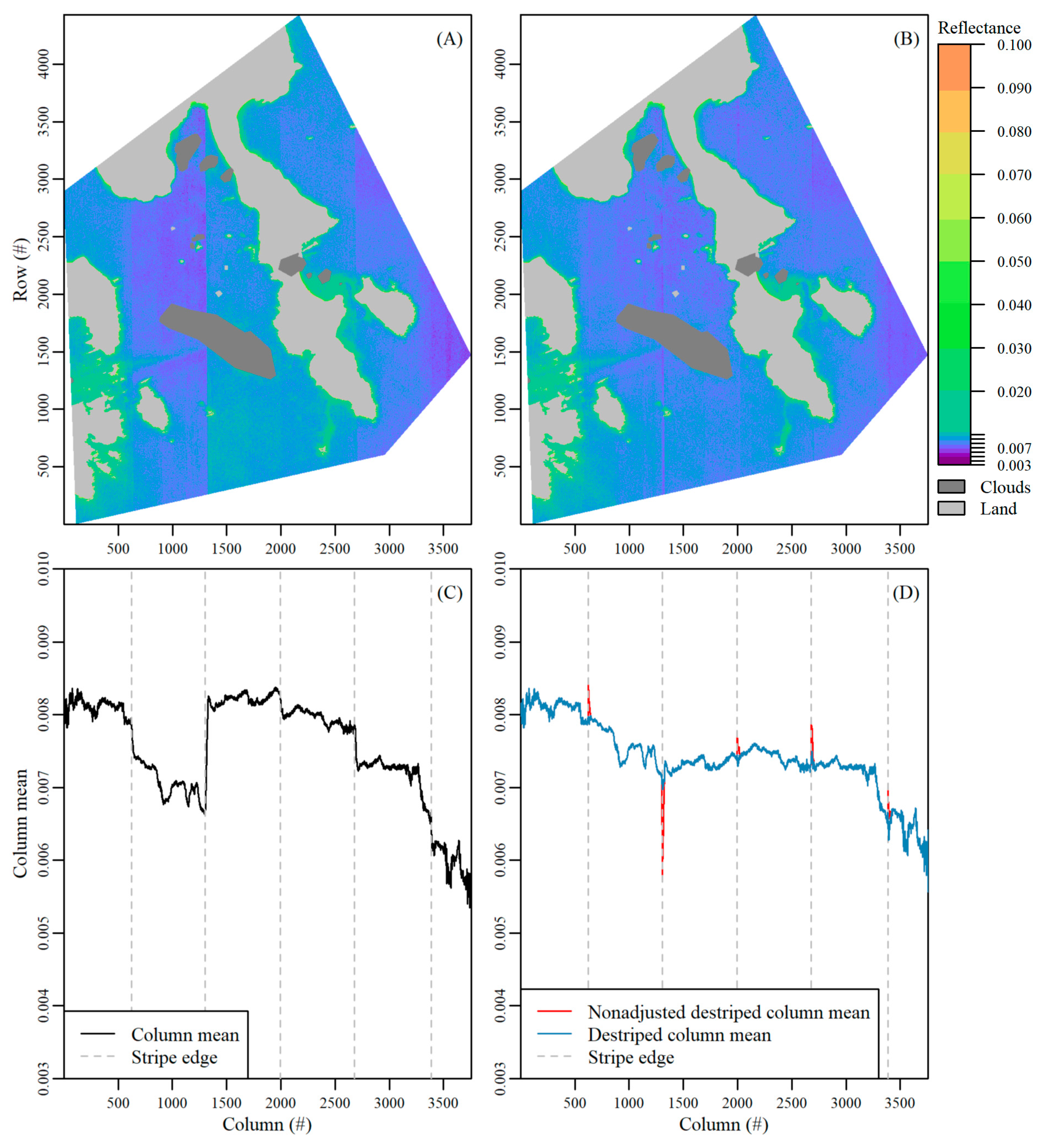
  • The mean value per column in the image (column mean) was determined, after masking and excluding bright pixels defined as greater than the 85% quantile of BOA reflectance values over the entire image (Supplementary Material Figure S8a). The bright pixels, which corresponded to nearshore areas where bottom reflection was not negligible, had a large effect on the initial mean column value and created many artificial peaks. Next, columns at the image edges were also masked, as they contained fewer valid rows which resulted in artificial peaks in the column mean values. In this study, we masked the first and last 50 columns for the 11 August image and the first and last 110 columns for the 17 August image. The number of columns was an image-specific number that is dependent on the area of interest, viewing and sun geometry.
  • Next, the difference between column mean values following a horizontal (column-wise) lag between columns was calculated (Supplementary Material Figure S8b). An appropriate lag number was image specific. In this study we used lags of 12 and 30 for the 11 August and 17 August images, respectively. The lag was required as stripe edges were not abrupt, but rather spread over a small range of columns, and a stripe may be missed if the difference was calculated only in the adjacent column mean. Next, we found the column index where there were sharp changes in the lagged differences in column means using the findpeaks function in the R package pracma [52]. This column index indicated the edges between various stripes. Sharp changes were defined by setting image specific thresholds for minimum peak height (i.e., minimum difference amount) and distance (i.e., minimum number of consecutive columns). In this study, we set minimum peak height to 0.0002, and 0.0003 for the 11 August and 17 August images, respectively, and peak distance to 500 columns for both images. Note, in Figure S8b, not all spikes above the peak height threshold were identified as a stripe edge as they were closer together than the minimum peak distance allowed. Defining accurate peak height and peak distance thresholds was critical for an accurate stripe edge detection. Lastly, the reference signal to which all other stripes were corrected to was defined by identifying the widest stripe. This arbitrary selection did not impact the habitat classification results as we additionally tested using the first and last stripe as reference with no impact on results.
  • Working horizontally outward from the reference signal, an offset value to correct the stripe effect was calculated (Supplementary Material Figure S8c). The importance of the lag in step 2 (see Supplementary Material Figure S8b) was highlighted here. While the stripe edge was identified at column 2675, there was a gradual decline in the column mean value until approximately column 2700 where the column mean became stable. For this same reason, the offset was calculated for a small number of columns away from the stripe edge where the column mean was relatively stable. To do so, the mean of column means for a small subset of columns on opposite sides of the stripe location was calculated. For both images, we took the mean of 10 columns, 40 columns to the left and right from the stripe edge (grey shading in Supplementary Material Figure S8c). The difference between these two means of column means (i.e., difference between reference signal and adjacent signal) were then calculated and added as an offset to all columns within the adjacent stripe. This step was incrementally repeated, working outwards from the reference stripe. Lastly, the masked columns at the scene edges (see Step 1, Supplementary Material Figure S8a) were corrected using the adjacent offset value for the outermost stripes.
  • There was over/under correction at stripe edges as stripes gradually transitioned over a small range of image columns. An adjustment was made to the offset value over this range (grey shading Supplementary Material Figure S8d). To do so, we linearly interpolated from the initial to the new offset value for the stripe over the range of columns in which the jump occurs so the offset value was incrementally changed (Supplementary Material Figure S8d). A final vector of offset values was thus created and added to the corresponding image columns to de-stripe the entire image.
  • Finally, these steps were applied to each band per image.

References

  1. Barbier, E.B.; Hacker, S.D.; Kennedy, C.; Koch, E.W.; Stier, A.C.; Silliman, B.R. The value of estuarine and coastal ecosystem services. Ecol. Monogr. 2011, 81, 169–193. [Google Scholar] [CrossRef]
  2. Wong, M.C.; Kay, L.M. Partial congruence in habitat patterns for taxonomic and functional diversity of fish assemblages in seagrass ecosystems. Mar. Biol. 2019, 166, 46. [Google Scholar] [CrossRef]
  3. Schmidt, A.L.; Coll, M.; Romanuk, T.N.; Lotze, H.K. Ecosystem structure and services in eelgrass Zostera marina and rockweed Ascophyllum nodosum habitats. Mar. Ecol. Prog. Ser. 2011, 437, 51–68. [Google Scholar] [CrossRef] [Green Version]
  4. Wong, M.C.; Dowd, M. A model framework to determine the production potential of fish derived from coastal habitats for use in habitat restoration. Estuaries Coasts 2016, 39, 1785–1800. [Google Scholar] [CrossRef]
  5. Teagle, H.; Hawkins, S.J.; Moore, P.J.; Smale, D.A. The role of kelp species as biogenic habitat formers in coastal marine ecosystems. J. Exp. Mar. Bio. Ecol. 2017, 492, 81–98. [Google Scholar] [CrossRef]
  6. Duarte, C.M.; Losada, I.J.; Hendriks, I.E.; Mazarrasa, I.; Marba, N. The role of coastal plant communities for climate change mitigation and adaptation. Nat. Clim. Chang. 2013, 3, 961–968. [Google Scholar] [CrossRef] [Green Version]
  7. Duffy, J.E.; Benedetti-Cecchi, L.; Trinanes, J.; Muller-Karger, F.E.; Ambo-Rappe, R.; Boström, C.; Buschmann, A.H.; Byrnes, J.; Coles, R.G.; Creed, J.; et al. Toward a coordinated global observing system for seagrasses and marine macroalgae. Front. Mar. Sci. 2019, 6, 317. [Google Scholar] [CrossRef] [Green Version]
  8. Marcello, J.; Eugenio, F.; Gonzalo-Martin, C.; Rodriguez-Esparragon, D.; Marques, F. Advanced processing of multiplatform remote sensing imagery for the monitoring of coastal and mountain ecosystems. IEEE Access 2021, 9, 6536–6549. [Google Scholar] [CrossRef]
  9. Bennion, M.; Fisher, J.; Yesson, C.; Brodie, J. Remote sensing of kelp (Laminariales, Ochrophyta): Monitoring tools and implications for wild harvesting. Rev. Fish. Sci. Aquac. 2018, 27, 127–141. [Google Scholar] [CrossRef]
  10. Murphy, G.E.P.; Wong, M.C.; Lotze, H.K. A human impact metric for coastal ecosystems with application to seagrass beds in Atlantic Canada. Facets 2019, 4, 210–237. [Google Scholar] [CrossRef] [Green Version]
  11. Filbee-Dexter, K.; Wernberg, T. Rise of turfs: A new battlefront for globally declining kelp forests. Bioscience 2018, 68, 64–76. [Google Scholar] [CrossRef] [Green Version]
  12. Hossain, M.S.; Bujang, J.S.; Zakaria, M.H.; Hashim, M. The application of remote sensing to seagrass ecosystems: An overview and future research prospects. Int. J. Remote Sens. 2015, 36, 61–114. [Google Scholar] [CrossRef]
  13. Kutser, T.; Hedley, J.; Giardino, C.; Roelfsema, C.M.; Brando, V.E. Remote sensing of shallow waters—A 50 year retrospective and future directions. Remote Sens. Environ. 2020, 240, 111619. [Google Scholar] [CrossRef]
  14. Rowan, G.S.L.; Kalacska, M. A review of remote sensing of submerged aquatic vegetation for non-specialists. Remote Sens. 2021, 13, 623. [Google Scholar] [CrossRef]
  15. Vahtmäe, E.; Kutser, T. Classifying the baltic sea shallow water habitats using image-based and spectral library methods. Remote Sens. 2013, 5, 2451–2474. [Google Scholar] [CrossRef] [Green Version]
  16. Reshitnyk, L.; Costa, M.; Robinson, C.; Dearden, P. Evaluation of WorldView-2 and acoustic remote sensing for mapping benthic habitats in temperate coastal Pacific waters. Remote Sens. Environ. 2014, 153, 7–23. [Google Scholar] [CrossRef]
  17. Poursanidis, D.; Traganos, D.; Reinartz, P.; Chrysoulakis, N. On the use of Sentinel-2 for coastal habitat mapping and satellite-derived bathymetry estimation using downscaled coastal aerosol band. Int. J. Appl. Earth Obs. Geoinf. 2019, 80, 58–70. [Google Scholar] [CrossRef]
  18. Mora-Soto, A.; Palacios, M.; Macaya, E.C.; Gómez, I.; Huovinen, P.; Pérez-Matus, A.; Young, M.; Golding, N.; Toro, M.; Yaqub, M.; et al. A high-resolution global map of giant kelp (Macrocystis pyrifera) forests and intertidal green algae (Ulvophyceae) with Sentinel-2 imagery. Remote Sens. 2020, 12, 694. [Google Scholar] [CrossRef] [Green Version]
  19. Bell, T.W.; Allen, J.G.; Cavanaugh, K.C.; Siegel, D.A. Three decades of variability in California’s giant kelp forests from the Landsat satellites. Remote Sens. Environ. 2020, 238, 110811. [Google Scholar] [CrossRef]
  20. Topouzelis, K.; Makri, D.; Stoupas, N.; Papakonstantinou, A.; Katsanevakis, S. Seagrass mapping in Greek territorial waters using Landsat-8 satellite images. Int. J. Appl. Earth Obs. Geoinf. 2018, 67, 98–113. [Google Scholar] [CrossRef]
  21. Poursanidis, D.; Traganos, D.; Teixeira, L.; Shapiro, A.; Muaves, L. Cloud-native seascape mapping of Mozambique’s Quirimbas National Park with Sentinel-2. Remote Sens. Ecol. Conserv. 2021, 7, 275–291. [Google Scholar] [CrossRef]
  22. Butler, J.D.; Purkis, S.J.; Yousif, R.; Al-Shaikh, I.; Warren, C. A high-resolution remotely sensed benthic habitat map of the Qatari coastal zone. Mar. Pollut. Bull. 2020, 160, 111634. [Google Scholar] [CrossRef] [PubMed]
  23. Forsey, D.; LaRocque, A.; Leblon, B.; Skinner, M.; Douglas, A. Refinements in eelgrass mapping at Tabusintac Bay (New Brunswick, Canada): A comparison between random forest and the maximum likelihood classifier. Can. J. Remote Sens. 2020, 46, 640–659. [Google Scholar] [CrossRef]
  24. Wicaksono, P.; Aryaguna, P.A.; Lazuardi, W. Benthic habitat mapping model and cross validation using machine-learning classification algorithms. Remote Sens. 2019, 11, 1279. [Google Scholar] [CrossRef] [Green Version]
  25. Coffer, M.M.; Schaeffer, B.A.; Zimmerman, R.C.; Hill, V.; Li, J.; Islam, K.A.; Whitman, P.J. Performance across WorldView-2 and RapidEye for reproducible seagrass mapping. Remote Sens. Environ. 2020, 250, 112036. [Google Scholar] [CrossRef]
  26. Schott, J.R.; Gerace, A.; Woodcock, C.E.; Wang, S.; Zhu, Z.; Wynne, R.H.; Blinn, C.E. The impact of improved signal-to-noise ratios on algorithm performance: Case studies for Landsat class instruments. Remote Sens. Environ. 2016, 185, 37–45. [Google Scholar] [CrossRef] [Green Version]
  27. Morfitt, R.; Barsi, J.; Levy, R.; Markham, B.; Micijevic, E.; Ong, L.; Scaramuzza, P.; Vanderwerff, K. Landsat-8 Operational Land Imager (OLI) radiometric performance on-orbit. Remote Sens. 2015, 7, 2208–2237. [Google Scholar] [CrossRef] [Green Version]
  28. Hossain, M.S.; Hashim, M. Potential of Earth Observation (EO) technologies for seagrass ecosystem service assessments. Int. J. Appl. Earth Obs. Geoinf. 2019, 77, 15–29. [Google Scholar] [CrossRef]
  29. Kovacs, E.; Roelfsema, C.M.; Lyons, M.; Zhao, S.; Phinn, S.R. Seagrass habitat mapping: How do Landsat 8 OLI, Sentinel-2, ZY-3A, and WorldView-3 perform? Remote Sens. Lett. 2018, 9, 686–695. [Google Scholar] [CrossRef]
  30. Dattola, L.; Rende, F.S.; Di Mento, R.; Dominici, R.; Cappa, P.; Scalise, S.; Aramini, G.; Oranges, T. Comparison of Sentinel-2 and Landsat-8 OLI satellite images vs. high spatial resolution images (MIVIS and WorldView-2) for mapping Posidonia oceanica meadows. Proc. SPIE 2018, 10784, 1078419. [Google Scholar] [CrossRef]
  31. Wilson, K.L.; Wong, M.C.; Devred, E. Branching algorithm to identify bottom habitat in the optically complex coastal waters of Atlantic Canada using Sentinel-2 satellite imagery. Front. Environ. Sci. 2020, 8, 579856. [Google Scholar] [CrossRef]
  32. Jeffery, N.W.; Heaslip, S.G.; Stevens, L.A.; Stanley, R.R.E. Biophysical and Ccological Overview of the Eastern Shore Islands Area of Interest (AOI); DFO Canadian Science Advisory Secretariat: Ottawa, ON, Canada, 2020; Volume 2019/025, xiii + 138 p. [Google Scholar]
  33. Drusch, M.; Del Bello, U.; Carlier, S.; Colin, O.; Fernandez, V.; Gascon, F.; Hoersch, B.; Isola, C.; Laberinti, P.; Martimort, P.; et al. Sentinel-2: ESA’s optical high-resolution mission for GMES operational services. Remote Sens. Environ. 2012, 120, 25–36. [Google Scholar] [CrossRef]
  34. Marcello, J.; Eugenio, F.; Martín, J.; Marqués, F. Seabed mapping in coastal shallow waters using high resolution multispectral and hyperspectral imagery. Remote Sens. 2018, 10, 1208. [Google Scholar] [CrossRef] [Green Version]
  35. Kuester, M. Radiometric Use of WorldView-3 Imagery; DigitalGlobe: Longmont, CO, USA, 2016. [Google Scholar]
  36. DigitalGlobe. WorldView-3 Data Sheet; DigitalGlobe: Longmont, CO, USA, 2014. [Google Scholar]
  37. MAXAR. Absolute Radiometric Calibration; DigitalGlobe: Longmont, CO, USA, 2018. [Google Scholar]
  38. Vermote, E.F.; Tanre, D.; Deuze, J.L.; Herman, M.; Morcreyye, J. Second simulation of the satellite signal in the solar spectrum, 6S: An overview. IEEE Trans. Geosci. Remote Sens. 1997, 35. [Google Scholar] [CrossRef] [Green Version]
  39. Anderson, G.P.; Felde, G.W.; Hoke, M.L.; Ratkowski, A.J.; Cooley, T.W.; Chetwynd, J.H., Jr.; Gardner, J.A.; Adler-Golden, S.M.; Matthew, M.W.; Berk, A.; et al. MODTRAN4-based atmospheric correction algorithm: FLAASH (fast line-of-sight atmospheric analysis of spectral hypercubes). In Algorithms and Technologies for Multispectral, Hyperspectral, and Ultraspectral Imagery VIII; Shen, S.S., Lewis, P.E., Eds.; International Society for Optics and Photonics: Bellingham, WA, USA, 2002; Volume 4725, pp. 65–71. [Google Scholar] [CrossRef]
  40. Richter, R.; Schläpfer, D. Atmospheric/Topographic Correction for Satellite Imagery: ATCOR-2/3 User Guide; DLR Report; ReSe Applications Schläpfer: Wil, Switzerland, 2015. [Google Scholar]
  41. Eugenio, F.; Marcello, J.; Martin, J.; Rodríguez-Esparragón, D. Benthic habitat mapping using multispectral high-resolution imagery: Evaluation of shallow water atmospheric correction techniques. Sensors 2017, 17, 2639. [Google Scholar] [CrossRef] [Green Version]
  42. Vanhellemont, Q. Sensitivity analysis of the dark spectrum fitting atmospheric correction for metre- and decametre-scale satellite imagery using autonomous hyperspectral radiometry. Opt. Express 2020, 28, 29948. [Google Scholar] [CrossRef]
  43. Vanhellemont, Q.; Ruddick, K. Acolite for Sentinel-2: Aquatic applications of MSI imagery. Eur. Sp. Agency Spec. Publ. ESA SP 2016, SP-740, 9–13. [Google Scholar]
  44. Marmorino, G.; Chen, W. Use of WorldView-2 along-track stereo imagery to probe a Baltic Sea algal spiral. Remote Sens. 2019, 11, 865. [Google Scholar] [CrossRef] [Green Version]
  45. R Core Team. R: A Language and Environment for Statistical Computing; R Foundation for Statistical Computing: Vienna, Austria, 2021; Available online: http://www.r-project.org/ (accessed on 18 December 2021).
  46. de Grandpré, A.; Kinnard, C.; Bertolo, A. Open-Source Analysis of Submerged Aquatic Vegetation Cover in Complex Waters Using High-Resolution Satellite Remote Sensing: An Adaptable Framework. Remote Sens. 2022, 14, 267. [Google Scholar] [CrossRef]
  47. Lyzenga, D.R. Passive remote sensing techniques for mapping water depth and bottom features. Appl. Opt. 1978, 17, 379. [Google Scholar] [CrossRef]
  48. Stumpf, R.P.; Holderied, K.; Sinclair, M. Determination of water depth with high-resolution satellite imagery over variable bottom types. Limnol. Oceanogr. 2003, 48, 547–556. [Google Scholar] [CrossRef]
  49. Hijmans, R.J. Raster: Geographic Data Analysis and Modeling; R Package Version 3.1-5; 2020; Available online: https://rspatial.org/raster/ (accessed on 18 December 2021).
  50. Benjamin, L.; Horning, N.; Schwalb-willmann, J.; Hijmans, R.J. RStoolbox: Tools for Remote Sensing Data Analysis; R Package Version 0.2.6; 2019; Available online: https://github.com/bleutner/RStoolbox (accessed on 18 December 2021).
  51. Kuhn, M. Caret: Classification and Regression Training, R Package version 6.0.86; 2020; Available online: https://github.com/topepo/caret/ (accessed on 18 December 2021).
  52. Borchers, H.W. Pracma: Practical Numerical Math Functions, R Package version 2.3.3; 2021; Available online: https://cran.r-project.org/web/packages/pracma/index.html (accessed on 18 December 2021).
  53. Wickham, H.; Bryan, J. Readxl: Read Excel Files, R Package version 1.3.1; 2019; Available online: https://github.com/tidyverse/readxl (accessed on 18 December 2021).
  54. Puspendra, I.F. Irr: Various Coefficients of Interrater Reliability and Agreement, R Package version 0.84.1; 2019; Available online: https://cran.r-project.org/web/packages/irr/index.html (accessed on 18 December 2021).
  55. Foody, G.M. Status of land cover classification accuracy assessment. Remote Sens. Environ. 2002, 80, 185–201. [Google Scholar] [CrossRef]
  56. Maxwell, A.E.; Warner, T.A. Thematic classification accuracy assessment with inherently uncertain boundaries: An argument for center-weighted accuracy assessment metrics. Remote Sens. 2020, 12, 1905. [Google Scholar] [CrossRef]
  57. Ha, N.T.; Manley-Harris, M.; Pham, T.D.; Hawes, I. A comparative assessment of ensemble-based machine learning and maximum likelihood methods for mapping seagrass using Sentinel-2. Remote Sens. 2020, 12, 355. [Google Scholar] [CrossRef] [Green Version]
  58. Ha, N.T.; Manley-Harris, M.; Pham, T.D.; Hawes, I. The use of radar and optical satellite imagery combined with advanced machine learning and metaheuristic optimization techniques to detect and quantify above ground biomass of intertidal seagrass in a New Zealand estuary. Int. J. Remote Sens. 2021, 42, 4716–4742. [Google Scholar] [CrossRef]
  59. Dogliotti, A.I.; Ruddick, K.G.; Nechad, B.; Doxaran, D.; Knaeps, E. A single algorithm to retrieve turbidity from remotely-sensed data in all coastal and estuarine waters. Remote Sens. Environ. 2015, 156, 157–168. [Google Scholar] [CrossRef] [Green Version]
  60. Vanhellemont, Q. ACOLITE Python User Manual (QV—14 January 2021); Royal Belgian Institute of Natural Sciences: Bruxelles, Belgium, 2021. [Google Scholar]
  61. Nechad, B.; Ruddick, K.; Neukermans, G. Calibration and validation of a generic multisensor algorithm for mapping of turbidity in coastal waters. In Proceedings of the Remote Sensing of the Ocean, Sea Ice, and Large Water Regions 2009, Berlin, Germany, 31 August–3 September 2009; SPIE: Philadelphia, PA, USA, 2009; Volume 7473, pp. 161–171. [Google Scholar] [CrossRef]
  62. Nechad, B.; Ruddick, K.G.; Park, Y. Calibration and validation of a generic multisensor algorithm for mapping of total suspended matter in turbid waters. Remote Sens. Environ. 2010, 114, 854–866. [Google Scholar] [CrossRef]
  63. Roelfsema, C.M.; Lyons, M.; Kovacs, E.M.; Maxwell, P.; Saunders, M.I.; Samper-Villarreal, J.; Phinn, S.R. Multi-temporal mapping of seagrass cover, species and biomass: A semi-automated object based image analysis approach. Remote Sens. Environ. 2014, 150, 172–187. [Google Scholar] [CrossRef]
  64. Wicaksono, P.; Fauzan, M.A.; Kumara, I.S.W.; Yogyantoro, R.N.; Lazuardi, W.; Zhafarina, Z. Analysis of reflectance spectra of tropical seagrass species and their value for mapping using multispectral satellite images. Int. J. Remote Sens. 2019, 40, 8955–8978. [Google Scholar] [CrossRef]
  65. Su, L.; Huang, Y. Seagrass resource assessment using WorldView-2 imagery in the Redfish Bay, Texas. J. Mar. Sci. Eng. 2019, 7, 98. [Google Scholar] [CrossRef] [Green Version]
  66. Bakirman, T.; Gumusay, M.U. Assessment of machine learning methods for seagrass classification in the Mediterranean. Balt. J. Mod. Comput. 2020, 8, 315–326. [Google Scholar] [CrossRef]
  67. Manessa, M.D.M.; Kanno, A.; Sekine, M.; Ampou, E.E.; Widagti, N.; As-Syakur, A.R. Shallow-water benthic identification using multispectral satellite imagery: Investigation on the effects of improving noise correction method and spectral cover. Remote Sens. 2014, 6, 4454–4472. [Google Scholar] [CrossRef] [Green Version]
  68. Poursanidis, D.; Topouzelis, K.; Chrysoulakis, N. Mapping coastal marine habitats and delineating the deep limits of the Neptune’s seagrass meadows using very high resolution Earth observation data. Int. J. Remote Sens. 2018, 39, 8670–8687. [Google Scholar] [CrossRef]
  69. Oguslu, E.; Islam, K.; Perez, D.; Hill, V.J.; Bissett, W.P.; Zimmerman, R.C.; Li, J. Detection of seagrass scars using sparse coding and morphological filter. Remote Sens. Environ. 2018, 213, 92–103. [Google Scholar] [CrossRef]
  70. Nieto, P.; Mücher, C.A. Classifying Benthic Habitats and Deriving Bathymetry at the Caribbean Netherlands Using Multispectral Imagery. Case Study of St. Eustatius; IMARES Rapp. C143/13; IMARES: Wageningen, The Netherlands, 2013; p. 96. [Google Scholar]
  71. Manuputty, A.; Gaol, J.L.; Agus, S.B.; Nurjaya, I.W. The utilization of depth invariant index and principle component analysis for mapping seagrass ecosystem of Kotok Island and Karang Bongkok, Indonesia. IOP Conf. Ser. Earth Environ. Sci. 2017, 54, 012083. [Google Scholar] [CrossRef] [Green Version]
  72. Wicaksono, P. Improving the accuracy of multispectral-based benthic habitats mapping using image rotations: The application of principle component analysis and independent componentanalysis. Eur. J. Remote Sens. 2016, 49, 433–463. [Google Scholar] [CrossRef] [Green Version]
  73. Sebastiá-Frasquet, M.T.; Aguilar-Maldonado, J.A.; Santamaría-Del-ángel, E.; Estornell, J. Sentinel 2 analysis of turbidity patterns in a coastal lagoon. Remote Sens. 2019, 11, 2926. [Google Scholar] [CrossRef] [Green Version]
  74. Kuhn, C.; de Matos Valerio, A.; Ward, N.; Loken, L.; Sawakuchi, H.O.; Kampel, M.; Richey, J.; Stadler, P.; Crawford, J.; Striegl, R.; et al. Performance of Landsat-8 and Sentinel-2 surface reflectance products for river remote sensing retrievals of chlorophyll-a and turbidity. Remote Sens. Environ. 2019, 224, 104–118. [Google Scholar] [CrossRef] [Green Version]
  75. Daily Data Report for August 2019. Halifax Stanfield International Airport Nova Scotia. Available online: https://climate.weather.gc.ca/climate_data/daily_data_e.html?hlyRange=2012-09-10%7C2021-06-27&dlyRange=2012-09-10%7C2021-06-27&mlyRange=%7C&StationID=50620&Prov=NS&urlExtension=_e.html&searchType=stnName&optLimit=yearRange&StartYear=1840&EndYear=2021&selR (accessed on 9 July 2021).
Figure 1. Study area along the Atlantic coast of Nova Scotia, Canada (A), and locations of the true colour composites of Sentinel-2 imagery collected on 13 September 2016 (Blue rectangle; (B)), WorldView-3 imagery collected on 11 August 2019 (orange rectangle; (C)), and WorldView-3 imagery collected on 17 August 2019 (red rectangle; (D)). Locations of field survey information in WorldView-3 images (C,D) indicate bare bottom versus vegetated habitat for points collected in situ or visually identified from the satellite imagery.
Remotesensing 14 01254 g001
Figure 2. Methods workflow to preprocess WorldView-3 imagery, and transform the imagery into habitat maps. Note that Level 2A WorldView-3 data is at a different processing level then typical Level 2A ocean colour products. Steps that incorporated in situ data are noted where in situ data was primarily based on field survey data with some additional points that were visually identified from the satellite imagery. The image comparisons workflow shows the steps used to compare WorldView-3 habitat maps to Sentinel-2 based habitat maps.
Remotesensing 14 01254 g002
Figure 3. Example stripe correction using the red band (center wavelength 660 nm) for the 17 August 2019 WorldView-3 image. Surface reflectance for the image before (A) and after (B) the de-striping application. The column mean of the image before the de-striping application (C), indicating the location of stripes (edges indicated with light grey dashed lines). The column means were iteratively adjusted with an offset to remove the stripe effect (D).
Remotesensing 14 01254 g003
Figure 4. Average metrics of surface area (km2; A,B), overall map accuracy (%; C,D), F1 score (E,F) and Kappa (G,H) for the 11 August (left column) and 17 August (right column) WorldView-3 bottom habitat maps built using 12 different combinations of input parameters of spectral bands (6B/5B/4B), principal components (PC), depth invariant indices (DII), and satellite derived bathymetry (SDB). The coastal blue to red-edge bands were used for 6B, coastal blue to red for 5B, and coastal blue to yellow for 4B. B-G-R is a classification built on only the blue, green, and red spectral bands, identical to the Sentinel-2 bottom habitat classification. Vegetated habitat surface area is denoted with green and bare with blue.
Remotesensing 14 01254 g004
Figure 5. Representative bottom habitat classification with various input combinations for the 11 August WorldView-3 image indicating vegetation presence (SAV, green area) and absence (No SAV, light blue area), image-based land mask (grey), and the true colour composite (A). Bottom habitat classification on only the depth invariant indices (DII; (B)); on the first four principal components (PC1-4; (C)); the six spectral bands (6B; (D)); the six spectral bands with the four principal components, the depth invariant indices, and satellite derived bathymetry (6B + PC1-4 + DII + SDB; (E)); and the first two principal components, blue and green spectral bands, and the satellite derived bathymetry (BG + PC12 + SDB; (F)). Comparison of the similarity between habitat maps where all habitat maps indicate vegetation absence (light blue), all indicate presence (dark green), and where the maps disagree (yellow: 1–2 maps predict presence; light green: 3–4 maps predict presence) (G). Known locations of vegetated habitat (specifically eelgrass) are indicated by the black boxes. Red outline (F) denotes the top performing classification.
Remotesensing 14 01254 g005
Figure 6. Representative bottom habitat classification with various input combinations for the 17 August WorldView-3 image indicating vegetation presence (SAV) and absence (No SAV), image-based land mask (grey), and the true colour composite (A). Bottom habitat classification on only the depth invariant indices (B), on the first four principal components (C), the six spectral bands (D), and the six spectral bands with the four principal components, and the depth invariants indices (E). Comparison of the similarity between habitat maps where all habitat maps indicate vegetation absence (light blue), all indicate presence (dark green), and where the maps disagree (yellow: 1–2 maps show presence; light green: 3–4 maps show presence) (F). Known locations of vegetated habitat (specifically eelgrass) are indicated by the black boxes. Red outline (E) denotes the top performing classification.
Remotesensing 14 01254 g006
Figure 7. Spectra for three habitat types: continuous eelgrass (A,B), patchy eelgrass (C,D) and sand (E,F) at the same depth (3 ft) for one Sentinel-2 pixel and all corresponding WorldView-3 pixels (WV-3 pixel) from the 11 August 2019 image. Left column corresponds to the common bands between sensors, right column compares the full spectral resolution of WorldView-3 (excluding NIR bands) to the three Sentinel-2 bands. Top row is a continuous eelgrass (vegetation) bed, middle row is a patchy eelgrass bed with dense eelgrass patches mixed with bare sand, bottom row is non vegetated sandy habitat. Red dashed line is the mean spectra of all WorldView-3 spectra (WV-3 mean).
Remotesensing 14 01254 g007
Figure 8. Average metrics of relative surface area (%; A,B), overall map accuracy (%; C,D), F1 score (E,F) and Kappa (G,H) for the full tile Sentinel-2 classification in comparison to the subsetted Sentinel-2 and WorldView-3 (WV-3) for 11 August 2019 (left column) and 17 August 2019 (right column). Sentinel-2 refers to the full tile classification, Sentinel-2 (subset) refers to the test of spatial extent where the Sentinel-2 data was used for training/testing, Sentinel-2 (WV points) is the subset of Sentinel-2 that was trained using the same points as the WorldView-3 classifications. Sentinel-2 subset is missing for 17 August 2019 due to insufficient training data overlapping the cropped region. All surface area calculations were relative to the full tile classification, where the other only SAV refers to either the subsetted Sentinel-2 or WorldView-3 classifications. Pixels covered by clouds in any image were omitted from the calculation.
Remotesensing 14 01254 g008
Figure 9. Comparison of bottom habitat maps produced by the full tile Sentinel-2 (13 September 2016) and WorldView-3 (17 August 2019). True colour composite of WorldView-3 (A) and Sentinel-2 (D) are given for reference. Bottom habitat classification using the same methods (B-G-R) for the WorldView-3 image (B) indicating the difference to Sentinel classification (E). Top performing bottom habitat classification for the WorldView-3 imagery (C) indicating the difference to Sentinel classification (E). Known locations of vegetated habitat (specifically eelgrass) are indicated by the black boxes. Solid white line corresponds to the 3 m depth contour, long dashed white line corresponds to the 7 m depth contour, short dashed line corresponds to the 10 m depth contour. Light grey corresponds to an image-based land mask.
Remotesensing 14 01254 g009
Figure 10. Comparing bottom habitat maps produced by the full tile Sentinel-2 (13 September 2016) and WorldView-3 (11 August 2019). True colour composite of WorldView-3 (A) and Sentinel-2 (D) are given for reference. Bottom habitat classification using the same methods (B-G-R) for the WorldView-3 image (B) indicating the difference to Sentinel classification (E). Top performing bottom habitat classification for the WorldView-3 imagery (C) indicating the difference to Sentinel classification (E). Known locations of vegetated habitat (specifically eelgrass) are indicated by the black boxes. Solid white line corresponds to the 3 m depth contour, long dashed white line corresponds to the 7 m depth contour, short dashed line corresponds to the 10 m depth contour. Light grey corresponds to an image-based land mask.
Remotesensing 14 01254 g010
Figure 11. Comparing the impact of tidal height across the top performing WorldView-3 classifications relative to the full tile Sentinel-2 classification. Top row true colour composites, bottom row bottom habitat maps for the low tide 11 August WorldView-3 image (A,D), low tide Sentinel-2 image (B,E), and high tide 17 August WorldView-3 image (C,F). Known locations of vegetated habitat (specifically eelgrass) are indicated by the black boxes. Light grey corresponds to an image-based land mask. Solid white line corresponds to the 3 m depth contour, long dashed white line corresponds to the 7 m depth contour, short dashed line corresponds to the 10 m depth contour. Light grey corresponds to an image-based land mask.
Remotesensing 14 01254 g011
Table 1. Comparison of WorldView-3 and Sentinel-2 spectral and spatial resolutions, and images used in this study. Only the bands used in this study are included. The WorldView-3 central wavelengths are provided by [35] and the range by [36]. Information on the spectral resolution of Sentinel-2 are provided by [33].
Sentinel-2WorldView-3
Spatial resolution (m)102
Spectral resolution (Central wavelength, range (nm))Blue (490, 457–522)
Green (560, 542–577)
Red (665, 650–680)
NIR (842, 784–900)
Coastal Blue (427, 400–450)
Blue (482, 450–510)
Green (547, 510–580)
Yellow (604, 585–625)
Red (660, 630–690)
Red Edge (722, 705–745)
NIR1 (824, 770–895)
NIR2 (913, 860–1040)
Temporal resolution5 days at the equatorAs tasked
Radiometric resolution12 bit16 bit
CostFree$/km2
Image date13 September 201611 August 2019 *
17 August 2019
Image acquisition time (ADT)12:0712:17 *
12:12
Nearest tidal time (ADT) §12:1712:12 *
10:11
Nearest tidal height (m) §0.580.60 *
1.80
* 11 August 2019; 17 August 2019; § https://waterlevels.gc.ca/eng/station?sid=505 (accessed on 18 March 2020).
Table 2. Input data combinations explored in this study where dark grey shading indicates the parameters included in the respective combinations and light grey shaded parameters were not included. Not all results are included in figures if classifications provided similar results. Name indicates how a classification is referenced in the following figures. Data combinations explored included spectral bands, principal components, depth invariant indices and satellite derived bathymetry (SDB).
NameSpectral BandsPrincipal ComponentsDepth Invariant IndicesSDB
CBBGYRRE12345CB.BCB.GCB.YCB.RB.GB.YB.RG.YG.RY.R
6B
5B
4B
B-G-R
PC1-5
PC1-4
PC1-3
PC1-2
DII
BG-PC1-2-SDB
6B-PC1-4-DII-SDB
6B-PC1-4-DI
Table 3. Turbidity coefficients used for each band per satellite sensor. The nearest wavelength was used to choose the appropriate calibration coefficients (A and C).
SensorBandCenter WavelengthACReferences
Sentinel-2Red665228.100.1641[60]
NIR8423078.90.2112
WorldView-3Red661261.110.1708[61,62]
RE724678.380.1937
Publisher’s Note: MDPI stays neutral with regard to jurisdictional claims in published maps and institutional affiliations.

