Comparing Sentinel-2 and WorldView-3 Imagery for Coastal Bottom Habitat Mapping in Atlantic Canada
Abstract
:1. Introduction
2. Materials and Methods
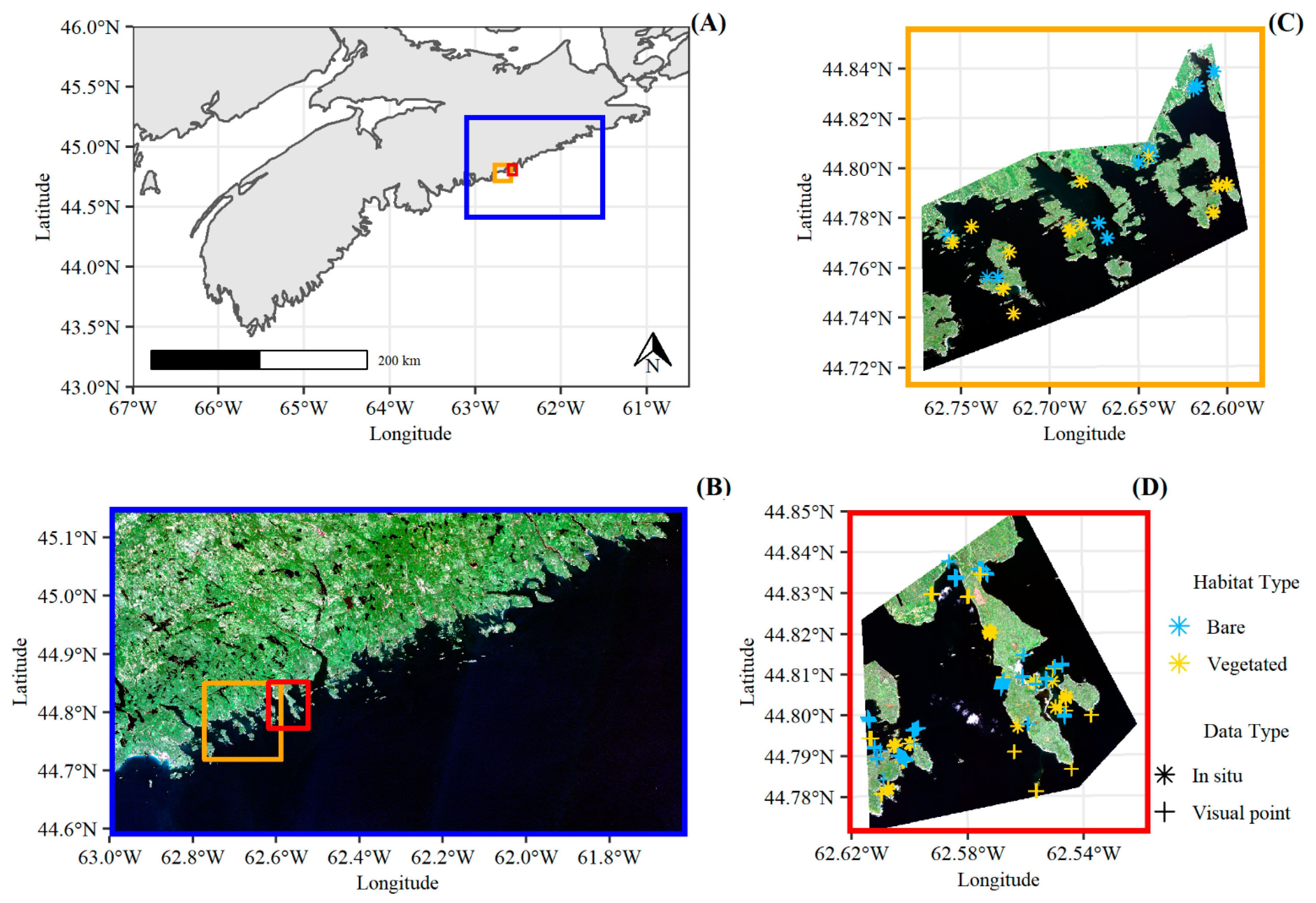
2.1. Study Area and Satellite Data
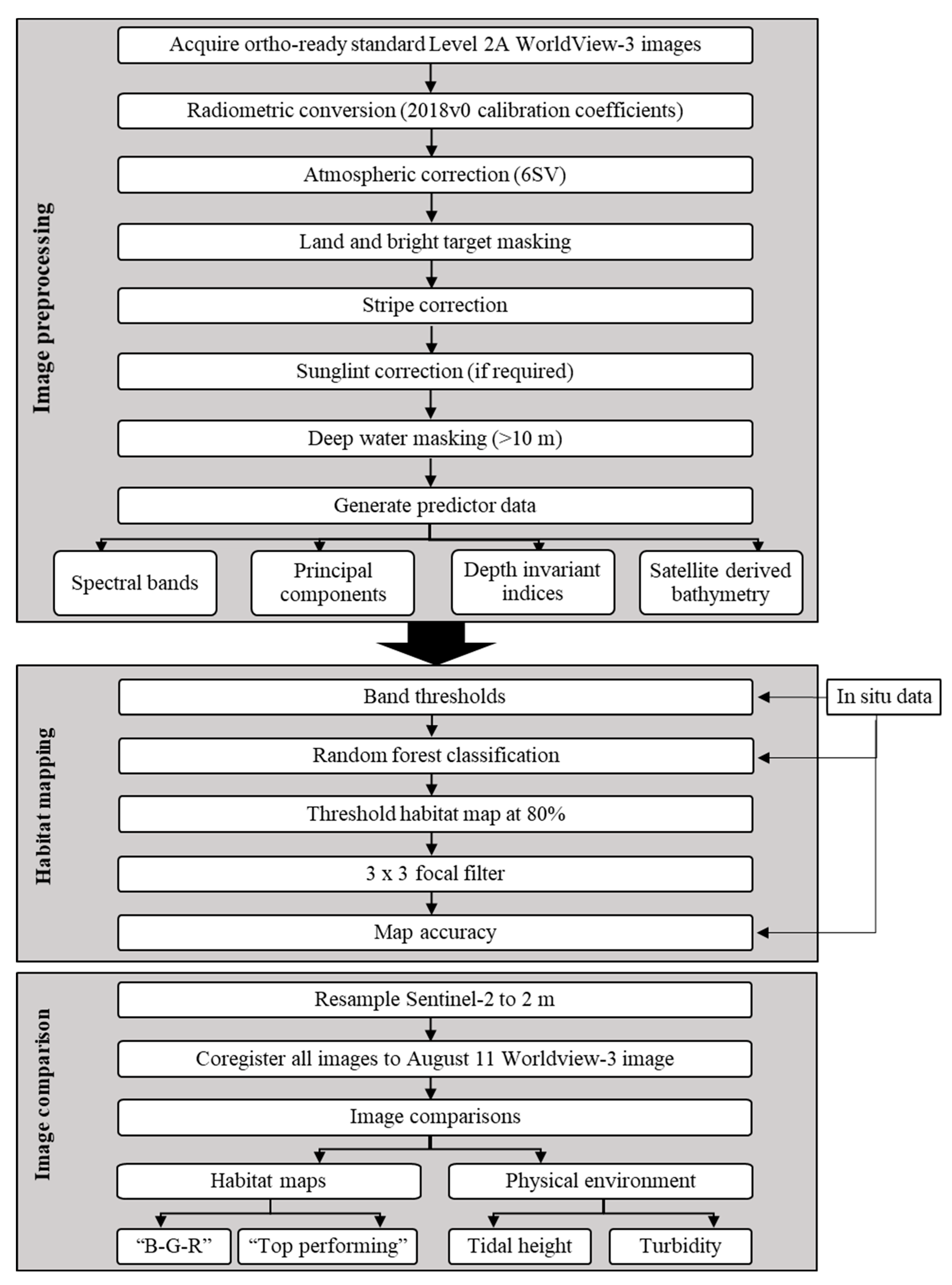
2.2. Image Preprocessing: WorldView-3 Atmospheric and Striping Correction
2.3. Habitat Mapping
2.4. Image Comparison
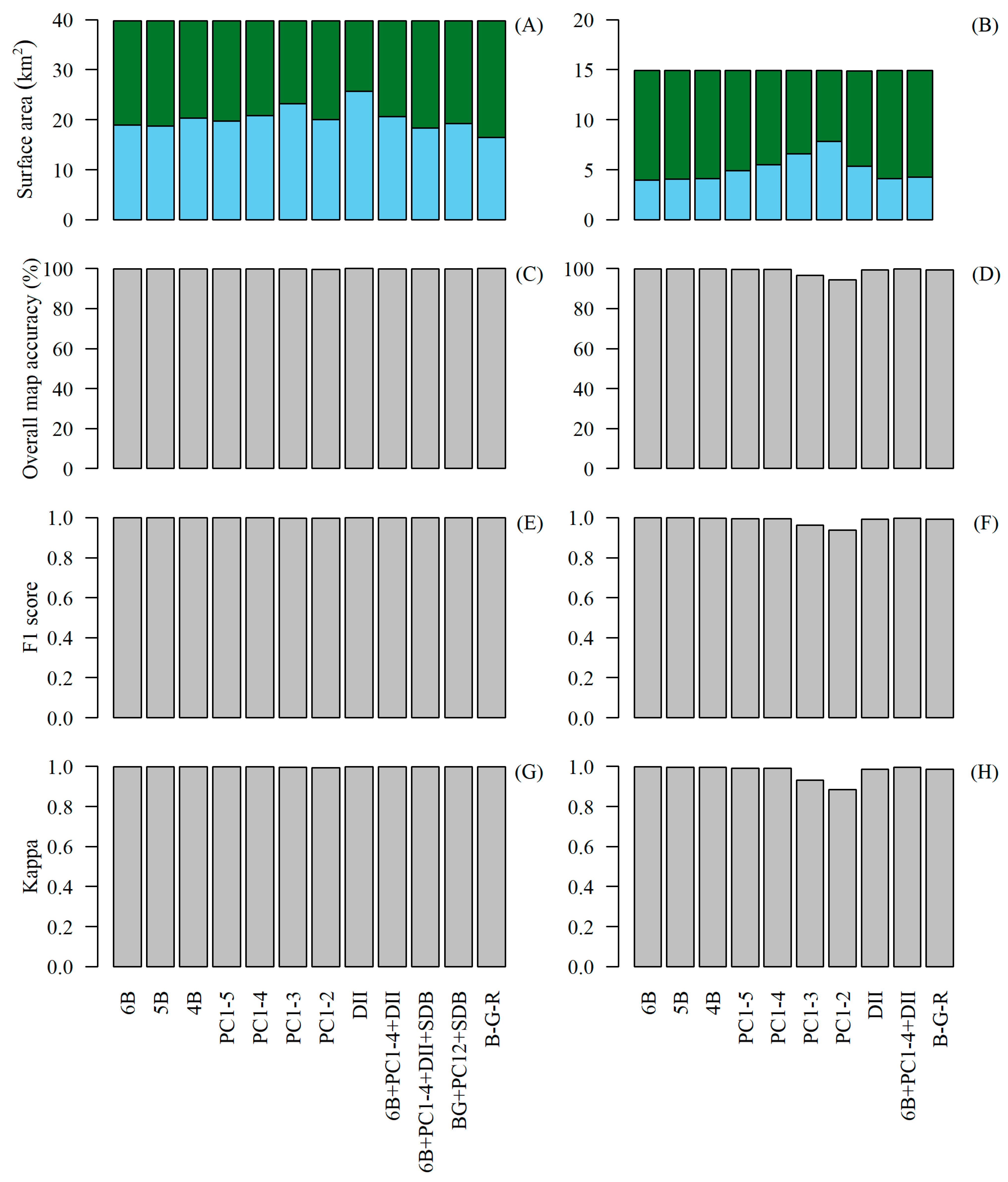
3. Results
4. Discussion
4.1. Generating WorldView-3 Habitat Maps
4.2. Comparing Sentinel-2 and WorldView-3
5. Conclusions
Supplementary Materials
Author Contributions
Funding
Data Availability Statement
Acknowledgments
Conflicts of Interest
Appendix A
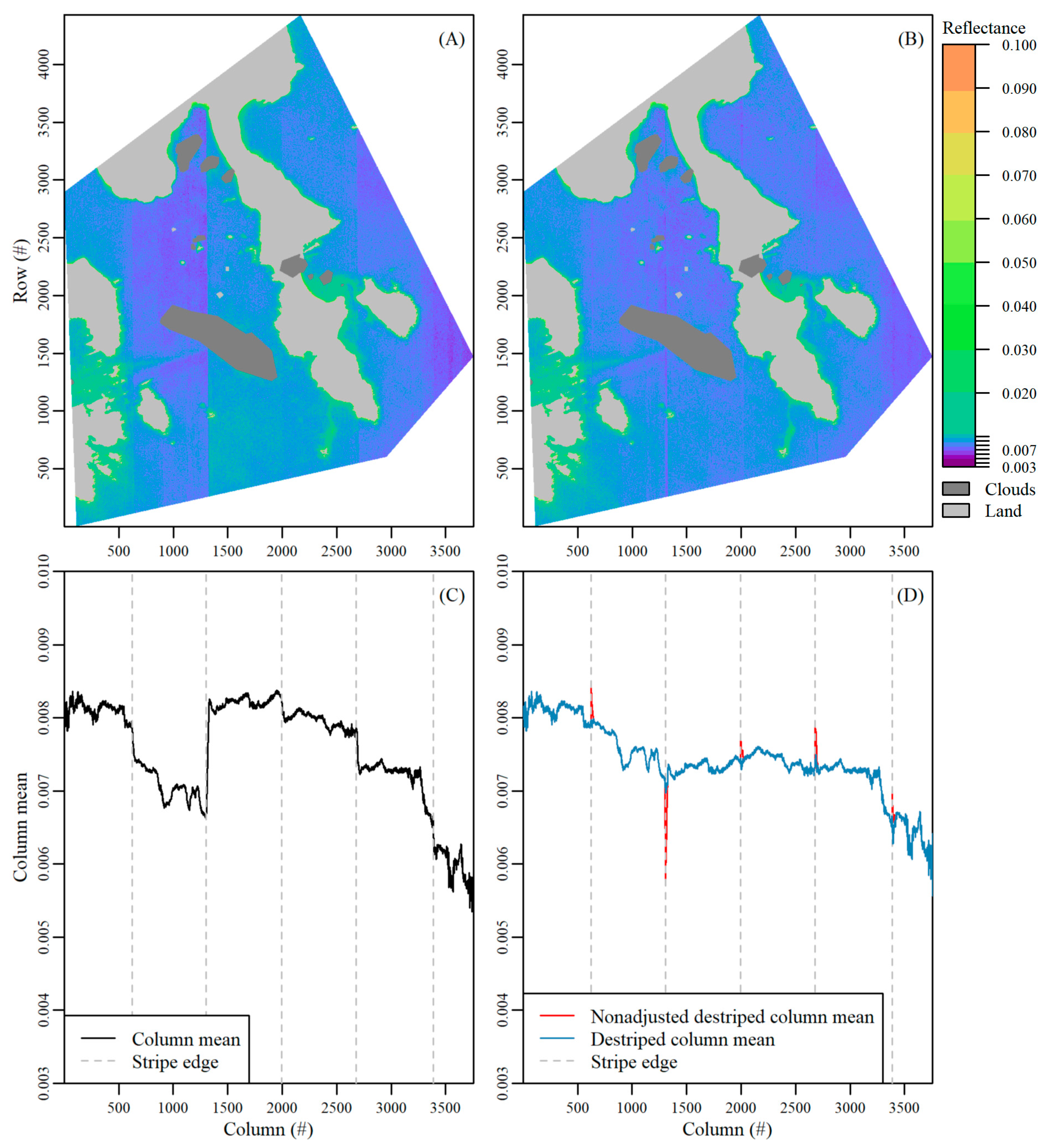
- The mean value per column in the image (column mean) was determined, after masking and excluding bright pixels defined as greater than the 85% quantile of BOA reflectance values over the entire image (Supplementary Material Figure S8a). The bright pixels, which corresponded to nearshore areas where bottom reflection was not negligible, had a large effect on the initial mean column value and created many artificial peaks. Next, columns at the image edges were also masked, as they contained fewer valid rows which resulted in artificial peaks in the column mean values. In this study, we masked the first and last 50 columns for the 11 August image and the first and last 110 columns for the 17 August image. The number of columns was an image-specific number that is dependent on the area of interest, viewing and sun geometry.
- Next, the difference between column mean values following a horizontal (column-wise) lag between columns was calculated (Supplementary Material Figure S8b). An appropriate lag number was image specific. In this study we used lags of 12 and 30 for the 11 August and 17 August images, respectively. The lag was required as stripe edges were not abrupt, but rather spread over a small range of columns, and a stripe may be missed if the difference was calculated only in the adjacent column mean. Next, we found the column index where there were sharp changes in the lagged differences in column means using the findpeaks function in the R package pracma [52]. This column index indicated the edges between various stripes. Sharp changes were defined by setting image specific thresholds for minimum peak height (i.e., minimum difference amount) and distance (i.e., minimum number of consecutive columns). In this study, we set minimum peak height to 0.0002, and 0.0003 for the 11 August and 17 August images, respectively, and peak distance to 500 columns for both images. Note, in Figure S8b, not all spikes above the peak height threshold were identified as a stripe edge as they were closer together than the minimum peak distance allowed. Defining accurate peak height and peak distance thresholds was critical for an accurate stripe edge detection. Lastly, the reference signal to which all other stripes were corrected to was defined by identifying the widest stripe. This arbitrary selection did not impact the habitat classification results as we additionally tested using the first and last stripe as reference with no impact on results.
- Working horizontally outward from the reference signal, an offset value to correct the stripe effect was calculated (Supplementary Material Figure S8c). The importance of the lag in step 2 (see Supplementary Material Figure S8b) was highlighted here. While the stripe edge was identified at column 2675, there was a gradual decline in the column mean value until approximately column 2700 where the column mean became stable. For this same reason, the offset was calculated for a small number of columns away from the stripe edge where the column mean was relatively stable. To do so, the mean of column means for a small subset of columns on opposite sides of the stripe location was calculated. For both images, we took the mean of 10 columns, 40 columns to the left and right from the stripe edge (grey shading in Supplementary Material Figure S8c). The difference between these two means of column means (i.e., difference between reference signal and adjacent signal) were then calculated and added as an offset to all columns within the adjacent stripe. This step was incrementally repeated, working outwards from the reference stripe. Lastly, the masked columns at the scene edges (see Step 1, Supplementary Material Figure S8a) were corrected using the adjacent offset value for the outermost stripes.
- There was over/under correction at stripe edges as stripes gradually transitioned over a small range of image columns. An adjustment was made to the offset value over this range (grey shading Supplementary Material Figure S8d). To do so, we linearly interpolated from the initial to the new offset value for the stripe over the range of columns in which the jump occurs so the offset value was incrementally changed (Supplementary Material Figure S8d). A final vector of offset values was thus created and added to the corresponding image columns to de-stripe the entire image.
- Finally, these steps were applied to each band per image.
References
- Barbier, E.B.; Hacker, S.D.; Kennedy, C.; Koch, E.W.; Stier, A.C.; Silliman, B.R. The value of estuarine and coastal ecosystem services. Ecol. Monogr. 2011, 81, 169–193. [Google Scholar] [CrossRef]
- Wong, M.C.; Kay, L.M. Partial congruence in habitat patterns for taxonomic and functional diversity of fish assemblages in seagrass ecosystems. Mar. Biol. 2019, 166, 46. [Google Scholar] [CrossRef]
- Schmidt, A.L.; Coll, M.; Romanuk, T.N.; Lotze, H.K. Ecosystem structure and services in eelgrass Zostera marina and rockweed Ascophyllum nodosum habitats. Mar. Ecol. Prog. Ser. 2011, 437, 51–68. [Google Scholar] [CrossRef] [Green Version]
- Wong, M.C.; Dowd, M. A model framework to determine the production potential of fish derived from coastal habitats for use in habitat restoration. Estuaries Coasts 2016, 39, 1785–1800. [Google Scholar] [CrossRef]
- Teagle, H.; Hawkins, S.J.; Moore, P.J.; Smale, D.A. The role of kelp species as biogenic habitat formers in coastal marine ecosystems. J. Exp. Mar. Bio. Ecol. 2017, 492, 81–98. [Google Scholar] [CrossRef]
- Duarte, C.M.; Losada, I.J.; Hendriks, I.E.; Mazarrasa, I.; Marba, N. The role of coastal plant communities for climate change mitigation and adaptation. Nat. Clim. Chang. 2013, 3, 961–968. [Google Scholar] [CrossRef] [Green Version]
- Duffy, J.E.; Benedetti-Cecchi, L.; Trinanes, J.; Muller-Karger, F.E.; Ambo-Rappe, R.; Boström, C.; Buschmann, A.H.; Byrnes, J.; Coles, R.G.; Creed, J.; et al. Toward a coordinated global observing system for seagrasses and marine macroalgae. Front. Mar. Sci. 2019, 6, 317. [Google Scholar] [CrossRef] [Green Version]
- Marcello, J.; Eugenio, F.; Gonzalo-Martin, C.; Rodriguez-Esparragon, D.; Marques, F. Advanced processing of multiplatform remote sensing imagery for the monitoring of coastal and mountain ecosystems. IEEE Access 2021, 9, 6536–6549. [Google Scholar] [CrossRef]
- Bennion, M.; Fisher, J.; Yesson, C.; Brodie, J. Remote sensing of kelp (Laminariales, Ochrophyta): Monitoring tools and implications for wild harvesting. Rev. Fish. Sci. Aquac. 2018, 27, 127–141. [Google Scholar] [CrossRef]
- Murphy, G.E.P.; Wong, M.C.; Lotze, H.K. A human impact metric for coastal ecosystems with application to seagrass beds in Atlantic Canada. Facets 2019, 4, 210–237. [Google Scholar] [CrossRef] [Green Version]
- Filbee-Dexter, K.; Wernberg, T. Rise of turfs: A new battlefront for globally declining kelp forests. Bioscience 2018, 68, 64–76. [Google Scholar] [CrossRef] [Green Version]
- Hossain, M.S.; Bujang, J.S.; Zakaria, M.H.; Hashim, M. The application of remote sensing to seagrass ecosystems: An overview and future research prospects. Int. J. Remote Sens. 2015, 36, 61–114. [Google Scholar] [CrossRef]
- Kutser, T.; Hedley, J.; Giardino, C.; Roelfsema, C.M.; Brando, V.E. Remote sensing of shallow waters—A 50 year retrospective and future directions. Remote Sens. Environ. 2020, 240, 111619. [Google Scholar] [CrossRef]
- Rowan, G.S.L.; Kalacska, M. A review of remote sensing of submerged aquatic vegetation for non-specialists. Remote Sens. 2021, 13, 623. [Google Scholar] [CrossRef]
- Vahtmäe, E.; Kutser, T. Classifying the baltic sea shallow water habitats using image-based and spectral library methods. Remote Sens. 2013, 5, 2451–2474. [Google Scholar] [CrossRef] [Green Version]
- Reshitnyk, L.; Costa, M.; Robinson, C.; Dearden, P. Evaluation of WorldView-2 and acoustic remote sensing for mapping benthic habitats in temperate coastal Pacific waters. Remote Sens. Environ. 2014, 153, 7–23. [Google Scholar] [CrossRef]
- Poursanidis, D.; Traganos, D.; Reinartz, P.; Chrysoulakis, N. On the use of Sentinel-2 for coastal habitat mapping and satellite-derived bathymetry estimation using downscaled coastal aerosol band. Int. J. Appl. Earth Obs. Geoinf. 2019, 80, 58–70. [Google Scholar] [CrossRef]
- Mora-Soto, A.; Palacios, M.; Macaya, E.C.; Gómez, I.; Huovinen, P.; Pérez-Matus, A.; Young, M.; Golding, N.; Toro, M.; Yaqub, M.; et al. A high-resolution global map of giant kelp (Macrocystis pyrifera) forests and intertidal green algae (Ulvophyceae) with Sentinel-2 imagery. Remote Sens. 2020, 12, 694. [Google Scholar] [CrossRef] [Green Version]
- Bell, T.W.; Allen, J.G.; Cavanaugh, K.C.; Siegel, D.A. Three decades of variability in California’s giant kelp forests from the Landsat satellites. Remote Sens. Environ. 2020, 238, 110811. [Google Scholar] [CrossRef]
- Topouzelis, K.; Makri, D.; Stoupas, N.; Papakonstantinou, A.; Katsanevakis, S. Seagrass mapping in Greek territorial waters using Landsat-8 satellite images. Int. J. Appl. Earth Obs. Geoinf. 2018, 67, 98–113. [Google Scholar] [CrossRef]
- Poursanidis, D.; Traganos, D.; Teixeira, L.; Shapiro, A.; Muaves, L. Cloud-native seascape mapping of Mozambique’s Quirimbas National Park with Sentinel-2. Remote Sens. Ecol. Conserv. 2021, 7, 275–291. [Google Scholar] [CrossRef]
- Butler, J.D.; Purkis, S.J.; Yousif, R.; Al-Shaikh, I.; Warren, C. A high-resolution remotely sensed benthic habitat map of the Qatari coastal zone. Mar. Pollut. Bull. 2020, 160, 111634. [Google Scholar] [CrossRef] [PubMed]
- Forsey, D.; LaRocque, A.; Leblon, B.; Skinner, M.; Douglas, A. Refinements in eelgrass mapping at Tabusintac Bay (New Brunswick, Canada): A comparison between random forest and the maximum likelihood classifier. Can. J. Remote Sens. 2020, 46, 640–659. [Google Scholar] [CrossRef]
- Wicaksono, P.; Aryaguna, P.A.; Lazuardi, W. Benthic habitat mapping model and cross validation using machine-learning classification algorithms. Remote Sens. 2019, 11, 1279. [Google Scholar] [CrossRef] [Green Version]
- Coffer, M.M.; Schaeffer, B.A.; Zimmerman, R.C.; Hill, V.; Li, J.; Islam, K.A.; Whitman, P.J. Performance across WorldView-2 and RapidEye for reproducible seagrass mapping. Remote Sens. Environ. 2020, 250, 112036. [Google Scholar] [CrossRef]
- Schott, J.R.; Gerace, A.; Woodcock, C.E.; Wang, S.; Zhu, Z.; Wynne, R.H.; Blinn, C.E. The impact of improved signal-to-noise ratios on algorithm performance: Case studies for Landsat class instruments. Remote Sens. Environ. 2016, 185, 37–45. [Google Scholar] [CrossRef] [Green Version]
- Morfitt, R.; Barsi, J.; Levy, R.; Markham, B.; Micijevic, E.; Ong, L.; Scaramuzza, P.; Vanderwerff, K. Landsat-8 Operational Land Imager (OLI) radiometric performance on-orbit. Remote Sens. 2015, 7, 2208–2237. [Google Scholar] [CrossRef] [Green Version]
- Hossain, M.S.; Hashim, M. Potential of Earth Observation (EO) technologies for seagrass ecosystem service assessments. Int. J. Appl. Earth Obs. Geoinf. 2019, 77, 15–29. [Google Scholar] [CrossRef]
- Kovacs, E.; Roelfsema, C.M.; Lyons, M.; Zhao, S.; Phinn, S.R. Seagrass habitat mapping: How do Landsat 8 OLI, Sentinel-2, ZY-3A, and WorldView-3 perform? Remote Sens. Lett. 2018, 9, 686–695. [Google Scholar] [CrossRef]
- Dattola, L.; Rende, F.S.; Di Mento, R.; Dominici, R.; Cappa, P.; Scalise, S.; Aramini, G.; Oranges, T. Comparison of Sentinel-2 and Landsat-8 OLI satellite images vs. high spatial resolution images (MIVIS and WorldView-2) for mapping Posidonia oceanica meadows. Proc. SPIE 2018, 10784, 1078419. [Google Scholar] [CrossRef]
- Wilson, K.L.; Wong, M.C.; Devred, E. Branching algorithm to identify bottom habitat in the optically complex coastal waters of Atlantic Canada using Sentinel-2 satellite imagery. Front. Environ. Sci. 2020, 8, 579856. [Google Scholar] [CrossRef]
- Jeffery, N.W.; Heaslip, S.G.; Stevens, L.A.; Stanley, R.R.E. Biophysical and Ccological Overview of the Eastern Shore Islands Area of Interest (AOI); DFO Canadian Science Advisory Secretariat: Ottawa, ON, Canada, 2020; Volume 2019/025, xiii + 138 p. [Google Scholar]
- Drusch, M.; Del Bello, U.; Carlier, S.; Colin, O.; Fernandez, V.; Gascon, F.; Hoersch, B.; Isola, C.; Laberinti, P.; Martimort, P.; et al. Sentinel-2: ESA’s optical high-resolution mission for GMES operational services. Remote Sens. Environ. 2012, 120, 25–36. [Google Scholar] [CrossRef]
- Marcello, J.; Eugenio, F.; Martín, J.; Marqués, F. Seabed mapping in coastal shallow waters using high resolution multispectral and hyperspectral imagery. Remote Sens. 2018, 10, 1208. [Google Scholar] [CrossRef] [Green Version]
- Kuester, M. Radiometric Use of WorldView-3 Imagery; DigitalGlobe: Longmont, CO, USA, 2016. [Google Scholar]
- DigitalGlobe. WorldView-3 Data Sheet; DigitalGlobe: Longmont, CO, USA, 2014. [Google Scholar]
- MAXAR. Absolute Radiometric Calibration; DigitalGlobe: Longmont, CO, USA, 2018. [Google Scholar]
- Vermote, E.F.; Tanre, D.; Deuze, J.L.; Herman, M.; Morcreyye, J. Second simulation of the satellite signal in the solar spectrum, 6S: An overview. IEEE Trans. Geosci. Remote Sens. 1997, 35. [Google Scholar] [CrossRef] [Green Version]
- Anderson, G.P.; Felde, G.W.; Hoke, M.L.; Ratkowski, A.J.; Cooley, T.W.; Chetwynd, J.H., Jr.; Gardner, J.A.; Adler-Golden, S.M.; Matthew, M.W.; Berk, A.; et al. MODTRAN4-based atmospheric correction algorithm: FLAASH (fast line-of-sight atmospheric analysis of spectral hypercubes). In Algorithms and Technologies for Multispectral, Hyperspectral, and Ultraspectral Imagery VIII; Shen, S.S., Lewis, P.E., Eds.; International Society for Optics and Photonics: Bellingham, WA, USA, 2002; Volume 4725, pp. 65–71. [Google Scholar] [CrossRef]
- Richter, R.; Schläpfer, D. Atmospheric/Topographic Correction for Satellite Imagery: ATCOR-2/3 User Guide; DLR Report; ReSe Applications Schläpfer: Wil, Switzerland, 2015. [Google Scholar]
- Eugenio, F.; Marcello, J.; Martin, J.; Rodríguez-Esparragón, D. Benthic habitat mapping using multispectral high-resolution imagery: Evaluation of shallow water atmospheric correction techniques. Sensors 2017, 17, 2639. [Google Scholar] [CrossRef] [Green Version]
- Vanhellemont, Q. Sensitivity analysis of the dark spectrum fitting atmospheric correction for metre- and decametre-scale satellite imagery using autonomous hyperspectral radiometry. Opt. Express 2020, 28, 29948. [Google Scholar] [CrossRef]
- Vanhellemont, Q.; Ruddick, K. Acolite for Sentinel-2: Aquatic applications of MSI imagery. Eur. Sp. Agency Spec. Publ. ESA SP 2016, SP-740, 9–13. [Google Scholar]
- Marmorino, G.; Chen, W. Use of WorldView-2 along-track stereo imagery to probe a Baltic Sea algal spiral. Remote Sens. 2019, 11, 865. [Google Scholar] [CrossRef] [Green Version]
- R Core Team. R: A Language and Environment for Statistical Computing; R Foundation for Statistical Computing: Vienna, Austria, 2021; Available online: http://www.r-project.org/ (accessed on 18 December 2021).
- de Grandpré, A.; Kinnard, C.; Bertolo, A. Open-Source Analysis of Submerged Aquatic Vegetation Cover in Complex Waters Using High-Resolution Satellite Remote Sensing: An Adaptable Framework. Remote Sens. 2022, 14, 267. [Google Scholar] [CrossRef]
- Lyzenga, D.R. Passive remote sensing techniques for mapping water depth and bottom features. Appl. Opt. 1978, 17, 379. [Google Scholar] [CrossRef]
- Stumpf, R.P.; Holderied, K.; Sinclair, M. Determination of water depth with high-resolution satellite imagery over variable bottom types. Limnol. Oceanogr. 2003, 48, 547–556. [Google Scholar] [CrossRef]
- Hijmans, R.J. Raster: Geographic Data Analysis and Modeling; R Package Version 3.1-5; 2020; Available online: https://rspatial.org/raster/ (accessed on 18 December 2021).
- Benjamin, L.; Horning, N.; Schwalb-willmann, J.; Hijmans, R.J. RStoolbox: Tools for Remote Sensing Data Analysis; R Package Version 0.2.6; 2019; Available online: https://github.com/bleutner/RStoolbox (accessed on 18 December 2021).
- Kuhn, M. Caret: Classification and Regression Training, R Package version 6.0.86; 2020; Available online: https://github.com/topepo/caret/ (accessed on 18 December 2021).
- Borchers, H.W. Pracma: Practical Numerical Math Functions, R Package version 2.3.3; 2021; Available online: https://cran.r-project.org/web/packages/pracma/index.html (accessed on 18 December 2021).
- Wickham, H.; Bryan, J. Readxl: Read Excel Files, R Package version 1.3.1; 2019; Available online: https://github.com/tidyverse/readxl (accessed on 18 December 2021).
- Puspendra, I.F. Irr: Various Coefficients of Interrater Reliability and Agreement, R Package version 0.84.1; 2019; Available online: https://cran.r-project.org/web/packages/irr/index.html (accessed on 18 December 2021).
- Foody, G.M. Status of land cover classification accuracy assessment. Remote Sens. Environ. 2002, 80, 185–201. [Google Scholar] [CrossRef]
- Maxwell, A.E.; Warner, T.A. Thematic classification accuracy assessment with inherently uncertain boundaries: An argument for center-weighted accuracy assessment metrics. Remote Sens. 2020, 12, 1905. [Google Scholar] [CrossRef]
- Ha, N.T.; Manley-Harris, M.; Pham, T.D.; Hawes, I. A comparative assessment of ensemble-based machine learning and maximum likelihood methods for mapping seagrass using Sentinel-2. Remote Sens. 2020, 12, 355. [Google Scholar] [CrossRef] [Green Version]
- Ha, N.T.; Manley-Harris, M.; Pham, T.D.; Hawes, I. The use of radar and optical satellite imagery combined with advanced machine learning and metaheuristic optimization techniques to detect and quantify above ground biomass of intertidal seagrass in a New Zealand estuary. Int. J. Remote Sens. 2021, 42, 4716–4742. [Google Scholar] [CrossRef]
- Dogliotti, A.I.; Ruddick, K.G.; Nechad, B.; Doxaran, D.; Knaeps, E. A single algorithm to retrieve turbidity from remotely-sensed data in all coastal and estuarine waters. Remote Sens. Environ. 2015, 156, 157–168. [Google Scholar] [CrossRef] [Green Version]
- Vanhellemont, Q. ACOLITE Python User Manual (QV—14 January 2021); Royal Belgian Institute of Natural Sciences: Bruxelles, Belgium, 2021. [Google Scholar]
- Nechad, B.; Ruddick, K.; Neukermans, G. Calibration and validation of a generic multisensor algorithm for mapping of turbidity in coastal waters. In Proceedings of the Remote Sensing of the Ocean, Sea Ice, and Large Water Regions 2009, Berlin, Germany, 31 August–3 September 2009; SPIE: Philadelphia, PA, USA, 2009; Volume 7473, pp. 161–171. [Google Scholar] [CrossRef]
- Nechad, B.; Ruddick, K.G.; Park, Y. Calibration and validation of a generic multisensor algorithm for mapping of total suspended matter in turbid waters. Remote Sens. Environ. 2010, 114, 854–866. [Google Scholar] [CrossRef]
- Roelfsema, C.M.; Lyons, M.; Kovacs, E.M.; Maxwell, P.; Saunders, M.I.; Samper-Villarreal, J.; Phinn, S.R. Multi-temporal mapping of seagrass cover, species and biomass: A semi-automated object based image analysis approach. Remote Sens. Environ. 2014, 150, 172–187. [Google Scholar] [CrossRef]
- Wicaksono, P.; Fauzan, M.A.; Kumara, I.S.W.; Yogyantoro, R.N.; Lazuardi, W.; Zhafarina, Z. Analysis of reflectance spectra of tropical seagrass species and their value for mapping using multispectral satellite images. Int. J. Remote Sens. 2019, 40, 8955–8978. [Google Scholar] [CrossRef]
- Su, L.; Huang, Y. Seagrass resource assessment using WorldView-2 imagery in the Redfish Bay, Texas. J. Mar. Sci. Eng. 2019, 7, 98. [Google Scholar] [CrossRef] [Green Version]
- Bakirman, T.; Gumusay, M.U. Assessment of machine learning methods for seagrass classification in the Mediterranean. Balt. J. Mod. Comput. 2020, 8, 315–326. [Google Scholar] [CrossRef]
- Manessa, M.D.M.; Kanno, A.; Sekine, M.; Ampou, E.E.; Widagti, N.; As-Syakur, A.R. Shallow-water benthic identification using multispectral satellite imagery: Investigation on the effects of improving noise correction method and spectral cover. Remote Sens. 2014, 6, 4454–4472. [Google Scholar] [CrossRef] [Green Version]
- Poursanidis, D.; Topouzelis, K.; Chrysoulakis, N. Mapping coastal marine habitats and delineating the deep limits of the Neptune’s seagrass meadows using very high resolution Earth observation data. Int. J. Remote Sens. 2018, 39, 8670–8687. [Google Scholar] [CrossRef]
- Oguslu, E.; Islam, K.; Perez, D.; Hill, V.J.; Bissett, W.P.; Zimmerman, R.C.; Li, J. Detection of seagrass scars using sparse coding and morphological filter. Remote Sens. Environ. 2018, 213, 92–103. [Google Scholar] [CrossRef]
- Nieto, P.; Mücher, C.A. Classifying Benthic Habitats and Deriving Bathymetry at the Caribbean Netherlands Using Multispectral Imagery. Case Study of St. Eustatius; IMARES Rapp. C143/13; IMARES: Wageningen, The Netherlands, 2013; p. 96. [Google Scholar]
- Manuputty, A.; Gaol, J.L.; Agus, S.B.; Nurjaya, I.W. The utilization of depth invariant index and principle component analysis for mapping seagrass ecosystem of Kotok Island and Karang Bongkok, Indonesia. IOP Conf. Ser. Earth Environ. Sci. 2017, 54, 012083. [Google Scholar] [CrossRef] [Green Version]
- Wicaksono, P. Improving the accuracy of multispectral-based benthic habitats mapping using image rotations: The application of principle component analysis and independent componentanalysis. Eur. J. Remote Sens. 2016, 49, 433–463. [Google Scholar] [CrossRef] [Green Version]
- Sebastiá-Frasquet, M.T.; Aguilar-Maldonado, J.A.; Santamaría-Del-ángel, E.; Estornell, J. Sentinel 2 analysis of turbidity patterns in a coastal lagoon. Remote Sens. 2019, 11, 2926. [Google Scholar] [CrossRef] [Green Version]
- Kuhn, C.; de Matos Valerio, A.; Ward, N.; Loken, L.; Sawakuchi, H.O.; Kampel, M.; Richey, J.; Stadler, P.; Crawford, J.; Striegl, R.; et al. Performance of Landsat-8 and Sentinel-2 surface reflectance products for river remote sensing retrievals of chlorophyll-a and turbidity. Remote Sens. Environ. 2019, 224, 104–118. [Google Scholar] [CrossRef] [Green Version]
- Daily Data Report for August 2019. Halifax Stanfield International Airport Nova Scotia. Available online: https://climate.weather.gc.ca/climate_data/daily_data_e.html?hlyRange=2012-09-10%7C2021-06-27&dlyRange=2012-09-10%7C2021-06-27&mlyRange=%7C&StationID=50620&Prov=NS&urlExtension=_e.html&searchType=stnName&optLimit=yearRange&StartYear=1840&EndYear=2021&selR (accessed on 9 July 2021).



| Sentinel-2 | WorldView-3 | |
|---|---|---|
| Spatial resolution (m) | 10 | 2 |
| Spectral resolution (Central wavelength, range (nm)) | Blue (490, 457–522) Green (560, 542–577) Red (665, 650–680) NIR (842, 784–900) | Coastal Blue (427, 400–450) Blue (482, 450–510) Green (547, 510–580) Yellow (604, 585–625) Red (660, 630–690) Red Edge (722, 705–745) NIR1 (824, 770–895) NIR2 (913, 860–1040) |
| Temporal resolution | 5 days at the equator | As tasked |
| Radiometric resolution | 12 bit | 16 bit |
| Cost | Free | $/km2 |
| Image date | 13 September 2016 | 11 August 2019 * 17 August 2019 † |
| Image acquisition time (ADT) | 12:07 | 12:17 * 12:12 † |
| Nearest tidal time (ADT) § | 12:17 | 12:12 * 10:11 † |
| Nearest tidal height (m) § | 0.58 | 0.60 * 1.80 † |
| Name | Spectral Bands | Principal Components | Depth Invariant Indices | SDB | ||||||||||||||||||
|---|---|---|---|---|---|---|---|---|---|---|---|---|---|---|---|---|---|---|---|---|---|---|
| CB | B | G | Y | R | RE | 1 | 2 | 3 | 4 | 5 | CB.B | CB.G | CB.Y | CB.R | B.G | B.Y | B.R | G.Y | G.R | Y.R | ||
| 6B | ||||||||||||||||||||||
| 5B | ||||||||||||||||||||||
| 4B | ||||||||||||||||||||||
| B-G-R | ||||||||||||||||||||||
| PC1-5 | ||||||||||||||||||||||
| PC1-4 | ||||||||||||||||||||||
| PC1-3 | ||||||||||||||||||||||
| PC1-2 | ||||||||||||||||||||||
| DII | ||||||||||||||||||||||
| BG-PC1-2-SDB | ||||||||||||||||||||||
| 6B-PC1-4-DII-SDB | ||||||||||||||||||||||
| 6B-PC1-4-DI | ||||||||||||||||||||||
| Sensor | Band | Center Wavelength | A | C | References |
|---|---|---|---|---|---|
| Sentinel-2 | Red | 665 | 228.10 | 0.1641 | [60] |
| NIR | 842 | 3078.9 | 0.2112 | ||
| WorldView-3 | Red | 661 | 261.11 | 0.1708 | [61,62] |
| RE | 724 | 678.38 | 0.1937 |
Publisher’s Note: MDPI stays neutral with regard to jurisdictional claims in published maps and institutional affiliations. |
© 2022 by the authors. Licensee MDPI, Basel, Switzerland. This article is an open access article distributed under the terms and conditions of the Creative Commons Attribution (CC BY) license (https://creativecommons.org/licenses/by/4.0/).
Share and Cite
Wilson, K.L.; Wong, M.C.; Devred, E. Comparing Sentinel-2 and WorldView-3 Imagery for Coastal Bottom Habitat Mapping in Atlantic Canada. Remote Sens. 2022, 14, 1254. https://doi.org/10.3390/rs14051254
Wilson KL, Wong MC, Devred E. Comparing Sentinel-2 and WorldView-3 Imagery for Coastal Bottom Habitat Mapping in Atlantic Canada. Remote Sensing. 2022; 14(5):1254. https://doi.org/10.3390/rs14051254
Chicago/Turabian StyleWilson, Kristen L., Melisa C. Wong, and Emmanuel Devred. 2022. "Comparing Sentinel-2 and WorldView-3 Imagery for Coastal Bottom Habitat Mapping in Atlantic Canada" Remote Sensing 14, no. 5: 1254. https://doi.org/10.3390/rs14051254
APA StyleWilson, K. L., Wong, M. C., & Devred, E. (2022). Comparing Sentinel-2 and WorldView-3 Imagery for Coastal Bottom Habitat Mapping in Atlantic Canada. Remote Sensing, 14(5), 1254. https://doi.org/10.3390/rs14051254


