Abstract
Soil moisture (SM) is a crucial component for understanding, modeling, and forecasting terrestrial water cycles and energy budgets. However, estimating field-scale SM based on thermal infrared remote-sensing data is still a challenging task. In this study, an improved Flexible Spatiotemporal DAta Fusion (FSDAF) method based on land-surface Diurnal Temperature Cycle (DTC) model (DFSDAF) was proposed to fuse Moderate Resolution Imaging Spectroradiometer (MODIS) and Advance Spaceborne Thermal Emission and Reflection Radiometer (ASTER) land-surface temperature (LST) data to generate ASTER-like LST during the night. The reconstructed diurnal LST data at a high spatial resolution (90 m) was then utilized to drive a two-source normalized soil thermal inertia model (TNSTI) for the vegetated surfaces to estimate field-scale SM. The results of the proposed methods were validated at different observation depths (2, 4, 10, 20, 40, 60, and 100 cm) over the Zhangye oasis in the middle region of the Heihe River basin in the northwest of China and were compared with the SM estimates from the TNSTI model and other SM products, including AMSR2/AMSR-E, GLDAS-Noah, and ERA5-land. The results showed the following: (1) The DFSDAF method increased the accuracy of LST prediction, with the determination coefficient (R2) increasing from 0.71 to 0.77, and root mean square error (RMSE) decreasing from 2.17 to 1.89 K. (2) the estimated SMs had the best correlation with the observations at the 10 cm depth (with R2 of 0.657; RMSE of 0.069 m3/m3), but the worst correlation with observations at the 40 cm depth (with R2 of 0.262; RMSE of 0.092 m3/m3); meanwhile, the modeled SMs were significantly underestimated above 40 cm (2, 4, 10, and 20 cm) and slightly overestimated below 40 cm (60 and 100 cm); in addition, the field-scale SM series at high spatial resolution (90 m) showed significant spatiotemporal variation. (3) The SM estimates based on the TNSTI for the vegetated surfaces are more capable of characterizing the SM status in the root zone (~80 cm) or even deeper, while the SMs from AMSR2/AMSR-E, GLDAS-Noah, or ERA5-land products are closer to the SM in the surface layer (the depth is less than 5 cm). The TNSTI provided favorable data supports for hydrological model simulations and showed potential advantages for agricultural refinement managements and smart agriculture.
1. Introduction
Soil moisture (SM) plays a critical role in monitoring and forecasting land-surface evapotranspiration, agricultural irrigation management, crop yield prediction, weather and climate change, droughts, and hydrologic processes [1,2,3,4,5]. However, it is hard to acquire accurate SM at high spatial–temporal resolution due to the lack of understanding of SM variation within natural landscapes [6,7,8,9]. In situ SM measurements are considered to provide reliable SM data at different depths on different timescales [8,10,11,12,13,14]. However, the spatial representation of field observations suffers weak due to the strong spatial heterogeneity of SM and spare distribution of sites [15]. Although the emergence of new SM measurement methods, such as the Cosmic-ray Soil Moisture Observing System (COSMOS) [16,17], the fiber optic Distributed Temperature Sensing (DTS) system [18], and the Global Positioning System (GPS) [19], shows promising potentiality, the instruments are expensive, time-consuming, and hard to operate. Therefore, ground-based measurements still need to cover a long way in regional applications [20,21]. Comparatively, remote sensing offers a promising approach for large-area applications, benefiting from its high revisiting time and relatively lower cost. Over the past several decades, a series of microwave SM products at the global scale have been produced, such as the active microwave-based products, including European Remote Sensing Satellites (ERS) [22]; Advanced Land Observation Satellite-Phased Array type L-band Synthetic Aperture Radar (ALOS PALSAR) [23]; Sentinel-1 [24], the passive microwave-based products including Advanced Microwave Scanning Radiometer-Earth Observing System (AMSR-E) [25] and Advanced Microwave Scanning Radiometer 2 (AMSR2) [26,27]; WinSAT [28], Soil Moisture Ocean Salinity (SMOS) [29], a combined product (combination of active and passive products) containing Soil Moisture Active Passive (SMAP) [30], and the European Space Agency Climate Change Initiative (ESA CCI) SM products [31,32]. These products are widely used to monitor SM globally [33,34,35,36,37,38]. However, the spatial resolutions of these microwave SM products are coarse, which limited their use in field-scale hydrological and agricultural applications.
Optical remote sensing has the ability to retrieve surface SM at a high spatial resolution [39]; however, the depth of surface SM retrieved from the multispectral images is very shallow due to the poor spectral penetration. In addition, the uncertainty of optical-based surface SM estimates is relatively large, because of the effects of surface roughness, air vapor, soil texture, canopy, and terrain. High-resolution Synthetic Aperture Radar (SAR) shows advantages in all-weather or all-day capability to monitor SM at a large scale based on the backscattered radar signals [40]. However, SAR gave a performance that was unreliable and questionable at the areas covered by vegetation, especially for the short radar wavelengths of SAR. With the development of thermal infrared remote sensing, the spatial and temporal resolution of thermal infrared data has been significantly improved. Thermal infrared remote sensing has been utilized in SM monitoring based on a Vegetation Index/LST (VI/LST) triangular/trapezoidal feature space, such as Crop Water Stress Index (CWSI) [41], Water Deficit Index (WDI) [42], and Temperature Vegetation Dryness Index (TVDI) [43]. However, these thermal infrared-based indices often require ground observations as supporting information and the calculation of them is generally complicated. Soil thermal inertia (STI), as an important soil inherent property of soil, is the function of thermal conductivity, soil bulk density, and specific heat capacity, and is related to the day–night difference of temperature. STI can be used to determine surface characteristics, such as geological lithology identification and analysis [44,45,46], soil moisture, and soil heat flux estimation [45]. The method proposed by Price [47] made the STI retrievable through remote sensing. A series of simplified approaches were proposed in the following decades [48,49,50,51,52]. A large uncertainty was reported in the estimation of STI when applying these methods to the vegetated surfaces [53,54,55]. To overcome this issue, the two-source normalized soil thermal inertia model (TNSTI) model for the vegetated surfaces was proposed by Zhang [56], which made STI possible to be successfully utilized for SM monitoring over the vegetated areas. However, TNSTI required two LST data at different times as the inputs, which limited the employment of single-phase satellite data, such as Landsat and ASTER. Therefore, it is rare to see the reports on the field-scale SM estimates using the TNSTI method over the vegetated areas.
The objectives of this study are (1) to verify the performance of Flexible Spatiotemporal DAta Fusion (FSDAF) and Diurnal Temperature Cycle (DTC) model in FSDAF (DFSDAF) in producing ASTER-like LSTs during the night at high spatial resolution (90 m), (2) to estimate SM at field scale over the vegetated areas using TNSTI model from the reconstructed LSTs, and (3) to evaluate the accuracy of SM estimates from various aspects. The methodology of the DFSDAF method and the TNSTI model for the vegetated surfaces are presented in Section 2. The study area and the datasets are introduced in Section 3. The results and analysis are shown in Section 4. The discussions of the advantages and limitations in this work are provided in Section 5, and conclusions are given in Section 6.
2. Materials and Methods
2.1. DFSDAF
FSDAF needs one pair of fine-resolution and coarse-resolution images acquired at time, and then fine resolution image at time can be reconstruct based on the coarse-resolution image at time. A similar strategy was also employed in Spatial and Temporal Adaptive Reflectance Fusion Model (STARFM) and Enhanced Spatial and Temporal Adaptive Reflectance Fusion Model (ESTARFM), which introduce additional information of similar pixels to reduce the uncertainties and to get a more robust prediction at . Change information of all similar pixels summed by weight is considered as the final total change of the target pixel. Adding the total change to the value of the fine pixel at can realize the final prediction at [57].
where is the size of neighborhood, is the relative distance, is the weight for the similar pixel, and is the change information, which includes spatial change information and temporal change information in two parts. FSDAF is originally designed for fusing the land-surface reflectance data, so is handled as a simple linear variation over time. However, it is not suitable for LST because LST can change distinctively in one day. According to the DTC model [58], LST during the day and LST during the night can be expressed as follows:
where is the temperature amplitude, is the time at which the temperature reaches the maximum value, is the starting time of the free attenuation, is the latitude of the location, and is the solar declination expressed as a function of the day of the year (DOY). Therefore, the temporal change information of can be redefined as the following:
By replacing in the FSDAF method with , we constructed the DFSDAF method.
2.2. TNSTI for the Vegetated Surfaces
In TNSTI, wet soil is mainly assumed to have three parts: dry soil, the air in the soil, and the water in the soil. The thermal inertia of dry soil only depends on its texture and structure, which usually remain the same if the soil type or soil structure does not change. The thermal inertia of the air in the soil is small enough to be ignored. Therefore, the variation of STI is mainly caused by the variation of the water in the soil (namely SM) [56]. The STI is calculated by using the following equation:
where is the mean net radiation from to , is the LST at , and is the LST at . In the same way, STIS for soil thermal inertia and STIV for vegetate fake thermal inertia can be expressed as follows:
where , , and are the mean net radiation at soil surface and soil surface temperature at and , respectively. , , and are the mean net radiation at canopy surface and canopy-surface temperature at and , respectively. and are the function of solar radiation (), surface albedo (), downward longwave radiation () and upward longwave radiation.
where is the Stefan–Boltzmann constant; , , and are the emissivity of soil, vegetation and atmosphere, respectively. is air temperature; , , and are air humidity, saturated air humidity, and relative air humidity, respectively.
The normalized STIs are the representations of relative SM, soil normalized STI (), and vegetation fake normalized STI () and can be defined as follows:
where and are the for bare soil surface at wilting point and saturated status. and are the for fully vegetated surface at wilting point and saturated status, respectively. , , and can be calculated as follows:
where , , , and are the surface temperature at four extreme points in the VI-LST trapezoid space. , , , , , , , and are derived based on the Pixel Component Arranging and Comparing Algorithm (PCACA) model proposed by Zhang [59].
In practice, the water source for bare soil and soil under vegetation are usually not the same. Therefore, a conversion factor, , is needed to correct and .
where the subscript of represents pixel in feature space. The sum of and weighted by fractional vegetation cover () will be the final normalized STI () in mixed pixel.
where and are the surface reflectance of the red band and near infrared band of ASTER, respectively. and are set as 0.02 and 0.88 according to the quantiles of NDVI, respectively.
If SM at wilting point () and SM at saturated status () are given, the estimation of SM content can be defined as the following equation:
3. Study Area and Datasets
3.1. Study Area and Ground-Based Measurements
Zhangye oasis is located in the middle reach of Heihe River basin in the arid and semiarid regions of the northwest of China (100°10′E–100°32′E, 38°44′N–39°00′N; Figure 1), the terrain is relatively flat at about 1550 m above mean sea level. The climate in this region is characterized by cold and dry, with an average annual air temperature of 7.3 °C and precipitation of 130.4 mm (from 1971 to 2010), diurnal temperature difference can reach 15–20 K or more. Cropland, orchard, sandy and Gobi Desert, urban/villages, grassland, and wetland are the main landscapes over Zhangye oasis (Figure 1).
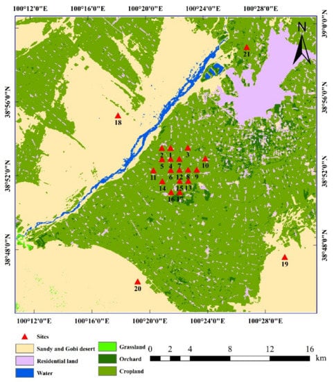
Figure 1.
Distribution of the flux towers and the land-use classifications of Zhangye oasis in the Heihe River basin. The numeric labels are the IDs of the sites.
Heihe Watershed Allied Telemetry Experimental Research (HiWATER) was performed at Heihe River Basin in 2012. An observation matrix composed of 21 stations was constructed in Multi-Scale Observation Experiment on Evapotranspiration (MUSOEXE) over Zhangye oasis [60,61,62]. The distribution of the flux towers is shown in Figure 1. Each station was equipped with a set of Automatic Weather System (AWS), an eddy covariance (EC) system and several soil moisture sensors. AWS acquired meteorological elements, such as air temperature, relative humidity, wind speed, wind direction, air pressure, and net radiation with 10 min intervals. Soil temperature and the soil moisture at different depths (2, 4, 10, 20, 40, 60, and 100 cm) were collected by soil moisture sensors. Table 1 provided detailed information on the instruments equipped at each station for SM observations. Moreover, S3 (short for Site 3), S9, S10, and S16 had only ground-based SM measurements at 2 and 4 cm. Zhangye wetland station (S21) was not equipped with any soil measurement instruments. Daman superstation (S15) was equipped with eight layers of SM observations at depths of 2, 4, 10, 20, 40, 80, 120, and 160 cm, respectively. In addition, four sites (4/20) are placed in bare soil (S4 and S18–S20) and 16 sites (16/20) are placed in the soil under vegetation (S1–S3, S5–S17) (Figure 1). Moreover, each station is also equipped with two vertical downward-pointing Infrared Radiation Thermometers (IRTs) to measure surface temperature. All of these data can be attained from Heihe Plan Science Data Center (http://www.heihedata.org accessed on 1 February 2022) in 2016.

Table 1.
Local overpass time of satellites (UTC + 8 time zone) and the relevant surface observations on the selected 9 days (date format is MM/DD/YYYY); t1 is the overpass time for MODIS Aqua at night, namely the time for the reconstructed ASTER-like data; t2 is the overpass time for ASTER during the day; S0, Ta, and RH are solar radiation, air temperature, and relative air humidity, respectively.
3.2. Remote-Sensing Data and Other SM Products
In this study, nine ASTER images on cloud-free or cloud-few days (15 June-DOY 167, 24 June-DOY 176, 10 July-DOY 192, 2 August-DOY 215, 11 August-DOY 224, 18 August-DOY 231, 27 August-DOY 240, 3 September-DOY 247, and 12 September-DOY 256) in 2012 were acquired from Heihe Plan Science Data Center (http://www.heihedata.org accessed on 1 February 2022) in 2016. The visible and near-infrared (NIR) bands with a spatial resolution of 15 m were used to estimate surface albedo and vegetation fraction. The thermal infrared bands with a spatial resolution of 90 m were adopted to retrieve LST, using a temperature/emissivity separation (TES) approach [63,64]. The local overpass time for ASTER was around 12:10–12:20 p.m. (Table 1). The corresponding MODIS LST products (MOD11A1) were collected from the Land Processes Distributed Active Archive Center (LP DAAC) (http://www.glovis.usgs.gov/ accessed on 1 February 2022). The local overpass time for MODIS Aqua was around 2:10–2:20 a.m. (Table 1). In order to meet the input data requirements of TNSTI model, the LST data of MODIS Aqua during the night were chosen in this study.
The other SM products mainly include the passive microwave SM products from AMSR2/AMSR-E and modeled-based SM products from ERA5-land and GLDAS-Noah. AMSR2/AMSR-E datasets can be freely accessed at https://search.earthdata.nasa.gov accessed on 1 February 2022, ERA5-land SM products can be freely accessed at https://www.ecmwf.int/en/era5-land accessed on 1 February 2022, and GLDAS-Noah SM products can be freely accessed at https://ldas.gsfc.nasa.gov/gldas accessed on 1 February 2022.
4. Results and Analysis
4.1. Validation of Night ASTER-like LSTs from DFSDAF
In order to reduce uncertainty and increase comparability, the average value of two infrared temperature observations at each station was utilized to evaluate the performance of the reconstructed ASTER-like LST during the night. The validation results are shown in Figure 2, and they indicate that the ASTER-like LSTs at night reconstructed by FSDAF and DFSDAF were generally in good agreement with in situ measurements. The determination coefficients (R2) for two methods are all above 0.7, and root mean square errors (RMSEs) are all bellow 2.2 K for these two methods. Compared to FSDAF, the DFSDAF has a higher prediction accuracy, with R2 of 0.771, and RMSE of 1.895 K. Meanwhile, FSDAF performed slightly worse, with R2 of 0.710 and RMSE of 2.173 K. Therefore, the DFSDAF model is more capable of predicting ASTER-like LSTs than FSDAF.
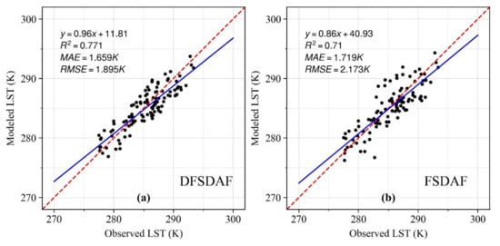
Figure 2.
Validation of night ASTER-like LST by (a) DFSDAF and (b) FSDAF. The red dashed lines are the 1:1 lines, and the blue solid lines represent the best fit linear relationship. R2 is the determination coefficient, MAE is the mean absolute error, and RMSE is the root mean square error.
Statistic comparisons between FSDAF and DFSDAF on the five different land-use types are provided in Table 2. Table 2 shows that the LST during the night was generally cool (<290 K) for all land covers, but there was a slight difference among them. The highest and lowest night LSTs were recorded in wetland and cropland, respectively. Both methods performed better over Gobi/desert or wetland where the surface is relatively more homogeneous than the other land-use types.
Table 2.
Statistic comparisons between FSDAF and DFSDAF on different land-cover types.
The spatial distribution of the ASTER-like LST during the night from DFSDAF and ASTER LST during the day over the Zhangye oasis based on the DFSDAF from DOY 167 to 256 in 2012 is displayed in Figure 3. Generally, the spatial patterns of ASTER-like LST during the night are similar to the patterns of ASTER LST during the day that exhibit significant spatial variability. In addition, the night ASTER-like LSTs are all bellow 300 K, and the diurnal temperature difference can reach 20 K and even more. The higher LST during the night is mainly distributed in water bodies, wetlands, and some urban/villages, due to the slow cooling of water and possible artificial heat sources in urban/villages. Missing values in ASTER-like night LSTs are mainly caused by the missing values in the original MODIS LST products. A small number of clouds affect the reconfiguration result of LST on DOY 224.
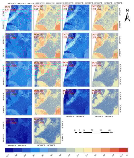
Figure 3.
Spatial distribution of LST during the night (LST_night) from DFSDAF and LST during the day (LST_day) over the Zhangye oasis from DOY 167 to 256 in 2012.
4.2. Validation of SMs from TNSTI for the Vegetated Surfaces
According to the soil hydrological reference data from the West Data Center (http://westdc.westgis.ac.cn/ accessed on 1 February 2022), the SM at wilting point (SMD) and SM at saturated status (SMW) for the Zhangye oasis are 0.072 m3/m3 and 0.356 m3/m3, respectively. The field-scale SMs estimated from the TNSTI model over the vegetated areas were further compared with the in situ SM observations at different depths collected from 20 sites on the selected 9 days. The statistical comparisons are shown in Figure 4.
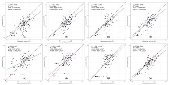
Figure 4.
Comparisons of SM estimates from the TNSTI model over the vegetated areas with in situ observations at different depth: (a) 2 cm, (b) 4cm, (c) 10 cm, (d) 20 cm, (e) 40 cm, (f) 60 cm, and (g) 100 cm; (h) mean of SMs at all depths. The red dashed lines are the 1:1 lines, and the blue solid lines represent the best fit linear relationship. R2 is the determination coefficient, MAE is the mean absolute error, and RMSE is the root mean square error.
The results show an overall reasonably consistent between the estimated SMs and measured SMs at different depths, except for 40 cm in depth (R2 > 0.5). SM estimates correlate with the observations at 10 cm depth at most, with R2 of 0.657 and RMSE of 0.069 m3/m3, while the least correlation is at 40 cm in depth, with R2 of 0.262 and RMSE of 0.092 m3/m3. Moreover, TNSTI has significantly underestimated SMs at 2, 4, 10, and 20 cm depths and slightly overestimated at 60 and 100 cm depths (Figure 4). In addition, by comparing Figure 4h with Figure 4a,b, we see that the correlations between the mean of SMs at all depths and the estimated SMs are superior to those between the SM observations at 2 or 4 cm depth (SM_2 cm or SM_4 cm). It emphasizes that the SMs estimated by TNSTI for the vegetated surfaces are more capable of characterizing the SM variations in the root zone or even deeper, which represents a deeper SM status than that of the microwave SM products (the depth is less than 5 cm). In terms of the depth of estimated SMs, thermal inertia-based SMs estimates outperform the microwave-based SM products.
In order to further investigate the performance of TNSTI in SM estimations based on diurnal LST difference, the comparisons between the estimated SM using TNSTI based on ASTER/ASTER-like LST data (TNSTI_ASTER) and the estimated SM using TNSTI based on MODIS Aqua LST data (TNSTI_MODIS) are also provided in Table 3. Table 3 illustrates that the estimated SMs from TNSTI_MODIS and TNSTI_ASTER are both in good agreement with in situ observations at all depths. However, the TNSTI_ASTER outperforms TNSTI_MODIS at all depths according to the results of the t-test (p < 0.05) with a higher R2 and a lower RMSE. Moreover, the TNSTI_ASTER has a higher spatial resolution (90 m) than TNSTI_MODIS (1 km).
Table 3.
Comparisons between the estimated SM, using TNSTI based on ASTER/ASTER-like LST data, and the estimated SM, using TNSTI based on MODIS Aqua LST data at different depths (2, 4, 10, 20, 40, 60, and 100 cm and the mean SM of all depths).
Moreover, the comparisons between the estimated SMs from TNSTI method for the vegetated surfaces and other SM products, including AMSR2/AMSR-E, GLDAS-Noah, and ERA5-land, were also performed. Observations from all sites were averaged as the final SM representative to match these SM products due to their coarse spatial resolutions. The results (Table 4) show that the estimated SMs from TNSTI model (both SM_TNSTI_MODIS and SM_TNSTI_ASTER) are closer to the SMs in the root zone, while SMs from AMSR2/AMSR-E, GLDAS-Noah, or ERA5-land are closer to SMs in the surface layer. A serious underestimation will occur when using AMSR2/AMSR-E, GLDAS-Noah, or ERA5-land SM products to characterize the root zone SMs in model simulation or hydrological applications.
Table 4.
Comparisons between the estimated SMs from the TNSTI method for the vegetated surfaces and AMSR2/AMSR-E, GLDAS-Noah, and ERA5-land SM products (date format is MM/DD/YYYY; unit is m3/m3 in the table).
Comparisons between SMs estimated by TNSTI and SMs measured at stations on different land-use types are provided in Table 5. It shows that the SM estimated from TNSTI over the vegetated areas is significantly different from the SM at any depth for each land-cover type. This result also reveals that thermal inertia-based SM estimates may reflect the SM status in the root zone or even deeper.
Table 5.
Mean of SM observations at different depths (2, 4, 10, 20, 40, 60, and 100 cm) and mean estimated SM from TNSTI for vegetated surface for each land-use type.
Figure 5 shows the spatial distribution of estimated field-scale SMs from TNSTI for the vegetated surfaces over the Zhangye oasis from DOY 167 to 256 in 2012. The spatial patterns of field-scale SMs based on TNSTI demonstrated significantly spatial variability. The crops over Zhangye oasis are grown from mid-June to early September, and extensive irregular flood irrigations are carried out during this period. Therefore, SM over Zhangye oasis can be maintained at high values. This phenomenon has been well captured by SM estimates from TNSTI at the field scale. SM is relatively low in the early and late crop growth period (DOY 167, 176, 240, 247, and 256), whereas SM is relatively high in the crop growth period (DOY 192, 215, 224, and 231) due to the irrigations. Ignoring the driest sandy and Gobi Desert, the southwest region of Zhangye oasis and Zhangye wetland are slightly wetter than the other regions on DOY 167, 176, 240, and 247. The croplands over Zhanye oasis are overall wet from DOY 192 to 231. SM dries out quickly due to a lack of irrigation from DOY 240. A small number of clouds affected the ASTER-like LST during the night, which led to some unreasonable SM estimates on DOY 224.
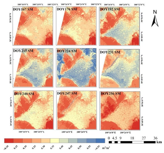
Figure 5.
Spatial distribution of estimated field-scale SMs based on TNSTI for the vegetated surfaces over the Zhangye oasis during the vegetation growing season from June to September in 2012.
Figure 6 presents the time-series behaviors of field-scale SM estimates based on TNSTI for the vegetated surfaces and field observations. The variations of SM from TNSTI over time shows a great consistency with that of the SM measurements. Meanwhile, it showed a big potential advantage in representing the average situation of SM in the root zone or deeper.
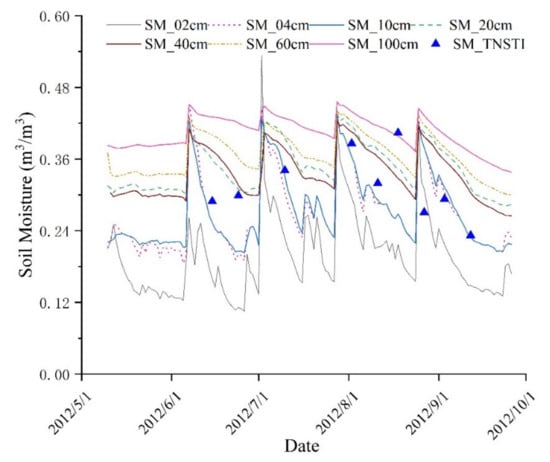
Figure 6.
Time-series comparison between estimated SM based on TNSTI model and in situ observations at different depths. The gray solid line stands for SM at 2 cm, the red dashed line stands for SM at 4 cm, the light blue solid line stands for SM at 10 cm, the light green dashed line stands for SM at 20 cm, the brown solid line stands for SM at 40 cm, the light yellow dashed line stands for SM at 60 cm, the light purple solid line stands for SM at 100 cm, and the triangle deep blue points stands for the SM estimates from TNSTI model.
In summary, the estimated field-scale SMs based on the TNSTI model for the vegetated surfaces over Zhangye oasis are proven reliable and reasonable.
5. Discussion
5.1. Analysis of the Possible Reasons for the Correlations at Different Depths
In order to further explain the possible reasons for the correlations between SM estimates and ground-based observations at different depths, soil-temperature profiles and soil-moisture profiles at the site-scale were analyzed. Figure 7 and Figure 8 show soil-temperature profiles and soil-moisture profiles at Daman superstation (S15) from 8:10 a.m. to 4:10 p.m. on DOY 176, 192, 215, and 247 in 2012, respectively.
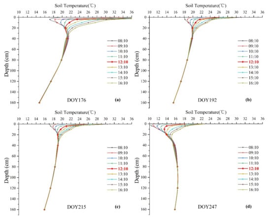
Figure 7.
Soil-temperature profiles at Daman superstation (S15) from 8:10 a.m. to 4:10 p.m. on DOY 176, 192, 215, and 247 in 2012. (a) DOY 176 in June, (b) DOY 192 in July, (c) DOY 215 in August, and (d) DOY 247 in September. The bold red line represents the local overpass time for ASTER.
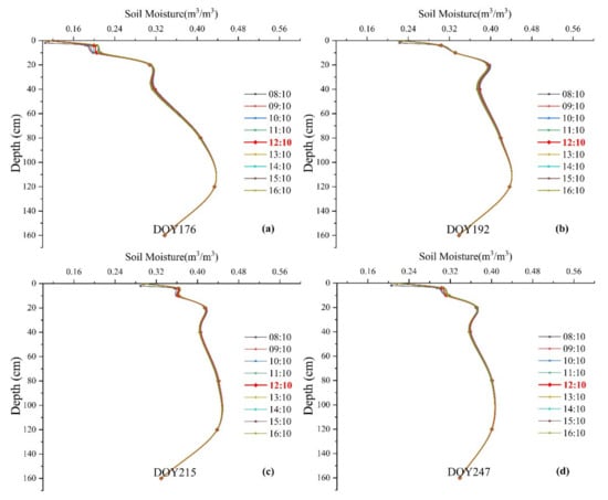
Figure 8.
Soil moisture profiles at Daman superstation (S15) from 8:10 a.m. to 4:10 p.m. on DOY 176, 192, 215, and 247 in 2012. (a) DOY 176 in June, (b) DOY 192 in July, (c) DOY 215 in August, and (d) DOY 247 in September. The red bolded line represents the local overpass time for ASTER.
Figure 7 indicates that the downward solar radiation, which is closely related to soil heat flux, reaches the soil depth of 20 cm from sunrise to overpass time of ASTER. The depth below 20 cm has not been affected by heat energy yet, which is seen from the upward heat flux from 40 cm or deeper. Therefore, the SM estimates based on the TNSTI for the vegetated surface have a higher correlation with the observations above 20 cm. Under the condition that no errors or mistakes happened in the measurements, Figure 8 presents there are two distinct soil inverse wet layers occurring from 0 to 160 cm. One lies in 20 cm to 40 cm, and the other lies from 120 to 160 cm. Soil texture and soil structure may differ significantly above and below the inverse wet layer, which would result in dramatic changes in the soil’s wet and dry conditions as well. This may explain the lowest correlation between estimated SM and the in situ observations at 40 cm depth. Moreover, the existence of SM under the extremely dry status may increase the correlation between SM estimates and the observations at deeper depths (Figure 4f,g).
5.2. Uncertainty and Limitations
The results verify that the TNSTI model can accurately estimate field-scale SM at a spatial resolution of 90 m for the vegetated surfaces. However, some uncertainties and limitations of this method still merit careful attention. (1) TNSTI model is based on Optical/Thermal Infrared (TIR) remote-sensing data, which shows some disadvantages in all-weather or all-day capability compared to the microwave products. (2) TNSTI would be easily affected by clouds, as the accuracy of outputs may decrease for the places with cloud cover. (3) The spatial representation of in situ measurements is limited due to the significant spatial variability of SM, leading to uncertainties in the SMs validations. (4) The quality of the fused LSTs at night may also bring the errors and uncertainties into SMs’ estimates. Moreover, the fused LST at the overpass time of MODIS Aqua is different from the LST at sunrise. Replacing the LST at sunrise with the reconstructed ASTER-like LST at dawn would also produce uncertainties in SM estimates. (5) The determination of the theoretical dry and cold edges in VI-LST trapezoid feature space will also introduce the uncertainty into the normalized STI calculation and the SMs estimates.
Some validations and comparisons of remotely sensed SM estimate models have been conducted over Heihe River Basin. Li [65] used the airborne Polarimetric L-band Multibeam Radiometer (PLMR) and MODIS data to retrieve SM at the spatial resolution of 700 m in the Zhangye oasis and reported that RMSE was 0.04 m3/m3 for SM. Ma [66] applied a real thermal inertia (RTI) model based on MODIS data in Heihe River Basin and showed RMSE of the produced SM was 0.072 m3/m3 and R2 was 0.36, respectively. Luo [67] adopted a change-detection model, constructed using the Sentinel-1 SAR data and MODIS and Landsat 8 Normalized Difference Vegetation Index (NDVI) and showed the Landsat 8 NDVI-based change-detection model slightly outperformed the MODIS NDVI-based model with RMSE of 0.044 m3/m3. Li [68] used the Hydrus-1D model to simulate the soil profile moisture migration process and all the water flux of maize field in the midstream of the Heihe River Basin and showed that RMSE of SM was 0.046 m3/m3. In this study, R2 and RMSE of the modeled SM from TNSTI model are 0.622 and 0.060 m3/m3, respectively. This illustrates that the performance of TNSTI for the SM estimates over the vegetated surfaces is reliable and comparable to the prior studies.
5.3. Future Work
This study provides a feasible method and an operable process for estimating field-scale SM at a high spatial resolution (<100 m) over the vegetated areas. This method is not specifically designed for ASTER data, as it can also be applied to the similar data, such as Landsat-series, HJ-series, GF-series, Sentinel-series, etc., and it can also be performed on other regions or a larger scale. Moreover, new approaches for transforming the LST at dawn into the LST at sunrise and determining the theoretical dry and cold edges in the VI-LST trapezoid feature space are urgently needed to further improve the accuracy of the estimated field-scale SM based on TNSTI model for the vegetated surfaces. In addition, the potential advantages of combining Optical/Thermal Infrared remote sensing and microwave remote sensing in SM estimates should not be ignored. Finally, newly emerging satellite observations at high spatiotemporal resolution for diurnal cycling need to be explored further.
6. Conclusions
In this study, a new method for spatiotemporal data fusion (DFSDAF) was proposed by introducing DTC into FSDAF for characterizing the variations of LST over time. The ASTER-like LSTs during the night were successfully reconstructed by fusing ASTER and MODIS LST, using DFSDAF. The estimation of the field-scale SM at a 90 m spatial resolution based on the TNSTI model for the vegetated surfaces was performed over the Zhangye oasis in the Heihe River basin. The estimated field-scale SMs were compared with in situ observations from the HiWATER-MUSOEXE during the vegetation growing season in 2012.
The results showed that (1) the DFSDAF increases the accuracy of fused LSTs compared to FSDAF (2) TNSTI provides a reliable performance in field-scale SM estimates, which is generally good agreement with the in situ observations. Moreover, the field-scale SM at high spatial resolution (90 m) shows a significant spatiotemporal variability. (3) The estimated SM based on TNSTI for the vegetated surfaces can characterize the SM variations in the root zone or even deeper, which cannot be reflected by the microwave SM products.
In summary, TNSTI effectively improves the capabilities of the field-scale SM estimates over the vegetated surfaces at a high spatial resolution, which can provide favorable data supports for hydrological model simulations and show potential advantages for agricultural refinement management and smart agriculture.
Author Contributions
Conceptualization, G.H. and H.S.; methodology, G.H. and H.S.; software and data processing, G.H.; writing—original draft preparation, G.H.; writing—review and editing, G.H., H.S., J.T., R.Z. and S.C.; visualization, G.H. All authors have read and agreed to the published version of the manuscript.
Funding
This research was funded by National Key Research and Development Program of China (2021YFC3201102) and the National Natural Science Foundation of China grand number (41971315/41571356/U2003105/42071327).
Institutional Review Board Statement
Not applicable.
Informed Consent Statement
Not applicable.
Data Availability Statement
Not applicable.
Acknowledgments
This research was supported by the National Natural Science Foundation of China (Grant No. 41971315/41571356/U2003105/42071327) and National Key Research and Development Program of China (2021YFC3201102). The datasets used in this study are provided by Heihe Plan Science Data Center (http://www.heihedata.org accessed on 1 February 2022). We are very thankful to the staff members in HiWATER-MUSOEXE for their efforts in data collection and sharing, and the National Aeronautics and Space Administration and the United States Geological Survey for providing MODIS data. We would also appreciate the anonymous reviewers for their valuable comments and suggestions for improving this manuscript.
Conflicts of Interest
The authors declare that they have no conflict of interest.
References
- Pasolli, L.; Notarnicola, C.; Bertoldi, G.; Bruzzone, L.; Remelgado, R.; Greifeneder, F.; Niedrist, G.; Della Chiesa, S.; Tappeiner, U.; Zebisch, M. Estimation of Soil Moisture in Mountain Areas Using Svr Technique Applied to Multiscale Active Radar Images at C-Band. IEEE J. Sel. Top. Appl. Earth Obs. Remote Sens. 2015, 8, 262–283. [Google Scholar] [CrossRef]
- Seneviratne, S.I.; Corti, T.; Davin, E.L.; Hirschi, M.; Jaeger, E.B.; Lehner, I.; Orlowsky, B.; Teuling, A.J. Investigating Soil Moisture–Climate Interactions in a Changing Climate: A Review. Earth-Sci. Rev. 2010, 99, 125–161. [Google Scholar] [CrossRef]
- Jin, Y.; Ge, Y.; Wang, J.; Chen, Y.; Heuvelink, G.B.M.; Atkinson, P.M. Downscaling Amsr-2 Soil Moisture Data with Geographically Weighted Area-to-Area Regression Kriging. IEEE Trans. Geosci. Remote Sens. 2018, 56, 2362–2376. [Google Scholar]
- Dirmeyer, P.; Wu, J.; Norton, H.; Dorigo, W.; Quiring, S.; Ford, T.W.; Santanello, J.A.; Bosilovich, M.G.; Ek, M.B.; Koster, R.D.; et al. Confronting Weather and Climate Models with Observational Data from Soil Moisture Networks over the United States. J. Hydrometeorol. 2016, 17, 1049–1067. [Google Scholar] [CrossRef] [PubMed]
- Manning, C.; Widmann, M.; Bevacqua, E.; Van Loon, A.F.; Maraun, D.; Vrac, M. Soil Moisture Drought in Europe: A Compound Event of Precipitation and Potential Evapotranspiration on Multiple Time Scales. J. Hydrometeorol. 2018, 19, 1255–1271. [Google Scholar] [CrossRef]
- Wang, Y.; Peng, J.; Song, X.; Leng, P.; Ludwig, R.; Loew, A. Surface Soil Moisture Retrieval Using Optical/Thermal Infrared Remote Sensing Data. IEEE Trans. Geosci. Remote Sens. 2018, 56, 5433–5442. [Google Scholar] [CrossRef]
- Jian, P.; Shen, H.; He, S.W.; Wu, J.S. Soil Moisture Retrieving Using Hyperspectral Data with the Application of Wavelet Analysis. Environ. Earth Sci. 2012, 69, 279–288. [Google Scholar]
- Vereecken, H.; Huisman, J.A.; Pachepsky, Y.; Montzka, C.; Van Der Kruk, J.; Bogena, H.; Weihermuller, L.; Herbst, M.; Martinez, G.; VanderBorght, J.; et al. On the Spatio-Temporal Dynamics of Soil Moisture at the Field Scale. J. Hydrol. 2014, 516, 76–96. [Google Scholar] [CrossRef]
- Su, Z.; Wen, J.; Dente, L.; van der Velde, R.; Wang, L.; Ma, Y.; Yang, K.; Hu, Z. A Plateau Scale Soil Moisture and Soil Temperature Observatory for Quantifying Uncertainties in Coarse Resolution Satellite Products. Hydrol. Earth Syst. Sci. Discuss. 2011, 8, 243–276. [Google Scholar]
- Dorigo, W.A.; Wagner, W.; Hohensinn, R.; Hahn, S.; Paulik, C.; Xaver, A.; Gruber, A.; Drusch, M.; Mecklenburg, S.; van Oevelen, P.; et al. The International Soil Moisture Network: A Data Hosting Facility for Global in Situ Soil Moisture Measurements. Hydrol. Earth Syst. Sci. 2011, 15, 1675–1698. [Google Scholar] [CrossRef] [Green Version]
- Robock, A.; Vinnikov, K.Y.; Srinivasan, G.; Entin, J.K.; Hollinger, S.E.; Speranskaya, N.A.; Liu, S.; Namkhai, A. The Global Soil Moisture Data Bank. Bull. Am. Meteorol. Soc. 2000, 81, 1281–1300. [Google Scholar] [CrossRef] [Green Version]
- Ahmad, A.B.; Leroux, D.; Kerr, Y.H.; Merlin, O.; Richaume, P.; Sahoo, A.; Wood, E.F. Evaluation of Smos Soil Moisture Products over Continental U.S. Using the Scan/Snotel Network. IEEE Trans. Geosci. Remote Sens. 2012, 50, 1572–1586. [Google Scholar]
- Robinson, D.A.; Campbell, C.S.; Hopmans, J.W.; Hornbuckle, B.K.; Jones, S.B.; Knight, R.; Ogden, F.; Selker, J.; Wendroth, O. Soil Moisture Measurement for Ecological and Hydrological Watershed-Scale Observatories: A Review. Vadose Zone J. 2008, 7, 358–389. [Google Scholar] [CrossRef] [Green Version]
- Niclos, R.; Rivas, R.E.; Garcia-Santos, V.; Dona, C.; Valor, E.; Holzman, M.; Bayala, M.; Carmona, F.; Ocampo, D.; Soldano, A.; et al. SMOS level-2 soil moisture product evaluation in rain-fed croplands of the Pampean region of Argentina. IEEE Trans. Geosci. Remote Sens. 2015, 54, 499–512. [Google Scholar] [CrossRef]
- Li, C.; Lu, H.; Yang, K.; Han, M.; Wright, J.S.; Chen, Y.; Yu, L.; Xu, S.; Huang, X.; Gong, W. The Evaluation of Smap Enhanced Soil Moisture Products Using High-Resolution Model Simulations and in-Situ Observations on the Tibetan Plateau. Remote Sens. 2018, 10, 535. [Google Scholar] [CrossRef] [Green Version]
- Zreda, M.; Desilets, D.; Ferré, T.P.A.; Scott, R.L. Measuring Soil Moisture Content Non-Invasively at Intermediate Spatial Scale Using Cosmic-Ray Neutrons. Geophys. Res. Lett. 2018, 35, L21402. [Google Scholar] [CrossRef] [Green Version]
- Zreda, M.; Shuttleworth, W.J.; Zeng, X.; Zweck, C.; Desilets, D.; Franz, T.; Rosolem, R. Cosmos: The Cosmic-Ray Soil Moisture Observing System. Hydrol. Earth Syst. Sci. 2012, 16, 4079–4099. [Google Scholar] [CrossRef] [Green Version]
- Sayde, C.; Gregory, C.; Gil-Rodriguez, M.; Tufillaro, N.; Tyler, S.; van de Giesen, N.; English, M.; Cuenca, R.; Selker, J. Feasibility of Soil Moisture Monitoring with Heated Fiber Optics. Water Resour. Res. 2010, 46, W06201. [Google Scholar] [CrossRef] [Green Version]
- Larson, K.M.; Small, E.E.; Gutmann, E.D.; Bilich, A.L.; Braun, J.J.; Zavorotny, V.U. Use of Gps Receivers as a Soil Moisture Network for Water Cycle Studies. Geophys. Res. Lett. 2008, 35, L24405. [Google Scholar] [CrossRef] [Green Version]
- Crow, W.T.; Berg, A.A.; Cosh, M.H.; Loew, A.; Mohanty, B.P.; Panciera, R.; de Rosnay, P.; Ryu, D.; Walker, J.P. Upscaling Sparse Ground-Based Soil Moisture Observations for the Validation of Coarse-Resolution Satellite Soil Moisture Products. Rev. Geophys. 2012, 50, RG2002. [Google Scholar]
- Greifeneder, F.; Notarnicola, C.; Bertoldi, G.; Niedrist, G.; Wagner, W. From Point to Pixel Scale: An Upscaling Approach for in Situ Soil Moisture Measurements. Vadose Zone J. 2016, 15, 1–8. [Google Scholar] [CrossRef]
- Berardino, P.; Fornaro, G.; Lanari, R.; Sansosti, E. A New Algorithm for Surface Deformation Monitoring Based on Small Baseline Differential Sar Interferograms. IEEE Trans. Geosci. Remote Sens. 2002, 40, 2375–2383. [Google Scholar] [CrossRef] [Green Version]
- Rosenqvist, A.; Shimada, M.; Ito, N.; Watanabe, M. Alos Palsar: A Pathfinder Mission for Global-Scale Monitoring of the Environment. IEEE Trans. Geosci. Remote Sens. 2007, 45, 3307–3316. [Google Scholar] [CrossRef]
- Paloscia, S.; Pettinato, S.; Santi, E.; Notarnicola, C.; Pasolli, L.; Reppucci, A. Soil Moisture Mapping Using Sentinel-1 Images: Algorithm and Preliminary Validation. Remote Sens. Environ. 2013, 134, 234–248. [Google Scholar] [CrossRef]
- Njoku, E.G.; Jackson, T.J.; Lakshmi, V.; Chan, T.K.; Nghiem, S.V. Soil Moisture Retrieval from Amsr-E. IEEE Trans. Geosci. Remote Sens. 2003, 41, 215–229. [Google Scholar] [CrossRef]
- Parinussa, R.M.; Holmes, T.R.H.; Wanders, N.; Dorigo, W.; De Jeu, R.A.M. A Preliminary Study toward Consistent Soil Moisture from Amsr2. J. Hydrometeorol. 2015, 16, 932–947. [Google Scholar] [CrossRef]
- Imaoka, K.; Kachi, M.; Kasahara, M.; Ito, N.; Nakagawa, K.; Oki, T. Instrument Performance and Calibration of Amsr-E and Amsr2. Int. Arch. Photogramm. Remote Sens. Spat. Inf. Sci. 2010, 38, 13–18. [Google Scholar]
- Gaiser, P.; Germain, K.S.; Twarog, E.; Poe, G.; Purdy, W.; Richardson, D.; Grossman, W.; Jones, W.L.; Spencer, D.; Golba, G.; et al. The Windsat Spaceborne Polarimetric Microwave Radiometer: Sensor Description and Early Orbit Performance. IEEE Trans. Geosci. Remote Sens. 2004, 42, 2347–2361. [Google Scholar] [CrossRef]
- Kerr, Y.H.; Waldteufel, P.; Wigneron, J.-P.; Delwart, S.; Cabot, F.; Boutin, J.; Escorihuela, M.J.; Font, J.; Reul, N.; Gruhier, C.; et al. The Smos Mission: New Tool for Monitoring Key Elements Ofthe Global Water Cycle. Proc. IEEE 2010, 98, 666–687. [Google Scholar] [CrossRef] [Green Version]
- Entekhabi, D.; Njoku, E.G.; O’Neill, P.E.; Kellogg, K.H.; Crow, W.T.; Edelstein, W.N.; Entin, J.K.; Goodman, S.D.; Jackson, T.J.; Johnson, J.; et al. The Soil Moisture Active Passive (Smap) Mission. Proc. IEEE 2010, 98, 704–716. [Google Scholar] [CrossRef]
- Dorigo, W.; Wagner, W.; Albergel, C.; Albrecht, F.; Balsamo, G.; Brocca, L.; Chung, D.; Ertl, M.; Forkel, M.; Gruber, A.; et al. ESA CCI Soil Moisture for Improved Earth System Understanding: State-of-the Art and Future Directions. Remote Sens. Environ. 2017, 203, 185–215. [Google Scholar] [CrossRef]
- Liu, Y.Y.; Parinussa, R.M.; Dorigo, W.A.; De Jeu, R.A.M.; Wagner, W.; van Dijk, A.I.J.M.; McCabe, M.F.; Evans, J.P. Developing an Improved Soil Moisture Dataset by Blending Passive and Active Microwave Satellite-Based Retrievals. Hydrol. Earth Syst. Sci. 2011, 15, 425–436. [Google Scholar] [CrossRef] [Green Version]
- Feng, X.; Li, J.; Cheng, W.; Fu, B.; Wang, Y.; Lü, Y.; Shao, M. Evaluation of Amsr-E Retrieval by Detecting Soil Moisture Decrease Following Massive Dryland Re-Vegetation in the Loess Plateau, China. Remote Sens. Environ. 2017, 196, 253–264. [Google Scholar] [CrossRef]
- AghaKouchak, A.; Farahmand, A.; Melton, F.S.; Teixeira, J.; Anderson, M.C.; Wardlow, B.D.; Hain, C.R. Remote Sensing of Drought: Progress, Challenges and Opportunities. Rev. Geophys. 2015, 53, 452–480. [Google Scholar] [CrossRef] [Green Version]
- Reichle, R.; Liu, Q.; De Lannoy, G.; Crow, W.; Kimball, J.; Koster, R.; Ardizzone, J. Global Assessment of the Smap Level-4 Soil Moisture Product Using Assimilation Diagnostics; American Meteorological Society: Boston, MA, USA, 2018. [Google Scholar]
- Dorigo, W.A.; Gruber, A.; De Jeu, R.A.M.; Wagner, W.; Stacke, T.; Loew, A.; Albergel, C.; Brocca, L.; Chung, D.; Parinussa, R.M.; et al. Evaluation of the Esa Cci Soil Moisture Product Using Ground-Based Observations. Remote Sens. Environ. 2015, 162, 380–395. [Google Scholar] [CrossRef]
- El Sharif, H.; Wang, J.; Georgakakos, A.P. Georgakakos. Modeling Regional Crop Yield and Irrigation Demand Using Smap Type of Soil Moisture Data. J. Hydrometeorol. 2015, 16, 904–916. [Google Scholar] [CrossRef]
- Zhang, X.; Tang, Q.; Liu, X.; Leng, G.; Li, Z. Soil Moisture Drought Monitoring and Forecasting Using Satellite and Climate Model Data over Southwestern China. J. Hydrometeorol. 2016, 18, 5–23. [Google Scholar] [CrossRef]
- Sadeghi, M.; Babaeian, E.; Tuller, M.; Jones, S.B. The Optical Trapezoid Model: A Novel Approach to Remote Sensing of Soil Moisture Applied to Sentinel-2 and Landsat-8 Observations. Remote Sens. Environ. 2017, 198, 52–68. [Google Scholar] [CrossRef] [Green Version]
- Song, K.; Zhou, X.; Fan, Y. Empirically Adopted Iem for Retrieval of Soil Moisture from Radar Backscattering Coefficients. IEEE Trans. Geosci. Remote Sens. 2009, 47, 1662–1672. [Google Scholar] [CrossRef]
- Idso, S.B.; Jackson, R.D.; Pinter, P.J.; Reginato, R.J.; Hatfield, J.L. Normalizing the Stress-Degree-Day Parameter for Environmental Variability. Agric. Meteorol. 1981, 24, 45–55. [Google Scholar] [CrossRef]
- Moran, M.; Clarke, T.; Inoue, Y.; Vidal, A. Estimating Crop Water Deficit Using the Relation between Surface-Air Temperature and Spectral Vegetation Index. Remote Sens. Environ. 1994, 49, 246–263. [Google Scholar] [CrossRef]
- Sandholt, I.; Rasmussen, K.; Andersen, J. A Simple Interpretation of the Surface Temperature/Vegetation Index Space for Assessment of Surface Moisture Status. Remote Sens. Environ. 2002, 79, 213–224. [Google Scholar] [CrossRef]
- Loche, M.; Scaringi, G.; Blahůt, J.; Melis, M.; Funedda, A.; Da Pelo, S.; Erbì, I.; Deiana, G.; Meloni, M.; Cocco, F. An Infrared Thermography Approach to Evaluate the Strength of a Rock Cliff. Remote Sens. 2021, 13, 1265. [Google Scholar] [CrossRef]
- Scaringi, G.; Loche, M. A Thermo-Hydro-Mechanical Approach to Soil Slope Stability under Climate Change. Geomorphology 2022, 401, 108108. [Google Scholar] [CrossRef]
- Melis, M.T.; Da Pelo, S.; Erbì, I.; Loche, M.; Deiana, G.; Demurtas, V.; Meloni, M.A.; Dessì, F.; Funedda, A.; Scaioni, M.; et al. Thermal Remote Sensing from Uavs: A Review on Methods in Coastal Cliffs Prone to Landslides. Remote. Sens. 2020, 12, 1971. [Google Scholar] [CrossRef]
- Price, J.C. Thermal Inertia Mapping: A New View of the Earth. J. Geophys. Res. Earth Surf. 1977, 82, 2582–2590. [Google Scholar] [CrossRef]
- Verhoef, A. Remote Estimation of Thermal Inertia and Soil Heat Flux for Bare Soil. Agric. For. Meteorol. 2004, 123, 221–236. [Google Scholar] [CrossRef]
- Xue, Y.; Cracknell, A.P. Advanced Thermal Inertia Modeling. Int. J. Remote Sens. 1995, 16, 431–446. [Google Scholar] [CrossRef]
- Utsunomiya, Y. Theoretical Analysis of a Thermal Inertia Model for Soil Moisture Estimation and Its Application to Remote Sensing. J. Jpn. Soc. Photogramm. Remote Sens. 1992, 31, 15–26. [Google Scholar] [CrossRef]
- Zhang, R.; Sun, X.; Zhu, Z.; Hongbo, S.U.; Tang, X. A Remote Sensing Model for Monitoring Soil Evaporation Based on Differential Thermal Inertia and Its Validation. Science in China. Ser. D Earth Sci. 2003, 46, 342–355. [Google Scholar]
- Brunt, D. Notes on Radiation in the Atmosphere. I. Q. J. R. Meteorol. Soc. 2010, 58, 389–420. [Google Scholar] [CrossRef]
- Verstraeten, W.W.; Veroustraete, F.; van der Sande, C.J.; Grootaers, I.; Feyen, J. Soil Moisture Retrieval Using Thermal Inertia, Determined with Visible and Thermal Spaceborne Data, Validated for European Forests. Remote Sens. Environ. 2006, 101, 299–314. [Google Scholar] [CrossRef]
- Murray, T.; Verhoef, A. Moving Towards a More Mechanistic Approach in the Determination of Soil Heat Flux from Remote Measurements. Ii. Diurnal Shape of Soil Heat Flux. Agric. For. Meteorol. 2007, 147, 88–97. [Google Scholar] [CrossRef]
- Doninck, J.V.; Peters, J.; Baets, B.D.; Clercq, E.M.D.; Verhoest, N. The Potential of Multitemporal Aqua and Terra Modis Apparent Thermal Inertia as a Soil Moisture Indicator. Int. J. Appl. Earth Obs. Geoinf. 2011, 13, 934–941. [Google Scholar] [CrossRef]
- Zhang, R.; Tian, J.; Mi, S.; Su, H.; He, H.; Li, Z.; Liu, K. The Effect of Vegetation on the Remotely Sensed Soil Thermal Inertia and a Two-Source Normalized Soil Thermal Inertia Model for Vegetated Surfaces. IEEE J. Sel. Top. Appl. Earth Obs. Remote Sens. 2016, 9, 1725–1735. [Google Scholar] [CrossRef]
- Zhu, X.; Helmer, E.H.; Gao, F.; Liu, D.S.; Chen, J.; Lefsky, M.A. A Flexible Spatiotemporal Method for Fusing Satellite Images with Different Resolutions. Remote Sens. Environ. 2016, 172, 165–177. [Google Scholar] [CrossRef]
- Schädlich, S.; Göttsche, F.M.; Olesen, F.S. Influence of Land Surface Parameters and Atmosphere on Meteosat Brightness Temperatures and Generation of Land Surface Temperature Maps by Temporally and Spatially Interpolating Atmospheric Correction. Remote Sens. Environ. 2001, 75, 39–46. [Google Scholar] [CrossRef]
- Zhang, R.; Tian, J.; Su, H.; Sun, X.; Chen, S.; Xia, J. Two Improvements of an Operational Two-Layer Model for Terrestrial Surface Heat Flux Retrieval. Sensors 2008, 8, 6165–6187. [Google Scholar] [CrossRef]
- Li, X.; Cheng, G.; Liu, S.; Xiao, Q.; Ma, M.; Jin, R.; Che, T.; Liu, Q.; Wang, W.; Qi, Y.; et al. Heihe Watershed Allied Telemetry Experimental Research (Hiwater): Scientific Objectives and Experimental Design. Bull. Am. Meteorol. Soc. 2013, 94, 1145–1160. [Google Scholar] [CrossRef]
- Liu, S.; Xu, Z.; Song, L.; Zhao, Q.; Ge, Y.; Xu, T.; Ma, Y.; Zhu, Z.; Jia, Z.; Zhang, F. Upscaling Evapotranspiration Measurements from Multi-Site to the Satellite Pixel Scale over Heterogeneous Land Surfaces. Agric. For. Meteorol. 2016, 230, 97–113. [Google Scholar] [CrossRef]
- Xu, Z.; Liu, S.; Li, X.; Shi, S.; Wang, J.; Zhu, Z.; Xu, T.; Wang, W.; Ma, M. Intercomparison of Surface Energy Flux Measurement Systems Used During the Hiwater-Musoexe. J. Geophys. Res. Atmos. 2013, 118, 13–140. [Google Scholar] [CrossRef]
- Gillespie, A.; Rokugawa, S.; Matsunaga, T.; Cothern, J.S.; Hook, S.; Kahle, A.B. A temperature and emissivity separation algorithm for advanced spaceborne thermal emission. IEEE Trans. Geosci. Remote Sens. 1998, 36, 1113–1126. [Google Scholar] [CrossRef]
- Li, H.; Sun, D.; Yu, Y.; Wang, H.; Liu, Y.; Liu, Q.; Du, Y.; Wang, H.; Cao, B. Evaluation of the Viirs and Modis Lst Products in an Arid Area of Northwest China. Remote Sens. Environ. 2014, 142, 111–121. [Google Scholar] [CrossRef] [Green Version]
- Li, D.; Rui, J.; Tao, C.; Jeffrey, W.; Ying, G.; Nan, Y.; Shuguo, W. Soil Moisture Retrieval from Airborne PLMR and MODIS Productsinthe ZhangyeOasisof MiddleStream ofHeihe River Basin, China. Adv. Earth Sci. 2014, 29, 295–305. [Google Scholar]
- Ma, C.; Wang, W.; Han, X.; Li, X. Soil Moisture Retrieval in the Heihe River Basin Based on the Real Thermal Inertia Method. IEEE J. Sel. Top. Appl. Earth Obs. Remote Sens. 2013, 6, 1460–1467. [Google Scholar] [CrossRef]
- Luo, J.; Qiu, J.; Zhao, T.; Wang, D. Sentinel-1 Based Soil Moisture Estimation in Middle Reaches of Heihe River Basin. Remote Sens. Technol. Appl. 2020, 35, 23–32. [Google Scholar]
- Li, D.S.; Ji, X.B.; Zhao, L.W. Simulation of Seed Corn Farmland Soil Moisture Migration Regularity in the Midstream of the Heihe River Basin. Arid. Zone Res. 2015, 32, 467–475. [Google Scholar]
Publisher’s Note: MDPI stays neutral with regard to jurisdictional claims in published maps and institutional affiliations. |
© 2022 by the authors. Licensee MDPI, Basel, Switzerland. This article is an open access article distributed under the terms and conditions of the Creative Commons Attribution (CC BY) license (https://creativecommons.org/licenses/by/4.0/).