A Comparison of the Performances of Unmanned-Aerial-Vehicle (UAV) and Terrestrial Laser Scanning for Forest Plot Canopy Cover Estimation in Pinus massoniana Forests

Abstract

Canopy cover is an important indicator and commonly used in forest management applications. Unmanned-Aerial-Vehicle (UAV)—Borne Laser Scanning (ULS) has drawn increasing attention as a new alternative source for forest field inventory due to its spatial resolution comparable to that of Terrestrial Laser Scanning (TLS). In this study, the performance of plot canopy cover estimations from ULS and TLS is investigated. The experiment was conducted in 16 plots from two Pinus massoniana forests with different stand conditions in Guangxi, China. Both the Canopy Height Model (CHM)-based and Individual Tree Delineation (ITD)-based methods were used to estimate the canopy cover. The influence of CHM pixel sizes on the estimations was also analyzed. Our results demonstrated that the accuracies of ULS ($R^2$: 0.992–0.996, $RMSE$: 0.591–0.820%) were better than those of TLS ($R^2$: 0.541–0.846, $RMSE$: 3.642–6.297%) when compared against the reference. The average difference between the ULS and TLS estimations was 6.91%, and the disagreement increased as the forest complexity increased. The reasonable CHM pixel sizes for the canopy cover estimations were 0.07–1.2 m for ULS and 0.07–1.5 m for TLS. This study can provide useful information for the selection of data sources and estimation methods in plot canopy cover mapping.

1. Introduction

Forest canopy cover, which is defined as the proportion of the forest floor covered by the vertical projection of tree crowns [1,2], is directly related to the forest floor microclimate and light conditions [3,4,5] and is commonly used for biophysical and natural resource management applications. The spatially accurate mapping of canopy cover plays a critical role in forest stand structure classification [6], biomass production [7], wildfire behavior simulation [8], and wildlife habitat assessment [9,10].

Traditionally, canopy cover has been obtained from field measurements using sighting tubes [11], line intersect sampling [12], canopy photography [13], and the portable station field-map [14], which are laborious and time consuming. In addition, the field measurements obtained via these methods may be inaccurate because the crown boundaries can be difficult to distinguish in practice, and some subjectivity remains in the field measurement [2]. Compared with field measurements, remote sensing techniques can provide spatially continuous observations with a higher efficiency and at a lower cost. Light detection and ranging (LiDAR) is a promising tool for quantifying forest structural parameters because of its ability to assess 3D information with high precision [15,16,17]. LiDAR has the potential to replace field measurements or even be used to assess the quality of field measurements [5,18,19].

The potential of airborne laser scanning (ALS) from manned aircraft for estimating canopy cover has been investigated since commercial systems have become available. The simplest way to estimate canopy cover from ALS is to calculate the proportion of canopy hits above a specified height threshold [2]. However, this method is slightly biased because the ALS pulses are characterized by oblique observations and are not precisely vertical. Moreover, the sides of crowns are also observed at a certain scan angle, and this bias increases with the scan angle, becoming significant at approximately 40° (20° from the zenith) [13]. To eliminate the effect of oblique pulses on canopy cover estimations, several studies have utilized the rasterized canopy height model (CHM)-based method to estimate the canopy cover from ALS point clouds [2,20,21,22]. In these studies, canopy cover was calculated as the ratio of the number of canopy pixels to the total number of pixels. Allocating the canopy echoes to a grid based on XY coordinates was assumed to reduce this effect.

Several studies have also used mathematical models to estimate canopy cover from ALS. Mathematical models were constructed by investigating the correlations between airborne laser metrics and field-measured canopy cover [19,23,24]. For example, Holmgren et al. [23] utilized proportions of laser returns at certain height intervals derived from ALS data as explanatory variables in simple linear regression models for crown coverage estimation in southern Sweden. They reported a root-mean-square error ($RMSE$) of 4.9% for the tree crown coverage estimation. Melin et al. [24] compared with different remote sensing materials for predicting boreal forest canopy cover and observed a high correlation between the field-measured canopy cover and the selected LiDAR predictor.

The potential of terrestrial laser scanning (TLS) for mapping canopy gaps and structures has also been investigated [25,26,27]. However, compared with ALS canopy cover estimation studies, these studies are relatively fewer. The estimation of vertical canopy cover using TLS has not been studied as intensively. One Study [28] created a raster map of the canopy from TLS, and canopy cover was estimated as the proportion of canopy pixels with $RMSE$ of 8.0–17.9% and bias of 6.8–13.1%.

In recent years, improvements in the convenience and miniaturization of unmanned aerial vehicles (UAVs) have made it a powerful platform for forestry mapping. Combined with LiDAR, UAV laser scanning (ULS) provides higher data acquisition efficiency and flexibility at a lower cost than ALS [29,30] and provides detailed data comparable to that of TLS [31,32,33,34]. By providing a distinct combination of high spatial and temporal resolution, ULS narrows the gap between ALS and TLS systems and provides a new type of high-quality point cloud for forest investigations [33].

Previous studies have examined ULS as an alternative technology to ALS, which digitizes forests in a similar manner with higher altitude [30]. Previous ULS studies have predominantly focused on replicating existing forest attributes from ALS point clouds, such as forest height [35], tree crown diameter [29], stem volume [36], and aboveground biomass [30]. More recently, ULS has gained interest for its potential as an alternative technology to TLS owning to its near-ground perspective and dense point cloud characteristics. The first strict evaluation of ULS on in situ observations was provided by [33] and compared the DBH, tree height, and tree position results with those from TLS in a boreal forest. Similarly, [31] compared the ULS and TLS systems for canopy height and DBH estimation in a forest in the Netherlands, while [32] compared the performance of ULS and TLS with respect to explicit tree modeling and tree volume estimation in a Dutch temperate forest.

There is a growing tendency for foresters to use ULS instead of TLS in forest plot inventories, and this development will dramatically improve the efficiency and reduce costs for plot inventories. Accurate forest plot canopy cover estimations are crucial since mapping the distribution of canopy cover over large areas relies on the plot canopy cover estimations for model calibration and validation. It is necessary to study the performances of ULS and TLS in forest plot canopy cover estimations and how different methods may influence canopy cover estimations.

The main objectives of the present study were, therefore, threefold: (1) to investigate the performances of the recent rapidly developed ULS and the current widely used TLS techniques for plot canopy cover estimation under different forest stand conditions with respect to the manual references; (2) quantify the agreement and disagreement in the canopy cover estimations from ULS and TLS with respect to the CHM-based method and individual tree delineation (ITD)-based method; (3) clarify the influence of the pixel size on canopy cover estimation in the CHM-based method from ULS and TLS. The results from this study can provide practical guidance for the selection of data sources and estimation methods in plot canopy cover mapping.

2. Study Area and Materials

2.1. Study Area

The study was conducted in two coniferous forest sites in southern Guangxi Province, China: Guigang (23°7′N, 109°28′E) and Qinzhou (22°2′N, 108°34′E), as illustrated in Figure 1. The two sites are characterized by a subtropical monsoon climate with an annual rainfall of approximately 1600 mm and an annual average temperature of 21–23 °C. The Guigang site was established in a Pinus massoniana plantation with a very open understory and few evergreen microphanerophytes (Figure 2a). The Pinus massoniana plantation consists predominately of mature forest and had a low tree density of 133 trees/ha. The Qinzhou site was established in a natural forest of Pinus massoniana, which is a young forest with various understory species (Figure 2b). It comprises Pinus massoniana of mixed ages and has a tree density of 311 trees/ha, which is relatively higher than the Guigang site. The Guigang and Qinzhou sites had 11 and 5 plots, respectively, which were scanned by both the ULS and TLS. A total of sixteen plots were used in this study. The Guigang and Qinzhou plots are referred to as the GG plots and QZ plots, respectively, in the following sections.

2.2. LiDAR Data Collection

2.2.1. UAV Laser Scanning Data

The UAV-LiDAR data of the 16 plots were captured on 4 and 5 June 2020, with a Genius UAV LiDAR developed by SureStar, Beijing. The UAV LiDAR area coverage and plot distribution are shown in Figure 2. Each plot at the two sites had a fixed size of 30 m × 30 m. The UAV-LiDAR system consisted of a DJI M200 platform, an R-Fans-16 laser scanner, and an advanced navigation spatial dual-coupled GNSS and IMU sensor. The R-Fans-16 scanner features 16 scan layers with a 30° vertical field of view (FOV). It operates at a wavelength of 905 nm and supports 320,000 points per second. The measurement range of R-Fans-16 is 200 m. The flying height for data acquisition was 40 m above ground level with a speed of 5 m/s, resulting in an average point density of approximately 430 pts/m².

2.2.2. Terrestrial Laser Scanning Data

TLS data acquisition was completed on 28 and 29 May 2020, using the RIEGL VZ-400 laser scanner system. The RIEGL VZ-400 laser scanner system has a 360° field of view in the horizontal direction and 100° in the vertical direction, a maximum range of 600 m, and a measurement rate of 120,000 points per second. At the Guigang site, five scans were performed with an average scanning spacing of 35 m to complete a full coverage of the plots, since the plots in the Guigang site were characterized by clear visibility, little understory vegetation, and sparse tree density. Five scans were performed at the Qingzhou site with an average scanning spacing of 15 m to accommodate the high tree density and abundant understory vegetation in this region. Additional retro-reflective targets were set up during the data collection campaign for the co-registration of scans. The average point density of registered TLS data was 29,471 points per m², with a point spacing of approximately 6 mm.

2.3. Establishment of Reference Data

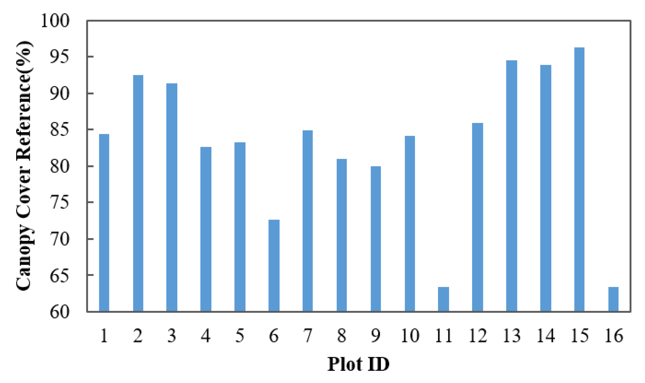
To evaluate the performance of the canopy cover estimation from TLS and ULS, the reference data for the 16 plots were generated by manual measurements from the co-registered TLS and ULS point clouds. The co-registered TLS and ULS point clouds combined the observations from under and above canopy view perspectives with high spatial resolution and were assumed to provide a more reliable canopy cover measurement compared to the use of either TLS or ULS point clouds alone. The ULS point clouds of the plots were manually co-registered to the multi-scan TLS point clouds by selecting common points from the crown boundary and stems. Manual fine-tuning was implemented when a discrepancy between the point clouds remained observable from the top view and two side views. Then, the digital terrain models (DTMs) were created at a 0.2 m resolution from the fused TLS and ULS point clouds using the cloth simulation filter (CSF) method [37]. The fused point cloud height was normalized by subtracting the ground surface height from the DTMs. Finally, the canopy boundaries in each plot were manually delineated from the fused and normalized point clouds, and the canopy cover for each plot was calculated as the ratio of the area of tree crown to the area of the plot. The canopy cover of all 16 plots ranged from 63.37% to 96.28%. Details of the canopy cover distribution are shown in Figure 3.

3. Methods

3.1. Canopy Cover Estimation Using CHM-Based Method

LiDAR-derived CHMs have been widely used to estimate canopy cover [2,21]. To guarantee independence of the canopy cover estimates from different data sources, CHM creations and canopy cover estimations were carried out separately in ULS and TLS point clouds. First, for each sample plot, the ground points and off-ground points were classified from the ULS and TLS point clouds separately, and their DTMs were generated using the CSF method [37] with a 0.2 m × 0.2 m resolution. The TLS and ULS data were normalized with respect to their corresponding DTMs. Then, the normalized point clouds were gridded, and the highest point in each grid was selected to construct the CHMs. To simultaneously describe the tree crown in as much detail as possible and reduce data redundancy, a raw pixel size that was slightly larger than the mean point spacing of the point cloud was used for CHM construction, as reported by [38,39]. In this study, 7 cm and 1 cm were used for the ULS and TLS point clouds, respectively, for CHM construction.

The CHM-based canopy cover was calculated as the percentage of pixels with a CHM value larger than a specified height threshold (canopy pixels):

$$\mathrm{CanopyCover}={{\displaystyle \sum }}^{\text{}}CH{M}_{canopy}/{{\displaystyle \sum }}^{\text{}}CH{M}_{total}$$

(1)

where $CH{M}_{canopy}$ represents the number of canopy pixels (above a specific height threshold) in CHM, and $CH{M}_{total}$ represents the total number of CHM pixels.

Considering the different understory vegetation arrangements in the plots of the two sites (as illustrated in Figure 2), different height thresholds were used to separate the crowns from the background for canopy cover estimation. In the GG plots, since these plots represented clear visibility with sparse understory vegetation, a distance of 2 m was used to separate the crown pixels. In the QZ plots, a distance of 5 m was used to extract crown pixels because of the relatively dense and high shrubs. The within-crown gaps would lead to the underestimation of canopy cover because their CHM values were relatively small (smaller than the height threshold) and were likely to be classified as non-canopy pixels. This situation often occurs in the crown where laser pulses penetrate the gap and reach the ground surface, resulting in a small height value in data collection. Therefore, we utilized the pit-free CHM method proposed by [38] to fill the within-crown gaps of the CHM before canopy cover estimation. This method works by simulating cloth sticking to the CHM surface and filling the within-crown gaps using the hardness of the simulated cloth. The pit-free CHM-based method was capable of filling within-crown gaps while keeping the original CHM pixel values unchanged. The CHM-based canopy cover estimation results from the ULS and TLS data are denoted as ULS_CHM and TLS_CHM, respectively, in the following sections.

We also explored the sensitivity of canopy cover estimation to different CHM pixel sizes for the ULS and TLS point clouds. The original CHMs of ULS and TLS were created under the raw pixel size, which was assumed to describe the crown structure in the most detail. Then, the pixel sizes were increased, from 0.07 to 4.8 m for the ULS and from 0.01 to 2.5 m for the TLS for CHM construction. The canopy cover estimations were then calculated using these CHMs. The canopy cover accuracy was evaluated by comparison with the reference data.

3.2. Canopy Cover Estimation Using ITD-Based Method

To guarantee the independence of the canopy cover estimates from different data sources and to minimize the influences of laser scanning data processing methods, individual tree delineations were manually conducted in the ULS and TLS point clouds separately. Automatic tree detection and modeling methods were not used in this study. Thus, the canopy cover evaluation results revealed the capacities of the applied laser scanning data while excluding the influence of the data processing approach, such as the individual tree detection. Then, each individual tree crown in a plot was accumulated and subtracted from the overlap area to calculate the total crown area. The ITD-based canopy cover was calculated as the percentage of the total crown area to the plot area. The ITD-based canopy cover estimation results from the ULS and TLS data are denoted as ULS_ITD and TLS_ITD, respectively, in the following sections.

3.3. Comparison Scheme and Accuracy Assessment

First, the four canopy cover estimates (ULS_CHM, TLS_CHM, ULS_ITD, and TLS_ITD) were compared with the reference data. Then, the agreement and disagreement in the canopy cover estimations from ULS and TLS were quantified in detail with respect to the CHM-based and ITD-based methods. Finally, the influence of the pixel size on canopy cover estimation in the CHM-based method from ULS and TLS was analyzed.

In this study, the accuracy of the estimated canopy cover was evaluated using the coefficient of determination ($R^2$) and root mean squared error ($RMSE$), which were calculated using the following equations:

$$R^2=1-\frac{{{\displaystyle \sum }}_{i=1}^n{\left(x_i-y_i\right)}^2}{{{\displaystyle \sum }}_{i=1}^n{\left(x_i-\overline{x}\right)}^2}$$

(2)

$$RMSE=\sqrt{\frac{{{\displaystyle \sum }}_{i=1}^n{\left(x_i-y_i\right)}^2}{n}}$$

(3)

where $x_i$ and $y_i$ are the values from the $i$th reference and estimated canopy cover values, $\overline{x}$ is the mean of the reference canopy cover, and $n$ is the number of plots.

4. Results

4.1. Comparison of LiDAR Estimations and Reference

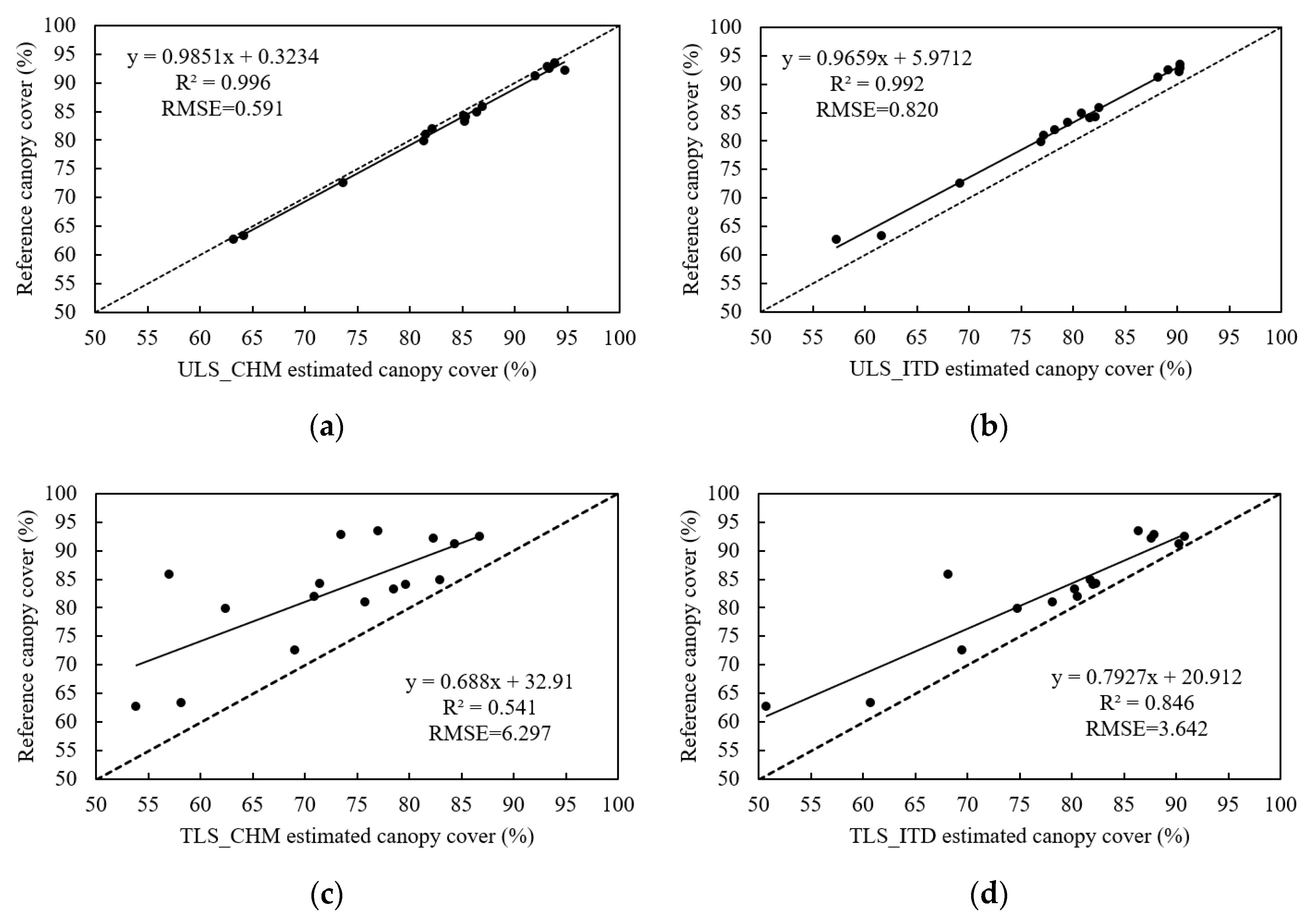
A comparison between the canopy cover estimations from the four methods (i.e., ULS_CHM, ULS_ITD, TLS_CHM, and TLS_ITD) and the reference data are shown in Figure 4 (for all the plots) and Figure 5 (for the GG plots alone). As illustrated in Figure 4, there was an overall moderate to high agreement between the LiDAR-estimated canopy cover and the reference data for all the plots, with $R^2$ values of 0.541–0.996, and $RMSE$ values of 0.591–6.297%. Among the four methods, the ULS_CHM method showed the highest accuracy, with an $R^2$ of 0.996 and an $RMSE$ of 0.591% for canopy cover estimation, while the ULS_ITD method had the second highest accuracy, with an $R^2$ of 0.992 and an $RMSE$ of 0.820%, followed by the TLS_ITD method ($R^2$ = 0.846, $RMSE$ = 3.642%) and the TLS_CHM method ($R^2$ = 0.541, $RMSE$ = 6.297%).

As illustrated in Figure 5, the results from the GG plots alone showed a similar tendency, with the ULS_CHM method showing the highest accuracy ($R^2$ of 0.996, $RMSE$ of 0.476%), followed by the ULS_ITD method ($R^2$ = 0.992, $RMSE$ = 0.685%) and the TLS_ITD method ($R^2$ = 0.986, $RMSE$ = 0.915%). The TLS_CHM method had the lowest accuracy ($R^2$ = 0.737, $RMSE$ = 3.959%). For different forest conditions, the GG plots had a better performance ($R^2$ = 0.737–0.996, $RMSE$ = 0.476–3.959%) than all other plots ($R^2$ = 0.541–0.996, $RMSE$ = 0.591–6.297%).

The overestimation and underestimation of the four methods against the reference data are summarized in

Table 1. Canopy cover differences (%) calculated as ULS/TLS estimations minus reference data for all the plots, the GG plots only, and QZ plots only, where |mean| represents the mean of the absolute values of the difference.

		All Plots			GG Plots			QZ Plots
		Min	Max	|Mean|	Min	Max	|Mean|	Min	Max	|Mean|
ULS	CHM-based	0.07	2.50	0.93	0.07	1.90	0.93	0.33	2.50	0.92
	ITD-based	−5.47	−1.75	3.26	−4.15	−1.75	3.22	−5.47	−2.13	3.34
	Mean			2.10			2.08			2.13
TLS	CHM-based	−28.94	−2.03	10.22	−17.58	−2.03	7.27	−28.94	−8.96	16.73
	ITD-based	−17.75	−1.06	4.69	−5.18	−1.06	2.59	−17.75	−4.70	9.32
	Mean			7.46			4.93			13.03

, which shows the difference between the ULS/TLS estimated canopy cover and the reference data for all the plots, the GG plots only, and the QZ plots only. Overall, the ULS produced smaller deviations than TLS. The mean deviation for the ULS was 2.1% for all the plots and 7.46% for TLS. The ULS_CHM had the smallest deviations, followed by the ULS_ITD, TLS_ITD, and TLS_CHM. In addition, the ULS canopy cover estimations were more robust across different stand conditions and different methods than the TLS estimations. The ULS produced similar deviations between the GG and QZ plots (2.08% vs. 2.13%), whereas significant differences were observed between the corresponding deviations of TLS (4.93% and 13.03%).

4.2. The Agreement and Disagreement in the Estimations from ULS and TLS

A more detailed comparison was conducted directly between the ULS and TLS estimations with respect to different forest conditions and estimation methods. The $R^2$, $RMSE$ and differences between the ULS and TLS estimations were summarized. The disagreement between the ULS and TLS estimations increased with increasing complexity of the forest stand with respect to these metrics.

A moderate agreement was observed between the ULS and TLS estimations when the CHM-based method was used. As illustrated in Figure 6a, the $R^2$ and $RMSE$ between the ULS_CHM and TLS_CHM estimations were 0.554 and 6.288% for all the plots. In the case of the ITD method, the $R^2$ and $RMSE$ between the ULS_ITD and TLS_ITD estimations were $R^2$ 0.859 and 3.600% for all the plots (Figure 6b). For different forest conditions, the GG plots had a higher agreement between the ULS and TLS estimations than all the plots. Figure 6c,d illustrates the comparison on the GG plots, where the ULS and TLS produced an $R^2$ of 0.745 and an $RMSE$ of 3.913% for the CHM-based method, and $R^2$ of 0.985 and an $RMSE$ of 0.919% for the ITD method.

Table 2. Canopy cover differences (%) calculated as ULS estimations minus TLS estimations for all the plots, GG plots only, and QZ plots only, where |mean| represents the mean of the absolute values of the difference.

	All Plots			GG Plots			QZ Plots
	Min	Max	|Mean|	Min	Max	|Mean|	Min	Max	|Mean|
ULS_CHM-TLS_CHM	3.45	29.91	11.15	3.45	18.89	8.19	9.36	29.91	17.65
ULS_ITD-TLS_ITD	−2.33	14.34	2.67	−2.33	2.07	1.17	2.39	14.34	5.97
mean			6.91			4.68			11.81

summarizes the difference between the ULS and TLS estimations for all the plots, the GG plots only, and the QZ plots only. The number of all plots, GG plots, and QZ plots were 16, 11 and 5 respectively. The ULS estimations were larger overall than the TLS estimations for the CHM-based method, with an averaged difference of 11.15% for all the plots. The overestimations in the GG plots were lower than those in the QZ plots. The average overestimation was 8.19% for the GG plots and 17.65% for the QZ plots (Table 2). For the ITD-based method, the TLS estimations tended to be larger in the GG plots and lower in the QZ plots than the ULS estimations (Figure 6b). Only two plots had lower TLS_ITD estimations than the ULS_ITD estimations (Figure 6b). In the QZ plots, the average TLS_ITD estimations were 5.97% lower than ULS_ITD estimations.

4.3. Estimation Results of CHM-Based Canopy Cover with Different Pixel Size

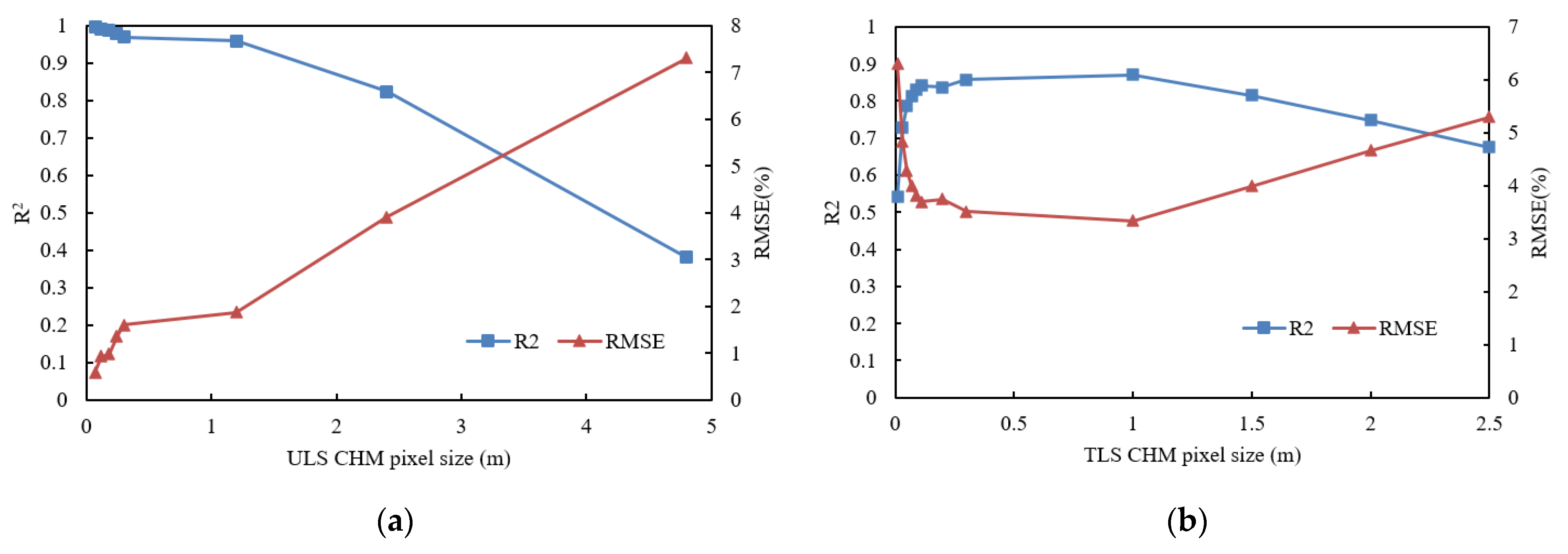
Changes in $R^2$ and $RMSE$ between the CHM-based estimations using different pixel sizes and the reference data are presented in Figure 7. For the ULS_CHM method, the $R^2$ between the ULS_CHM estimations and the reference data decreased with an increase in the pixel size (Figure 7a). The $R^2$ decreased slowly from 0.996 to 0.959 with an increase in the pixel size range from 0.07 m (raw pixel size) to 1.2 m. The decrease rate of $R^2$ was significantly larger after the pixel size exceeded 1.2 m. Conversely, the $RMSE$ values increased as the pixel size increased.

For the TLS_CHM method, $R^2$ initially increased and then decreased with increasing pixel size (Figure 7b). The $R^2$ between the TLS_CHM estimations and reference data increased from 0.541 to 0.871 when the pixel size range increased from 0.01 m (raw pixel size) to 1.0 m. After the pixel size surpassed 1.0 m, $R^2$ rapidly decreased. The $RMSE$ values first decreased and then increased as the pixel size increased.

5. Discussion

5.1. Differences between LiDAR-Derived Canopy Cover and Reference Data

In this study, we compared four LiDAR-estimated canopy covers (ULS_CHM, ULS_ITD, TLS_CHM, and TLS_ITD) with the reference data. The ULS_CHM produced the highest accuracy, followed by ULS_ITD, TLS_ITD, and TLS_CHM. The results demonstrated that the canopy covers obtained using the ULS_CHM method were slightly higher than the reference data, and the canopy covers obtained from the other three methods were lower than the reference data. The higher canopy cover estimations obtained from the ULS_CHM method could be partly attributed to the following aspects: (i) some small between-crown gaps with similar size of within-crown gaps were also filled as canopy pixels, and (ii) the crown boundaries that adjoined the open ground in the horizontal plane tended to expand after the interpolation procedure of the pit-free method.

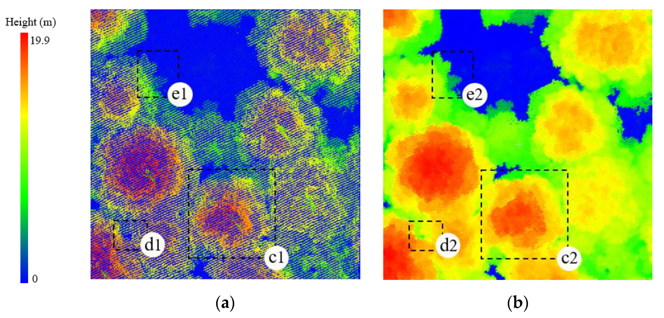
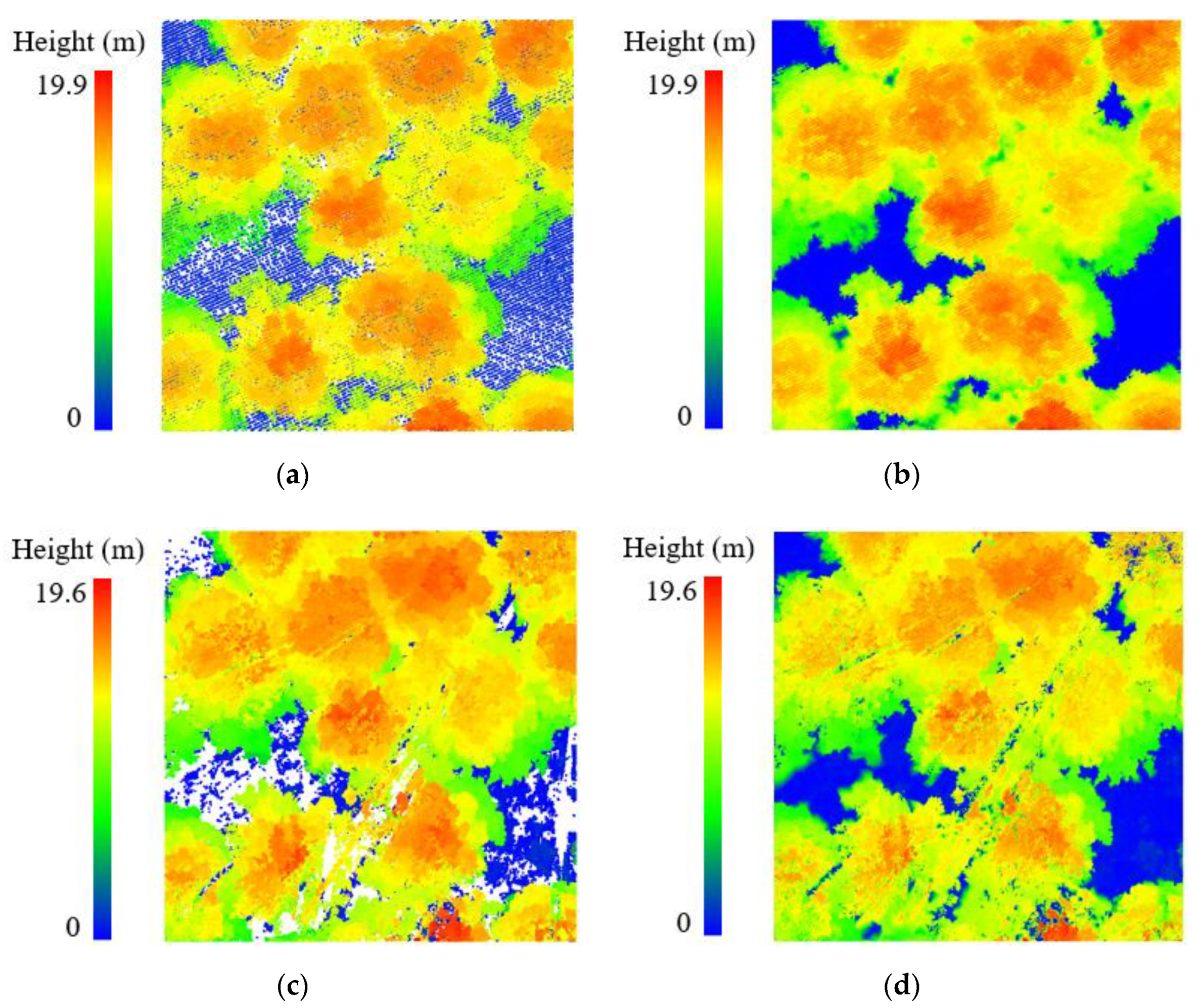
Since the original CHM method would underestimate the canopy cover owing to the existence of within-crown gaps, we utilized the pit-free method proposed by [38] to fill the within-crown gaps to mitigate the underestimation. Our results showed that the pit-free method could effectively remove the within-crown gaps (c1 and c2 in Figure 8a,b). However, the small between-crown gaps with similar within-crown gap size were also interpolated as canopy pixels (d1 and d2 in Figure 8a,b), and the crown boundaries adjacent to the open ground expanded after the pit-free method was applied (e1 and e2 in Figure 8a,b). It was difficult to distinguish between the within-crown gaps and the between-crown gaps with similar sizes and fill the within-crown gaps while ensuring that the between-crown gaps remained unchanged in the CHM smoothing process. The crown boundaries adjacent to the open ground expanded because there were height jumps between the crown boundaries and the adjoining ground. The pit-free method interpolated the pixel values of the adjoining ground and increased their height to reduce the height difference. Thus, several ground pixels were classified as canopy, and the canopy cover was slightly magnified.

In the TLS_CHM method, the canopy cover estimation was lower than the reference, which could be attributed to the incomplete tree crown structure generated from the TLS point clouds. Although the multi-scan mode was used in the TLS data collection, the crowns further away remained occluded when the laser beam was interrupted by stems or branches, and the upper crown of the higher trees was incomplete due to the limited field of view in the vertical direction (−40°–60°). These situations produced within-crown gaps, and these gaps could not be completely removed by the pit-free method, resulting in the underestimation of the TLS_CHM method.

Both the ULS_ITD and TLS_ITD canopy cover estimations were smaller than the reference data, because the reference data were produced from the fused ULS and TLS point clouds. The TLS_ITD canopy cover estimations were lower when the crown boundaries were incomplete in the TLS point clouds. The slightly lower ULS_ITD estimations could be partly attributed to the lower point density of the ULS point clouds when compared with the fused point clouds.

5.2. Difference between ULS-Derived and TLS-Derived Canopy Cover Estimations

In the CHM method, our results demonstrated that the ULS estimations were larger than the TLS estimations for all the plots. The differences between the ULS_CHM and TLS_CHM estimations increased with the increased forest complexity. In the ITD method, the ULS estimations were smaller than the TLS estimations in the simple plots with little understory vegetation and low stem density (GG plots), and the ULS estimations were larger than the TLS estimations in the relatively complex plots with abundant understory growth and higher stem density (QZ plots).

Overall, the ULS tree crowns were more comprehensive than the TLS tree crowns, even when the multi-scan mode was used. Similar results were reported by [28], where ALS produced slight overestimation of canopy cover and TLS underestimated the canopy cover. TLS was vulnerable to the radial occlusion due to the side view perspective and produced gaps within the crowns. These gaps were large and difficult to fill by the CHM smooth method (pit-free), resulting in lower TLS estimations in the CHM-based method. This underestimation grew with increased forest complexity due to the increased occlusion. The QZ plots had denser understory vegetation and higher stem density than the GG plots, resulting in more occlusions in TLS than the GG plots. Therefore, the difference between the ULS_CHM and TLS_CHM estimations for the GG plots (Figure 9) was smaller than that of the QZ plots (Figure 10).

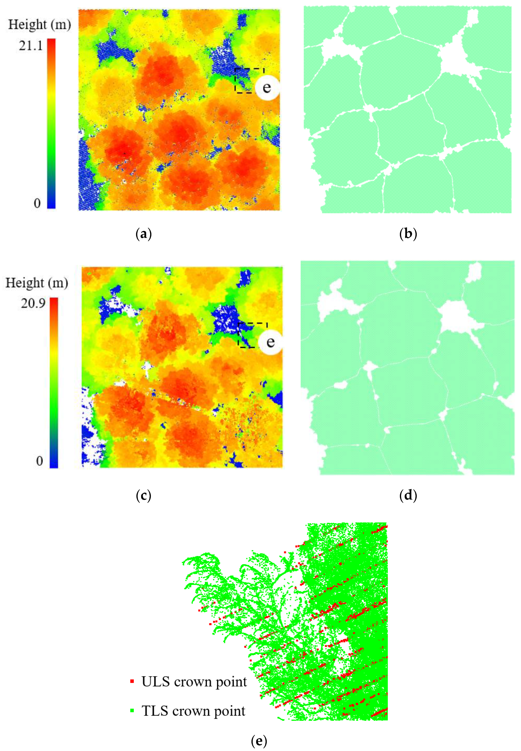
In the ITD method, the TLS estimations were larger than the ULS estimations in simple plots, which can be partly attributed to the denser point density of the TLS point clouds and the fact that the incomplete tree crowns could be recovered as long as crown boundaries existed in the ITD method. The crown boundaries in the simple plots with little understory vegetation and low stem density were more likely to be collected than those in the relatively complex plots with abundant understory growth and higher stem density. Moreover, compared with the ULS crowns, the TLS crowns represented more details and larger areas (as illustrated in Figure 11e). The TLS crown boundaries were more compact, and their between-crown gaps were smaller than those of the ULS (Figure 11b,d). Therefore, the TLS_ITD produced slightly higher estimations than ULS in the simple plots. However, there were two GG plots that produced lower TLS_ITD estimations because their tree crown boundaries were incomplete and the ITD method could not recover the correct crowns areas.

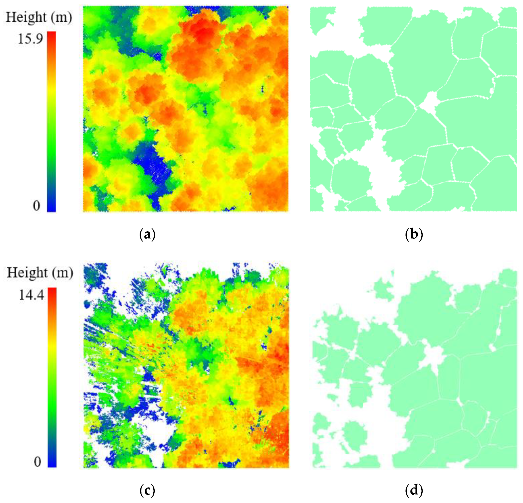
For the QZ plots, the TLS estimations were lower than the ULS estimations in the ITD method. As illustrated in Figure 12b,d, the QZ plots had denser understory vegetation and higher stem density than the GG plots, which led to more severe occlusion and incomplete tree crowns in the TLS point clouds. The crown boundaries were incomplete and the ITD method cannot recover the correct crowns areas, resulting in the underestimation.

5.3. Effect of Pixel Size on the CHM-Based Canopy Cover Estimation Accuracy

The canopy cover estimation increased as the pixel size increased for both the ULS and TLS. This aligned with the results of [38]. When a larger pixel size was used, each within-crown gap was more likely to be assigned to a mixed pixel with crown points, and the gaps were neglected because only the highest point was selected. In addition, the crown boundaries expanded as the pixel size increased, which contributed to an increase in canopy cover values.

For the ULS point clouds, the raw pixel size of the CHM produced slightly overestimated estimations. With increasing pixel size, the overestimation increased when compared with the reference data. Therefore, $R^2$ decreased as the pixel size increased. The $R^2$ decreased slowly and remained relatively constant (0.959–0.996) when the pixel size increased from 0.07 m to 1.2 m, and then decreased significantly again when the pixel size exceeded 1.2 m. The increasing pixel size caused more gaps to be filled as crowns, and the tree crown edges were gradually expanded, resulting in an increase in canopy cover estimation. Reasonable and similar canopy cover estimations could be achieved at pixel sizes ranging from 0.07 m to 1.2 m, which could explain over 95% of the variations in the reference data.

For the TLS point clouds, the raw pixel size of the CHM was underestimated owing to the incomplete tree crown structure. The differences between the CHM estimations and reference data were gradually narrowed at first and then gradually increased with increasing pixel size owing to the increase in canopy cover values. The best agreement was achieved at a pixel size of 1.0 m with an $R^2$ of 0.871 and an $RMSE$ of 3.333%. Reasonable and similar canopy cover estimations could be achieved at a pixel size range of 0.07 m to 1.5 m, which could explain over 80% of the variations in the reference data.

6. Conclusions

Forest canopy cover plays a fundamental role in forest assessment and management. The Sample plot inventories are currently experiencing changes driven by the rapid development of UAV. This study provided a comprehensive cross-comparison of plot canopy cover from the recent rapidly developed ULS and current widely used TLS point clouds over 16 plots in Pinus massoniana forests with different stand conditions in Guangxi, China. Both the CHM- and ITD-based methods were used to estimate the canopy cover for both the ULS and TLS point clouds. Our results illustrated that, compared with the reference data, the ULS_CHM method was the most accurate, with an $R^2$ of 0.996 and $RMSE$ of 0.591%, followed by the ULS_ITD method ($R^2$ = 0.992, $RMSE$ = 0.820%), TLS_ITD method ($R^2$ = 0.846, $RMSE$ = 3.642%), and TLS_CHM method ($R^2$ = 0.541, $RMSE$ = 6.297%). When the ULS estimations were directly compared against the TLS estimations, most ULS estimations were larger than the TLS estimations, with an average difference of 6.91%, and the disagreement increased as the forest complexity increased. The ULS estimations were lower than the TLS estimations; this occurred when the crown boundaries were complete in the ITD method in the simple plots due to the more detailed crowns in the intermediate and suppressed layer than the ULS. In the CHM-based method, the reasonable CHM pixel sizes for the canopy cover estimations were 0.07–1.2 m for ULS and 0.07–1.5 m for TLS. In these ranges, the estimations were marginally influenced by the pixel size. Further work should investigate the estimation performance of canopy cover over large areas from different sources and extend the forest types.

References

1. Jennings, S.B.; Brown, N.D.; Sheil, D. Assessing forest canopies and understorey illumination: Canopy closure, canopy cover and other measures. Forestry 1999, 72, 59–74. [Google Scholar] [CrossRef]
2. Korhonen, L.; Korpela, I.; Heiskanen, J.; Maltamo, M. Airborne discrete-return LIDAR data in the estimation of vertical canopy cover, angular canopy closure and leaf area index. Remote Sens. Environ. 2011, 115, 1065–1080. [Google Scholar] [CrossRef]
3. FAO. On Definitions of Forest and Forest Change. Forest Resources Assessment Programme; Working Paper; FAO: Rome, Italy, 2000; Volume 33, p. 15. [Google Scholar]
4. Gill, S.J.; Biging, G.S.; Murphy, E.C. 2000. Modeling conifer tree crown radius and estimating canopy cover. For. Ecol. Manag. 2000, 126, 405–416. [Google Scholar] [CrossRef] [Green Version]
5. Korhonen, L.; Korhonen, K.T.; Rautiainen, M.; Stenberg, P. Estimation of forest canopy cover: A comparison of field measurement techniques. Silva Fenn. 2006, 40, 577–588. [Google Scholar] [CrossRef] [Green Version]
6. Fiala, A.C.; Garman, S.L.; Gray, A.N. Comparison of five canopy cover estimation techniques in the western Oregon Cascades. For. Ecol. Manag. 2006, 232, 188–197. [Google Scholar] [CrossRef]
7. Chopping, M.; Moisen, G.G.; Su, L.; Lalibrete, A.; Rango, A.; Martonchik, J.; Peter, D.P.C. Large area mapping of southwestern forest crown cover, canopy height, and biomass using the NASA Multiangle Imaging Spectro-Radiometer. Remote Sens. Environ. 2008, 112, 2051–2063. [Google Scholar] [CrossRef] [Green Version]
8. Miller, J.D.; Knapp, E.E.; Key, C.H.; Skinner, C.N.; Isbell, C.J.; Creasy, R.M.; Sherlock, J.W. Calibration and validation of the relative differenced Normalized Burn Ratio (RdNBR) to three measures of fire severity in the Sierra Nevada and Klamath Mountains, California, USA. Remote Sens. Environ. 2009, 113, 645–656. [Google Scholar] [CrossRef]
9. Ganey, J.L.; Cassidy, R.H.; Block, W.M. Estimating Canopy Cover in Forest Stands Used by Mexican Spotted owls: Do Stand-Exam Routines Provide Estimates Comparable to Field-Based Techniques? Res. Pap. RMRS-RP-72WWW; US Department of Agriculture, Forest Service, Rocky Mountain Research Station: Fort Collins, CO, USA, 2008; Volume 8, p. 72.
10. Smart, L.; Swenson, J.; Christensen, N.; Sexton, J. Three-dimensional characterization of pine forest type and red-cockaded woodpecker habitat by small-footprint, discrete-return lidar. For. Ecol. Manag. 2012, 281, 100–110. [Google Scholar] [CrossRef]
11. Rautiainen, M.; Stenberg, P.; Nilson, T. Estimating canopy cover in Scots pine stands. Silva Fenn. 2005, 39, 137–142. [Google Scholar] [CrossRef] [Green Version]
12. Williams, M.S.; Patterson, P.L.; Mowrer, H.T. Comparison of ground sampling methods for estimating canopy cover. For. Sci. 2003, 49, 235–246. [Google Scholar]
13. Korhonen, L.; Heikkinen, J. Automated analysis of in situ canopy images for the estimation of forest canopy cover. For. Sci. 2009, 55, 323–334. [Google Scholar]
14. Santopuoli, G.; di Cristofaro, M.; Kraus, D.; Schuck, A.; Lasserre, B.; Marchetti, M. Biodiversity conservation and wood production in a Natura 2000 Mediterranean forest. A trade-off evaluation focused on the occurrence of microhabitats. IForest 2019, 12, 76. [Google Scholar] [CrossRef] [Green Version]
15. Liang, X.; Wang, Y.; Jaakkola, A.; Kukko, A.; Kaartinen, H.; Hyyppä, J.; Honkavaara, E.; Liu, J. Forest data collection using terrestrial image-based point clouds from a handheld camera compared to terrestrial and personal laser scanning. IEEE Trans. Geosci. Remote Sens. 2015, 53, 5117–5132. [Google Scholar] [CrossRef]
16. Sankey, T.; Donager, J.; McVay, J.; Sankey, J.B. UAV lidar and hyperspectral fusion for forest monitoring in the southwestern USA. Remote Sens. Environ. 2017, 195, 30–43. [Google Scholar] [CrossRef]
17. Schneider, F.D.; Kükenbrink, D.; Schaepman, M.E.; Schimel, D.S.; Morsdorf, F. Quantifying 3D structure and occlusion in dense tropical and temperate forests using close-range LiDAR. Agric. For. Meteorol. 2019, 268, 249–257. [Google Scholar] [CrossRef]
18. Smith, A.M.S.; Falkowski, M.J.; Hudak, A.T.; Evans, J.S.; Robinson, A.P.; Steele, C.M. A cross-comparison of field, spectral and lidar estimates of forest canopy cover. Can. J. Remote Sens. 2009, 35, 447–459. [Google Scholar] [CrossRef]
19. Wu, X.; Shen, X.; Cao, L.; Wang, G.; Cao, F. Assessment of individual tree detection and canopy cover estimation using unmanned aerial vehicle based light detection and ranging (UAV-LiDAR) data in planted forests. Remote Sens. 2019, 11, 908. [Google Scholar] [CrossRef] [Green Version]
20. Lee, A.C.; Lucas, R.M. A LiDAR-derived canopy density model for tree stem and crown mapping in Australian forests. Remote Sens. Environ. 2007, 111, 493–518. [Google Scholar] [CrossRef]
21. Ma, Q.; Su, Y.; Guo, Q. Comparison of canopy cover estimations from airborne LiDAR, aerial imagery, and satellite imagery. IEEE J. Sel. Top. Appl. Earth Obs. Remote Sens. 2017, 10, 4225–4236. [Google Scholar]
22. Liu, Q.; Fu, L.; Wang, G.; Li, S.; Li, Z.; Chen, E.; Pang, Y.; Hu, K. Improving estimation of forest canopy cover by introducing loss ratio of laser pulses using airborne LiDAR. IEEE Trans. Geosci. Remote Sens. 2019, 58, 567–585. [Google Scholar] [CrossRef]
23. Holmgren, J.; Johansson, F.; Olofsson, K.; Olsson, H.; Glimskär, A. Estimation of Crown Coverage Using Airborne Laser Scanning, 8th ed.; SilviLaser 2008 Organizing Committee: Bournemouth, UK, 2008. [Google Scholar]
24. Melin, M.; Korhonen, L.; Kukkonen, M.; Packalen, P. Assessing the performance of aerial image point cloud and spectral metrics in predicting boreal forest canopy cover. ISPRS J. Photogramm. Remote Sens. 2017, 129, 77–85. [Google Scholar] [CrossRef]
25. Danson, F.M.; Hetherington, D.; Morsdorf, F.; Koetz, B.; Allgower, B. Forest canopy gap fraction from terrestrial laser scanning. IEEE Geosci. Remote Sens. Lett. 2007, 4, 157–160. [Google Scholar] [CrossRef] [Green Version]
26. Seidel, D.; Fleck, S.; Leuschner, C. Analyzing forest canopies with ground-based laser scanning: A comparison with hemispherical photography. Agric. For. Meteorol. 2012, 154, 1–8. [Google Scholar] [CrossRef]
27. Cifuentes, R.; Van der Zande, D.; Farifteh, J.; Salas, C.; Coppin, P. Effects of voxel size and sampling setup on the estimation of forest canopy gap fraction from terrestrial laser scanning data. Agric. For. Meteorol. 2014, 194, 230–240. [Google Scholar] [CrossRef]
28. Korhonen, L.; Kaartinen, H.; Kukko, A.; Solberg, S.; Astrup, R. Estimating vertical canopy cover with terrestrial and airborne laser scanning. In Proceedings of the 10th international conference on LiDAR applications for assessing forest ecosystems (Silvilaser 2010), Freiburg, Germany, 14–17 September 2010. [Google Scholar]
29. Li, J.; Yang, B.; Cong, Y.; Cao, L.; Fu, X.; Dong, Z. 3D forest mapping using a low-cost UAV laser scanning system: Investigation and comparison. Remote Sens. 2019, 11, 717. [Google Scholar] [CrossRef] [Green Version]
30. Liu, K.; Shen, X.; Cao, L.; Wang, G.; Cao, F. Estimating forest structural attributes using uav-lidar data in ginkgo plantations. ISPRS J. Photogramm. Remote Sens. 2018, 146, 465–482. [Google Scholar] [CrossRef]
31. Brede, B.; Lau, A.; Bartholomeus, H.M.; Kooistra, L. Comparing RIEGL RiCOPTER UAV LiDAR derived canopy height and DBH with terrestrial LiDAR. Sensors 2017, 17, 2371. [Google Scholar] [CrossRef] [PubMed]
32. Brede, B.; Calders, K.; Lau, A.; Raumonen, P.; Bartholomeus, H.M.; Herold, M.; Kooistra, L. Non-destructive tree volume estimation through quantitative structure modelling: Comparing uav laser scanning with terrestrial lidar. Remote Sens. Environ. 2019, 233, 111355. [Google Scholar] [CrossRef]
33. Liang, X.; Wang, Y.; Pyörälä, J.; Lehtomäki, M.; Yu, X.; Kaartinen, H.; Kukko, E.H.; Issaoui, A.E.I.; Nevalainen, O.; Vaaja, M.; et al. Forest in situ observations using unmanned aerial vehicle as an alternative of terrestrial measurements. For. Ecosyst. 2019, 6, 20. [Google Scholar] [CrossRef] [Green Version]
34. Hillman, S.; Wallace, L.; Lucieer, A.; Reinke, K.; Turner, D.; Jones, S. A comparison of terrestrial and UAS sensors for measuring fuel hazard in a dry sclerophyll forest. Int. J. Appl. Earth Obs. Geoinf. 2021, 95, 102261. [Google Scholar] [CrossRef]
35. Jaakkola, A.; Hyyppä, J.; Kukko, A.; Yu, X.; Kaartinen, H.; Lehtomäki, M.; Lin, Y. A low-cost multi-sensoral mobile mapping system and its feasibility for tree measurements. ISPRS J. Photogramm. Remote Sens. 2010, 65, 514–522. [Google Scholar] [CrossRef]
36. Puliti, S.; Dash, J.P.; Watt, M.S.; Breidenbach, J.; Pearse, G.D. A comparison of UAV laser scanning, photogrammetry and airborne laser scanning for precision inventory of small-forest properties. Forestry 2020, 93, 150–162. [Google Scholar] [CrossRef]
37. Cai, S.; Zhang, W.; Liang, X.; Wan, P.; Qi, J.; Yu, S.; Shao, J. Filtering airborne LiDAR data through complementary cloth simulation and progressive TIN densification filters. Remote Sens. 2019, 11, 1037. [Google Scholar] [CrossRef] [Green Version]
38. Cai, S.; Zhang, W.; Jin, S.; Shao, J.; Li, L.; Yu, S.; Yan, G. Improving the estimation of canopy cover from UAV-LiDAR data using a pit-free CHM-based method. Int. J. Digit. Earth 2021, 14, 1477–1492. [Google Scholar] [CrossRef]
39. Zhao, D.; Pang, Y.; Li, Z.; Sun, G. Filling invalid values in a LiDAR-derived canopy height model with morphological crown control. Int. J. Remote Sens. 2013, 34, 4636–4654. [Google Scholar] [CrossRef]
Figure 1. Map of the two test sites and sixteen sample plots in Guangxi, China: (a) Guigang site containing eleven plots and (b) Qinzhou site containing five plots analyzed in this study.
Remotesensing 14 01188 g001
Figure 2. Examples plots in Guigang and Qinzhou sites representing different forest structures: (a) GG plot was in mature forest and had a sparse tree density with less understory vegetation, and (b) QZ plot was in young forest and had a relatively high tree density representing various understory species.
Remotesensing 14 01188 g002
Figure 3. Canopy cover reference for the 16 plots analyzed in the study.
Remotesensing 14 01188 g003
Figure 4. Comparison of canopy cover estimations derived from the reference data and LiDAR estimations for all the plots. Scatter plots with R2, RMSE, and regression equations between reference data (y) and LiDAR-based estimations (x) are indicated for the (a) ULS_CHM, (b) ULS_ITD, (c) TLS_CHM, and (d) TLS_ITD estimations.
Remotesensing 14 01188 g004
Figure 5. Comparison of canopy cover estimations derived from the reference data and LiDAR estimations for the GG plots alone. Scatter plots with R2, RMSE, and regression equations between reference data (y) and LiDAR-based estimations (x) are shown for the (a) ULS_CHM, (b) ULS_ITD, (c) TLS_CHM, and (d) TLS_ITD estimations.
Remotesensing 14 01188 g005
Figure 6. Comparisons of canopy cover estimations derived from ULS and TLS: (a,b) for all the plots, and (c,d) for only the GG plots.
Remotesensing 14 01188 g006
Figure 7. Changes in R2 and RMSE between two CHM-based canopy cover estimations using different pixel sizes and reference data. (a) R2 and RMSE between ULS_CHM estimations and reference data and (b) R2 and RMSE between TLS_CHM estimations and reference data.
Remotesensing 14 01188 g007
Figure 8. The pit-free method used in the ULS_CHM canopy cover estimation, where (a,b) represent the original CHM and the pit-free CHM, respectively, while (c1) (c2), (d1) (d2), and (e1) (e2) represent the within-crown gaps, between-crown gaps, and crown boundaries adjacent to the open ground in the original CHM and the pit-free CHM.
Remotesensing 14 01188 g008
Figure 9. Difference between ULS_CHM and TLS_CHM in GG plot: (a,c) normalized ULS and TLS point clouds, and (b,d) corresponding pit-free CHMs.
Remotesensing 14 01188 g009
Figure 10. Difference between ULS_CHM and TLS_CHM in QZ plot: (a,c) normalized ULS and TLS point clouds and (b,d) corresponding pit-free CHMs.
Remotesensing 14 01188 g010
Figure 11. Difference between ULS_ITD and TLS_ITD in GG plot: (a,c) normalized ULS and TLS point clouds, (b,d) corresponding individual tree crown boundaries, and (e) the local detail for the overlapped ULS and TLS crown points.
Remotesensing 14 01188 g011
Figure 12. Difference between ULS_ITD and TLS_ITD in QZ plot: (a,c) the normalized ULS and TLS point clouds and (b,d) corresponding individual tree crown boundaries.
Remotesensing 14 01188 g012