Winter–Spring Phytoplankton Phenology Associated with the Kuroshio Extension Instability

Abstract

We used ocean color data of chlorophyll-a (CHL) from the period 1998 to 2017 to investigate phytoplankton phenology during winter–spring in association with the Kuroshio Extension (KE) instability. In the areas south of the KE, CHLs tended to be higher in winter during periods of unstable KEs (compared to stable KEs) which were attributed to the increases in nutrient and light availability. Nutrients were supplied from the deep layer due to physical processes indicated by negative sea surface height anomalies (SSHAs) and shallow mixed layer depths (MLDs). The increase in light availability could be attributed to greater exposure of phytoplankton to light in the shallower MLD. The same physical processes also explained higher CHLs in spring during unstable KEs. We also found that CHLs could possibly be lower during unstable KEs in spring which might be related to warmer SSTs in winter–spring. On average, the onset of the phytoplankton spring bloom south of the KE tended to be 1–3 weeks earlier during the period of unstable KEs than during the period of stable KEs. Whether this difference of 1–3 weeks impacts high-trophic-level organisms should be investigated in future studies.

1. Introduction

The Kuroshio Extension (KE) jet defined by 170-cm sea surface height in the western North Pacific Ocean can be either weak or strong during certain periods of time. The weak (strong) KE jet is associated with westward propagation of negative (positive) sea surface height anomaly (SSHA). These SSHA westward propagations are remotely induced by large-scale wind stress curl anomalies in the central or eastern North Pacific Ocean associated with the decadal oscillations in the Pacific Ocean, such as Pacific Decadal Oscillation (PDO) and the North Pacific Gyre Oscillation (NPGO) [1,2,3,4,5,6].

During the period of a weak (strong) KE jet, the KE is unstable (stable) in its upstream portion (140–152°N) [7,8]. Therefore, associated with the abovesaid SSHA westward propagations, SSHAs south of the KE tend to be negative (positive) during the period of unstable (stable) KEs. In addition, compared to the dynamic states during the stable KE period, during the unstable KE period, regional eddy activity in the upstream KE is higher, resulting in more frequent cyclonic (anticyclonic) eddy generation south (north) of the KE [7,9]. As mentioned by Oka et al. [7], in the areas north of the KE during the period of unstable KEs, the westward propagating negative SSHAs turn into positive SSHAs in the upstream portion of KE east of Japan due to more anticyclonic eddies detached to the north from the KE. This explains the negative (in the south) and positive (in the north) SSHA seesaw observed during the period of unstable KEs [5,10].

Impacts of the KE dynamics on phytoplankton chlorophyll-a concentration (CHL) in the KE recirculation gyres (south and north of the KE) have attracted many scientists. Kouketsu et al. [9] mentioned that CHLs south of KE tend to be higher during the period of unstable KE than that during the period of stable KE. This is associated with more frequent cyclonic eddies generated south of the KE during the period of unstable KE than that during the period of stable KE. Kouketsu et al. [9] further suggested that the enhanced CHL south of KE during unstable conditions can be attributed to the increase of nutrients due to nutrient-rich water transported from the north and/or uplift of isopycnal by mesoscale cyclonic eddies. Similarly, Lin et al. [5,10] concluded that high CHL south of the KE during the unstable KE period is attributed to the uplift of nitracline that eases vertical mixing to entrain high nutrient water from deep layer to euphotic layer.

The uplift of nitracline during the unstable KE period and strong winter mixing then lead to an enhanced spring phytoplankton bloom as more nutrients are supplied during the winter [5,10]. It is suggested that the uplift of nitracline is more important than the winter mixed layer deepening in modulating the spring bloom south of the KE. This is because the deepening of the mixed layer does not necessarily bring high nutrients from deeper layers to the euphotic layer for the reason that the vertical nutrient profile south of the KE inversely distributes (i.e., higher nitrate concentration at depth of 100~130 m than that of below 130 m) [11] and mixed layer deepening also leads to nitracline deepening [5].

While the impacts of dynamic states of the KE on CHL and the magnitude of the spring bloom around the KE recirculation gyres have been reported [5,9,10], the probable impacts on the spring bloom onset have not been investigated. The spring bloom onset is a critical determinant of the population dynamics of high-trophic-level marine organisms. Early onset of phytoplankton spring bloom can cause a mismatch between the abundance of juvenile Japanese sardine and their food supply (i.e., phytoplankton). The result can be poor recruitment to the stock of Japanese sardine [11,12]. Variations of mixed layer depth (MLD), vertical stratification, and turbulence are among the physical factors that cause the onset of the spring bloom to be early or late [11,13,14,15].

Recently, Mahadevan et al. [16] and Maúre et al. [17] suggested that mesoscale cyclonic eddy-driven stratification and mixed layer shoaling may advance the onset of the spring bloom in the North Atlantic Ocean and the Sea of Japan, respectively. Because the dynamic state of the KE is associated with mesoscale eddy activity and the uplifts of nitracline and MLD, we hypothesized that there would be a difference not only in CHL but also in the onset of the spring bloom during the unstable and stable periods of the KEs. The goal of this work is, therefore, to investigate the probable impacts of the dynamic states of the KE on the phytoplankton phenology during winter–spring around the KE recirculation gyres.

2. Materials and Methods

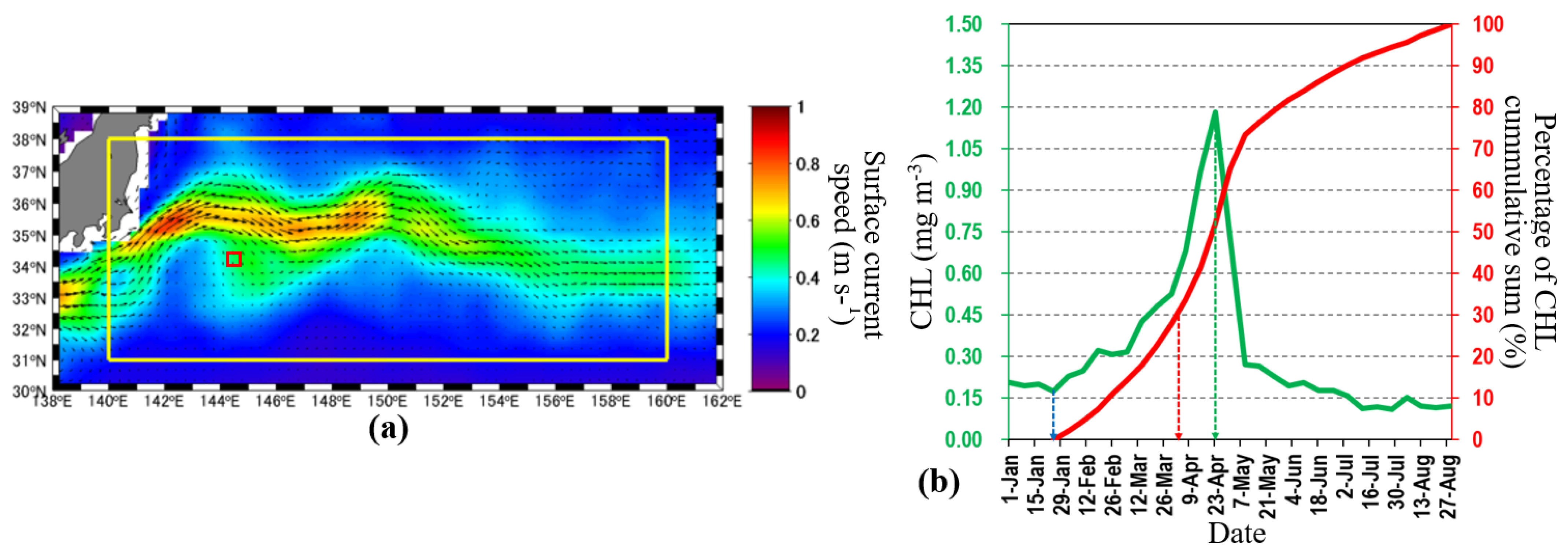
2.1. Study Region

We conducted our study in the western North Pacific Ocean around the region of the KE (31–38°N, 140–160°E) (Figure 1a). Within this study region, the southern (northern) part of the upstream portion of the KE is characterized by a negative (positive) SSHA and high (low) CHL in March–May during the period of unstable (stable) KEs [5,10].

The region is also characterized by an April spring bloom, the onset of which is associated with the cessation of winter mixing and the initiation of water column stratification [14,15]. Because winter deep vertical mixing also reduces light availability within MLD, light availability associated with MLD variation is also important for phytoplankton during the winter [14,18].

2.2. Satellite and Reanalyzed Data

Eight-day mean satellite ocean color CHL data with a 25-km spatial resolution were used to derive temporal variations of phytoplankton biomass. The CHL data were merged data measured by the National Aeronautics and Space Administration (NASA) and European Space Agency multiple ocean color sensors and acquired from the GlobColour Project (https://www.globcolour.info/) (accessed on 21 July 2021). We used daily satellite altimeter-observed SSHA data with a 25-km spatial resolution that were acquired from the Copernicus Marine Service (https://marine.copernicus.eu/) (accessed on 9 April 2021). Eight-day mean SSHA data were created by averaging daily SSHA data during the 8-day periods used to average the CHL data.

Eight-day MLD and sea surface temperature (SST) data were constructed from the 7-day mean MLD and SST data and acquired from the Copernicus Marine Service. The MLD and SST data had a 25 km spatial resolution and were merged products from in situ and satellite observations. We used ocean surface current data generated from multiple satellite observations made by the Ocean Surface Current Analysis Real-Time (OSCAR) Project to visualize the general ocean surface circulation. The ocean surface current data were five-day mean products with a spatial resolution of 1/3 degree and were acquired from the NASA Physical Oceanography Data Center (https://podaac.jpl.nasa.gov/) (accessed on 10 December 2020).

In this study, we used datasets from 1998 to 2017, a time interval that includes the periods of unstable and stable KEs. Besides the availability of datasets during the time of this work, we limited our analysis to the data from 1998 to 2017 for consistent comparison with previous work [5]. The coverage of the aforementioned gridded data is global. Cropping was therefore conducted to create subsets of those data that covered the study region (Figure 1a). To be able to determine the onset of the spring bloom, spatiotemporally no-gap CHL data were required. Interpolation to fill the gaps was thus conducted using an empirical orthogonal function-based data interpolation scheme [19]. We emphasized SSHA and MLD variability in winter (January–March) because physical oceanographic processes during the winter largely determine the intensity and timing of the phytoplankton spring bloom [14,15,18].

2.3. Defining the Spring Bloom Onset

The winter–spring phytoplankton phenology in the areas south of the upstream portion of the KE is characterized mainly by a winter minimum in January and spring bloom peaks in April [14,20]. We applied the cumulative sum (CS) method to the 8-day mean CHL data to define the onset of the spring bloom (Figure 1b). The CHL data were cumulatively summed from the time of the winter minimum CHL to the end of August, and the time at which the value of the sum reached the threshold percentage of the total accumulated CHL at the end of August was defined as the onset of the spring bloom [21,22,23].

Brody et al. [21] suggested that the CS method is more flexible for multiple research purposes than other methods they examined in their study. The CS method is also not affected by the interpolation method used to fill data gaps [21]. The threshold percentages used in previous studies ranged from 10% to 40% [21,22,23]. In this study, the onset of the spring bloom was defined to be the time when the percentage of the CHL cumulative sum reached 30%. The threshold of 30% was used by Brody et al. [21] and Shi et al. [23] to ensure that the procedure had truly detected the onset of the spring bloom. The selected threshold value, however, was not critical to the conclusions of this study (see Discussion).

3. Results

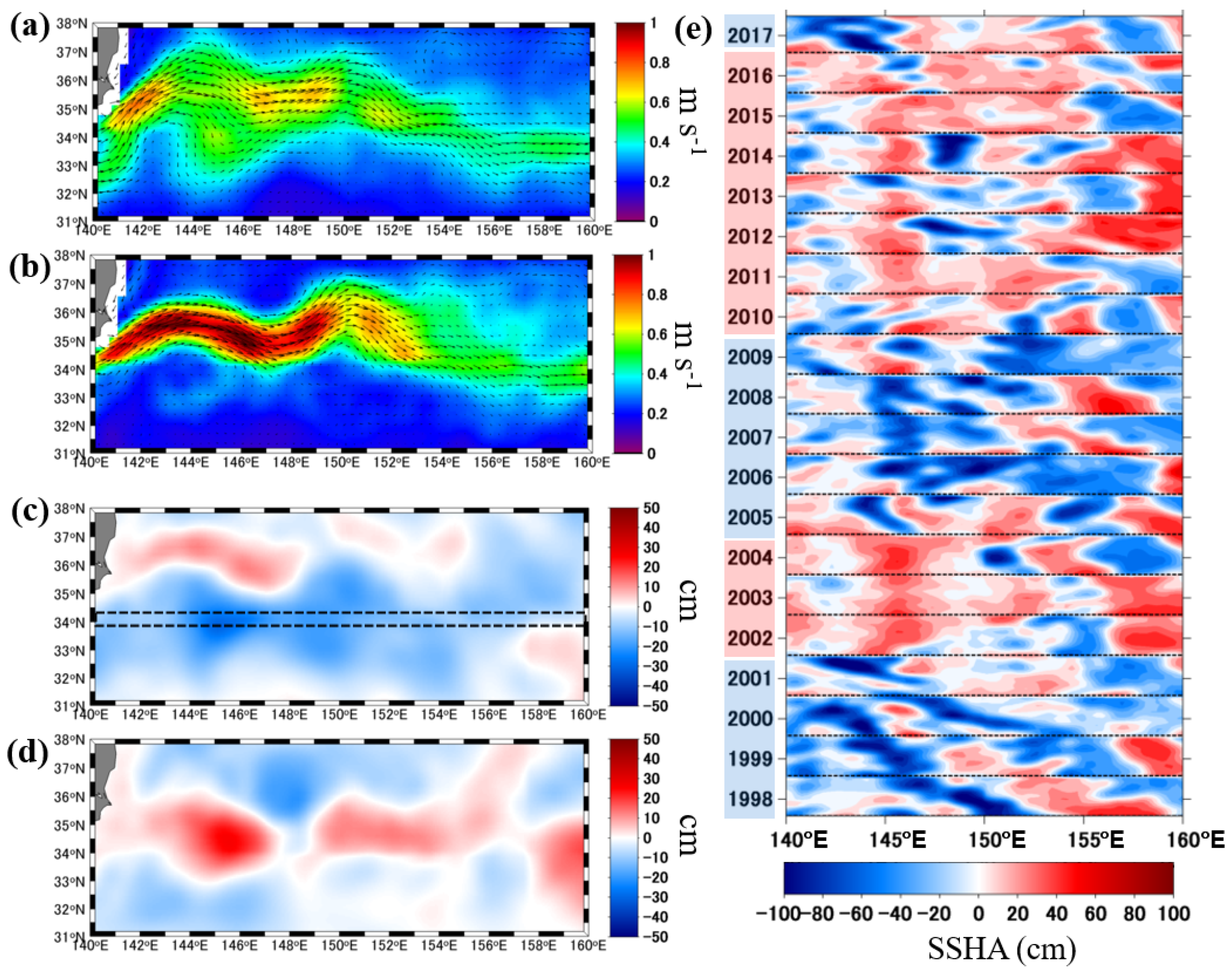
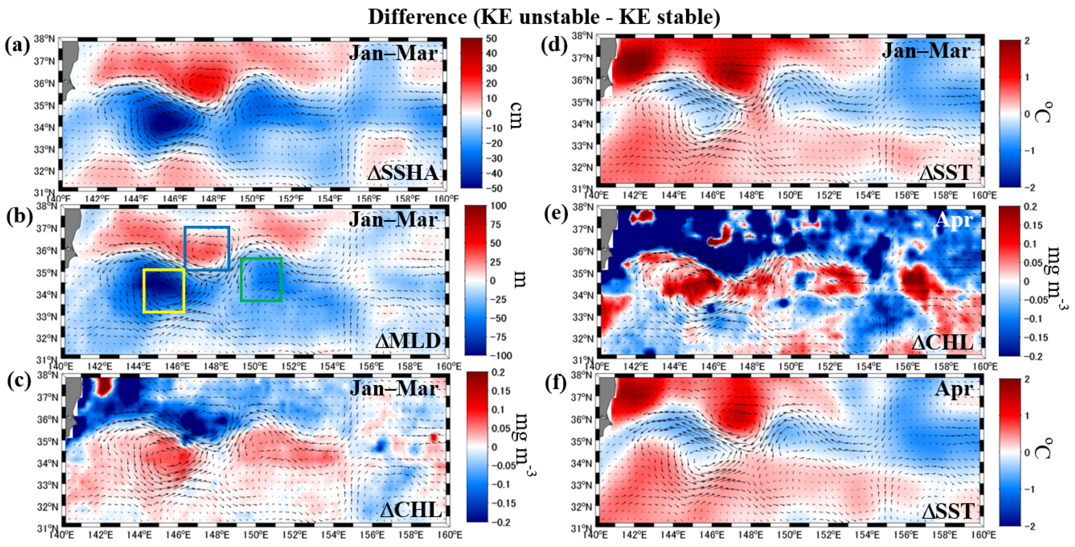
3.1. Biogeophysical Properties during the Periods of Unstable and Stable KEs

During the period of unstable (stable) KEs, the upstream portion of the KE (140–152°E) was characterized by a weak (strong) KE and a broad (narrow) Kuroshio mainstream (Figure 2a,b). Compared to during stable conditions (Figure 2d), SSHA south of the KE during the period of unstable KE was more characterized by negative anomalies (Figure 2c) consistent with the result of the study by Lin et al. [10].

These negative SSHAs south of the KE during the period of unstable KEs were mainly attributed to two physical factors. First is the negative SSHAs that are propagated westward from the central Pacific Ocean and remotely induced by large-scale wind stress curl anomalies associated with the positive phase of PDO or negative phase of NPGO [1,2,3,4]. The second factor is more mesoscale cyclonic eddies generated south of the KE during the period of unstable KEs than during the period of stable KEs [9]. The tendency of positive SSHAs south of the KE during the period of stable KE is thus attributed to the westward propagation of positive SSHAs associated with negative PDO or positive NPGO. Henceforth, we simply define the KE as the Kuroshio mainstream indicated by the strong westward ocean surface current difference (Δcurrent, calculated by subtracting ocean currents during the period of stable KE from the period of unstable KE) and separate the north-south seesaws of biogeophysical variables (Figure 3).

In contrast to the south of the KE, the mean SSHA north (>35°N) of the KE was positive during the unstable KE period. This positive SSHA is attributed to more anticyclonic eddies detached from the KE’s north [7]. As mentioned by Oka et al. [7], westward propagating negative SSHAs from the central Pacific Ocean change to positive anomalies due to active anticyclonic eddy generation.

The SSHAs could then be used to identify KE stabilities. As can be seen from Figure 2e, the KE was unstable (stable) in the winter during the years 1998–2001, 2005–2009, and 2017 (2002–2004 and 2010–2016), and it was characterized by negative (positive) SSHAs. These periods of unstable and stable KEs have been reported in other studies [5,8] and references therein.

Figure 3a shows the winter SSHA difference (ΔSSHA) calculated by subtracting the winter mean SSHA during the years of stable KEs from the winter mean SSHA during the years of unstable KEs (unstable KE minus stable KE SSHAs). Consistent with the result of the study by Lin et al. [5], the ΔSSHA south of the KE was negative simply because more cyclonic eddies are generated during the period of unstable KEs than during the period of stable KEs and the westward propagating SSHAs from the central Pacific Ocean are negative (positive) during the period of unstable (stable) KEs.

Over approximately the same area (south of the KE) where ΔSSHA was negative, a pronounced negative MLD difference (ΔMLD, calculated similarly like ΔSSHA) (Figure 3b) was observed. Such a negative ΔMLD was attributed to Ekman divergences associated with more cyclonic eddies generated during the period of unstable KEs [9]. The negative ΔMLD was also attributed to uplifted (deepened) thermocline during the unstable (stable) period of the KEs [1,5]. An uplift of the thermocline made it easier for winter mixing to entrain cold, nutrient-rich deep water and hence was likely the mechanism responsible for the observed negative difference in winter SST (ΔSST, i.e., unstable KE minus stable KE SSTs) (Figure 3d) in the core areas where the ΔSSHA and ΔMLD were negative.

In contrast, areas north of the KE were characterized by positive ΔSSHAs and ΔSSTs (computed by subtracting mean SST during stable KEs from unstable KEs). This was attributed to the Ekman convergence effect of anticyclonic mesoscale eddies, which were more generated and detached to the north from the KE during the period of unstable KEs [7]. Henceforth, when the adjective “higher” or “lower” describes any variable during the periods of unstable KEs, the adjective means “higher” or “lower” relative to the values of the variables during the periods of stable KEs, and vice versa. The same logic also applies to the adjective “earlier” when it describes the onset of a bloom (i.e., the onset of the bloom was earlier during the period of unstable KEs than during the periods of stable KEs).

Figure 3c shows the difference of the winter CHL (ΔCHL) between the periods of unstable and stable KEs calculated in the same way as the ΔSSHA, ΔMLD, and ΔSST. The positive values of the ΔCHL in the areas where the ΔSSHA and ΔMLD were negative indicated that CHL tended to be high (low) during the periods of unstable (stable) KEs. On average, winter CHL was higher by 15–30% during the periods of unstable KEs. In the areas north of the KE (north of about 36°N), however, the ΔCHLs were negative and were accompanied by positive ΔSSHAs, ΔMLDs, and ΔSSTs.

Over the main areas of positive ΔCHLs south of the KE, the positive ΔCHLs persisted from winter to spring (Figure 3c,e). We also found that in some areas where the ΔCHLs were weakly positive in winter, they turned to negative in April (spring). The indication was, over those areas, the CHLs in spring (Figure 3e) tended to be lower during the KE unstable period than those during the KE stable period. The areas with negative ΔCHLs in spring colocated with the areas with positive ΔSSTs both in winter and spring (Figure 3d,f).

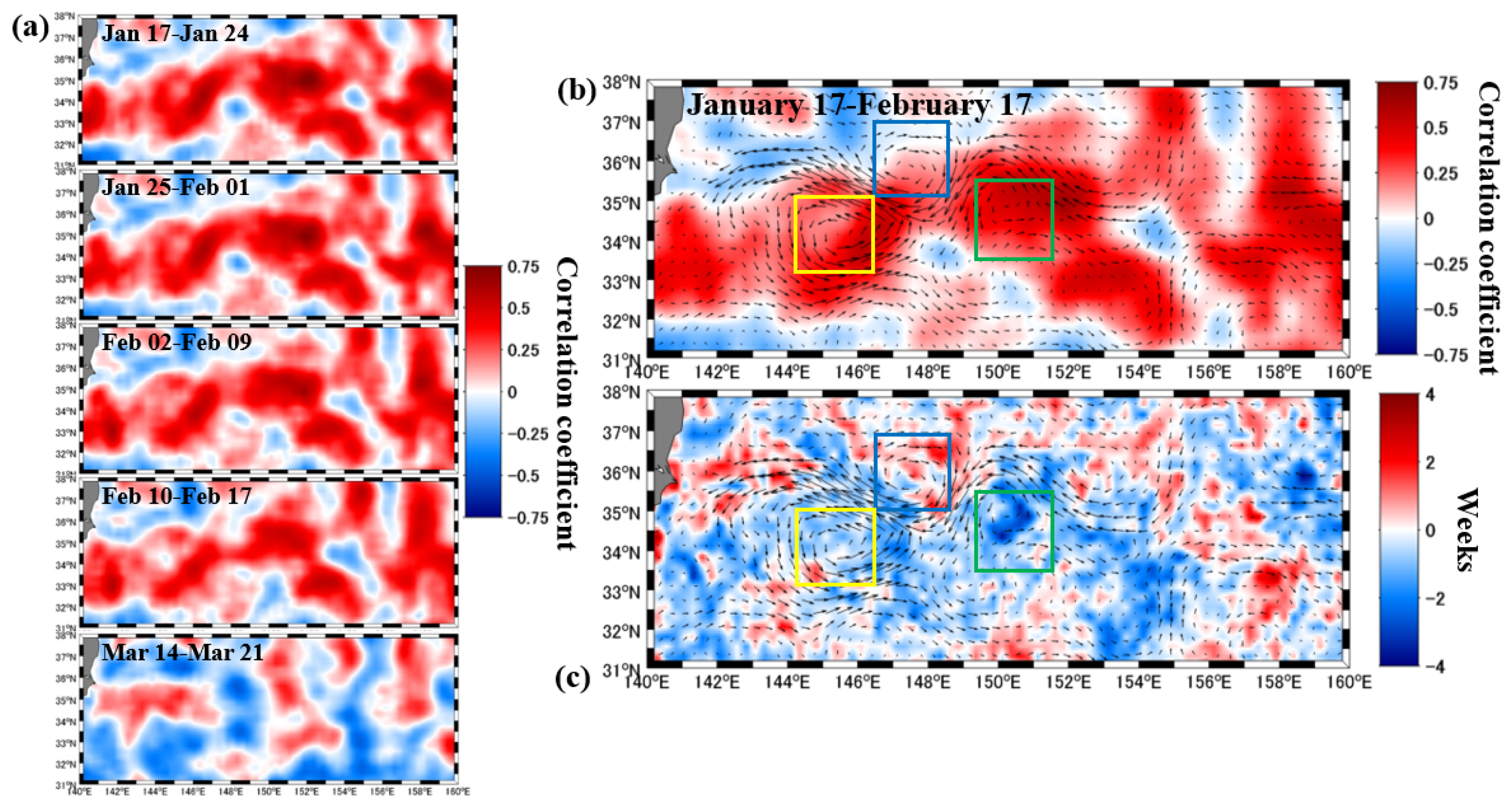
3.2. Relationship between SSHA and Phytoplankton Spring Bloom Onset

One of the research questions to be addressed in this work is whether there is a difference in the spring bloom onset between the periods of unstable and stable KEs which are characterized by negative SSHAs and positive SSHAs, respectively. We hypothesized that if the difference in the bloom onset between the two KE dynamic states is associated with SSHA variation, SSHA should be correlated with the spring bloom onset.

Therefore, we correlated the SSHAs to the onsets of the spring bloom estimated using the CS method. Figure 4a shows maps of the correlation coefficients between the SSHAs and the onsets of the spring bloom, where the SSHAs were averaged over the periods 17–24 January, 25 January–1 February, 2–9 February, 10–17 February, and 14–21 March. The patterns of spatial variation in SSHA–bloom onset correlations shown in Figure 4a were similar, except for the correlation when 14–21 March SSHA data were used (bottom map in Figure 4a). Therefore, correlation derived by using SSHAs data from 17 January to 17 February can be considered to depict the typical relationship between winter SSHAs and the onsets of the phytoplankton spring bloom (Figure 4b).

The positive correlation between SSHA and onset of the spring bloom means that negative SSHAs (due to more cyclonic eddies and negative SSHA westward propagation) during the winter were associated with earlier onsets of the phytoplankton spring bloom. The implication is that during the periods of unstable KEs characterized by negative SSHAs, the onsets of the spring bloom south of the KE tended to be earlier.

Earlier spring bloom onsets mainly south of the KE during the period of unstable KEs were also confirmed by negative differences in spring bloom onsets between the periods of unstable and stable KEs (Δonset, calculated by subtracting mean bloom onset during stable KE period from mean bloom onset during unstable KE period) (Figure 4c). Interestingly, the areas south of the KE which were characterized by negative Δonset (earlier bloom onset during the period of unstable KEs) were approximately located over the same areas showing SSHA-bloom onset positive correlation (Figure 4b), negative ΔSSHA (Figure 3a), and negative ΔMLD (Figure 3b). The aforesaid spatial pattern similarity thus supports our hypothesis that the spring bloom onset during the period of unstable KEs was indeed earlier and such an earlier bloom onset was associated with negative SSHAs. The largest negative Δonset could be 3 weeks (see dark blue areas within the green box in Figure 4c) meaning that the bloom onset during the unstable period of KEs could be 3 weeks (or 24 days) earlier. We could not calculate the Δonset into a daily unit because we used weekly (8-day) mean CHL data.

We extracted data from three areas shown in Figure 3 and Figure 4—two areas (yellow and green boxes) south of the KE and one area (blue box) north of the KE—to facilitate visualization in more detail of the mean temporal variations of CHL, SSHA, and MLD from winter to spring (January–April) during the periods of unstable and stable KEs. There is no specific scientific reason for selecting those areas. The two areas (yellow and green boxes) were selected simply because they are located south of the KE and the core areas of negative ΔSSHA, ΔMLD, and ΔSST. One area denoted by a blue box was selected simply because it is located north of the KE and the core area of positive ΔSSHA, ΔMLD, and ΔSST. In the two areas south of the KE, winter CHL during the period of unstable KEs was higher (Figure 5a,c). Shallower MLDs and more negative SSHAs during the period of unstable KE reflected the more frequent cyclonic eddies generated [9], westward propagation of negative SSHAs [1,2], and uplift of thermocline [5,10] during the period of unstable KEs.

Over the areas south of the KE, the CS method with a 30% threshold [23] yielded Δonset that averaged about 1–2 weeks, meaning that the onset of the spring bloom during the period of unstable KEs was about 1–2 weeks earlier (Figure 5b,d), though it could be 3 weeks, as observed within the green box in Figure 4c. But if a threshold value of 15% [21] was adopted, the onset of the spring bloom during the period of unstable KEs was 2–3 weeks earlier. To eliminate the bias of spring bloom onset due to high winter CHL, we normalized the CHL to values between 0 and 1. From mid-February to mid-March, a value of normalized CHL was reached 1–3 weeks earlier during the period of unstable KEs than during the period of stable KEs. Whereas the winter CHL during the period of unstable KEs tended to be higher, it is also possible to observe the spring bloom CHL magnitude to be lower during the period of unstable KEs (Figure 5a–d, see also negative ΔCHL in spring south of KE in Figure 3e).

The Δonset is not as obvious in the areas north of the KE as it is to the south of the KE (Figure 5e,f). The tendency of the impact of the eddies on the onset of the spring bloom to not be as strong north of the KE as south of the KE can also be seen from the weak correlation between winter SSHA and the onset of the bloom (Figure 4). It is obvious, however, that, compared to the areas south of the KE, the peak of the spring bloom north of the KE is much lower during the period of unstable KEs (Figure 5e,f).

4. Discussion

As shown in Figure 3c and Figure 5a–d, winter CHLs south of the KE during the period of unstable KEs were relatively higher. As mentioned by Lin et al. [5], such a higher CHL during the period of unstable KEs can be attributed to increased nutrients due to the uplift of nitracline associated with westward propagation of negative SSHAs from the central Pacific Ocean [1,2]. The uplift of the nitracline eases the entrainment of nutrients from the deep layer to the euphotic layer. The entrained nutrients then promote phytoplankton growth during the spring [5] as nutrients are the main limiting factors. Southward advection of high CHL waters from the KE due to more cyclonic eddy generation might also be one of the factors [9]. Especially during the winter, with plenty of nutrients entrained by winter vertical mixing, the shallower MLD (Figure 3b and Figure 5a–d, due to the uplift of thermocline and the effect of Ekman divergence) might also be an important factor in the increase of winter CHL. This is because shallow MLD will prevent phytoplankton to be mixed into a low-light deep layer, hence will increase light availability within the mixed layer. Previous works indeed mentioned that light is important for phytoplankton during the winter in this region [14,18]. Mahadevan et al. [16] also mentioned that by increasing the light exposure of phytoplankton, mesoscale eddy-driven stratification increases winter primary production in the North Atlantic Ocean.

Over the main areas south of the KE where ΔSSTs are negative from January to April (Figure 3d,f), ΔCHLs were positive (Figure 3c,e), which is consistent with the results of the study by Lin et al. [5]. Over these negative ΔSST areas, the negative ΔSST observed since winter means much more amount of cold, hence nutrient-rich, deep water reached the surface layer during the period of unstable KEs due to active winter vertical mixing in addition to other physical processes such as the uplift of the nitracline and cyclonic eddy formation. Previous works [5,11,24,25,26] mentioned that the amount of nutrients supplied during the winter plays a very important role in modulating the magnitude of the phytoplankton spring bloom. The above mechanism thus explains the more prominent positive ΔCHLs in April (Figure 3e).

However, over the south of the KE where ΔSSTs were positive (i.e., warmer SSTs during unstable KEs) from January to April, the ΔCHLs in spring were negative (see blue patches south of about 34°N in Figure 3e), indicating that April CHLs tended to be lower during the period of unstable KEs. Further study is needed to understand the mechanisms responsible for the lower CHLs during unstable KEs over the positive ΔSST areas. Warmer SSTs during unstable KEs that affect nutrient supply from the deep layer might be one of the initial clues for future study.

Previous studies [14,15,20] have used slightly different explanations to suggest that physical processes that dampen winter vertical mixing, strengthen vertical stratification, and weaken winter turbulence ultimately improve light conditions for phytoplankton growth and are important determinants of the onset of the spring bloom. Although the aforesaid physical factors are not necessarily associated with shoaling of the mixed layer, a shallow MLD increases the exposure of phytoplankton to light within the mixed layer. Previous works [16,17] mentioned that the increased exposure of phytoplankton to light caused by shoaling of the mixed layer and strengthening of water column stratification advances the onset of the phytoplankton spring bloom in the North Atlantic Ocean and Japan Sea, respectively. We thus adopted a similar mechanism (i.e., shallower MLD during unstable KEs) that increased light availability within the MLD to cause the earlier onset of the spring bloom south of the KE during the period of unstable KEs.

In the areas north of the KE, CHLs in the spring during the period of unstable KEs were much lower (Figure 5e,f). The positive ΔSST north of the KE from winter to spring (Figure 3d,f) indicates that the SST is relatively warm (and the nitracline deep) during the period of unstable KEs because of greater activity of anticyclonic eddies detached from the KE [7]. Because of the anticyclonic eddy’s Ekman divergence effect, both a deep nitracline (in winter) and warm SST (in spring) make the nutrients in deeper layers hard to entrain into the surface layer. The low supply of nutrients in the winter–spring then causes the CHL spring bloom peak to be remarkably low during the period of unstable KEs.

Depending on the threshold values used to define the onset of the spring bloom, the onset of the spring bloom south of the KE during the period of unstable KEs can be 1–3 weeks earlier (Figure 5a–d). Statistically, the 1–3 week difference of the onset of the spring bloom might or might not be significant. The most important scientific question to be addressed is whether that difference has a significant ecological impact on the higher-trophic-level marine organisms. Kodama et al. [12] found that the onset of the phytoplankton spring bloom is more important than the duration and magnitude of the spring bloom in controlling Japanese sardine recruitment in the Sea of Japan. They found that there is a significant positive correlation between the onset of the spring bloom and Japanese sardine recruitment, i.e., an early (late) onset of the spring bloom worsens (improves) recruitment of Japanese sardines. Similarly, in the KE region, Nishikawa and Yasuda [13] found that the early onset of the phytoplankton spring bloom, which is also associated with a shallow winter MLD, decreases the population of Japanese sardines. They also suggested that the earlier onset of the bloom due to a shallow winter MLD reduces the spring phytoplankton biomass and leads to an insufficient supply of food in the spring for Japanese sardine larvae and juveniles. The first part of this scenario is consistent with our analysis. Whether there is less successful recruitment of Japanese sardines during the period of unstable KEs (i.e., less sardine recruitment due to earlier onset of the spring bloom in association with the shallow winter MLD) is worth investigating in future studies.

5. Conclusions

We used satellite datasets from the period 1998–2017 to investigate the phenology of phytoplankton during the winter–spring in association with the instability of the KE. In the areas south of the KE, CHL in winter tended to be high during the period of unstable KEs. Besides the increase in nutrients due to well-known physical processes associated with the decadal oscillations in the central Pacific Ocean, the increase in the exposure of phytoplankton to light within the mixed layer due to shallower MLD was also considered important to cause higher CHLs during the period of unstable KEs.

In spring, the CHLs south of KE during the period of unstable KEs can be higher or lower than during the period of stable KEs. The areas where the spring CHL was higher were associated with a large supply of nutrients during the winter–spring driven by physical processes already discussed. The detailed mechanisms responsible for the lower CHLs in spring during the period of unstable KEs need to be studied in future works, but the warmer SSTs (reduced nutrient supply from deep layer) in winter–spring during the period of unstable KEs might be an initial clue.

Mainly to the south of the KE, the instability of the KE also modified the onset of the spring bloom. On average, the onset of the spring bloom tended to be 1–3 weeks earlier during the period of unstable KEs than during the period of stable KEs. Whether this onset of the bloom 1–3 weeks earlier (later) during the period of unstable (stable) KEs influence the higher trophic-level marine organism recruitment is worth investigating in future studies.

References

1. Qiu, B. Kuroshio Extension variability and forcing of the Pacific decadal oscillations: Responses and potential feedback. J. Phys. Oceanogr. 2003, 33, 2465–2482. [Google Scholar] [CrossRef]
2. Qiu, B.; Chen, S. Variability of the Kuroshio Extension jet, recirculation gyre, and mesoscale eddies on decadal time scales. J. Phys. Oceanogr. 2005, 35, 2090–2102. [Google Scholar] [CrossRef]
3. Taguchi, B.; Xie, S.-P.; Schneider, N.; Nonaka, M.; Sasaki, H.; Sasai, Y. Decadal variability of the Kuroshio Extension: Observations and Eddy-resolving model hindcast. J. Clim. 2007, 20, 2357–2377. [Google Scholar] [CrossRef] [Green Version]
4. Mantua, N.J.; Hare, S.R.; Zhang, Y.; Wallace, J.M.; Francis, R.C. A Pacific interdecadal climate oscillation with impacts on salmon production. Bull. Am. Meteorol. Soc. 1997, 78, 1069–1080. [Google Scholar] [CrossRef]
5. Lin, P.; Ma, J.; Chai, F.; Xiu, P.; Liu, H. Decadal variability of nutrients and biomass in the southern region of Kuroshio Extension. Prog. Oceanogr. 2020, 188, 102441. [Google Scholar] [CrossRef]
6. Di Lorenzo, E.; Schneider, N.; Cobb, K.; Franks, P.; Chhak, K.; Miller, A.; Mcwilliams, J.; Bograd, S.; Arango, H.; Curchitser, E.; et al. North Pacific Gyre Oscillation links ocean climate and ecosystem change. Geophys. Res. Lett. 2008, 35, L08607. [Google Scholar] [CrossRef] [Green Version]
7. Oka, E.; Qiu, B.; Kouketsu, S.; Uehara, K.; Suga, T. Decadal seesaw of the Central and Subtropical Mode Water formation associated with the Kuroshio Extension variability. J. Oceanogr. 2012, 68, 355–360. [Google Scholar] [CrossRef]
8. Yang, H.; Qiu, B.; Chang, P.; Wu, L.; Wang, S.; Chen, Z.; Yang, Y. Decadal variability of eddy characteristics and energetics in the Kuroshio Extension: Unstable versus stable states. J. Geophys. Res. Oceans 2018, 123, 6653–6669. [Google Scholar] [CrossRef]
9. Kouketsu, S.; Kaneko, H.; Okunishi, T.; Sasaoka, K.; Itoh, S.; Inoue, R.; Ueno, H. Mesoscale eddy effects on temporal variability of surface chlorophyll a in the Kuroshio Extension. J. Oceanogr. 2016, 72, 439–451. [Google Scholar] [CrossRef]
10. Lin, P.; Chai, F.; Xue, H.; Xiu, P. Modulation of decadal oscillation on surface chlorophyll in the Kuroshio Extension. J. Geophys. Res. Oceans 2014, 119, 187–199. [Google Scholar] [CrossRef]
11. Nishikawa, H.; Yasuda, I.; Komatsu, K.; Sasaki, H.; Sasai, Y.; Setou, T.; Shimizu, M. Winter mixed layer depth and spring bloom along the Kuroshio front: Implications for the Japanese sardine stock. Mar. Ecol. Prog. Ser. 2013, 487, 217–229. [Google Scholar] [CrossRef] [Green Version]
12. Kodama, T.; Wagawa, T.; Ohshimo, S.; Morimoto, H.; Iguchi, N.; Fukudome, K.; Goto, T.; Takahashi, M.; Yasuda, T. Improvement in recruitment of Japanese sardine with delays of the spring phytoplankton bloom in the Sea of Japan. Fish. Oceanogr. 2018, 27, 289–301. [Google Scholar] [CrossRef]
13. Nishikawa, H.; Yasuda, I. Japanese sardine (Sardinops melanostictus) mortality in relation to the winter mixed layer depth in the Kuroshio Extension region. Fish. Oceanogr. 2008, 17, 411–420. [Google Scholar] [CrossRef]
14. Siswanto, E.; Matsumoto, K.; Honda, M.C.; Fujiki, T.; Sasaoka, K.; Saino, T. Reappraisal of meridional differences of factors controlling phytoplankton biomass and initial increase preceding seasonal bloom in the northwestern Pacific Ocean. Remote Sens. Environ. 2015, 159, 44–56. [Google Scholar] [CrossRef] [Green Version]
15. Matsumoto, K.; Sasai, Y.; Sasaoka, K.; Siswanto, E.; Honda, M.C. The formation of subtropical phytoplankton blooms is dictated by water column stability during winter and spring in the oligotrophic Northwestern North Pacific. J. Geophys. Res. Oceans 2021, 126, e2020JC016864. [Google Scholar] [CrossRef]
16. Mahadevan, A.; D’Asaro, E.; Lee, C.; Perry, M.J. Eddy-driven stratification initiates North Atlantic spring phytoplankton blooms. Science 2016, 337, 54–58. [Google Scholar] [CrossRef]
17. Maúre, E.R.; Ishizaka, J.; Sukigara, C.; Mino, Y.; Aiki, H.; Matsuno, T.; Tomita, H.; Goes, J.I.; Gomes, H.R. Mesoscale eddies control the timing of spring phytoplankton blooms: A case study in the Japan Sea. J. Geophys. Res. Oceans 2017, 44, 11115–11124. [Google Scholar] [CrossRef]
18. Matsumoto, K.; Honda, M.C.; Sasaoka, K.; Wakita, M.; Kawakami, H.; Watanabe, S. Seasonal variability of primary production and phytoplankton biomass in the western Pacific subarctic gyre: Control by light availability within the mixed layer. J. Geophys. Res. Oceans 2014, 119, 6523–6534. [Google Scholar] [CrossRef]
19. Alvera-Azcárate, A.; Barth, A.; Rixen, M.; Beckers, J.-M. Reconstruction of incomplete oceanographic data sets using Empirical Orthogonal Functions. Application to the Adriatic Sea. Ocean Model. 2005, 9, 325–346. [Google Scholar] [CrossRef] [Green Version]
20. Shiozaki, T.; Ito, S.I.; Takahashi, K.; Saito, H.; Nagata, T.; Furuya, K. Regional variability of factors controlling the onset timing and magnitude of spring algal blooms in the northwestern North Pacific. J. Geophys. Res. Oceans 2014, 119, 253–265. [Google Scholar] [CrossRef]
21. Brody, S.R.; Lozier, M.S.; Dunne, J.P. A comparison of methods to determine phytoplankton bloom initiation. J. Geophys. Res. Oceans 2013, 118, 2345–2357. [Google Scholar] [CrossRef]
22. Chiba, S.; Batten, S.; Sasaoka, K.; Sasai, Y.; Sugisaki, H. Influence of the Pacific Decadal Oscillation on phytoplankton phenology and community structure in the western North Pacific. Geophys. Res. Lett. 2012, 39, L15603. [Google Scholar] [CrossRef]
23. Shi, J.; Liu, Y.; Mao, X.; Guo, X.; Wei, H.; Gao, H. Interannual variation of spring phytoplankton bloom and response to turbulent energy generated by atmospheric forcing in the central Southern Yellow Sea of China: Satellite observations and numerical model study. Cont. Shelf Res. 2017, 143, 257–270. [Google Scholar] [CrossRef]
24. Goes, J.I.; Gomes, H.R.; Limsakul, A.; Saino, T. The influence of large-scale environmental changes on carbon export in the North Pacific Ocean using satellite and shipboard data. Deep-Sea Res. II 2004, 51, 247–279. [Google Scholar] [CrossRef]
25. Siswanto, E.; Honda, M.C.; Matsumoto, K.; Sasai, Y.; Fujiki, T.; Sasaoka, K.; Saino, T. Sixteen-year phytoplankton biomass trends in the northwestern Pacific Ocean by the SeaWiFS and MODIS ocean color sensors. J. Oceanogr. 2016, 71, 479–489. [Google Scholar] [CrossRef]
26. Honda, M.C.; Sasai, Y.; Siswanto, E.; Kuwano-Yoshida, A.; Aiki, H.; Cronin, M.F. Impact of cyclonic eddies and typhoons on biogeochemistry in the oligotrophic ocean based on biogeochemical/physical/meteorological time-series at station KEO. Prog. Earth Planet. Sci. 2018, 5, 42. [Google Scholar] [CrossRef]
Figure 1. (a) Overall mean (1998–2017) ocean surface current map based on Ocean Surface Current Analysis Real-Time data. The yellow box shows the study region. (b) Example of data showing a temporal variation of chlorophyll-a concentrations (CHL) (green line) from winter to summer 2001 derived from the station (34°N, 144.5°E) indicated by the red box in (a). The red line in (b) is the CHL cumulative sum in percentage relative to the maximum cumulative sum of CHL by the end of August. Blue, red, and green dashed arrows in (b) indicate the dates of the winter CHL minimum, the onset of the spring bloom (percentage of cumulative sum = 30%), and spring bloom peak, respectively.
Remotesensing 14 01186 g001
Figure 2. The winter (January–March) ocean surface currents in the study region based on Ocean Surface Current Analysis Real-Time data during the periods of unstable Kuroshio Extensions (KEs) (a) and periods of stable KEs (b). Panels (c,d) are the same as panels (a,b), except they show the sea surface height anomalies (SSHAs). Panel (e) shows the time series (1998–2017) of winter SSHAs averaged within the area indicated by the black dashed box in (c). The labeled years (y-axis) in (e), highlighted by the blue and red colors, are the periods when the KE experienced unstable and stable conditions, respectively.
Remotesensing 14 01186 g002
Figure 3. (a) Average difference of winter (January–March) sea surface height anomalies (ΔSSHA) during the periods of unstable and stable Kuroshio Extensions (KEs) calculated by subtracting mean SSHA during years of stable KEs from the mean SSHA during years of unstable KEs. Panels (bd) are the same as (a), except that they show differences in mixed layer depth (ΔMLD), chlorophyll-a concentration (ΔCHL), and sea surface temperature (ΔSST), respectively. Panels (e,f) are ΔCHL and ΔSST, respectively for April. Vectors in (af) represent the average difference of the ocean surface currents based on Ocean Surface Current Analysis Real-Time data during periods of unstable and stable KEs. The yellow, green, and blue boxes are the same as those in Figure 4b,c and represent the areas from which the data were extracted to be shown in Figure 5.
Remotesensing 14 01186 g003
Figure 4. Maps of correlation coefficients between winter sea surface height anomalies (SSHAs) and onsets of the spring bloom. In (a) from top to bottom, analyses were conducted using mean SSHAs observed during 17–24 January, 25 January–1 February, 2–9 February, 10–17 February, and 14–21 March. Panel (b) is the same as (a), except that the SSHAs were averaged from 17 January to 17 February. Panel (c) is the mean spring bloom onset difference (Δonset) between the periods of unstable and stable Kuroshio Extensions (KEs) calculated by subtracting mean spring bloom onset during years of stable KEs from the mean spring bloom onset during years of unstable KEs. Vectors overplotted on (b,c) are winter (January–March) ocean surface current differences between the periods of unstable and stable Kuroshio Extensions (KEs) based on Ocean Surface Current Analysis Real-Time data. The yellow, green, and blue boxes shown in panels (b,c) represent the areas from which the data were extracted to be shown in Figure 5.
Remotesensing 14 01186 g004
Figure 5. (a) Winter–spring mean temporal variations of chlorophyll-a concentrations (CHL) (solid lines with data symbols), mixed layer depth (MLD) (dashed lines), and sea surface height anomalies (SSHA) (dotted lines) averaged over the region indicated by the yellow box in Figure 4b,c. The blue and red lines indicate the data during the unstable and stable periods of the Kuroshio Extension (KE), respectively (see Figure 2e for the years of unstable and stable KEs). (b) CHL data as in (a) overplotted with their cumulative sum in percentage (dashed lines). Panels (c,d) and (e,f) are the same as panels (a,b) except that they were derived from the regions indicated by green and blue boxes, respectively, shown in Figure 4b,c. The blue (red) downward arrows in (b,d,f) indicate the onsets of the spring bloom defined, respectively, by 15 and 30% thresholds during the periods of unstable (stable) KEs.
Remotesensing 14 01186 g005
Publisher’s Note: MDPI stays neutral with regard to jurisdictional claims in published maps and institutional affiliations.