Correlation-Guided Ensemble Clustering for Hyperspectral Band Selection

Abstract

Hyperspectral band selection is a commonly used technique to alleviate the curse of dimensionality. Recently, clustering-based methods have attracted much attention for their effectiveness in selecting informative and representative bands. However, the single clustering algorithm is used in most of the clustering-based methods, and the neglect of the correlation among adjacent bands in their clustering procedure is prone to resulting in the degradation of the representativeness of the selected band set. This may, consequently, adversely impact hyperspectral classification performance. To tackle such issues, in this paper, we propose a correlation-guided ensemble clustering approach for hyperspectral band selection. By exploiting ensemble clustering, more effective clustering results are expected based on multiple band partitions given by base clustering with different parameters. In addition, given that adjacent bands are most probably located in the same cluster, a novel consensus function is designed to construct the final clustering partition by performing an agglomerative clustering. Thus, the performance of our addressed task (band selection) is further improved. The experimental results on three real-world datasets demonstrate that the performance of our proposed method is superior compared with those of state-of-the-art methods.

1. Introduction

Hyperspectral remote sensing images (HSIs) contain rich spectral and spatial information of ground objects. Thus, they are widely used in land cover classification [1,2], environmental protection [3], mineral exploration [4], precision agriculture [5], and other fields [6,7]. In these fields, hyperspectral classification is an important application that can identify different materials with subtle spectral divergences. However, there is much redundant information in hyperspectral image cubes because of the strong correlations among adjacent bands, which cause Hughes’ phenomenon [8]. This may deteriorate the performance of hyperspectral classification [9]. Therefore, reducing the dimensionality of HSIs before classification is necessary.

The dimensionality reduction techniques of HSIs mainly include feature extraction [10,11,12] and band selection [13,14,15,16,17,18,19,20]. Compared with feature extraction, which maps high-dimensional data into a low-dimensional space, band selection methods can select a subset of representative bands from all bands and thus can well retain the original physical meaning of HSIs [9]. According to whether there are labeled samples, band selection methods can be classified as supervised [13], semi-supervised [14], and unsupervised [15,16,17,18,19,20]. Due to the high cost of obtaining labeled samples, supervised and semi-supervised methods are difficult to apply in practical applications. In contrast, unsupervised methods do not require labeled samples and thus can be better applied in real tasks [18].

Unsupervised band selection methods can be further categorized into ranking-based, sparsity-based, searching-based, and clustering-based methods. Ranking-based methods, such as maximum-variance principal components analysis (MVPCA) [16] and manifold ranking-based method [21], perform band selection by assigning a weight to each band using some criteria and then selecting the top-ranked bands. As the ranking-based methods neglect the correlation between bands, the selected bands may have considerable information redundancy [22]. Sparsity-based methods, such as sparse non-negative matrix factorization [23] and low-rank representation [24], select proper bands by fully exploiting the sparsity representation of hyperspectral bands. However, the global structure information of HSIs is hard to capture effectively in the learned sparse coefficient matrix, limiting the effectiveness of the band selection of sparsity-based methods [25]. Searching-based methods, such as the firefly algorithm [26] and particle swarm optimization algorithm [27], select representative bands by optimizing a given criterion. However, the computational complexity of the nonlinear search process involved in these methods is relatively high [28]. Clustering-based methods have attracted much attention due to the low redundancy of their selected bands and their high classification accuracy [15]. These methods, such as Ward’s linkage strategy using divergence (WaluDi) [17], normalized cut-based optimal clustering with ranking criteria using information entropy (NC-OC-IE) [18], and adaptive subspace partition strategy (ASPS) [19], first divide all bands into multiple clusters, and then select the most representative band in each cluster. Recently, Zeng et al. [29] proposed a deep subspace clustering (DSC), which combined the subspace clustering into a convolutional autoencoder to obtain more accurate clustering results. Although clustering-based methods have improved the effectiveness of band selection to some extent, they also have some shortcomings in the clustering process. For example, most of these methods use a single clustering algorithm, which may be sensitive to the randomly chosen initial centroids. Thus, the effectiveness and robustness of clustering results cannot be guaranteed for high-dimensional data [15,16,17]. In addition, most clustering-based methods neglect the exploitation of problem-dependent information of band selection during clustering.

In recent years, ensemble clustering has attracted extensive attention as it can combine multiple base partitions into a more effective clustering. Moreover, ensemble clustering has shown advantages in generating a robust partition, dealing with noisy features, and mining novel structures [30,31]. Generally, ensemble clustering can be classified into objective function-based and heuristic-based methods [30]. The objective function-based methods treat the similarity measures between partitions as an explicit global objective for designing an effective consensus function. Representative methods include combination regularization [32] and K-means-like algorithm [33]. In contrast, heuristic-based methods, such as voting-based [34] and co-association matrix-based methods [31], employ some heuristics instead of objective functions to search for approximate solutions. For example, Huang et al. [31] recently proposed a locally weighted ensemble clustering method, which estimated the uncertainty for each cluster of all the base clusterings by entropy theory to further improve the consensus clustering results by exploiting a locally weighted strategy in the consensus function. Although the existing ensemble clustering methods have made significant improvements in clustering performance, they have not been fully tested for band selection tasks. In addition, these methods were developed without considering the inherent characteristics of HSIs. Therefore, introducing problem-dependent information of hyperspectral band selection into the clustering strategy and designing an effective consensus function for generating superior consensus clustering results remains challenging.

Aiming to select more representative bands from HSIs by improving the accuracy of clustering, in this paper, we propose a novel correlation-guided ensemble clustering (CGEC) approach for hyperspectral band selection. By exploiting ensemble clustering in our work, more effective clustering results are expected based on multiple band partitions respectively obtained by K-means methods with different parameter settings. In practice, adjacent bands have a strong correlation because of the continuity of the bands in HSIs [19]. To effectively exploit this property of HSIs in ensemble clustering, the proposed CGEC approach incorporates the similarity relationship between adjacent bands into the design of a consensus function for ensemble clustering. Consequently, the clustering results yielded by the proposed CGEC better satisfy the needs of band selection applications. Specifically, multiple initial base clustering results are first obtained by setting diverse parameters for K-means. Then, a novel consensus function is proposed to act as a consensus strategy for generating consensus clustering results by considering the assumption that adjacent bands most probably located in the same cluster [18]. Then, the target bands are obtained by adopting an improved manifold ranking method that selects a representative band from each cluster. In our experiments, the proposed approach is compared with seven representative competitors on three real hyperspectral datasets. The experimental results show the superiority of our proposed method.

2. Method

2.1. Ensemble Clustering

Clustering aims to divide similar data into several clusters using a certain dissimilarity measure without prior knowledge. When a clustering method is performed on high-dimensional datasets, traditional clustering methods such as K-means and spectral clustering may be challenging [35]. Ensemble clustering is an emerging approach that can provide more accurate and robust clustering results based on multiple data partitions given by base clustering [36]. The formal description of ensemble clustering can be expressed as follows.

Given a set of N data patterns $O=\left\{{\mathbf{o}}_1,{\mathbf{o}}_2,\cdots ,{\mathbf{o}}_N\right\}$, after running the base clustering algorithm Z times, the partitions obtained by all the base clustering algorithms form a set $\mathsf{\Pi }=\left\{{\pi }^1,{\pi }^2,\cdots ,{\pi }^z,\cdots ,{\pi }^Z\right\}$, where ${\pi }^z=\left\{G_1^z,G_2^z,\cdots ,G_{n^z}^z\right\}$, referred to as base clustering, is the z-th partition that divides O into $n^z$ crisp clusters, and maps each data point of O to a cluster label (ranging from 1 to $n^z$). The consensus partition ${\pi }^{*}$ given by ensemble clustering is defined as follows

$${\pi }^{*}=g\left(\mathsf{\Pi }\right)=\left\{G_1^{*},G_2^{*},\cdots ,G_l^{*},\cdots ,G_L^{*}\right\},$$

(1)

where $G_l^{*}$ denotes the l-th cluster given by ensemble clustering, and $g(·)$ represents a consensus function that generates the consensus partition based on all the base clusterings.

2.2. Locally Weighted Ensemble Clustering

In ensemble clustering, low-quality base clusterings may seriously affect the results of ensemble clustering. To address this issue, a locally weighted ensemble clustering (LWEC) method has recently been proposed [31], which develops the uncertainty estimation and validity measurement for each cluster of all the base clusterings to improve the consensus performance. Specifically, LWEC integrates the uncertainty and validity of each cluster into the locally weighted strategy to generate a locally weighted co-association (LWCA) matrix that is used to indicate the probability that two objects are divided into the same cluster among the multiple base clusterings. The cluster uncertainty is measured by exploiting the entropy theory, whereas the cluster validity is evaluated using an ensemble-driven cluster index (ECI), which will be explained in Equation (5) below. According to the ECI, LWEC constructs an LWCA matrix as a summary of the diverse clusters of all the base clusterings.

More precisely, LWEC uses the concept of entropy to measure the uncertainty of each cluster, which indicates the difference that the objects of a cluster are partitioned among multiple base clusterings. Formally, given a cluster $G_i\in {\pi }^z$, the entropy of $G_i$ w.r.t. the base clustering ${\pi }^z$ (z=1, 2, ⋯, Z) is defined as

$$H^z\left(G_i\right)=-\sum _{j=1}^{n^z}f\left(G_i,G_j^z\right){log}_{2}f\left(G_i,G_j^z\right),$$

(2)

with

$$f\left(G_i,G_j^z\right)=\frac{\left|G_i\cap G_j^z\right|}{\left|G_i\right|},$$

(3)

where $n^z$ denotes the number of clusters included in ${\pi }^z$ and $G_j^z$ represents the j-th cluster of ${\pi }^z$. The symbol $”\cap “$ expresses the intersection of two clusters, and $|G_i|$ indicates the number of objects in $G_i$. On the basis of Equation (2), the entropy of cluster $G_i$ w.r.t. the set of base clusterings $\mathsf{\Pi }$ is defined as

$$H^{\mathsf{\Pi }}\left(G_i\right)=\sum _{z=1}^Z{H}^z\left(G_i\right),$$

(4)

where Z denotes the number of base clusterings in $\mathsf{\Pi }$.

ECI is proposed to measure the validity of each cluster of all the base clusterings by considering the entropy of each cluster w.r.t. the set of base clusterings. More formally, given the set of base clusterings $\mathsf{\Pi }$ with Z base clusterings, ECI for the cluster $G_i$ is defined as

$$ECI\left(G_i\right)=exp\left(-\frac{H^{\mathsf{\Pi }}\left(G_i\right)}{\theta ·Z}\right),$$

(5)

where $\theta$ denotes a parameter used to adjust the influence of the entropy over ECI. According to Equation (5), obviously, the smaller the entropy of a cluster $G_i$, the greater the value of $ECI\left(G_i\right)$. Based on ECI, the LWCA matrix is constructed to reflect the probability that two objects are divided into the same cluster among the multiple base clusterings. Formally, the LWCA matrix $\mathbf{W}$ is defined as

$$\mathbf{W}=\left({\mathbf{w}}_{ij}\right)\in {\mathbb{R}}^{N\times N},$$

(6)

with

$${\mathbf{w}}_{ij}=\frac{1}{Z}·\sum _{z=1}^Z{v}_i^z·r_{ij}^z,$$

(7)

$$v_i^z=ECI\left(Gl{s}^z\left({\mathbf{o}}_i\right)\right),$$

(8)

$$r_{ij}^z=\left\{\begin{array}{cc}1,\hfill & \mathrm{if}Gl{s}^z\left({\mathbf{o}}_i\right)=Gl{s}^z\left({\mathbf{o}}_j\right)\hfill \\ 0,\hfill & \mathrm{otherwise}\hfill \end{array},\right.$$

(9)

where $Gl{s}^z\left({\mathbf{o}}_i\right)$ denotes the cluster in which an object ${\mathbf{o}}_i$ belongs. To generate the clustering results of ensemble clustering, LWEC exploits locally weighted evidence accumulation (LWEA) as a consensus function, which is used to guide the merging of two clusters in the hierarchical agglomerative clustering. Note that LWEA is developed without considering the characteristics of hyperspectral data and not tested on the task of band selection.

2.3. CGEC

The flowchart of our proposed approach is illustrated in Figure 1. This approach consists of two parts: ensemble clustering and manifold ranking. Via ensemble clustering, multiple base partitions given by a group of base clustering algorithms can be combined into a more effective and robust partition with the help of an effective consensus function. Next, the manifold ranking method is used to generate representative bands based on the clustering results given by the ensemble clustering. Specifically, in the part of ensemble clustering, given the HSI data $\mathbf{B}\in {\mathbb{R}}^{N\times P}$, where N denotes the number of bands and P stands for the number of pixels, we first conduct clustering analysis on $\mathbf{B}$ by running K-means Z times with different parameters in each run. Consequently, the collection of Z base clusterings $\mathsf{\Pi }=\left\{{\pi }^1,{\pi }^2,\cdots ,{\pi }^z,\cdots ,{\pi }^Z\right\}$ is generated, where ${\pi }^z$ denotes the z-th base clustering. On the basis of $\mathsf{\Pi }$, the LWCA matrix is obtained by Equation (6). Next, the results of ensemble clustering denoted by ${\pi }^{*}=g\left({\pi }^1,\cdots ,{\pi }^Z\right)=\left\{G_1^{*},G_2^{*},\cdots ,G_L^{*}\right\}$ are obtained via the proposed consensus function $g(·)$, which is used to combine the clustering solutions of multiple base clusterings and produce a single clustering partition for ensemble clustering. Finally, the target band subset is obtained by selecting a representative band from each cluster via the improved manifold ranking method. A detailed description is given in the following subsections.

2.3.1. Consensus Function

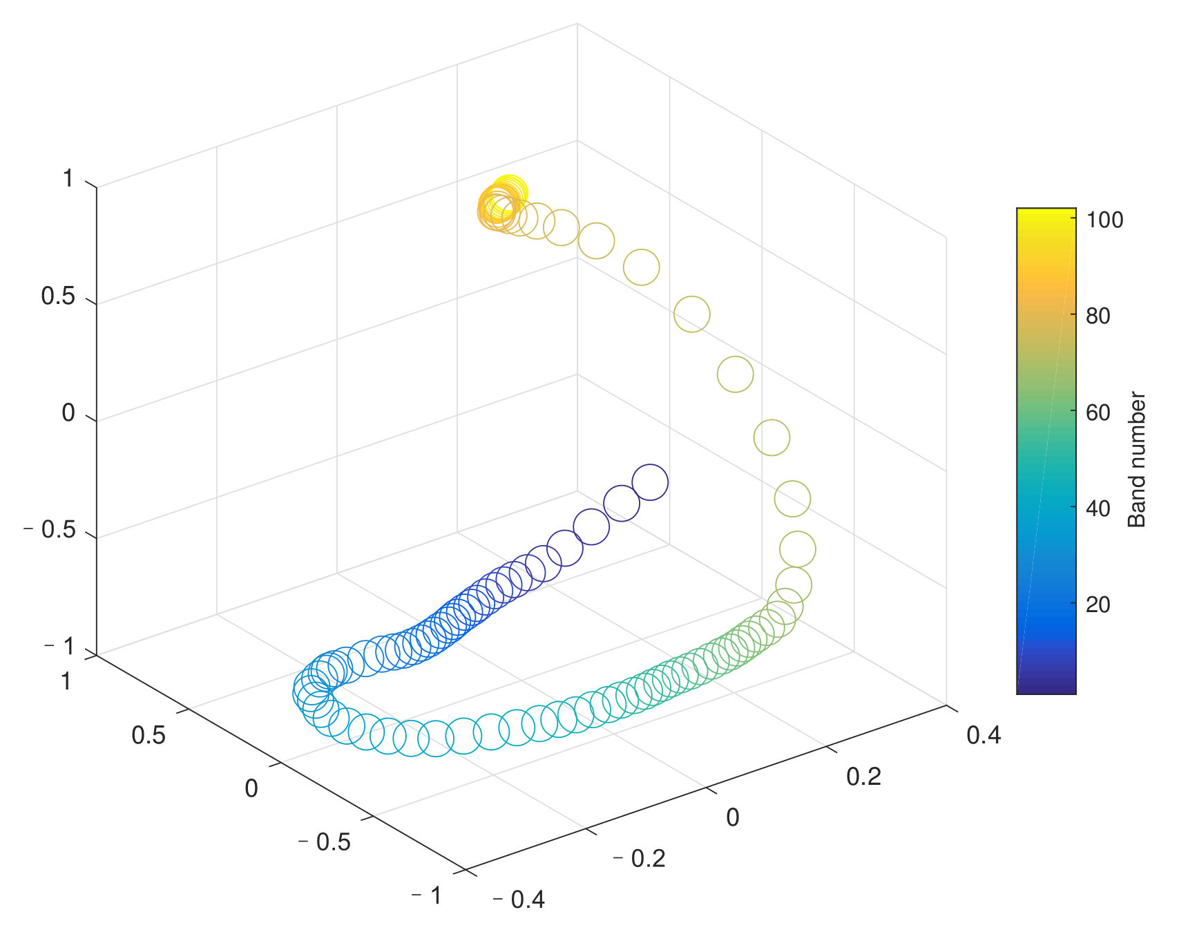
In HSIs, adjacent bands are most probably located in the same cluster [18], which is rational because each band has a stronger correlation with the adjacent bands within a certain range and a lower correlation with farther bands [18,19]. Figure 2 illustrates the correlation of all the bands on the Pavia Centre dataset projected to a three-dimensional space. Figure 2 shows that all the bands are arranged in order and form an approximately smooth curve. This further manifests the strong correlations between adjacent bands. On this basis, we propose a consensus function ILWEA by improving the consensus function LWEA used in the LWEC method [31]. As stated in Section 2.2, LWEA is a consensus function used for hierarchical agglomerative clustering that iteratively performs cluster merging by finding two clusters with the maximum similarity. However, LWEA was not developed for hyperspectral band selection. Therefore, we improved LWEA on two aspects to enhance its band selection performance. (1) LWEA performs cluster merging by finding two clusters with maximum similarity among all the obtained clusters. In the proposed ILWEA, we improved this procedure by merging two adjacent clusters with the highest similarity, which can make full use of the similarity relationship between the adjacent bands to enhance the effectiveness of the clustering results. (2) The similarity measurements of two clusters used in LWEA equally consider the similarities between data samples included in these two clusters; we improved this similarity measurement and its updating strategy by simultaneously exploiting the similarity between the nonadjacent bands as well as the important influence of the similarity of the adjacent bands included in two adjacent clusters. More precisely, in the updating strategy of the similarity between adjacent clusters in the procedure of ensemble clustering, the weights of the similarity measurements of two adjacent bands contained in two adjacent clusters, respectively, are enhanced. Thus, the importance of the similarity between adjacent bands is enforced. With these improvements, our proposed consensus function can effectively exploit both the similarity between the nonadjacent bands and the similarity between the adjacent bands, which is more in line with the characteristics of hyperspectral data.

Specifically, ILWEA first treats each band as an initial cluster, from which we can obtain the initial cluster set $C^{\left(0\right)}=\left\{G_1^{\left(0\right)},G_2^{\left(0\right)},\cdots ,G_N^{\left(0\right)}\right\}$ with $G_i^{\left(0\right)}=\left\{{\mathbf{b}}_i\right\}$, where ${\mathbf{b}}_i={\mathbf{B}}_{i:}$ and $i=1,2,\cdots ,N$. Next, by referring to [31], the initial similarity vector ${\mathbf{x}}^{\left(0\right)}$ is constructed on the basis of the LWCA matrix $\mathbf{W}$, which is expressed as

$${\mathbf{x}}^{\left(0\right)}=\left(x_1^{\left(0\right)},x_2^{\left(0\right)},\cdots ,x_i^{\left(0\right)},\cdots ,x_{N-1}^{\left(0\right)}\right),$$

(10)

with

$$x_i^{\left(0\right)}={\mathbf{w}}_{i(i+1)},$$

(11)

where ${\mathbf{w}}_{i(i+1)}$ denotes the similarity measurement between the adjacent bands ${\mathbf{b}}_i$ and ${\mathbf{b}}_{(i+1)}$.

After constructing the initial similarity vector and initial clusters, the cluster merging process is implemented iteratively. In each step of the cluster merging, instead of performing cluster merging by finding two clusters with maximum similarity, as is done in LWEA, two adjacent clusters with the highest similarity are merged into a larger cluster so that the obtained ensemble clustering results better satisfy the characteristics of HSIs. More precisely, given that $G_i^{\left(j\right)}=\left\{{\mathbf{b}}_{\alpha },{\mathbf{b}}_{\alpha +1},\cdots ,{\mathbf{b}}_{\delta }\right\}$ and $G_{i+1}^{\left(j\right)}=\left\{{\mathbf{b}}_{\delta +1},{\mathbf{b}}_{\delta +2},\cdots ,{\mathbf{b}}_{\eta }\right\}$ are two adjacent clusters in the j-th iteration, if the similarity measurement $x_i^{\left(j\right)}$ between $G_i^{\left(j\right)}$ and $G_{i+1}^{\left(j\right)}$ is highest among all the adjacent clusters, $G_i^{\left(j\right)}$ and $G_{i+1}^{\left(j\right)}$ are combined into a new cluster $G_i^{(j+1)}$. Formally, this can be expressed as

$$G_i^{(j+1)}=E\left(G_i^{\left(j\right)},G_{i+1}^{\left(j\right)}\right),$$

(12)

with

$$i=min\left(\left\{v|v\in \left\{1,2,...,(N-j-1)\right\}\wedge \forall s\in \left\{1,2,...,(N-j-1)\right\}:x_s^{\left(j\right)}\le x_v^{\left(j\right)}\right\}\right),$$

(13)

where the function $min\left(H\right)$ is used to calculate the minimum element of set H, and $E(·)$ represents the merging operation of two clusters. Accordingly, the set of clusters obtained in the $(j+1)$-th step is represented as follows:

$$C^{(j+1)}=\left\{G_1^{(j+1)},\cdots ,G_{\left|C^{(j+1)}\right|}^{(j+1)}\right\},$$

(14)

where $\left|C^{(j+1)}\right|$ denotes the number of clusters in $C^{(j+1)}$.

To prepare for the next iteration, ILWEA will update the similarity vector on the basis of the new cluster set obtained in each iteration. Here, based on updating the LWCA matrix in [31], we further introduce the similarity measurement of adjacent bands into the updating strategy of the similarity vector to enhance the importance of the similarity between adjacent bands. More formally, the updating vector of the $(j+1)$-th step is calculated as follows:

$${\mathbf{x}}^{(j+1)}=\left(x_1^{(j+1)},x_2^{(j+1)},\cdots ,x_i^{(j+1)},\cdots ,x_{\left|C^{(j+1)}\right|-1}^{(j+1)}\right),$$

(15)

with

$$x_i^{(j+1)}=\frac{1}{2}\left(\frac{1}{\left|G_i^{(j+1)}\right|·\left|G_{i+1}^{(j+1)}\right|-1}\left(\sum _{{\mathbf{b}}_m\in G_i^{(j+1)},{\mathbf{b}}_n\in G_{i+1}^{(j+1)}}{\mathbf{w}}_{mn}-{\mathbf{w}}_{\delta (\delta +1)}\right)\right)+\frac{1}{2}{\mathbf{w}}_{\delta (\delta +1)},$$

(16)

where $\left|G_i^{(j+1)}\right|$ denotes the number of bands in the cluster $G_i^{(j+1)}$. In Equation (16), the first term denotes the average value of the similarity of nonadjacent bands between the cluster $G_i^{(j+1)}=\left\{{\mathbf{b}}_{\alpha },{\mathbf{b}}_{\alpha +1},\cdots ,{\mathbf{b}}_{\delta }\right\}$ and $G_{i+1}^{(j+1)}=\left\{{\mathbf{b}}_{\delta +1},{\mathbf{b}}_{\delta +2},\cdots ,{\mathbf{b}}_{\eta }\right\}$. The second term is the similarity of the adjacent bands $b_{\delta }$ and $b_{\delta +1}$, which correspond to the last band of $G_i^{(j+1)}$ and the first band of $G_{i+1}^{(j+1)}$, respectively. Equation (16) is advantageous because we simultaneously consider the similarity between nonadjacent bands and the important influence of the similarity of adjacent bands between two adjacent clusters, which is more favorable for generating effective consensus partition.

Finally, the final consensus clustering ${\pi }^{*}=\left\{G_1^{*},G_2^{*},\cdots ,G_l^{*},\cdots ,G_L^{*}\right\}$ can be obtained when the number of clusters is equal to L, where L denotes the number of selected bands. To further illustrate the procedure of how to merge clusters in each iteration, we take an example below (see Figure 3a,b. Given $C^{\left(0\right)}=\left\{G_1^{\left(0\right)},G_2^{\left(0\right)},\cdots ,G_5^{\left(0\right)}\right\}=\left\{\left\{{\mathbf{b}}_1\right\},\left\{{\mathbf{b}}_2\right\},\left\{{\mathbf{b}}_3\right\},\left\{{\mathbf{b}}_4\right\},\left\{{\mathbf{b}}_5\right\}\right\}$, and with $x^{\left(0\right)}=\left(0.65,0.61,0.62,0.63\right)$ obtained by Equation (10), we can find that the similarity between clusters $G_1^{\left(0\right)}$ and $G_2^{\left(0\right)}$ is the highest among those of all the adjacent clusters. Thus, according to Equation (12), $G_1^{\left(0\right)}$ and $G_2^{\left(0\right)}$ are merged into a new cluster $G_1^{\left(1\right)}=\left\{{\mathbf{b}}_1,{\mathbf{b}}_2\right\}$. Accordingly, $C^{\left(1\right)}=\left\{\left\{{\mathbf{b}}_1,{\mathbf{b}}_2\right\},\left\{{\mathbf{b}}_3\right\},\left\{{\mathbf{b}}_4\right\},\left\{{\mathbf{b}}_5\right\}\right\}$ is obtained.

2.3.2. Manifold Ranking for Representative Band Selection

Most conventional clustering-based methods select representative bands from the obtained clusters using some kinds of criteria, such as information divergence [17], band noise estimation [19], and band distance from the centroid [28]. However, these algorithms are unfavorable for selecting representative bands because the most discriminative bands in each cluster may not be discriminative as regards all bands [18]. To tackle this issue, we improve the manifold ranking method [21] to rank all bands while ensuring that only one band is selected from each cluster according to the rank information.

Specifically, let $\mathbf{y}=\left(y_1,y_2,\cdots ,y_n,\cdots ,y_N\right)$ represent an indicating vector, with $y_n=1$ denoting that the corresponding band ${\mathbf{b}}_n$ is included in the representative band set $\mathsf{\Phi }$. To indicate whether the cluster $G_l^{*}$ has been used in selecting the representative band, a vector $\mathbf{a}=\left(a_1,a_2,\cdots ,a_n,\cdots ,a_N\right)$ is employed. First, we select the band ${\mathbf{b}}_i$ with the largest variance from all bands and put ${\mathbf{b}}_i$ into the initial representative band set $\mathsf{\Phi }$. Then, we set the value of ${\mathbf{y}}^{\left(0\right)}=(y_1^{\left(0\right)},y_2^{\left(0\right)},\cdots ,y_n^{\left(0\right)},\cdots ,y_N^{\left(0\right)})$ as

$$y_n^{\left(0\right)}=\left\{\begin{array}{cc}1,\hfill & \mathrm{if}n=i\hfill \\ 0,\hfill & \mathrm{otherwise}\hfill \end{array}.\right.$$

(17)

Meanwhile, we set ${\mathbf{a}}^{\left(0\right)}=(a_1^{\left(0\right)},a_2^{\left(0\right)},\cdots ,a_n^{\left(0\right)},\cdots ,a_N^{\left(0\right)})$ where $a_n^{\left(0\right)}$, for $n=1,2,\cdots ,N$, is set to 1 if ${\mathbf{b}}_n$ belongs to the same cluster with ${\mathbf{b}}_i$, and 0 otherwise. This can be formalized as

$$a_n^{\left(0\right)}=\left\{\begin{array}{cc}1,\hfill & \mathrm{if}Gl{s}^{*}\left(b_i\right)=Gl{s}^{*}\left(b_n\right)\hfill \\ 0,\hfill & \mathrm{otherwise}\hfill \end{array},\right.$$

(18)

where $Gl{s}^{*}\left({\mathbf{b}}_i\right)\in {\pi }^{*}$ denotes the cluster to which band ${\mathbf{b}}_i$ belongs.

Next, to select the remaining representative bands, we iteratively perform the following procedures: (1) Compute the ranking score vector $\mathbf{q}\in {\mathbb{R}}^N$ according to the sorting function that is expressed as [37]

$$\mathbf{q}={(\mathbf{D}-\alpha \mathbf{W})}^{-1}\mathbf{y},$$

(19)

with

$$\mathbf{D}=diag\left\{d_{11},d_{22},\cdots ,d_{nn},\cdots ,d_{NN}\right\},$$

(20)

where $\mathbf{W}$ is the LWCA matrix, and $d_{nn}={\sum }_j{\mathbf{w}}_{nj}$; $\alpha$ denotes a balance parameter. (2) Select a representative band ${\mathbf{b}}_s={\mathbf{B}}_{s:}$ where the index s is determined by

$$s=min\left(\left\{n|(n\in \left\{1,2,...,N\right\}\wedge a_n^{(k-1)}\ne 1)\wedge (\forall t\in \left\{1,2,...,N\right\}\wedge a_t^{(k-1)}\ne 1):q_n\le q_t\right\}\right).$$

(21)

(3) Put the selected band ${\mathbf{b}}_s$ into the representative band set $\mathsf{\Phi }$. (4) Update ${\mathbf{y}}^{\left(k\right)}$ by

$$y_n^{\left(k\right)}=\left\{\begin{array}{cc}1,\hfill & \mathrm{if}n=s\hfill \\ y_n^{(k-1)},\hfill & \mathrm{otherwise}\hfill \end{array},\right.$$

(22)

and update ${\mathbf{a}}^{\left(k\right)}$ by

$$a_n^{\left(k\right)}=\left\{\begin{array}{cc}1,\hfill & \mathrm{if}Gl{s}^{*}\left(b_s\right)=Gl{s}^{*}\left(b_n\right)\hfill \\ a_n^{(k-1)},\hfill & \mathrm{otherwise}\hfill \end{array}.\right.$$

(23)

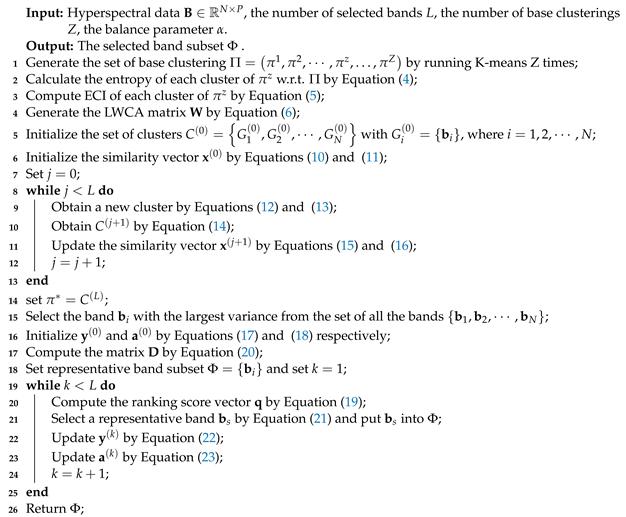
Finally, the algorithm is stopped when the number of bands included in $\mathsf{\Phi }$ is equal to L. As a result, the bands contained in $\mathsf{\Phi }$ are regarded as the selected representative bands. On the basis of the above analysis, the pseudocode of our proposed CGEC algorithm is outlined in Algorithm 1.

Algorithm 1: CGEC Algorithm

3. Result

3.1. Datasets

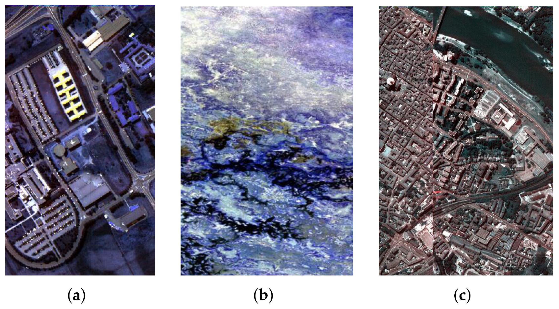
In our experiments, three benchmark datasets respectively listed in

Table 1. Information on the three real datasets used in our experiments.

Dataset Names	Pixels	Spatial Resolutions	Classes	Bands
Pavia University	610 × 340	1.3 m/pixel	9	103
Botswana	1476 × 256	30 m/pixel	14	145
Pavia Centre	1096 × 715	1.3 m/pixel	9	102

and displayed in Figure 4 were chosen to test the performance of the proposed approach according to the classification accuracy criteria.

1. Pavia University dataset: The Pavia University dataset is part of the hyperspectral data taken from the image of the Italian city of Pavia in 2002 by the Reflective Optics System Imaging Spectrometer (ROSIS) sensor. This image has 610 × 340 pixels and 115 bands with wavelengths ranging from 0.43 $\mathsf{\mu }$m to 0.86 $\mathsf{\mu }$m, and its spatial resolution is 1.3 m. In our experiments, 12 bands were eliminated because of the influence of noise, and the image made up of the remaining 103 spectral bands was used. There are 9 classes in this image.

2. Botswana dataset: The Botswana dataset was acquired by the NASA EO-1 satellite over the Okavango Delta, Botswana, in 2001. The original Botswana image has 242 bands covering wavelengths from 0.4 µm to 2.5 µm, and its spatial resolution is 30 m. After some uncalibrated and noisy bands were removed, the remaining 145 spectral bands were used in this study. The adopted image has 1476 × 256 pixels and 14 classes.

3. Pavia Centre dataset: The Pavia Centre dataset was obtained by the ROSIS sensor during a flight campaign over Pavia in northern Italy. Thus, it has the same spectral and spatial resolution as those of the first dataset. In our experiments, the noisy bands were removed, and the remaining 102 bands were used. This image has 1096 × 715 pixels that belong to nine different classes.

3.2. Comparison Methods

Seven representative band selection methods, briefly introduced in this section, were used as baselines to verify the effectiveness of the proposed methods.

1. E-FDPC [15]: Enhanced fast-density-peak-based clustering (E-FDPC) is a clustering-based method that improved a fast density peak-based clustering [38] algorithm by weighting the local density and the distance within the cluster. In addition, it adopts an exponential-based learning rule to control the number of selected bands of HSIs.

2. ASPS [19]: ASPS is also a clustering-based method for band selection. It first divides the HSI cube into several subcubes by maximizing the ratio of the intercluster distance to the intracluster distance, and then estimates the band noise in each subcube. Thereafter, the band containing the minimum noise in each cluster is selected as the target band.

3. WaLuDi [17]: This method uses the hierarchical clustering technique to select representative bands. To measure the dissimilarity among the bands, the Kullback–Leibler divergence is employed in the clustering procedure.

4. NC-OC-IE [18]: It is a clustering-based method that adopts an optimal clustering framework (OCF) to search for the optimal clustering structure on HSIs. First, an objective function based on a normalized cut criterion is designed. Then, the best band partition is obtained using OCF. Next, the importance of all the bands is evaluated using the information entropy-based criterion. Finally, the target bands are found by selecting the highest-ranked band in each cluster.

5. MVPCA [16]: MVPCA is a ranking-based method that evaluates the band prioritization by constructing a data-sample covariance matrix. Then, all bands are ranked according to the matrix. The band subset can be obtained by selecting the top-rank bands.

6. LWEA [31]: LWEA is an ensemble clustering method based on hierarchical agglomerative clustering, which utilizes a similarity matrix as input and iteratively performs cluster merging by finding two clusters with the maximum similarity.

7. DSC [29]: DSC is a clustering-based band selection approach that exploits a convolutional autoencoder and deep subspace clustering to obtain the clustering results. Then, the final band subset can be obtained by selecting the band closest to its cluster center in each cluster.

3.3. Experimental Setup

1. Classification setting

Support vector machine (SVM) [39] and K-nearest neighbor (KNN) [40] were used to test the classification accuracy of different band selection methods. In the experiments, we randomly selected 20% of the samples as the training set, and the rest of the samples were used as the test set. Each method was run 10 times, and the average performance was reported. To test the influence of different band numbers on overall accuracy, we conducted experiments in the range of 5–50 bands. In addition, by referring to [31], 10 base clusterings were randomly produced by running the K-means algorithm with different numbers of clusters L. The range of L is from 2 to $\sqrt{N}$, where N denotes the number of bands in HSIs. The balance parameter $\alpha$ in Equation (19) is set to 0.99 according to [37].

2. Accuracy measures

Three accuracy criteria are used to analyze the accuracy of the classified pixels. These criteria are overall accuracy (OA), average overall accuracy (AOA), and Kappa coefficient (Kappa).

3.4. Experimental Results

To test the performance of the proposed approach, two classifiers were adopted to analyze three hyperspectral datasets. The average performance comparison of all the methods for different numbers of bands (the range of 5–50) is reported in

Table 2. Performance comparison on the three datasets, where larger values indicates better performance; the values in red bold and blue italic fonts denote the best and second-best results, respectively. CGEC is our proposed approach.

Dataset	Classifier	CGEC	LWEA [31]	E-FDPC [15]	NC-OC-IE [18]	ASPS [19]	WaLudi [17]	MVPCA [16]	DSC [29]
Pavia University	SVM(AOA)	90.09	89.86	85.21	89.58	88.70	88.17	77.22	89.64
	SVM(KAPPA)	0.8670	0.8640	0.7998	0.8600	0.8479	0.8412	0.6660	0.8611
	KNN(AOA)	84.22	83.86	82.15	84.02	83.83	82.33	72.53	84.15
	KNN(KAPPA)	0.7836	0.7794	0.7554	0.7809	0.7789	0.7574	0.6219	0.7827
Botswana	SVM(AOA)	90.43	90.13	74.10	89.87	89.03	85.77	78.44	88.53
	SVM(KAPPA)	0.8961	0.8932	0.7194	0.8902	0.8811	0.8458	0.7662	0.8758
	KNN(AOA)	86.42	85.19	63.52	85.62	83.39	80.82	72.91	82.67
	KNN(KAPPA)	0.8527	0.8396	0.6052	0.8442	0.8201	0.7922	0.7065	0.8109
Pavia Centre	SVM(AOA)	98.11	95.27	91.28	87.91	88.55	88.75	73.77	90.60
	SVM(KAPPA)	0.9731	0.9446	0.9037	0.8715	0.8767	0.8796	0.7090	0.8980
	KNN(AOA)	97.14	96.96	96.95	97.04	96.80	96.97	87.92	97.05
	KNN(KAPPA)	0.9596	0.9570	0.9569	0.9589	0.9547	0.9572	0.8249	0.9591

, where the classification performance of the SVM and KNN classifiers is indicated by the AOA and Kappa. Each row represents the classification accuracy of a specified classifier for the target dataset using the bands given by different methods. The values in red bold and blue italic fonts denote the best and second-best results, respectively. Table 2 shows that the superiority of CGEC is evident in comparison with the other band selection approaches. Particularly, when using an SVM classifier on the Pavia Centre dataset, our method can achieve an improvement of 2.84% and 2.85% in AOA and Kappa, respectively, compared with LWEA. LWEA had the second-best performance when using an SVM classifier on the three datasets. DSC obtained the second-best results when using a KNN classifier on the Pavia University and Pavia Centire datasets. For the Botswana dataset, the second best is NC-OC-IE.

To further demonstrate the performance of all the methods, the classification results for each class on the three datasets using 30 selected bands are listed in

Table 3. The classification accuracy of each class for the Pavia University dataset, where larger values indicate better performance; the values in red bold and blue italic fonts denote the best and second-best results, respectively. CGEC is our proposed approach.

Class Name	CGEC	LWEA [31]	E-FDPC [15]	NC-OC-IE [18]	ASPS [19]	WaLudi [17]	MVPCA [16]	DSC [29]
Asphalt	91.61	91.51	88.61	91.42	91.31	89.24	86.11	91.55
Meadows	97.13	96.79	96.62	96.83	97.15	94.95	98.01	97.05
Gravel	71.90	70.98	53.75	71.27	69.66	68.95	61.36	69.56
Trees	94.12	93.72	87.49	93.97	93.93	92.17	92.06	93.82
Metal sheets	99.73	99.54	99.68	99.70	99.69	99.67	99.59	99.62
Bare Soil	80.56	80.45	53.39	77.33	75.93	71.87	50.97	80.14
Bitumen	82.36	82.49	72.74	82.08	81.90	80.00	65.66	80.56
Bricks	86.96	86.88	83.15	87.64	87.86	83.87	75.38	86.79
Shadows	99.72	99.80	93.79	99.34	98.93	99.78	96.07	99.87

,

Table 4. The classification accuracy of each class for the Botswana dataset, where larger values indicate better performance; the values in red bold and blue italic fonts denote the best and second-best results, respectively. CGEC is our proposed approach.

Class Name	CGEC	LWEA [31]	E-FDPC [15]	NC-OC-IE [18]	ASPS [19]	WaLudi [17]	MVPCA [16]	DSC [29]
Water	100.00	99.86	92.13	99.58	99.61	99.88	98.70	96.90
Hippo grass	97.78	96.04	73.21	94.94	96.67	96.90	96.91	89.26
Floodplain grasses 1	97.71	97.61	87.51	96.07	95.47	96.32	84.43	95.57
Floodplain grasses 2	97.62	97.15	77.68	94.88	93.78	95.87	91.51	93.60
Reeds 1	86.23	86.13	68.51	80.65	83.49	84.14	78.84	84.28
Riparian	80.37	78.72	57.26	79.54	77.53	72.37	68.93	75.12
Firescar 2	98.70	96.78	92.22	98.12	98.07	98.08	91.45	88.84
Island interior	98.15	98.27	76.11	97.96	96.36	94.26	91.61	97.47
Acacia woodlands	91.79	92.71	77.89	91.00	86.81	87.49	88.45	88.01
Acacia shrublands	90.00	89.24	80.00	90.05	88.64	88.03	86.11	85.61
Acacia grasslands	92.01	93.49	89.26	93.32	92.58	91.51	86.72	91.96
Short mopane	92.27	92.90	68.14	94.07	92.27	92.76	76.83	83.86
Mixed mopane	92.80	92.52	65.89	90.75	89.77	90.05	83.50	79.58
Exposed soils	97.37	97.89	83.29	97.24	95.92	93.95	64.21	94.87

and

Table 5. The classification accuracy of each class for the Pavia Centre dataset, where larger values indicate better performance; the values in red bold and blue italic fonts denote the best and second-best results, respectively. CGEC is our proposed approach.

Class Name	CGEC	LWEA [31]	E-FDPC [15]	NC-OC-IE [18]	ASPS [19]	WaLudi [17]	MVPCA [16]	DSC [29]
Water	100.00	99.98	99.97	99.95	99.98	99.93	99.99	99.99
Trees	96.75	95.40	95.67	96.89	95.75	95.72	95.58	96.44
Asphalt	92.26	89.54	90.38	92.20	90.27	89.36	81.77	92.44
Bricks	87.50	85.70	79.05	87.31	83.48	87.42	66.84	87.15
Bitumen	96.91	96.26	94.30	96.87	95.73	96.30	75.08	96.69
Tiles	96.13	95.67	96.02	95.35	96.21	96.23	88.36	96.47
Shadows	93.59	93.16	92.16	93.31	93.53	93.44	86.83	93.12
Meadows	99.56	99.46	99.60	99.64	99.63	99.53	97.91	99.59
Bare soil	99.86	99.80	98.45	99.68	99.39	99.50	91.95	99.40

. The values in red bold and blue italic fonts denote the best and second-best results, respectively. Clearly, our proposed method performs best or second best at most classes on three datasets. Some methods are slightly unstable. For example, the performance of LWEA is better on the Botswana dataset, but slightly worse on the other datasets. DSC performs better on the Botswana dataset than on the other datasets. This shows the effectiveness and stability of our method on the three datasets. In addition, Figure 5, Figure 6 and Figure 7 illustrate the OA values of all eight methods on the three datasets when using the SVM and KNN classifiers, respectively. More detailed analyses are given as follows.

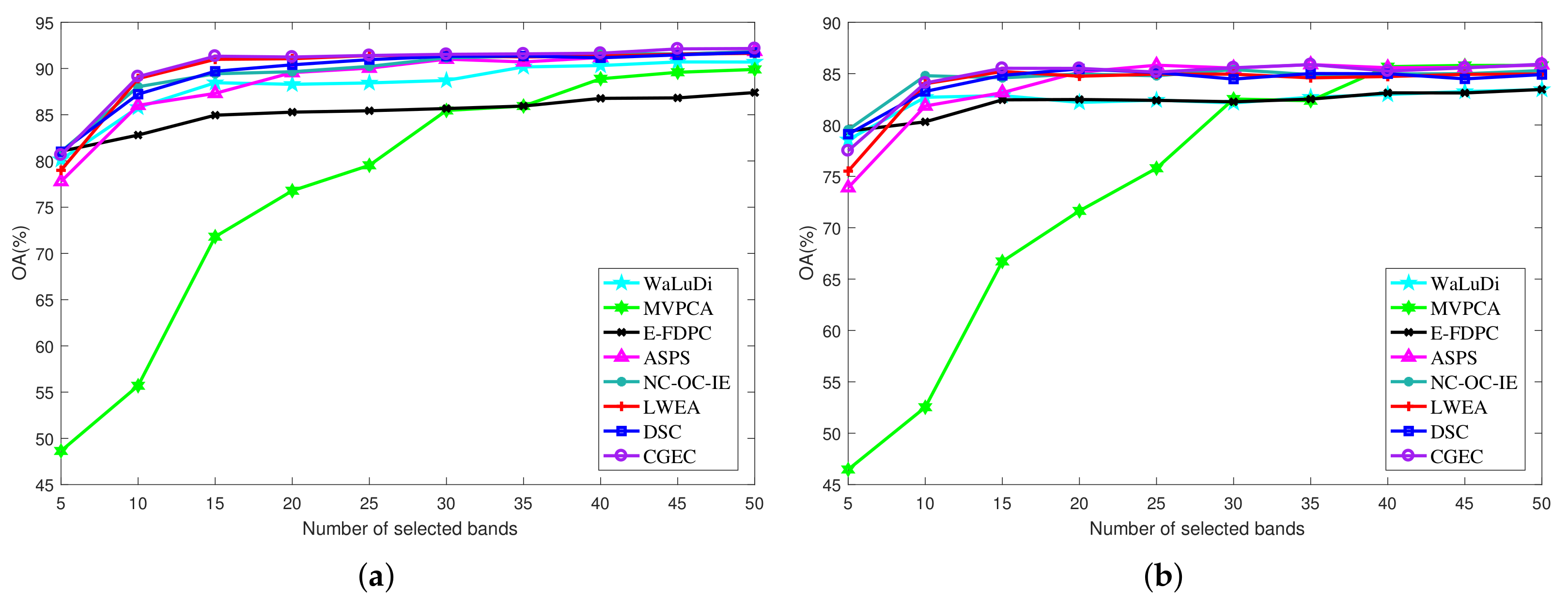
Pavia University dataset. For this dataset, Figure 5a,b indicate the OA results of the SVM and KNN classifiers using bands given by all the methods. The range of the number of bands selected is from 5 to 50. Figure 5a clearly shows that when using an SVM classifier, the performance of CGEC is better than those of the other algorithms at most of the selected bands. More specifically, when the numbers of selected bands are 10, 15, and 25, our method surpasses the other methods and achieves a satisfactory classification accuracy. It is worth noting that the data redundancy is obviously reduced via the band selection process, and more than 90% of the redundant bands in the original dataset are removed. When the number of the selected bands exceeds 30, our method also performs best, and the OA values of LWEA, DSC, ASPS, and NC-OC-IE are close to each other. Meanwhile, these four methods outperform the other methods. In Figure 5b, when using a KNN classifier, the OA value of CGEC is better than those of the other methods when using 15, 20, 30, 35, and 50 bands. For the other bands, although our method is slightly lower than NC-OC-IE or MVPCA, it outperforms other approaches.

Botswana dataset. Similar to the Pavia University dataset, Figure 6a,b illustrate the OA results of the classification using SVM and KNN, respectively. Figure 6a shows that the OA value of the CGEC method is the highest except when the number of selected bands is 35. At 35 bands, our method achieves the second-best performance. In Figure 6b, our method shows significant superiority when the numbers of selected bands are 5, 10, 15, and 25. At the same time, the OA values of the CGEC, LWEA, ASPS, WaLuDi, and NC-OC-IE approaches are close to each other at the other bands, which outperform the other methods. In general, the effectiveness of our method is verified.

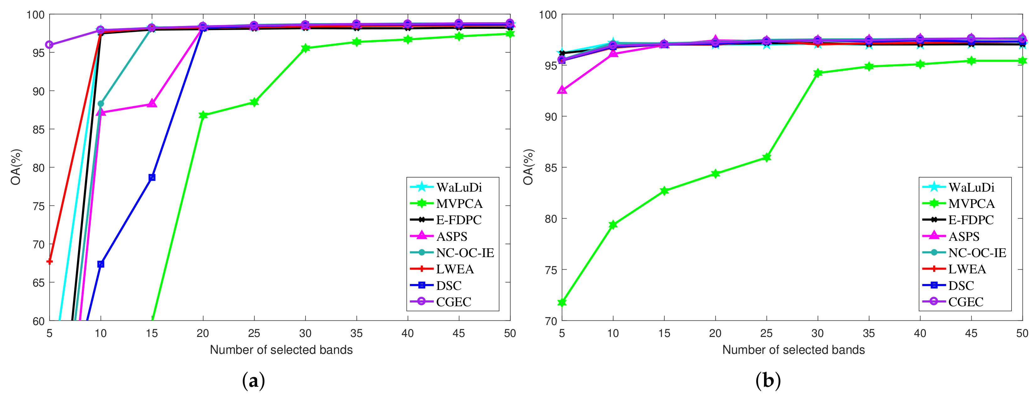
Pavia Centre dataset. For this dataset, the advantage of our approach is more apparent when using the SVM classifier, as shown in Figure 7a. When the number of selected bands is 5, our method is significantly better than the other methods. Remarkably, the proposed method achieves a satisfactory result with only 5% of the bands from the dataset. When the number of selected bands exceeds 5, our method also performs very well. In Figure 7b, when KNN is utilized, the difference in the OA values is not obvious, and all the methods attain satisfying results, except for MVPCA.

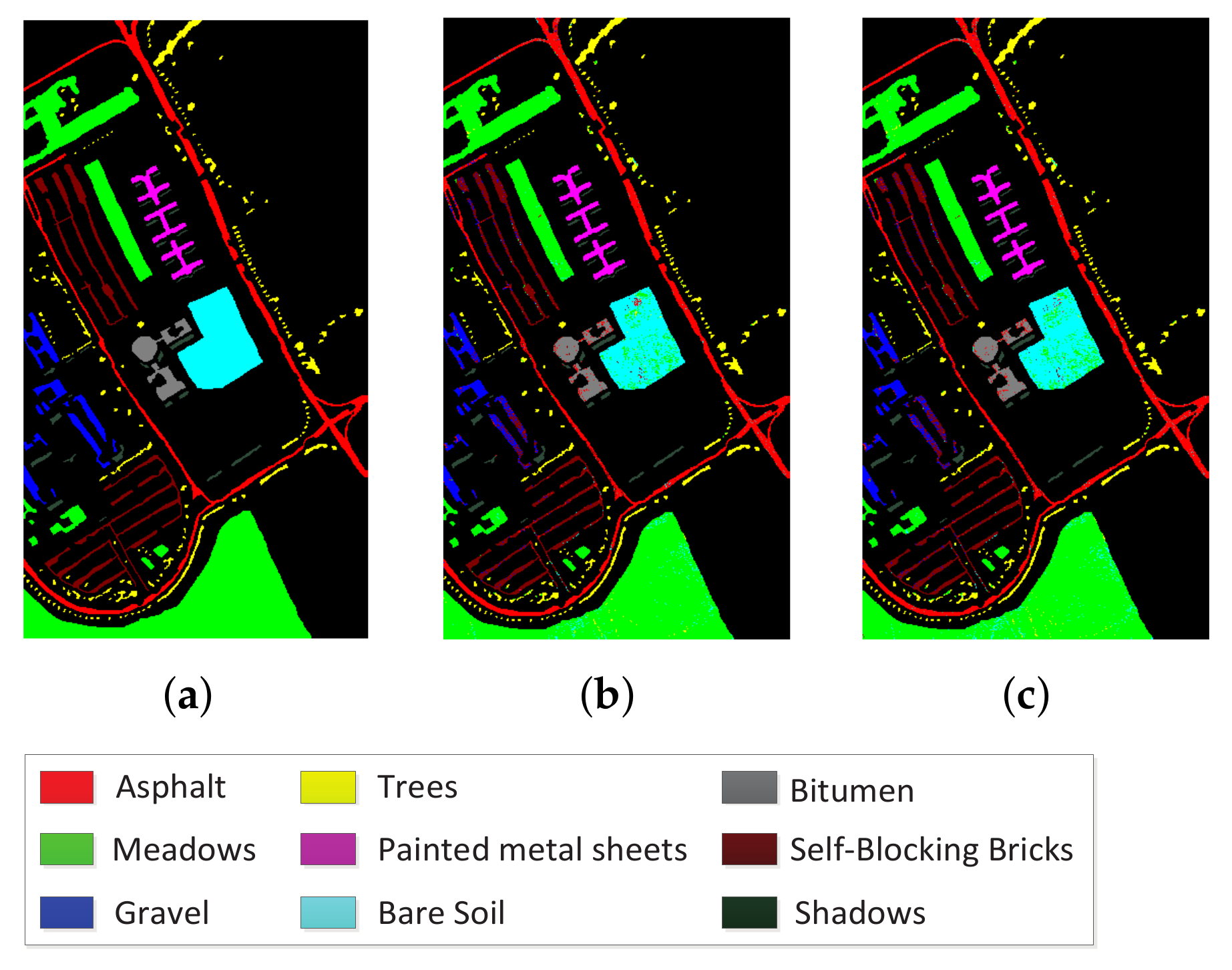
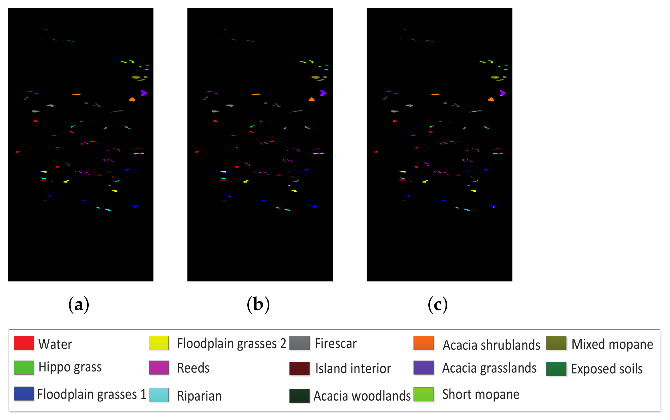
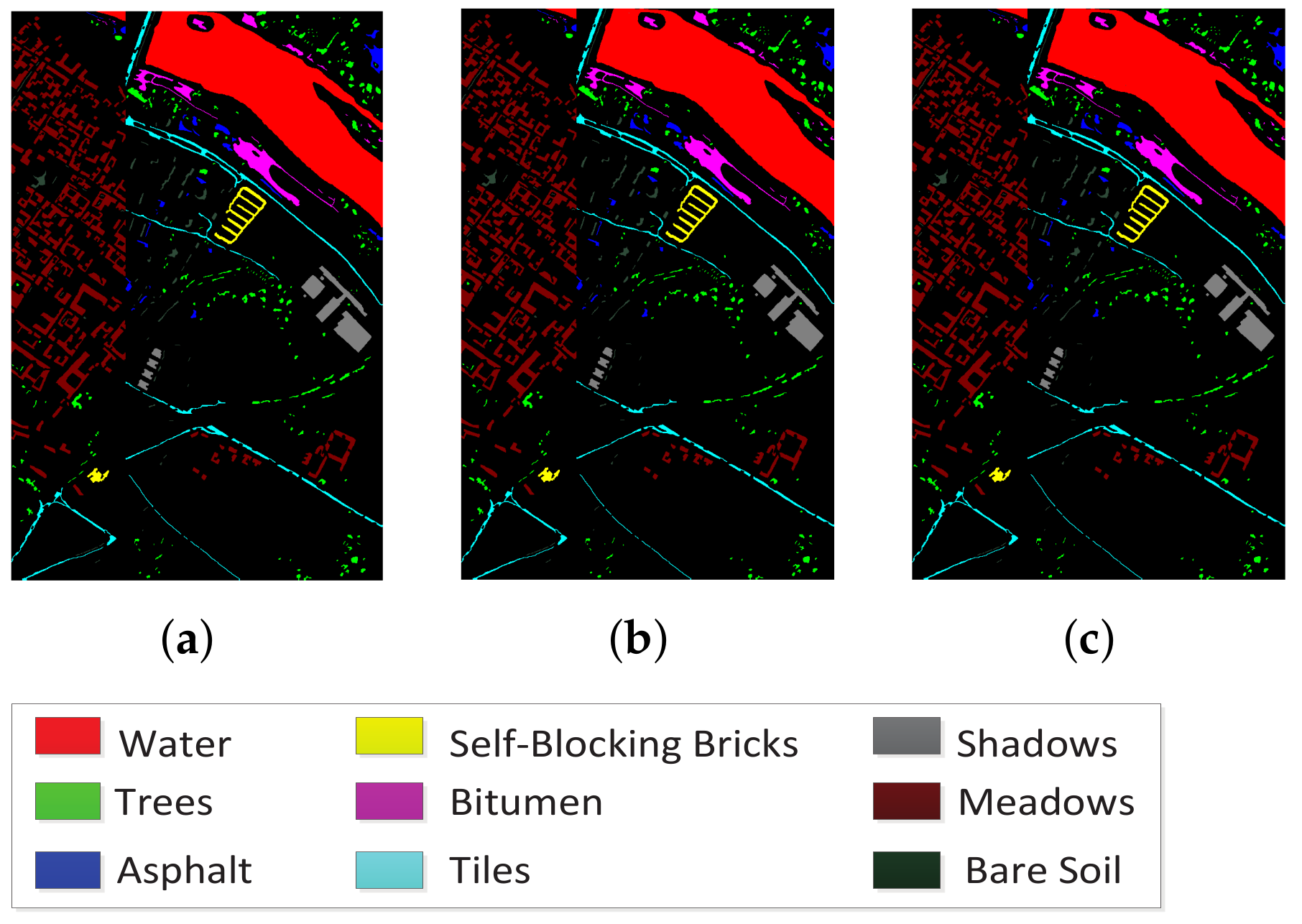
In addition, Figure 8, Figure 9 and Figure 10 compare classification maps and ground truth information using 30 selected bands. These classification maps indicate that our method can provide satisfactory results on condition that 79% of the bands from the Botswana dataset, as well as 70% of the bands from the Pavia Center and Pavia University datasets are removed. Therefore, our method can reduce lots of redundant information while maintaining good classification accuracy.

4. Discussion

Band selection is one of the important dimensionality reduction techniques for hyperspectral classification. Aiming to select more representative bands from HSIs by enhancing the accuracy of clustering, in this paper, LWEA, a recently proposed ensemble clustering method, was improved to tackle the band selection problem. The original LWEA can obtain better clustering performance by implementing aggregation clustering. However, it performs cluster merging by only finding two clusters with maximum similarity among all the obtained clusters without considering the characteristics of HSIs. Moreover, the similarity measurements between two clusters used in LWEA equally consider the similarities among data samples included in these two clusters, which may not meet the needs of band selection. Experimental results have demonstrated these issues limit the algorithm performance for band selection. Based on the assumption that adjacent bands in HSIs have a high correlation, and thus they are most probably located in the same cluster, in this paper, we proposed CGEC by improving the cluster merging procedure of LWEA, which can make full use of the similarity relationship between the adjacent bands to generate effective ensemble clustering results. Moreover, based on the clustering results provided by CGEC, our modified manifold ranking method can contribute to selecting more representative bands. To the best of our knowledge, this is the first time that ensemble clustering has been applied to the band selection of HSIs. The experimental results presented in the previous section demonstrate that ensemble clustering is more effective for band selection compared with the single clustering-based band selection methods and LWEA. In addition, exploiting the similarity relationship between adjacent bands in the design of consensus function can effectively enhance the performance of ensemble clustering for band selection.

According to the experimental results, the clustering-based methods achieved better performance than the ranking-based method (i.e., MVPCA). This is because the selected bands of MVPCA have higher redundancy. This finding is consistent with that of a previous study [41]. In contrast, the clustering-based methods can remove the redundant bands by selecting a representative band from each cluster. Compared with representative clustering-based methods (i.e., E-FDPC, NC-OC-IE, ASPS, WaLudi, DSC, and LWEA), our proposed CGEC has remarkable performance due to the use of ensemble clustering with the guidance of band correlation property of HSIs. A clear explanation lies in the fact that the cluster results given by CGEC meet the need of band selection, which helps to select more representative bands. Thus, we believe that our method can provide more effective clustering results on the HSI in which each band has a stronger correlation with the adjacent bands.

The experimental results also demonstrate that the number of selected bands has a significant influence on classification performance. For example, a general phenomenon for all the methods lies in the fact that, as shown in Figure 5, Figure 6 and Figure 7, the OA values rise rapidly with the increase of the number of bands, but when a certain number of bands are reached, the increase is very slight or even decreased. In accordance with our results, a previous study [42] has demonstrated that the best performances do not always exist in the band subset with the most bands. The reason is that more bands bring more redundancies. Consequently, selecting more bands does not mean that better classification accuracy can be obtained, while a reasonable number of bands will achieve the best performance.

We have to point out that our study neglects noise interference in HSIs. Thus, the proposed CGEC may choose the noisy bands, which will degrade the classification performance. In addition, base clustering in our method is carried out on the original high-dimensional data, so the quality of base clustering is limited, which will affect the effectiveness of the ensemble clustering result. In future studies, we will explore the strategy of generating more effective base clustering based on representation learning to further improve the band selection performance of ensemble clustering.

5. Conclusions

In this paper, we proposed a correlation-guided ensemble clustering approach for hyperspectral band selection. By adopting ensemble clustering, a more accurate band partition can be obtained compared with the single clustering methods. With the help of a proposed consensus function that is designed based on the assumption that adjacent bands are most probably located in the same cluster, the clustering results of the proposed method more satisfy the needs of band selection. In addition, our proposed approach employs an improved manifold ranking algorithm to select a band subset with better representativeness from the final band partition. A variety of experiments on three real hyperspectral datasets indicate that the effectiveness of the proposed method is superior compared with other competitors. For the sake of clarity, the main conclusions of this paper are as follows.

An ensemble clustering-based approach is proposed to select representative bands for hyperspectral classification. To the best of our knowledge, this is the first time that ensemble clustering has been applied to the band selection of HSIs. The proposed approach consists of two stages, i.e., ensemble clustering and manifold ranking. The ensemble clustering stage is designed to improve the effectiveness of clustering, whereas the manifold ranking stage is exploited to select a representative band from each cluster. Consequently, the chosen band subset has good distinguishability and high representativeness for classification tasks.

In addition, we proposed a novel consensus function used for generating consensus clustering results via agglomerative clustering. By utilizing the fact that adjacent bands have high probability located in the same cluster, the proposed consensus function can simultaneously exploit the problem-independent information and the power of ensemble clustering, so that the obtained results of ensemble clustering better satisfy the needs of band selection.

To verify the effectiveness of our proposed method, we conducted extensive experiments on three real HSI datasets. The experimental results of our method were compared with those of seven representative methods, which demonstrates the superiority of our proposed method.

References

1. Gomez, C.; White, J.C.; Wulder, M.A. Optical remotely sensed time series data for land cover classification: A review. ISPRS J. Photogramm. Remote Sens. 2016, 116, 55–72. [Google Scholar] [CrossRef] [Green Version]
2. Zhao, Y.; Yuan, Y.; Wang, Q. Fast Spectral Clustering for Unsupervised Hyperspectral Image Classification. Remote Sens. 2019, 11, 399. [Google Scholar] [CrossRef] [Green Version]
3. Gao, B.; Lu, A.; Pan, Y.; Huo, L.; Gao, Y.; Li, X.; Li, S.; Chen, Z. Additional Sampling Layout Optimization Method for Environmental Quality Grade Classifications of Farmland Soil. IEEE J. Sel. Top. Appl. Earth Observ. 2017, 10, 5350–5358. [Google Scholar] [CrossRef]
4. Hosseinjani Zadeh, M.; Tangestani, M.H.; Velasco Roldan, F.; Yusta, I. Mineral Exploration and Alteration Zone Mapping Using Mixture Tuned Matched Filtering Approach on ASTER Data at the Central Part of Dehaj-Sarduiyeh Copper Belt, SE Iran. IEEE J. Sel. Top. Appl. Earth Observ. Remote Sens. 2014, 7, 284–289. [Google Scholar] [CrossRef]
5. Zarco-Tejada, P.; González-Dugo, M.; Fereres, E. Seasonal stability of chlorophyll fluorescence quantified from airborne hyperspectral imagery as an indicator of net photosynthesis in the context of precision agriculture. Remote Sens. Environ. 2016, 179, 89–103. [Google Scholar] [CrossRef]
6. Saha, S.; Mou, L.; Qiu, C.; Zhu, X.X.; Bruzzone, L. Unsupervised Deep Joint Segmentation of Multitemporal High-Resolution Images. IEEE Trans. Geosci. Remote Sens. 2020, 58, 8780–8792. [Google Scholar] [CrossRef]
7. Lv, X.; Wang, W.; Liu, H. Cluster-Wise Weighted NMF for Hyperspectral Images Unmixing with Imbalanced Data. Remote Sens. 2021, 13, 268. [Google Scholar] [CrossRef]
8. Hughes, G. On the mean accuracy of statistical pattern recognizers. IEEE Trans. Inf. Theory 1968, 14, 55–63. [Google Scholar] [CrossRef] [Green Version]
9. Sun, W.; Du, Q. Hyperspectral Band Selection: A Review. IEEE Geosci. Remote Sens. Mag. 2019, 7, 118–139. [Google Scholar] [CrossRef]
10. Bandos, T.V.; Bruzzone, L.; Camps-Valls, G. Classification of Hyperspectral Images With Regularized Linear Discriminant Analysis. IEEE Trans. Geosci. Remote Sens. 2009, 47, 862–873. [Google Scholar] [CrossRef]
11. Liu, X.; Zhang, B.; Gao, L.R.; Chen, D.M. A maximum noise fraction transform with improved noise estimation for hyperspectral images. Sci. China 2009, 52, 90–99. [Google Scholar] [CrossRef]
12. Wang, J.; Chang, C.I. Independent component analysis-based dimensionality reduction with applications in hyperspectral image analysis. IEEE Trans. Geosci. Remote Sens. 2006, 44, 1586–1600. [Google Scholar] [CrossRef]
13. Cao, X.; Tao, X.; Jiao, L. Supervised Band Selection Using Local Spatial Information for Hyperspectral Image. IEEE Geosci. Remote Sens. Lett. 2016, 13, 329–333. [Google Scholar] [CrossRef]
14. Feng, J.; Jiao, L.; Liu, F.; Sun, T.; Zhang, X. Mutual-Information-Based Semi-Supervised Hyperspectral Band Selection With High Discrimination, High Information, and Low Redundancy. IEEE Trans. Geosci. Remote Sens. 2015, 53, 2956–2969. [Google Scholar] [CrossRef]
15. Jia, S.; Tang, G.; Zhu, J.; Li, Q. A Novel Ranking-Based Clustering Approach for Hyperspectral Band Selection. IEEE Trans. Geosci. Remote Sens. 2016, 54, 88–102. [Google Scholar] [CrossRef]
16. Chang, C.I.; Du, Q.; Sun, T.L.; Althouse, M.L.G. A joint band prioritization and band-decorrelation approach to band selection for hyperspectral image classification. IEEE Trans. Geosci. Remote Sens. 1999, 37, 2631–2641. [Google Scholar] [CrossRef] [Green Version]
17. Martínez-UsÓMartinez-Uso, A.; Pla, F.; Sotoca, J.M.; García-Sevilla, P. Clustering-based hyperspectral band selection using information measures. IEEE Trans. Geosci. Remote Sens. 2008, 45, 4158–4171. [Google Scholar]
18. Qi, W.; Fahong, Z.; Xuelong, L. Optimal Clustering Framework for Hyperspectral Band Selection. IEEE Trans. Geosci. Remote Sens. 2018, 10, 5910–5922. [Google Scholar]
19. Wang, Q.; Li, Q.; Li, X. Hyperspectral Band Selection via Adaptive Subspace Partition Strategy. IEEE J. Sel. Top. Appl. Earth Observ. Remote Sens. 2019, 12, 4940–4950. [Google Scholar] [CrossRef]
20. Mou, L.; Saha, S.; Hua, Y.; Bovolo, F.; Bruzzone, L.; Zhu, X.X. Deep Reinforcement Learning for Band Selection in Hyperspectral Image Classification. IEEE Trans. Geosci. Remote Sens. 2021, 60, 1–14. [Google Scholar] [CrossRef]
21. Wang, Q.; Lin, J.; Yuan, Y. Salient Band Selection for Hyperspectral Image Classification via Manifold Ranking. IEEE Trans. Neural Net. Learn. Syst. 2017, 27, 1–11. [Google Scholar] [CrossRef] [PubMed]
22. Sun, W.; Peng, J.; Yang, G.; Du, Q. Fast and Latent Low-Rank Subspace Clustering for Hyperspectral Band Selection. IEEE Trans. Geosci. Remote Sens. 2020, 58, 3906–3915. [Google Scholar] [CrossRef]
23. Sun, W.; Li, W.; Li, J.; Lai, Y.M. Band selection using sparse nonnegative matrix factorization with the thresholded Earth’s mover distance for hyperspectral imagery classification. Earth Sci. Inform. 2015, 8, 907–918. [Google Scholar] [CrossRef]
24. Feng, Y.; Yuan, Y.; Lu, X. A non-negative low-rank representation for hyperspectral band selection. Int. J. Remote Sens. 2016, 37, 4590–4609. [Google Scholar] [CrossRef]
25. Zhai, H.; Zhang, H.; Zhang, L.; Li, P. Laplacian-Regularized Low-Rank Subspace Clustering for Hyperspectral Image Band Selection. IEEE Trans. Geosci. Remote Sens. 2019, 57, 1723–1740. [Google Scholar] [CrossRef]
26. Su, H.; Cai, Y.; Du, Q. Firefly-Algorithm-Inspired Framework with Band Selection and Extreme Learning Machine for Hyperspectral Image Classification. IEEE J. Sel. Top. Appl. Earth Observ. Remote Sens. 2017, 10, 309–320. [Google Scholar] [CrossRef]
27. He, Y.; Qian, D.; Chen, G. Particle Swarm Optimization-Based Hyperspectral Dimensionality Reduction for Urban Land Cover Classification. IEEE J. Sel. Top. Appl. Earth Observ. Remote Sens. 2012, 5, 544–554. [Google Scholar]
28. Sun, W.; Peng, J.; Yang, G.; Du, Q. Correntropy-Based Sparse Spectral Clustering for Hyperspectral Band Selection. IEEE Geosci. Remote Sens. Lett. 2020, 17, 484–488. [Google Scholar] [CrossRef]
29. Zeng, M.; Cai, Y.; Cai, Z.; Liu, X.; Hu, P.; Ku, J. Unsupervised Hyperspectral Image Band Selection Based on Deep Subspace Clustering. IEEE Geosci. Remote Sens. Lett. 2019, 16, 1889–1893. [Google Scholar] [CrossRef]
30. Liu, H.; Tao, Z.; Ding, Z. Consensus Clustering: An Embedding Perspective, Extension and Beyond. arXiv 2019, arXiv:cs.LG/1906.00120. [Google Scholar]
31. Dong, H.; Chang-Dong, W.; Jian-Huang, L. Locally Weighted Ensemble Clustering. IEEE Trans. Cybern. 2018, 48, 1460–1473. [Google Scholar]
32. Xie, S.; Gao, J.; Fan, W.; Turaga, D.; Yu, P.S. Class-distribution regularized consensus maximization for alleviating overfitting in model combination. In Proceedings of the 20th ACM SIGKDD international conference on Knowledge discovery and data mining, New York, NY, USA, 24–27 August 2014; pp. 303–312. [Google Scholar]
33. Topchy, A.; Jain, A.K.; Punch, W. Combining multiple weak clusterings. In Proceedings of the third IEEE International Conference on Data Mining, Melbourne, FL, USA, 22 November 2003; pp. 331–338. [Google Scholar]
34. Ayad, H.G.; Kamel, M.S. Cumulative Voting Consensus Method for Partitions with Variable Number of Clusters. IEEE Trans. Pattern Anal. Mach. lntell. 2008, 30, 160–173. [Google Scholar] [CrossRef] [PubMed]
35. Dey, S.; Das, S.; Mallipeddi, R. The Sparse MinMax K-Means Algorithm for High-Dimensional Clustering. In Proceedings of the Twenty-Ninth International Joint Conference on Artificial Intelligence and Seventeenth Pacific Rim International Conference on Artificial Intelligence IJCAI-PRICAI-20, Yokohama, Japan, 11–17 July 2020; pp. 2075–2082. [Google Scholar]
36. Wu, J.; Liu, H.; Xiong, H.; Cao, J.; Chen, J. K-Means-Based Consensus Clustering: A Unified View. IEEE Trans. Knowl. Data Eng. 2015, 27, 155–169. [Google Scholar] [CrossRef]
37. Yang, C.; Zhang, L.; Lu, H.; Ruan, X.; Yang, M.H. Saliency Detection via Graph-Based Manifold Ranking. In Proceedings of the 2013 IEEE Conference on Computer Vision and Pattern Recognition, Portland, OR, USA, 23–28 June 2013; pp. 3166–3173. [Google Scholar]
38. Rodriguez, A.; Laio, A. Clustering by fast search and find of density peaks. Science 2014, 344, 1492. [Google Scholar] [CrossRef] [PubMed] [Green Version]
39. Melgani, F.; Bruzzone, L. Classification of hyperspectral remote sensing images with support vector machines. IEEE Trans. Geosci. Remote Sens. 2004, 42, 1778–1790. [Google Scholar] [CrossRef] [Green Version]
40. Cover, T.; Hart, P. Nearest neighbor pattern classification. IEEE Trans. Inf. Theory 2003, 13, 21–27. [Google Scholar] [CrossRef]
41. Chen, Y.; Tan, Y.; Lorenzo, B.; Lu, L.; Guan, R. Discriminative Feature Metric Learning in the Affinity Propagation Model for Band Selection in Hyperspectral Images. Remote Sens. 2017, 9, 782. [Google Scholar]
42. Yuan, Y.; Lin, J.; Qi, W. Dual-Clustering-Based Hyperspectral Band Selection by Contextual Analysis. IEEE Trans. Geosci. Remote Sens. 2016, 54, 1431–1445. [Google Scholar] [CrossRef]
Figure 1. Flowchart of our proposed CGEC approach, which consists of two parts: ensemble clustering and manifold ranking. First, we conduct clustering analysis on the HSI data by running K-means Z times with different parameters in each run, and the collection of Z base clusterings Π = π 1 , π 2 , , π Z is obtained. Based on these base clusterings, the LWCA matrix is generated by Equation (6). Then, the final consensus clustering results π * = G 1 * , G 2 * , , G l * , , G L * are obtained using a novel consensus function (i.e., ILWEA), which can combine the clustering solutions of the base clusterings and produce a single clustering result as the final output of the ensemble clustering. Finally, the target band subset is obtained by selecting a representative band from each cluster via the improved manifold ranking technique.
Remotesensing 14 01156 g001
Figure 2. Illustration of band correlation by projecting each band into a three-dimensional space on the Pavia Centre dataset.
Remotesensing 14 01156 g002
Figure 3. Illustration of the cluster merging procedure in ILWEA. (a) Example of the LWCA matrix. (b) Example of merging two clusters in ILWEA.
Remotesensing 14 01156 g003
Figure 4. Three real HSI datasets. (a) Pavia University. (b) Botswana. (c) Pavia Centre.
Remotesensing 14 01156 g004
Figure 5. OA for the SVM and KNN classifiers on the Pavia University dataset under the condition of selecting different numbers of bands. (a) OA by SVM. (b) OA by KNN.
Remotesensing 14 01156 g005
Figure 6. OA for the SVM and KNN classifiers on the Botswana dataset under the condition of selecting different numbers of bands. (a) OA by SVM. (b) OA by KNN.
Remotesensing 14 01156 g006
Figure 7. OA for the SVM and KNN classifiers on the Pavia Centre dataset under the condition of selecting different numbers of bands. (a) OA by SVM. (b) OA by KNN.
Remotesensing 14 01156 g007
Figure 8. Comparison of classification maps and ground truth information using 30 selected bands on the Pavia University dataset. (a) Ground truth. (b) CGEC by SVM. (c) CGEC by KNN.
Remotesensing 14 01156 g008
Figure 9. Comparison of classification maps and ground truth information using 30 selected bands on the Botswana dataset. (a) Ground truth. (b) CGEC by SVM. (c) CGEC by KNN.
Remotesensing 14 01156 g009
Figure 10. Comparison of classification maps and ground truth information using 30 selected bands on the Pavia Centre dataset. (a) Ground truth. (b) CGEC by SVM. (c) CGEC by KNN.
Remotesensing 14 01156 g010