
Three-Dimensional Geometry Reconstruction Method for Slowly Rotating Space Targets Utilizing ISAR Image Sequence


Abstract
: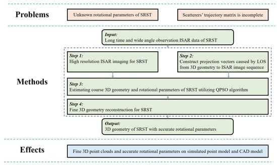
1. Introduction
2. Materials and Methods
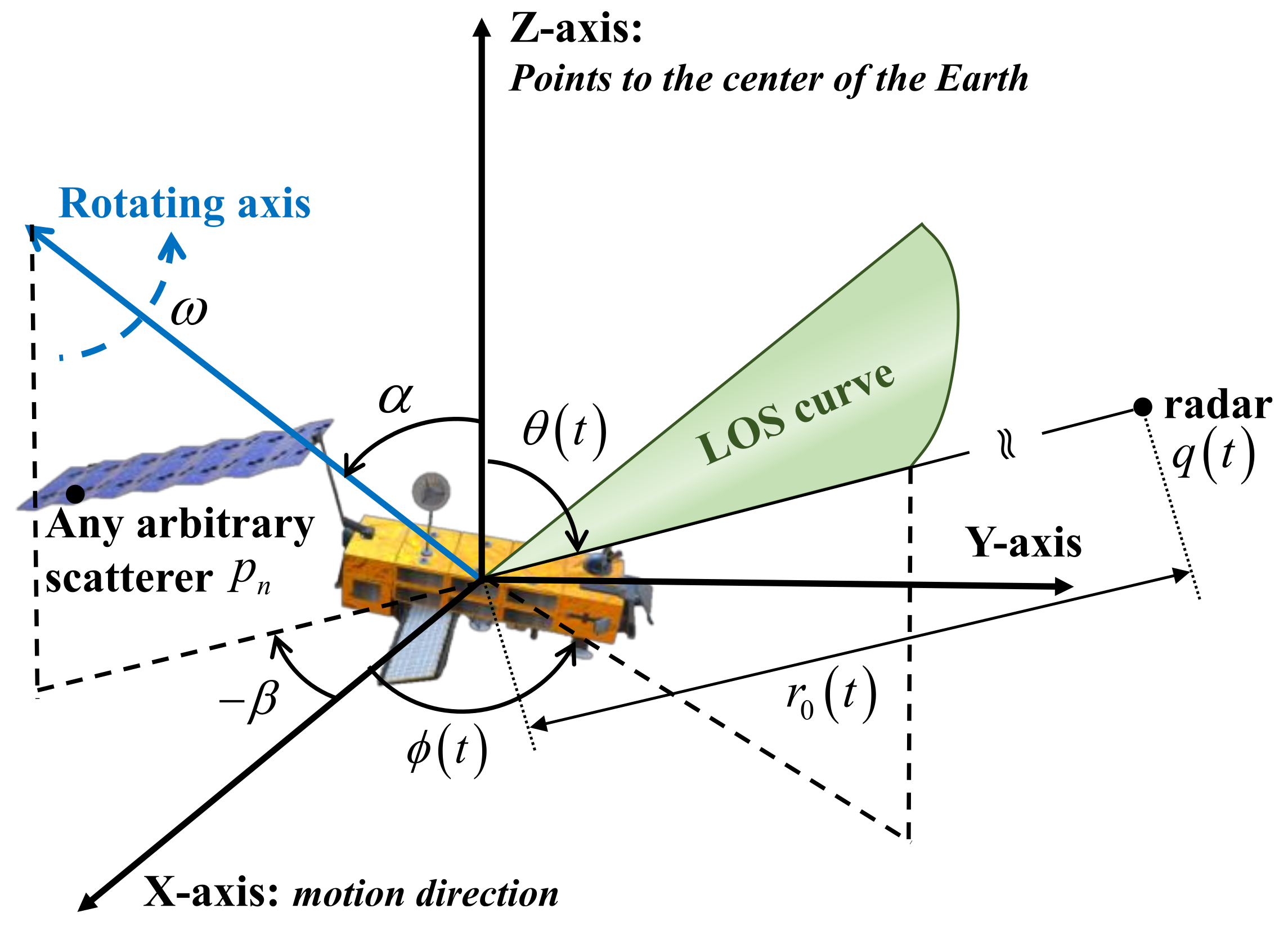
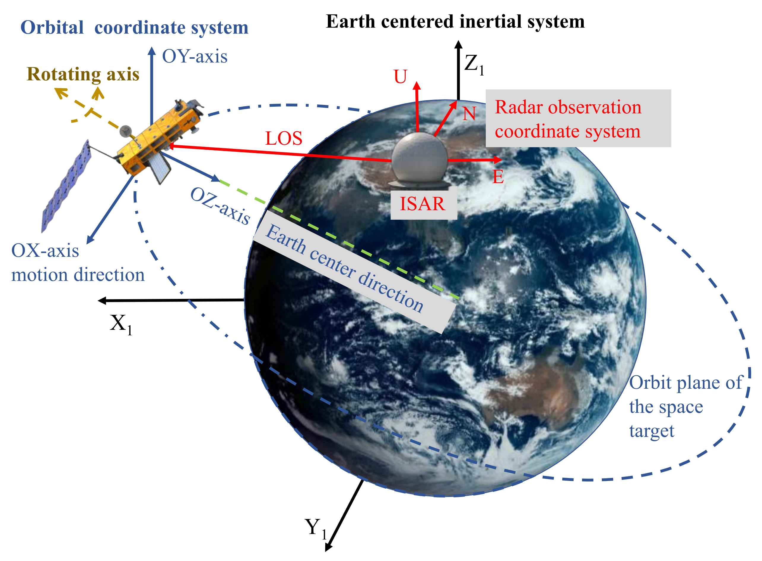
2.1. The ISAR Observation and Projection Model for Slowly Rotating Space Targets
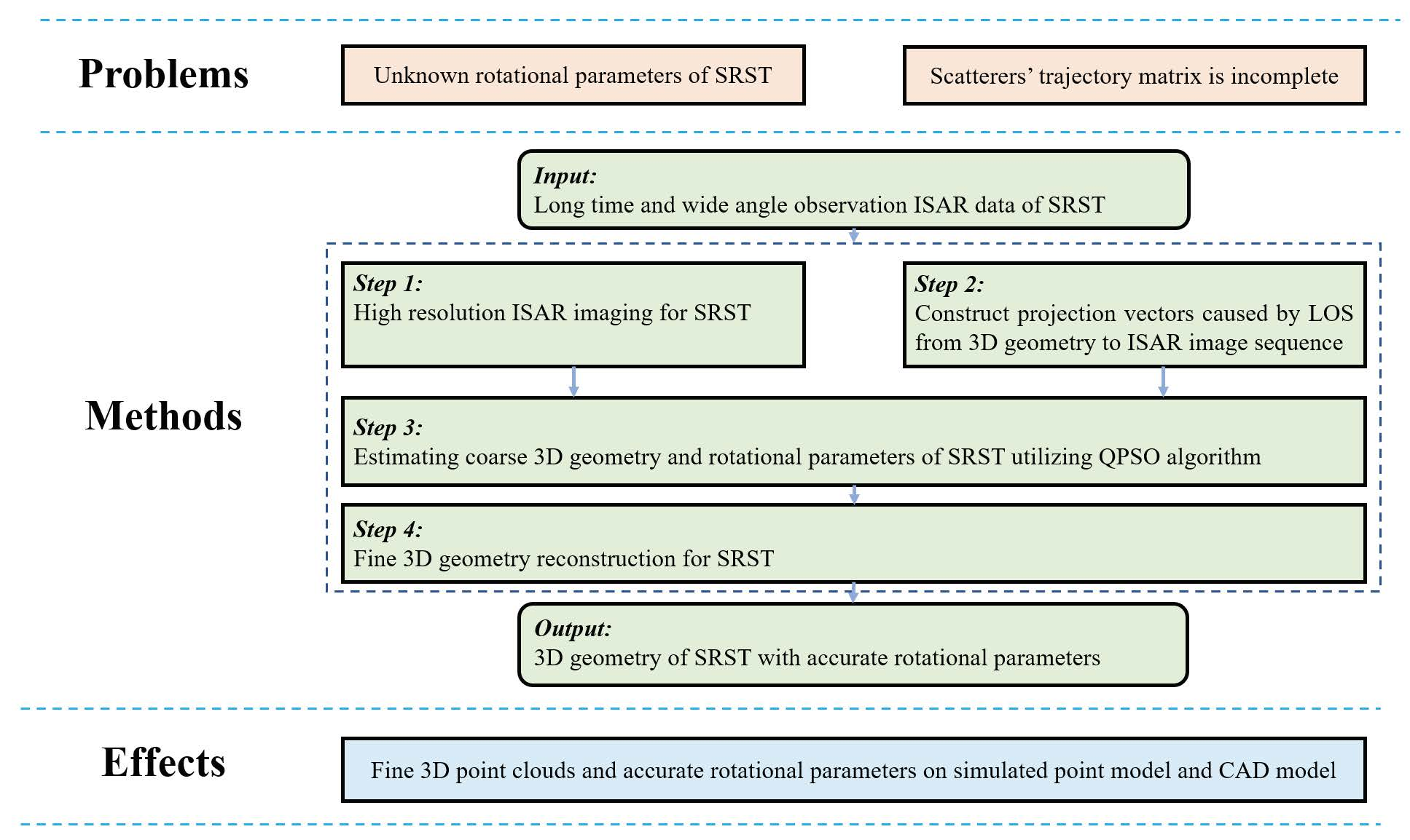
2.2. 3D Geometry Reconstruction Method for Slowly Rotating Space Targets
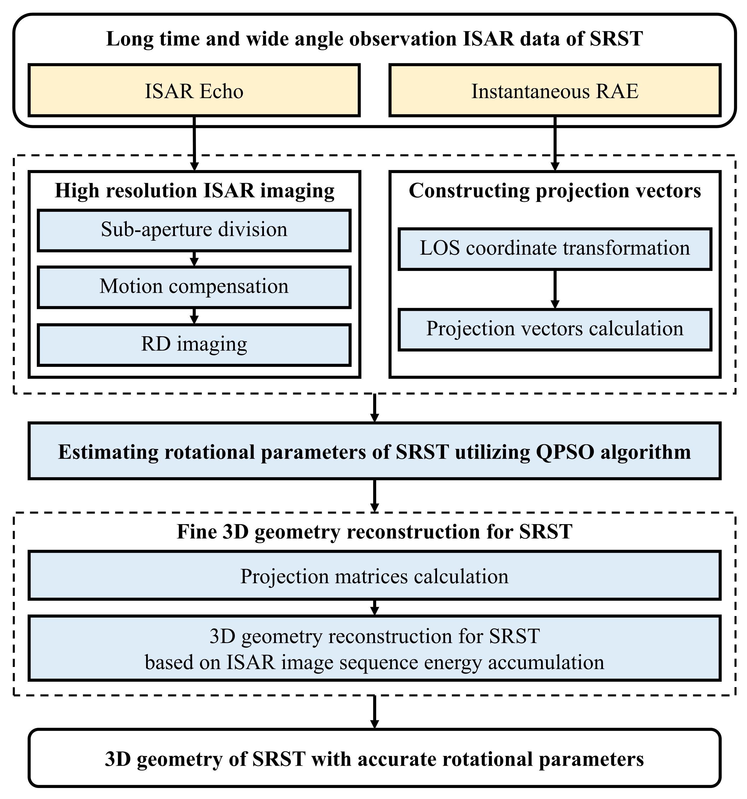
2.2.1. Algorithm Flowchart
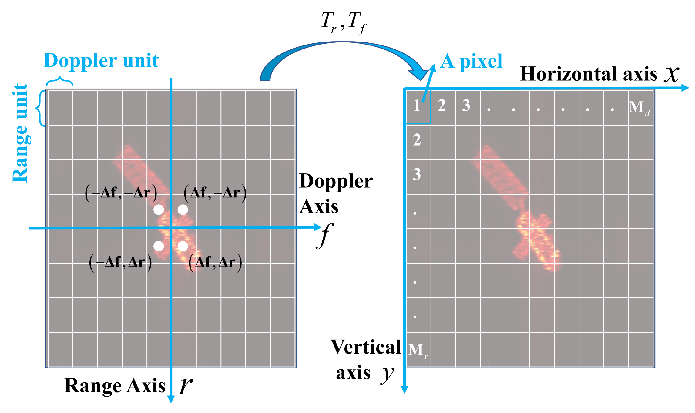
2.2.2. High Resolution ISAR Imaging for SRST
2.2.3. Constructing Projection Vectors
2.2.4. Rotational Parameters Estimation Based on the QPSO Algorithm
- Step 1: Initialization. Randomly initialize a group of particles consisting of individuals, in which the initial position of the m-th individual is . Set the individual best position of each particle . Initialize the max number of iterations as .
- Step 2: Average best position calculation. The average best position of the particle swarm can be calculated by:
- Step 3: Fitness value calculation. For each particle, construct the projection vectors via Equation (11)–(17). Then the coarse 3D geometry matrix of the SRST can be reconstructed through the ISEA method, which will be introduced in Section 2.2.5. The fitness value of each particle can be calculated by:
- Step 4: Individual best position updating. Compare the fitness value of each particle to its individual best position. If , set . Otherwise, remains.
- Step 5: Global best position updating. Set the global best position to be equal to where satisfies:
- Step 6: Individual particle position updating. Find a random position for each particle via:in which the ‘’ means that it can take a plus and a minus sign with equal probability. In addition,shows how the local best position and the global best position influence the new position of the particles. and are two random values generated from uniform distribution, i.e., . is called the shrink-expansion factor. If decreases linearly from 1 to 0.5, the QPSO usually shows better performance in the searching process.
- Step 7: Iterative stop condition. If , set and go back to step 2. Otherwise, stop the iterative process and output the global optimal position as the optimization solution.
2.2.5. 3D Geometry Reconstruction
- Step 1: Initialization. A sequence of ISAR images can be obtained via a high resolution ISAR imaging method. The projection vectors from the 3D geometry of SRST to the corresponding ISAR image sequence are constructed through Equations (11) to (17). Calculate the total energy and remaining energy of all the ISAR images. Initialize the lower limit of to 0.001, which is selected based on experiments and shows better performance. Initialize the reconstructed 3D point cloud of the SRST .
- Step 2: 3D scatterer estimation. By taking the energy of the projection positions in the ISAR image sequence as the objective function value, the 3D scatterer can be estimated via the optimization algorithms [31]. Then let .
- Step 3: Residual images updating. By taking into Equation (10), the projection positions of the 3D geometry of SRST in each ISAR image can be obtained. Also, set .
- Step 4: Iterative stop condition. Update the remaining energy of the ISAR image sequence . If , stop the iterative process and output as the reconstructed 3D point cloud. Otherwise, go back to step 2.
2.3. Performance Analysis
2.3.1. Rotational Parameter Estimation Error
2.3.2. Root-Mean-Square Error
2.3.3. Similarity of the Projection Image Sequence and ISAR Image Sequence
3. Results
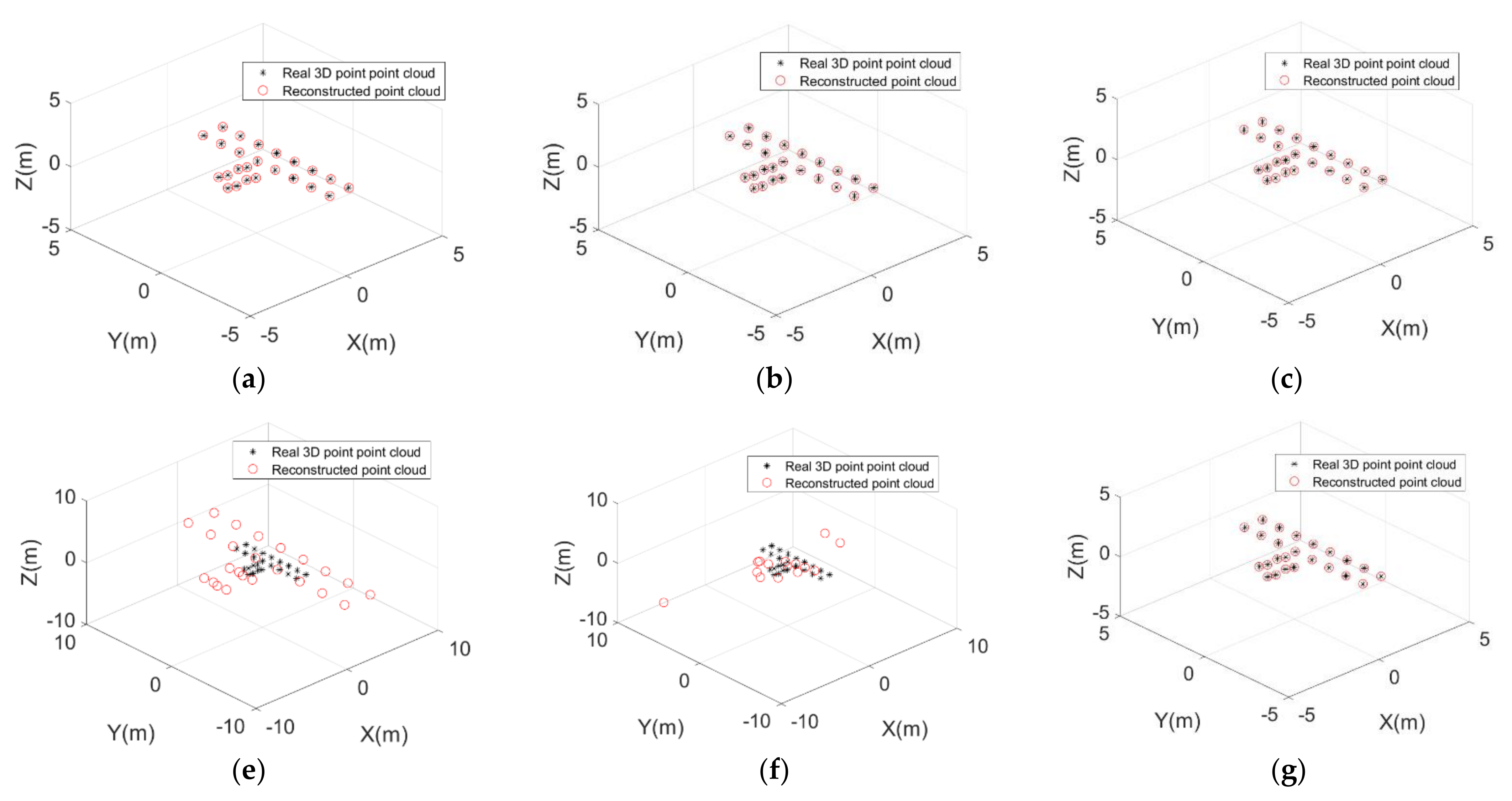
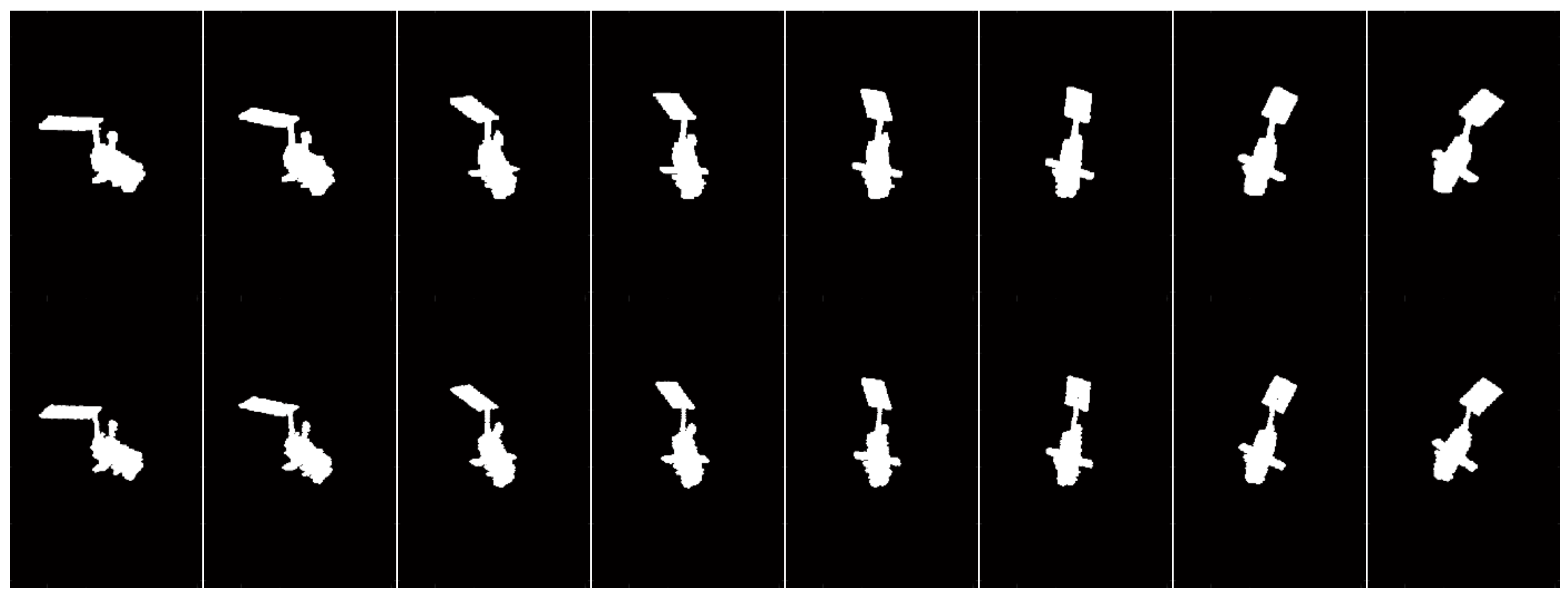
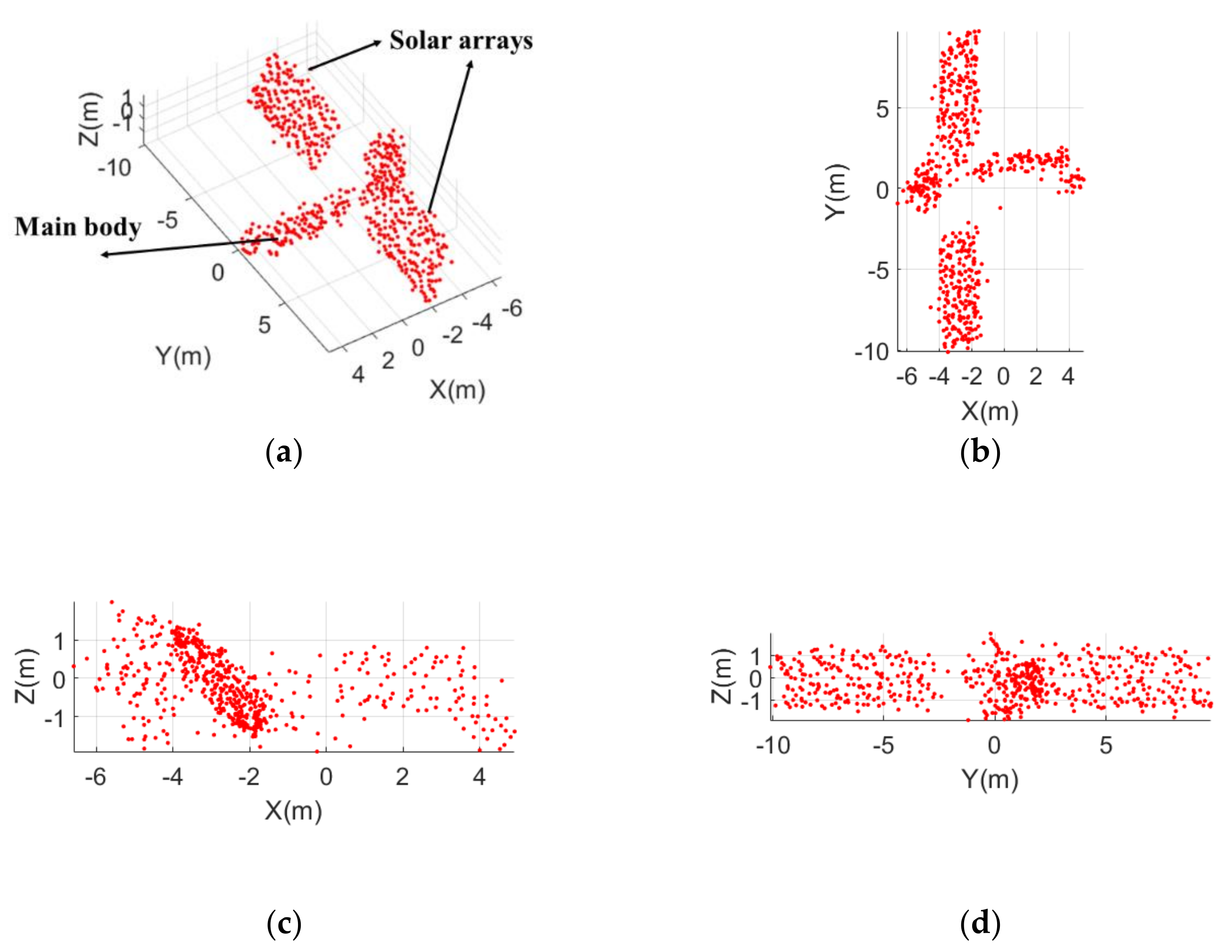
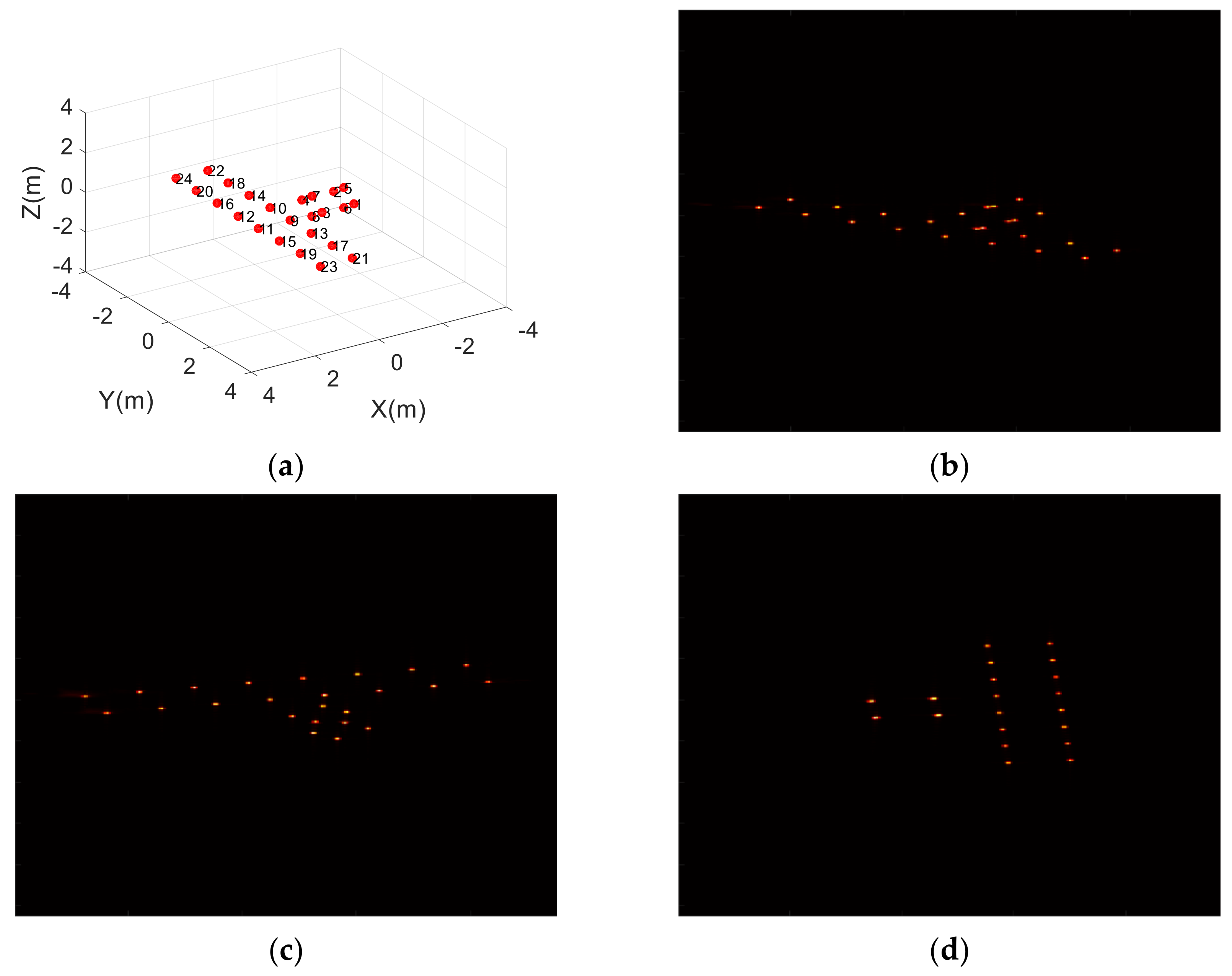
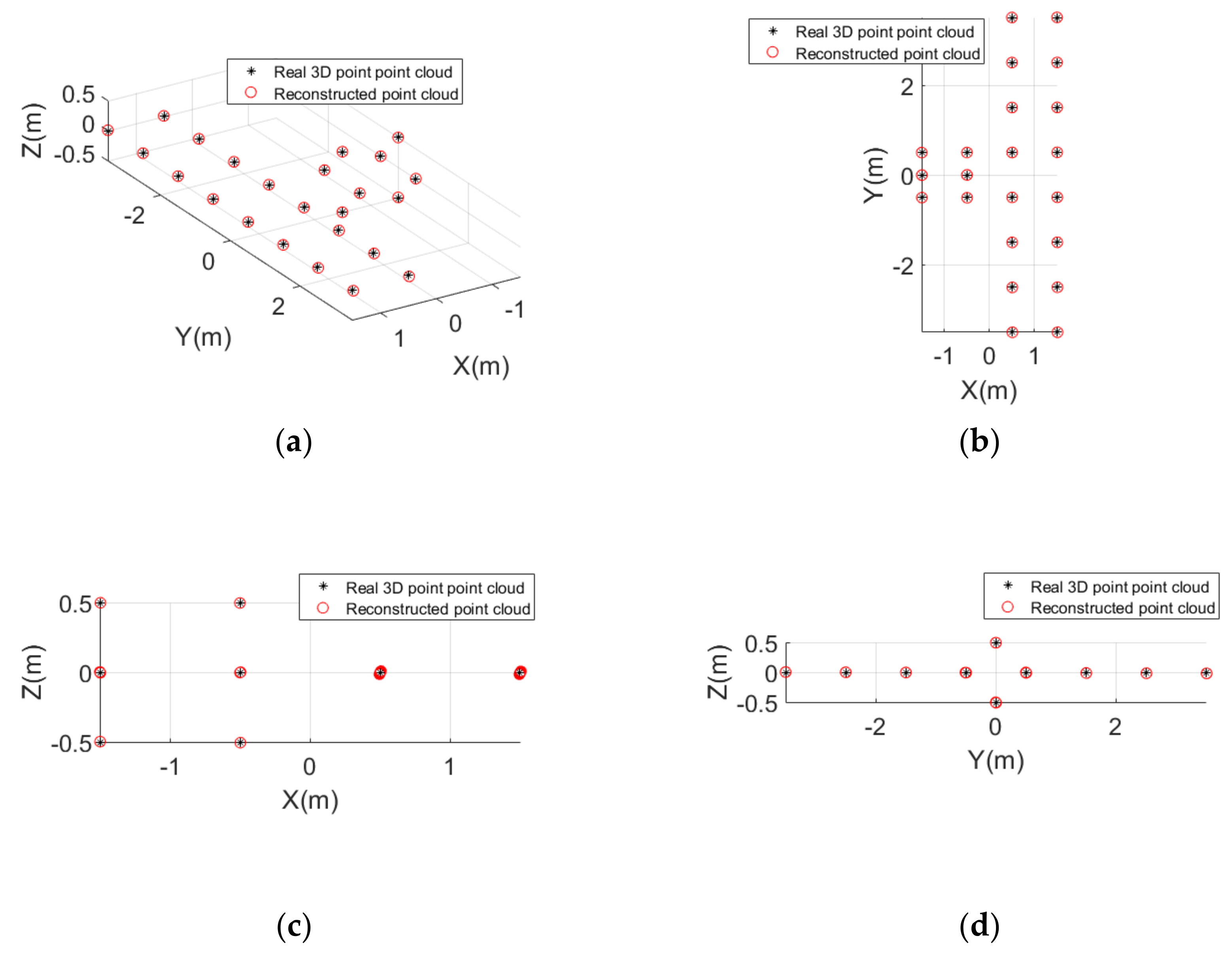
3.1. Experiment Based on a Simple Point Model of a Satellite
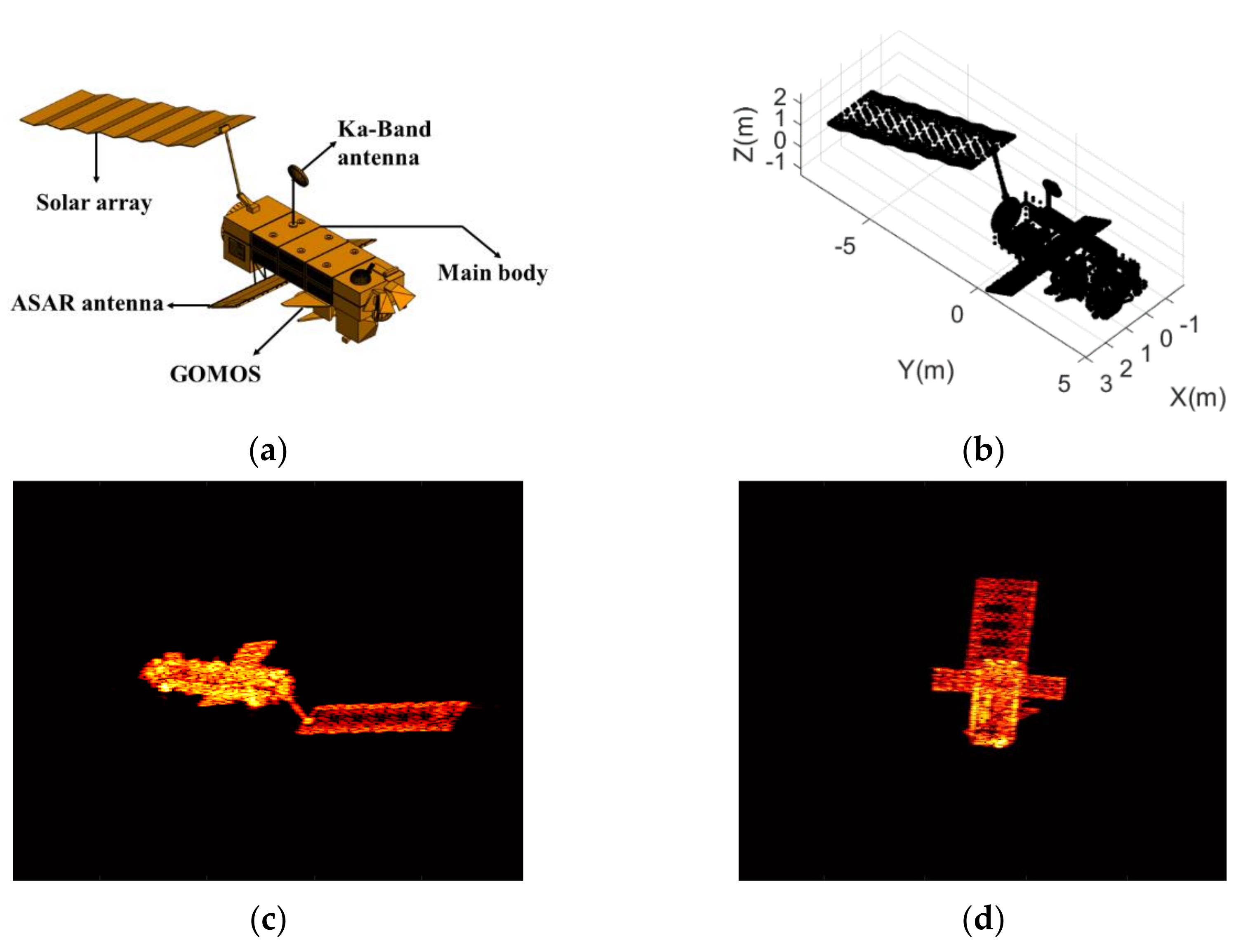
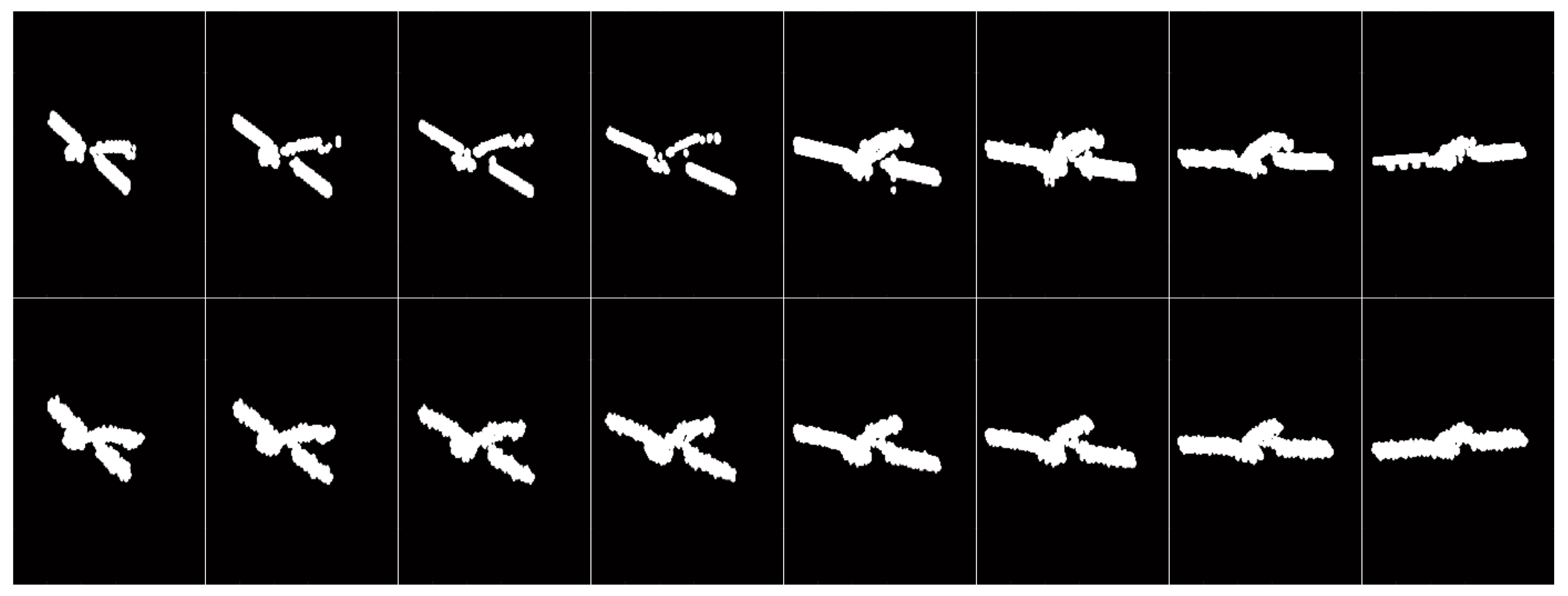
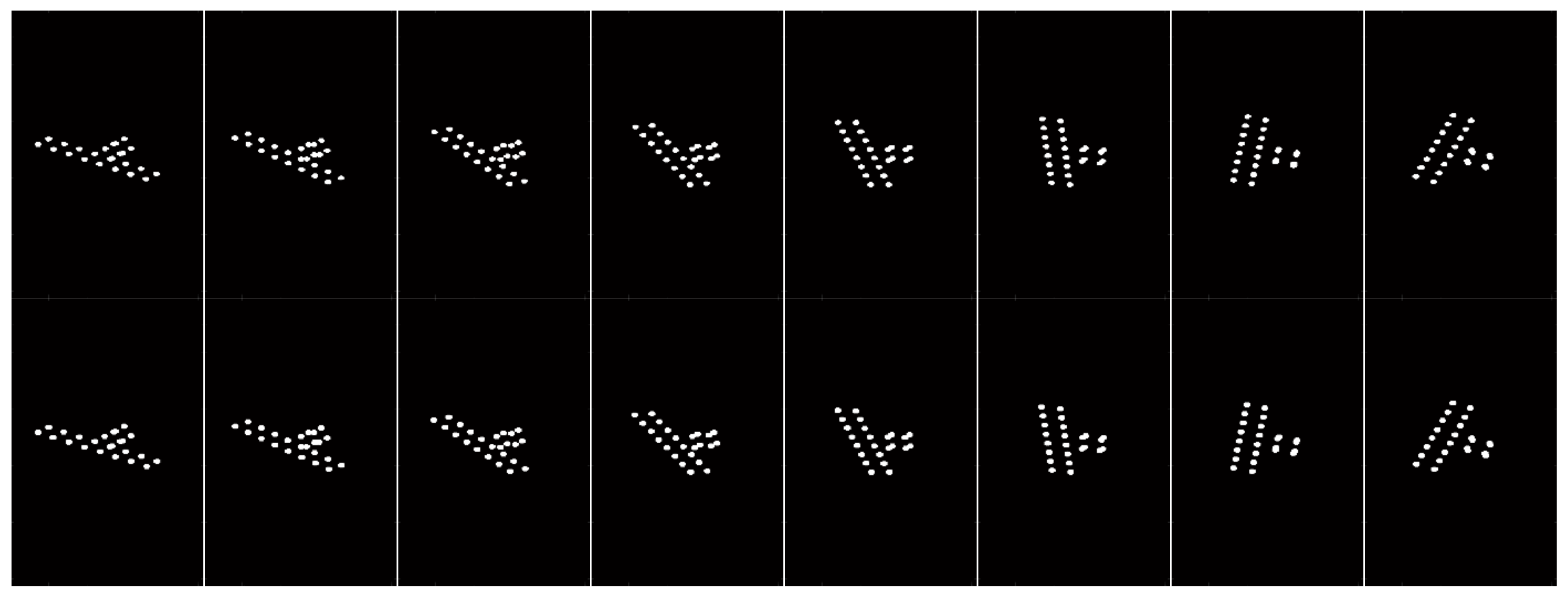
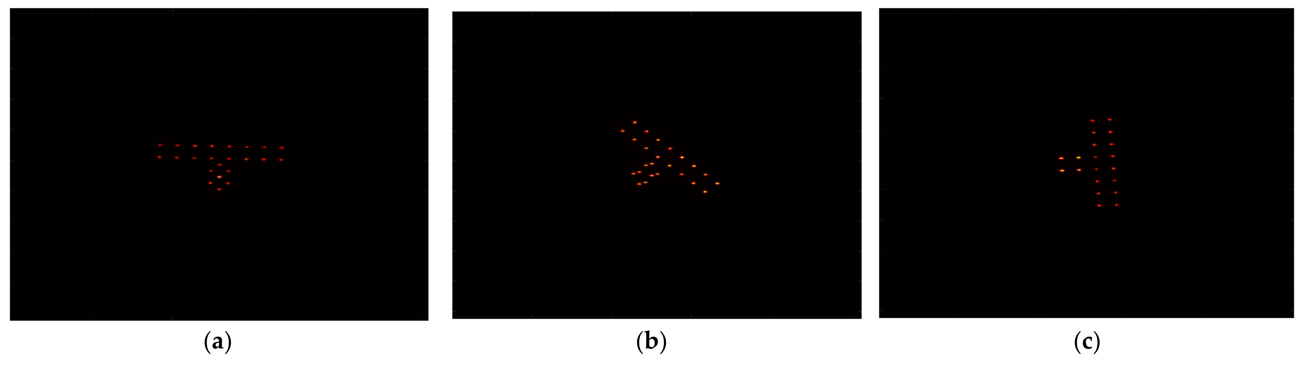
3.2. Experiment Based on a Complex Point Model of ENVISAT
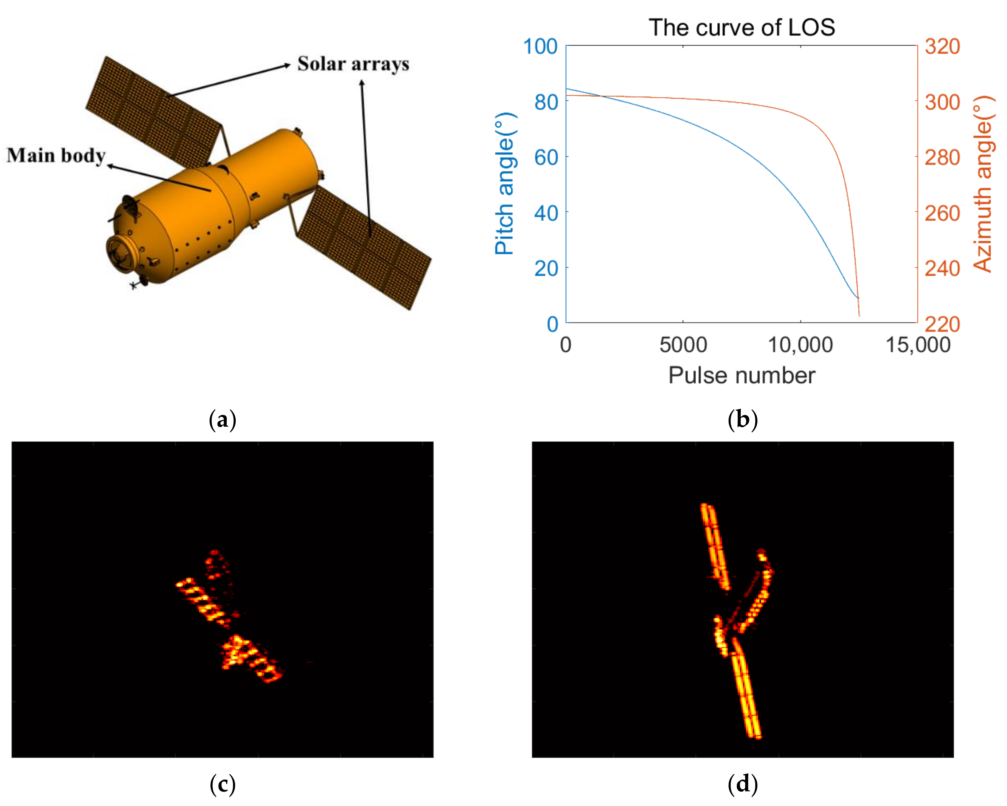
3.3. Experiment Based on Simulated Electromagnetic Data of Tiangong-1
4. Discussion
5. Conclusions
Author Contributions
Funding
Institutional Review Board Statement
Informed Consent Statement
Data Availability Statement
Acknowledgments
Conflicts of Interest
References
- Anger, S.; Jirousek, M.; Dill, S.; Peichl, M. IoSiS—A high performance experimental imaging radar for space surveillance. In Proceedings of the 2019 IEEE Radar Conference (RadarConf), Boston, MA, USA, 22–26 April 2019; pp. 1–4. [Google Scholar]
- Fonder, G.; Hughes, M.; Dickson, M.; Schoenfeld, M.; Gardner, J. Space fence radar overview. In Proceedings of the 2019 International Applied Computational Electromagnetics Society Symposium (ACES), Miami, FL, USA, 14–19 April 2019; pp. 1–2. [Google Scholar]
- Xu, G.; Yang, L.; Bi, G.; Xing, M. Maneuvering target imaging and scaling by using sparse inverse synthetic aperture. Signal Process. 2017, 137, 149–159. [Google Scholar] [CrossRef]
- Xu, G.; Yang, L.; Bi, G.; Xing, M. Enhanced ISAR imaging and motion estimation with parametric and dynamic sparse bayesian learning. IEEE Trans. Comput. Imaging 2017, 3, 940–952. [Google Scholar] [CrossRef]
- Kang, L.; Liang, B.; Luo, Y.; Zhang, Q. Sparse imaging for spinning space targets with short time observation. IEEE Sens. J. 2021, 21, 9090–9098. [Google Scholar] [CrossRef]
- Liu, M.; Zhang, X. ISAR imaging of rotating targets via estimation of rotation velocity and keystone transform. In Proceedings of the 2017 IEEE Conference on Antenna Measurements & Applications (CAMA), Tsukuba, Japan, 4–6 December 2017; pp. 265–267. [Google Scholar]
- Li, D.; Zhan, M.; Liu, H.; Liao, Y.; Liao, G. A robust translational motion compensation method for ISAR imaging based on keystone transform and fractional Fourier transform under low SNR environment. IEEE Trans. Aerosp. Electron. Syst. 2017, 53, 2140–2156. [Google Scholar] [CrossRef]
- Xin, H.-C.; Bai, X.; Song, Y.-E.; Li, B.-Z.; Tao, R. ISAR imaging of target with complex motion associated with the fractional Fourier transform. Digit. Signal Process. 2018, 83, 332–345. [Google Scholar] [CrossRef]
- Luo, X.; Guo, L.; Shang, S.; Song, D.; Li, X.; Liu, W. ISAR imaging method for non-cooperative slow rotation targets in space. In Proceedings of the 2018 12th International Symposium on Antennas, Propagation and EM Theory (ISAPE), Hangzhou, China, 3–6 December 2018; pp. 1–4. [Google Scholar]
- Yu, J.; Yang, J. Motion compensation of ISAR imaging for high-speed moving target. In Proceedings of the 2008 IEEE International Symposium on Knowledge Acquisition and Modeling Workshop, Wuhan, China, 21–22 December 2008; pp. 124–127. [Google Scholar]
- Anger, S.; Jirousek, M.; Dill, S.; Peichl, M. ISAR imaging of space objects using large observation angles. In Proceedings of the 2021 21st International Radar Symposium (IRS), Virtual, 21–22 June 2021; pp. 1–7. [Google Scholar]
- Wang, Y.; Zhang, Z.; Zhong, R.; Sun, L.; Leng, S.; Wang, Q. Densely connected graph convolutional network for joint semantic and instance segmentation of indoor point clouds. ISPRS J. Photogramm. Remote Sens. 2021, 182, 67–77. [Google Scholar] [CrossRef]
- Bassier, M.; Vergauwen, M. Topology Reconstruction of BIM Wall Objects from Point Cloud Data. Remote Sens. 2020, 12, 1800. [Google Scholar] [CrossRef]
- Zhang, L.; Li, Z.; Li, A.; Liu, F. Large-scale urban point cloud labeling and reconstruction. ISPRS J. Photogramm. Remote Sens. 2018, 138, 86–100. [Google Scholar] [CrossRef]
- Rong, J.; Wang, Y.; Han, T. Iterative optimization-based ISAR imaging with sparse aperture and its application in interferometric ISAR imaging. IEEE Sens. J. 2019, 19, 8681–8693. [Google Scholar] [CrossRef]
- Xu, D.; Xing, M.; Xia, X.-G.; Sun, G.-C.; Fu, J.; Su, T. A multi-perspective 3D reconstruction method with single perspective instantaneous target attitude estimation. Remote Sens. 2019, 11, 1277. [Google Scholar] [CrossRef] [Green Version]
- Rong, J.; Wang, Y.; Lu, X.; Han, T. InISAR imaging for maneuvering target based on the quadratic frequency modulated signal model with time-varying amplitude. IEEE Trans. Geosci. Remote Sens. 2021, 60, 5206817. [Google Scholar] [CrossRef]
- Cai, J.; Martorella, M.; Liu, Q.; Giusti, E.; Ding, Z. The alignment problem for 3D ISAR imaging with real data. In Proceedings of the 13th European Conference on Synthetic Aperture Radar, Leipzig, Germany, 29 March–1 April 2021; pp. 1–6. [Google Scholar]
- Liu, L.; Zhou, F.; Bai, X.; Tao, M.; Zhang, Z. Joint cross-range scaling and 3D geometry reconstruction of ISAR targets based on factorization method. IEEE Trans. Image Process 2016, 25, 1740–1750. [Google Scholar] [CrossRef] [PubMed]
- Zhou, C.; Jiang, L.; Yang, Q.; Ren, X.; Wang, Z. High precision cross-range scaling and 3D geometry reconstruction of ISAR targets based on geometrical analysis. IEEE Access 2020, 8, 132415–132423. [Google Scholar] [CrossRef]
- Wang, F.; Xu, F.; Jin, Y.Q. Three-dimensional reconstruction from a multiview sequence of sparse ISAR imaging of a space target. IEEE Trans. Geosci. Remote Sens. 2018, 56, 611–620. [Google Scholar] [CrossRef]
- Yang, S.; Jiang, W.; Tian, B. ISAR image matching and 3D reconstruction based on improved SIFT method. In Proceedings of the 2019 International Conference on Electronic Engineering and Informatics (EEI), Nanjing, China, 8–10 November 2019; pp. 224–228. [Google Scholar]
- Kang, L.; Luo, Y.; Zhang, Q.; Liu, X.; Liang, B. 3D scattering image reconstruction based on measurement optimization of a radar network. Remote Sens. Lett. 2020, 11, 697–706. [Google Scholar] [CrossRef]
- Kang, L.; Luo, Y.; Zhang, Q.; Liu, X.; Liang, B. 3-D Scattering Image Sparse Reconstruction via Radar Network. IEEE Trans. Geosci. Remote Sens. 2021, 60, 5100414. [Google Scholar] [CrossRef]
- Tomasi, C.; Kanade, T. Shape and motion from image streams: A factorization method. Proc. Natl. Acad. Sci. USA 1993, 90, 9795–9802. [Google Scholar] [CrossRef] [Green Version]
- Leutenegger, S.; Chli, M.; Siegwart, R.Y. BRISK: Binary robust invariant scalable keypoints. In Proceedings of the 2011 International Conference on Computer Vision, Barcelona, Spain, 6–13 November 2011; pp. 2548–2555. [Google Scholar]
- Di, G.; Su, F.; Yang, H.; Fu, S. ISAR image scattering center association based on speeded-up robust features. Multimed. Tools. Appl. 2018, 79, 5065–5082. [Google Scholar] [CrossRef]
- Liu, L.; Zhou, F.; Bai, X. Method for scatterer trajectory association of sequential ISAR images based on Markov chain Monte Carlo algorithm. IET Radar, Sonar Navig. 2018, 12, 1535–1542. [Google Scholar] [CrossRef]
- Du, R.; Liu, L.; Bai, X.; Zhou, F. A New Scatterer Trajectory Association Method for ISAR Image Sequence Utilizing Multiple Hypothesis Tracking Algorithm. IEEE Trans. Geosci. Remote Sens. 2022, 60, 5103213. [Google Scholar] [CrossRef]
- Liu, L.; Zhou, F.; Bai, X.; Paisley, J.; Ji, H. A modified EM algorithm for ISAR scatterer trajectory matrix completion. IEEE Trans. Geosci. Remote Sens. 2018, 56, 3953–3962. [Google Scholar] [CrossRef]
- Liu, L.; Zhou, Z.; Zhou, F.; Shi, X. A new 3-D geometry reconstruction method of space target utilizing the scatterer energy accumulation of ISAR image sequence. IEEE Trans. Geosci. Remote Sens. 2020, 58, 8345–8357. [Google Scholar] [CrossRef]
- Bai, X.; Zhou, F. Radar Imaging of Micromotion Targets from Corrupted Data. IEEE Trans. Aerosp. Electron. Syst. 2016, 52, 2789–2802. [Google Scholar] [CrossRef]
- Bai, X.; Zhou, F.; Bao, Z. High-Resolution Three-Dimensional Imaging of Space Targets in Micromotion. IEEE J. Sel. Top. Appl. Earth Obs. Remote Sens. 2015, 8, 3428–3440. [Google Scholar] [CrossRef]
- Sommer, S.; Rosebrock, J.; Cerutti-Maori, D. Temporal analysis of ENVISAT’s rotational motion. In Proceedings of the 7th European Conference on Space Debris, Darmstadt, Germany, 18–21 April 2017; pp. 1–3. [Google Scholar]
- Lab, F. Monitoring the Re-Entry of the Chinese Space Station Tiangong-1 with TIRA. Available online: https://www.fhr.fraunhofer.de/en/businessunits/space/monitoring-the-re-entry-of-the-chinese-space-station-tiangong-1-with-tira.html (accessed on 1 April 2018).
- Taubin, G. 3D rotations. IEEE Comput. Graph. Appl. 2011, 31, 84–89. [Google Scholar] [CrossRef] [PubMed]
- Liu, Y.; Yi, D.; Wang, Z. Coordinate transformation methods from the Inertial System to the Centroid Orbit System. Aerosp. Control 2007, 25, 4–8. [Google Scholar] [CrossRef]
- Bergh, F.V.D.; Engelbrecht, A.P. A new locally convergent particle swarm optimiser. In Proceedings of the IEEE International Conference on Systems, Man and Cybernetics, Yasmine Hammamet, Tunisia, 6–9 October 2002; pp. 1–6. [Google Scholar]
- Jun, S.; Wenbo, X.; Bin, F. A global search strategy of quantum-behaved particle swarm optimization. In Proceedings of the 2004 IEEE Conference on Cybernetics and Intelligent Systems, Singapore, 1–3 December 2004; pp. 111–116. [Google Scholar]
- Sun, J.; Feng, B.; Xu, W. Particle swarm optimization with particles having quantum behavior. In Proceedings of the 2004 Congress on Evolutionary Computation (IEEE Cat. No.04TH8753), Portland, OR, USA, 19–23 June 2004; pp. 325–331. [Google Scholar]
- Sun, J.; Wang, W.; Wu, X.; Xu, W. Quantum-Behaved Particle Swarm Optimization Principle and Application, 1st ed.; Tsinghua University Press: Beijing, China, 2011; pp. 31–51. [Google Scholar]
- Agency, E.S. ENVISAT Instruments. Available online: https://earth.esa.int/eogateway/missions/envisat (accessed on 27 November 2021).


| Parameters | Value |
|---|---|
| Duration of observation | 100 s |
| Number of ISAR images | 48 |
| Observation azimuth angle | 0°–180° |
| Observation pitch angle | 45° |
| Rotational Parameters | Rotational Velocity (rad/s) | Pitch Angle of the Rotational Axis (°) | Azimuth Angle of the Rotational Axis (°) |
|---|---|---|---|
| Real value | −0.05236 | 10 | 5 |
| Estimated value | −0.05247 | 10.1702 | 6.2495 |
| Error | 1.1 × 10⁻⁴ | 0.2772 | |
| Targets Status | Evaluation Values | The Factorization Method | The ISEA Method | The Proposed Method |
|---|---|---|---|---|
| Non-rotating | RMSE (m) | 0.0183 | 0.0068 | 0.0091 |
| Image similarity | 0.9321 | 0.9458 | 0.9451 | |
| Slowly rotating | RMSE (m) | - | - | 0.0082 |
| Image similarity | 0.0410 | 0.2871 | 0.9330 |
| Rotational Parameters | Rotational Velocity (rad/s) | Pitch Angle of the Rotational Axis (°) | Azimuth Angle of the Rotational Axis (°) |
|---|---|---|---|
| Real value | −0.05236 | 10 | 5 |
| Estimated value | −0.05234 | 9.9430 | 6.0751 |
| Error | 2 × 10⁻⁵ | 0.1947 | |
| Rotational Parameters | Rotational Velocity (rad/s) | Pitch Angle of the Rotational Axis (°) | Azimuth Angle of the Rotational Axis (°) |
|---|---|---|---|
| Real value | −0.05236 | 130 | 120 |
| Estimated value | −0.05269 | 130.3217 | 120.5304 |
| Error | 3.3 × 10⁻⁴ | 0.5175 | |
Publisher’s Note: MDPI stays neutral with regard to jurisdictional claims in published maps and institutional affiliations. |
© 2022 by the authors. Licensee MDPI, Basel, Switzerland. This article is an open access article distributed under the terms and conditions of the Creative Commons Attribution (CC BY) license (https://creativecommons.org/licenses/by/4.0/).
Share and Cite
Zhou, Z.; Liu, L.; Du, R.; Zhou, F. Three-Dimensional Geometry Reconstruction Method for Slowly Rotating Space Targets Utilizing ISAR Image Sequence. Remote Sens. 2022, 14, 1144. https://doi.org/10.3390/rs14051144
Zhou Z, Liu L, Du R, Zhou F. Three-Dimensional Geometry Reconstruction Method for Slowly Rotating Space Targets Utilizing ISAR Image Sequence. Remote Sensing. 2022; 14(5):1144. https://doi.org/10.3390/rs14051144
Chicago/Turabian StyleZhou, Zuobang, Lei Liu, Rongzhen Du, and Feng Zhou. 2022. "Three-Dimensional Geometry Reconstruction Method for Slowly Rotating Space Targets Utilizing ISAR Image Sequence" Remote Sensing 14, no. 5: 1144. https://doi.org/10.3390/rs14051144
APA StyleZhou, Z., Liu, L., Du, R., & Zhou, F. (2022). Three-Dimensional Geometry Reconstruction Method for Slowly Rotating Space Targets Utilizing ISAR Image Sequence. Remote Sensing, 14(5), 1144. https://doi.org/10.3390/rs14051144