Article

Deterioration Mapping of RC Bridge Elements Based on Automated Analysis of GPR Images

1
Department of Building, Civil and Environmental Engineering, Concordia University, 1455 De Maisonneuve Blvd. W., Montreal, QC H3G 1M8, Canada
2
Department of Building and Real Estate, The Hong Kong Polytechnic University, Hong Kong 853H, China
*
Author to whom correspondence should be addressed.
Remote Sens. 2022, 14(5), 1131; https://doi.org/10.3390/rs14051131
Submission received: 9 January 2022 / Revised: 22 February 2022 / Accepted: 23 February 2022 / Published: 25 February 2022

Abstract

:
Ground-Penetrating Radar (GPR) is a popular non-destructive technique for evaluating RC bridge elements as it can identify major subsurface defects within a short span of time. The data interpretation of the GPR profiles based on existing amplitude-based approaches is not completely reliable when compared to the actual condition of concrete with destructive measures. An alternative image-based analysis considers GPR as an imaging tool wherein an experienced analyst marks attenuated areas and generates deterioration maps with greater accuracy. However, this approach is prone to human errors and is highly subjective. The proposed model aims to improve it through automated detection of hyperbolas in GPR profiles and classification based on mathematical modeling. Firstly, GPR profiles are pre-processed, and hyperbolic reflections were detected in them based on a trained classifier using the Viola–Jones Algorithm. The false positives are eliminated, and missing regions are identified automatically across the top/bottom layer of reinforcement based on user-interactive regional comparison and statistical analysis. Subsequently, entropy, a textural factor, is evaluated to differentiate the detected regions closely equivalent to the human visual system. These detected regions are finally clustered based on entropy values using the K-means algorithm and a deterioration map is generated which is robust, reliable, and corresponds to the in situ state of concrete. A case study of a parking lot demonstrated good correspondence of deterioration maps generated by the developed model when compared with both amplitude- and image-based analysis. These maps can facilitate structural inspectors to locally identify deteriorated zones within structural elements that require immediate attention for repair and rehabilitation.

Graphical Abstract

1. Introduction

Reliable condition assessment of reinforced concrete elements of a bridge or any structure is crucial for its regular repair, rehabilitation, and overall sustainability. The oldest yet most widely popular approach for inspecting bridge elements involves an experienced analyst visually identifying and rating the surface defects based on their condition [1]. However, such a visual inspection method does not detect subsurface defects such as corrosion, voids, and delamination. Therefore, the use of non-destructive techniques (NDTs) is being increasingly adopted by transportation authorities for rigorous health evaluation of a bridge element. Although there are various NDTs such as impact echo, infrared thermography (IR), Ground-Penetrating Radar (GPR), Ultrasonic Surface Waves (USW) among others, GPR is the most recommended and highest-rated NDT among all as it can identify major subsurface defects (delamination, corrosion, vertical cracks, and concrete degradation) within a short span of time [2].
In essence, the GPR technique involves emitting electromagnetic radar signals through scanning a bridge element and analyzing the recorded signals [3]. The data interpretation of these recorded signals or GPR profiles is typically based on analyzing amplitude values at various medium interfaces such as asphalt–concrete or concrete–rebars to determine rebar corrosion, cover depth, and other factors. ASTM D6087 has a standardized procedure to evaluate asphalt-covered bridge decks based on such amplitude values [4]. However, the deterioration maps developed based on such amplitude values are not totally reliable when compared with the actual condition of concrete using destructive techniques such as core sampling [5]. To overcome the limitations of the amplitude-based analysis, a visual image-based analysis (IBA) method was proposed by Tarussov et al., 2013 [5]. In this approach, an experienced analyst manually marks the attenuated areas in GPR profiles while considering various anomalies to generate deterioration maps with a fair degree of accuracy.
The IBA method, however, suffers from the following limitations: it is subjective, time-consuming, and prone to human error as the analysis is performed manually [6]. This study aims to reduce the subjectivity of this method through automation and scientific analysis of GPR profiles. It is achieved through these steps: (a) firstly, the hyperbolic variations are detected in GPR profiles using the Viola–Jones Algorithm and statistical analysis [7], (b) a texture-based factor is evaluated for the detected objects, and (c) a K-means algorithm is utilized to cluster the evaluated factors into three or four regions corresponding to concrete deterioration levels ranging from good to bad. The condition assessment maps generated based on this developed model are robust, reliable, and correspond to the real in situ state of concrete. It would facilitate bridge inspectors in making informed decisions with regard to repair, rehabilitation, or replacement of bridge elements.

2. Objectives of Research

The overall objective of this study is to develop a model for reliable deterioration maps based on automated IBA of GPR profiles. The following enumerates a breakdown of milestones achieved while developing the model:
  • A review of the GPR scanning procedure and its data interpretation methods including the widely used amplitude-based approach.
  • An overview of IBA, its advantages, and current limitations.
  • A summary of the Viola–Jones Algorithm for hyperbola detections.
  • Develop a new model to generate a deterioration map based on automated detections, textural factors, and clustering.
  • Comparison of maps generated by the developed model with two existing approaches using a RC slab case study.

3. Research Background

The first step in assessment using GPR involves scanning the structure such as a bridge element or a pavement with a mobile or manually driven antenna that emits electromagnetic (EM) waves. A manual-driven cart is preferred for a detailed survey while a mobile or airborne survey is opted for reconnaissance. Typically, the scanning is conducted either along the longitudinal section of the element or in a grid pattern with uniform traverse spacing to cover the whole element. The traverse spacing between each scan depends upon the aim of the investigation such as the level of details needed. For example, to map detailed features of a bridge deck, spacing of 1 to 2 feet is utilized while 3 to 6 feet is generally used for a reconnaissance or quality-assurance survey [8]. The antenna frequency for GPR scanning typically varies from 1 to 5 GHz and is decided based on the resolution needed for the survey and the penetration depth. Generally, a higher antenna frequency provides higher resolution power but lower penetration depth and vice versa [9]. Several other parameters for the GPR survey such as the number of samples per scan, transmit rate, number of scans per unit of distance, and dielectric constant are pre-set based on the investigation needed [8].
The EM signals emitted from the GPR frequency antenna are reflected at various material interfaces and are recorded by the GPR equipment. The output signal at a particular point, called the A-scan, is proportional to its amplitude. When these A-scans are stacked together along the length of the survey scan, it represents a greyscale image called a B-Scan [10]. Figure 1 shows a typical B-Scan of a concrete bridge deck with asphalt overlay with distinct reflections at various interfaces: air/asphalt, asphalt/concrete, and concrete–rebar. The reflections at the concrete–rebar interface form a characteristic hyperbolic shape and its peak represents the embedded rebar location in concrete.

3.1. GPR Data Analysis

Several methods have been proposed in the literature to interpret data obtained from GPR scans. The earliest approach identified irregular signatures in profiles as concrete deterioration typically present in a depressed shape [11]. Subsequently, individual waveforms at the concrete/asphalt level were analyzed in several bridge decks and a rating system was developed to classify the deck condition [12,13]. Numerous researchers analyzed attenuation signals based on amplitude values and compared their effectiveness in measuring concrete deterioration [14,15,16,17,18]. To improve results of amplitude-based analysis, the following advances were proposed: (a) analyzed signal depth–amplitude effects [19], (b) measured change in amplitude values over time [10], and (c) correlated original waveforms with semi-simulated waveforms at deterioration state [20]. An experimental study was conducted to assess the reliability of GPR in detecting delamination [21]. Some recent methods for complete data assessment can be summarized as follows: (a) analyzed amplitude values with synthetic aperture focusing technique (SAFT) and 3D interpolation [22], (b) compared A-scans at different locations [23], (c) utilized step-frequency GPR antenna arrays [24], (d) applied frequency–wavenumber (F–K) migration and several other algorithms to detect major defects (delamination, air voids and moisture) [25], (e) statistically analyzed concrete relative permittivity over multiple years [26], (f) evaluated three parameters (direct-coupling, amplitude, wave velocity, and signal attenuation) at different depths [27], and (g) used dual-polarization antenna for scanning and developed SAFT-based algorithms for 3D imaging of concrete structures to detect objects, defects, steel bar debonding, and concrete delamination [28].
The commonly adopted approach by transportation authorities to analyze GPR data is based on ASTM D6087 [4]. After obtaining GPR profiles from scanning a bridge element required to be inspected, this method involves picking reflection amplitude values in regular intervals across B-scans at either of the two locations: (a) concrete–rebar interface, i.e., the peak of hyperbolas or (b) relative amplitudes from the bridge deck bottom relative to the bridge deck surface. Subsequently, a condition map is generated for the complete bridge element by mapping these amplitude values. Higher values of amplitudes in this map indicate locations of good conditions of concrete while lower values indicate locations of moderate-to-bad conditions of the concrete. Bridge inspectors can use such a map to identify deteriorated areas for further inspection and repairs.

3.2. Visual Image-Based Analysis
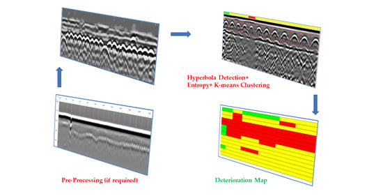
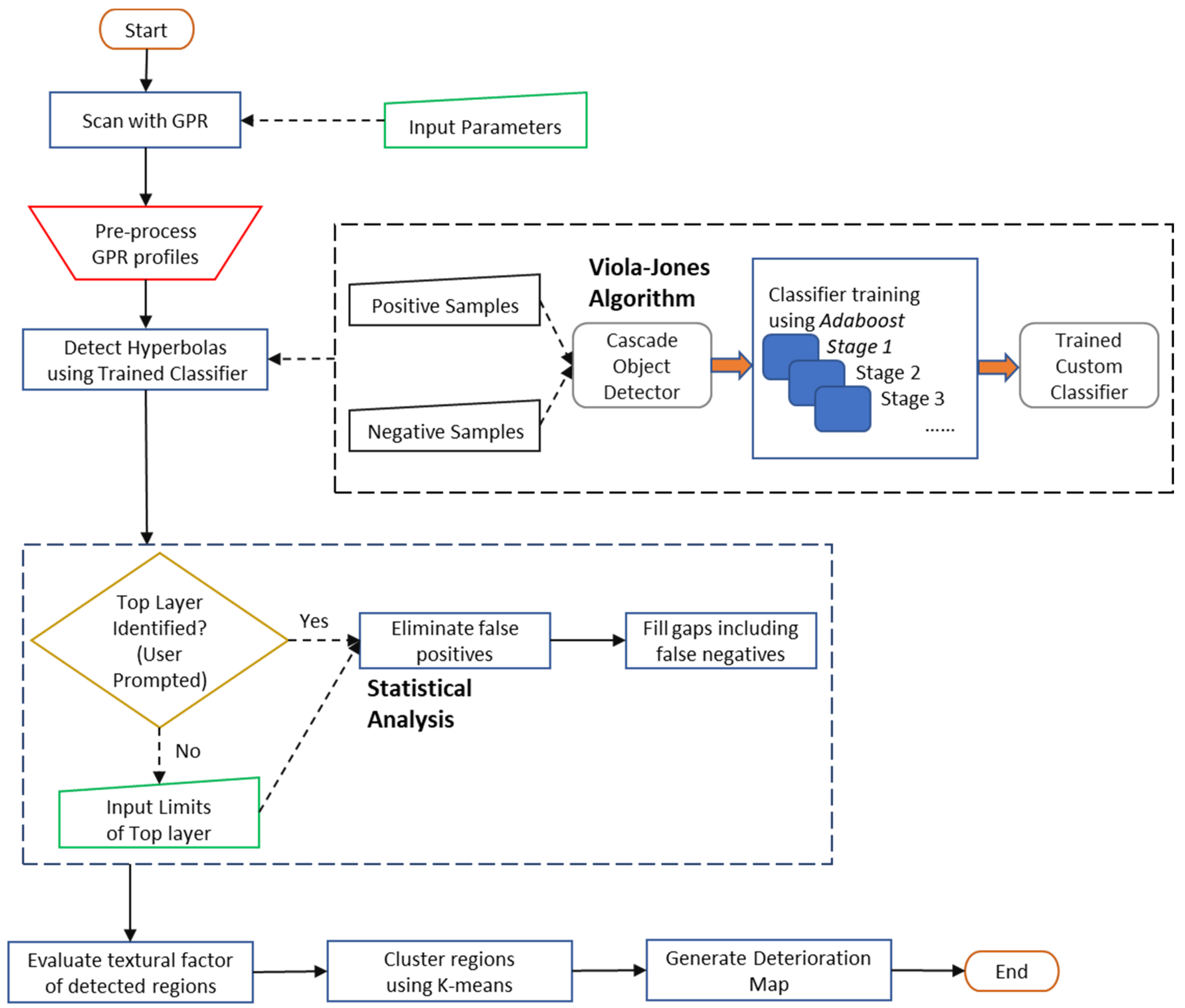
The methods based on numerical amplitude values have many limitations. Firstly, by considering only amplitude values in a B-scan, they ignore the majority of the information contained in a radar profile. Secondly, they can yield erroneous results due to factors affecting amplitudes such as depth, surface anomalies, reinforcing bar spacing/configuration, and others. Thirdly, the condition map generated is noisy and not completely reliable when compared with the actual condition of concrete with destructive measures such as core sampling [5]. To overcome these shortcomings, an alternative approach proposed by Tarussov et al., 2013 [5] considers GPR B-scans as an imaging tool rather than a numeral measuring tool. In this visual-IBA, an experienced analyst marks attenuated areas in a B-scan manually while considering several factors such as reflection amplitudes at the concrete/rebar and bottom of slab levels, surface and structural anomalies, variations in slab thickness, reinforcement bar spacing, etc. For example, Figure 2 shows a typical GPR profile wherein moderate zones of deterioration are marked in yellow color by the analyst on top of the profile while severe zones are marked in red. The deterioration maps generated based on this approach have the following benefits: (a) it maps exact limits for zones of corrosion; (b) it reduces noise in results through visual filtering; (c) it accounts for depth-correction; (d) it considers various surface and structural anomalies as stated before; and (e) it shows good correspondence when compared with ground-truth results.
The IBA method was correlated with extracted cores (destructive technique), chain-drag and chloride profiles on sets of concrete bridge decks scanned using GPR along a section of the I-290 and I-294 Tollways in Chicago, IL, USA. The corrosion maps generated during this investigation showed better correspondence with the actual concrete condition [5]. Abouhamad et al., 2017 [29] proposed a systematic framework to develop corrosion maps based on visual-IBA method by Tarussov et al., 2013 [5]. The developed IBA framework was validated by scanning two bridge decks in Quebec and comparing the resultant maps with amplitude-based maps, visual inspection, ground-truth cores and Half-Cell Potential (HCP). Dawood et al., 2020 [30] proposed an integrated approach to develop deterioration maps which delineates air/water voids in subway tunnels based on the GPR-IBA framework [29]. A part of Montreal, Quebec subway tunnel was inspected, and the map generated by the developed model [30] showed high correlation when compared with laser-based thermal map, visual inspection (camera images), and extracted cores. Therefore, the visual-IBA method philosophy was adopted in the proposed model instead of amplitude-based approaches due to better correspondence with the ground truth condition. However, this method has a few limitations of its own [6]. Primarily, since an analyst marks the attenuated areas manually, it is prone to human errors. For example, an analyst could mark a particular area in a B-scan differently each time as moderate or severe based on his/her optic judgment. Secondly, different analysts could have varied visual perspectives of what constitute areas in GPR profiles as good, moderate, or bad; and therefore, it is subjective. Lastly, the method could be time-consuming and tiresome especially in cases of bridge decks with large spans. This paper overcomes the limitations of the visual-IBA method through automated detections of hyperbolas and classification based on mathematical modeling. A condition map generated using the developed model would yield a consistent (same) result for a given set of GPR data devoid of any human errors.
The premier step, detection of hyperbolas in GPR profiles, has been the focus of various researchers in analyzing GPR data. These methods utilize a variety and combination of image processing techniques such as edge detection, thresholding, and template matching. There are several limitations in employing such techniques; for example, edge detection or thresholding involves a pre-defined automatic or manual “threshold” which could lead to noise and non-uniform results across a variety of GPR profiles. Template matching causes missing or false detections of hyperbolas and requires a large database to incorporate the diversity of the shape of hyperbolas. Initial techniques of detecting hyperbola involved direct curve fitting such as Hough transform [31,32], wavelets [33,34], radon transforms [35], and hyperbolic echo characteristics [36]. A smart algorithm identified ill-shaped hyperbolas as it accounted for misshapenness by considering a buffer zone [37]. Some methods have used neural networks [38,39,40,41], while a few have adopted pattern-recognition algorithms [42,43,44]. Peak detection was also achieved by fuzzy clustering [45] and a multi-objective genetic algorithm [46]. Two holistic methods generated deterioration maps through automated rebar picking of amplitude values [47,48]. Some of the latest approaches to distinguishing hyperbolic regions from the background have been developed based on following algorithms: (a) a novel column-connection clustering (C3) algorithm [49], (b) a new drop-flow algorithm which mimics movement of a raindrop [50], (c) a trained convolutional neural network (CNN) [51], (d) a novel Open-Scan Clustering Algorithm (OSCA) which identifies downward-opening signatures [52], and (e) a double cluster-seeking estimate (DCSE) algorithm which improved the OSCA along with faster R-CNN [53]. The majority of the recent methods utilize machine learning (ML) and deep-learning algorithms such as Convolutional Support Vector Machine (CSVM) [54], Multi-Layer Perceptron [55], and enhanced mask R-CNN [56]. However, these approaches have their own limitations especially related to precision and large data set reliance, as discussed earlier. For efficient detections, the proposed model adopted a two-step approach in detecting hyperbolic regions for speed and accuracy. Firstly, a popular ML algorithm called Viola–Jones speedily detected all possible hyperbolic regions in GPR profiles. Secondly, the top layer was identified based on regional comparison, and subsequently eliminated false detections and filled missing gaps based on statistical analysis for automated accurate detections [7].

4. Methodology

A flowchart that depicts the complete methodology of the developed model is shown in Figure 3. The first step involves scanning the element to be inspected typically using commercially available GPR equipment from manufacturers such as Geophysical Survey Systems, Inc. (GSSI®, Nashua, NH, USA), Ingegneria Dei Sistemi (IDS) Georadar (Pisa, Italy), MALÅ GPR (Malå, Sweden), among others. As discussed previously (in Section 3), the parameters of the survey including traverse spacing, frequency of the antenna, and number of samples per scan must be predetermined and utilized for scanning [8]. The presence of large air or water gaps has a significant impact on penetration depth and transmission velocity of the electromagnetic signals and must be considered [57]. The speed with which the GPR antenna is dragged must be optimal based on sweep rate and the scan spacing to avoid unreasonable blurred scans. If the scan is being performed only along one direction, it should be perpendicular to the location of rebars present along the critical axis. For example, in the case of a bridge deck, it should be along the longitudinal direction parallel to the centerline of the deck such that the antenna crosses the reinforcing layer at an angle as close as possible to 90° [4]. After the scanning is complete, the GPR profiles, obtained as B-scans, would be pre-processed manually for better detection of hyperbolas.

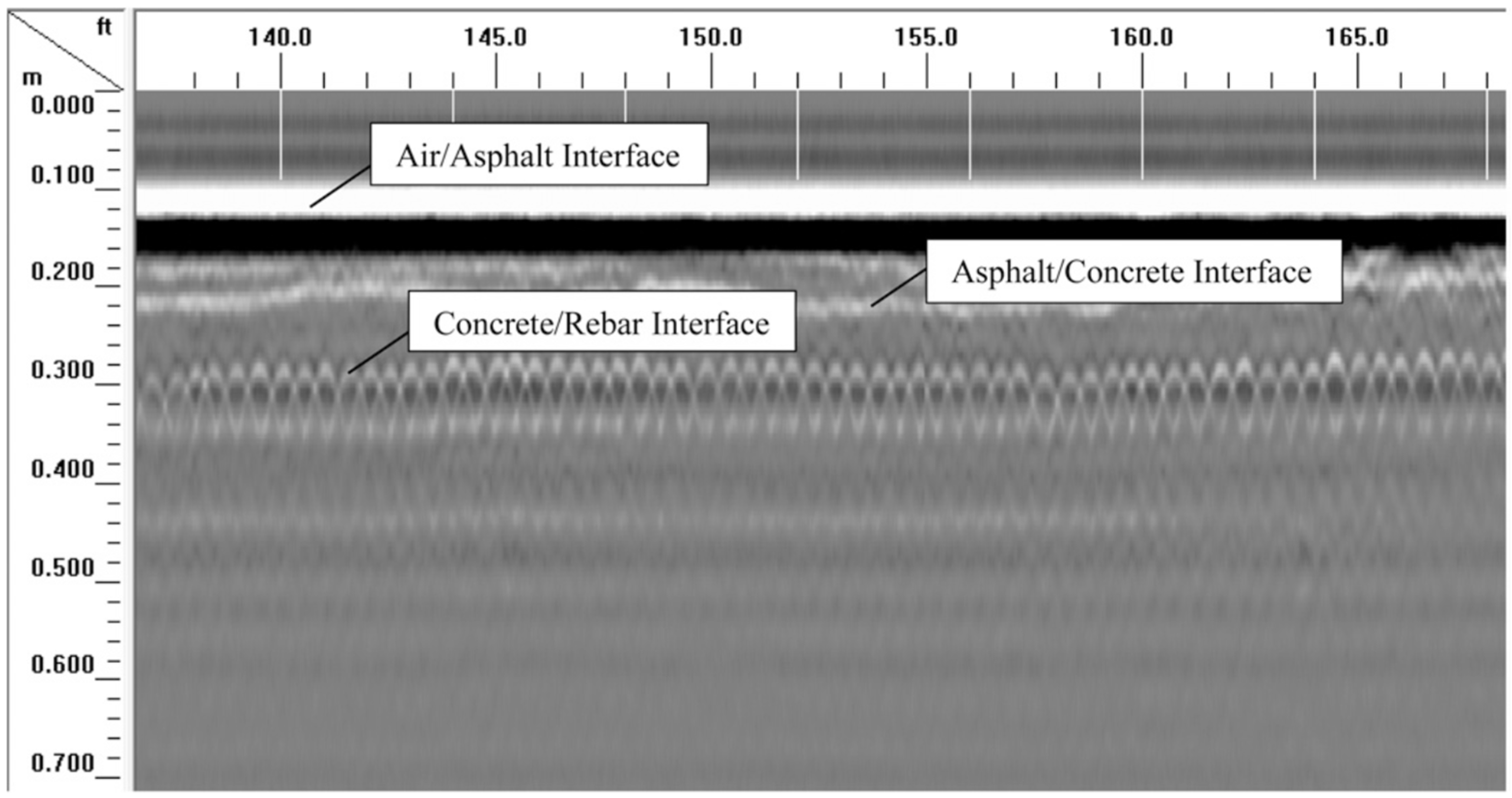
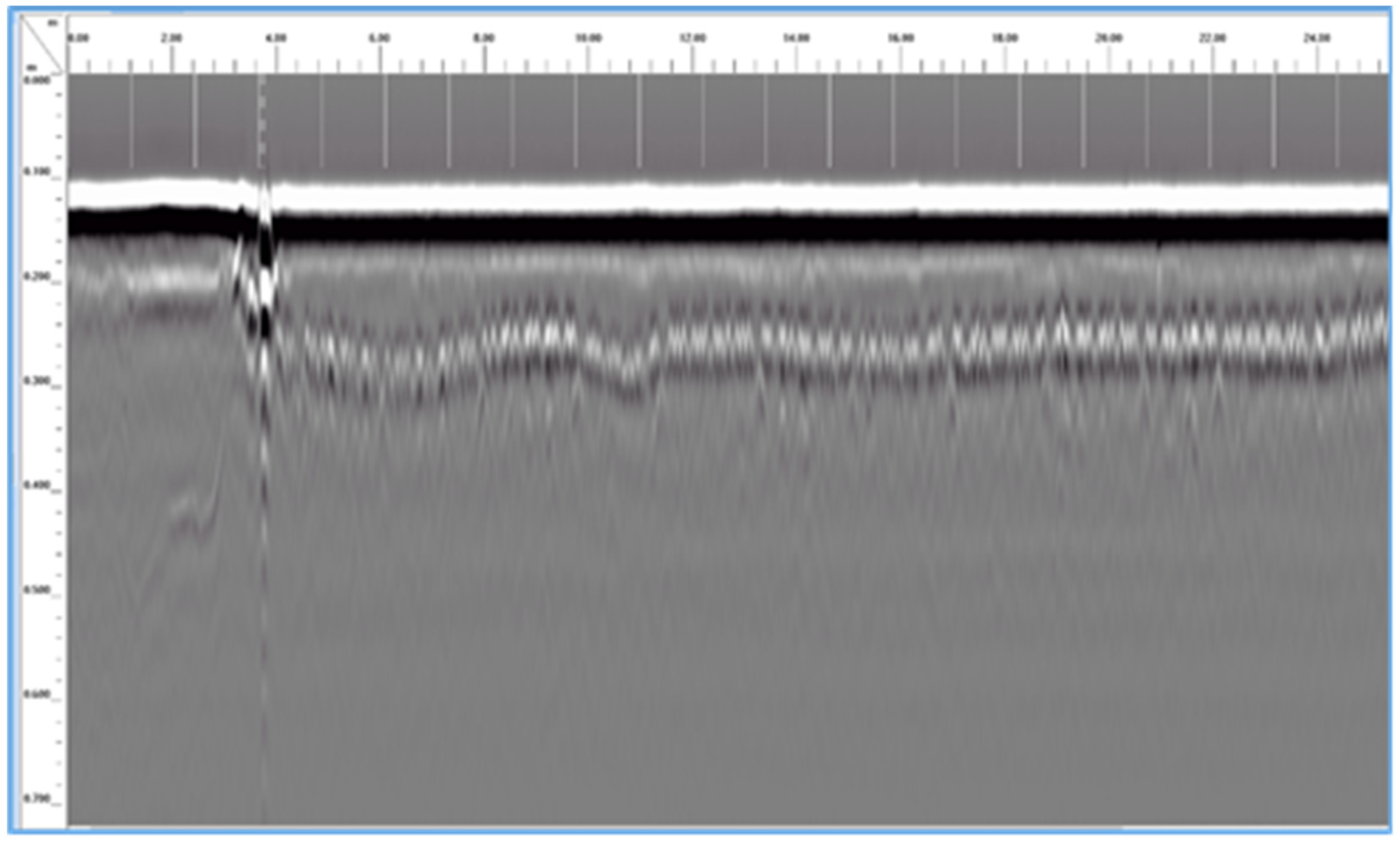
4.1. Pre-Process GPR Profiles

The pre-processing steps on raw GPR B-scans may need to be performed in the proprietary software of the GPR equipment used for scanning such as RADAN® 7 of GSSI® (Nashua, NH, USA) as described by A. Rahman and Zayed [7]. The algorithm used for hyperbola detections, Viola–Jones, is sensitive to the aspect ratio, i.e., the ratio of the width to the height of boxes containing detected regions. Therefore, the first step involves either horizontally stacking or stretching all the GPR profiles of the element to be inspected, if needed, to maintain an aspect ratio closer to the average calculated value of the trained classifier of 1:1.68. It will significantly enhance the detection rate of hyperbolic regions. This involves the following steps: (a) calculate the aspect ratio of the raw B-scans by randomly taking a few samples with the highest frequency of occurrence, and (b) if required, horizontally stack, or stretch profiles by an integer which makes it closer to classifier aspect ratio. For example, Figure 4 shows a sample GPR profile of a large bridge deck whose hyperbolas are stacked very closely to each other and must be horizontally stretched.
The second consecutive step of pre-processing is to increase “display” or “range” gain, if required, to improve the contrast of the GPR B-scans. It would be needed either because of horizontal stretching in the previous step and/or if the contrast were inherently too low in the raw GPR data. The gain applied is optimal yet subjective; however, it is easier to adjust visually by an analyst manually. It should neither be too low nor too high in order to avoid the poor performance of the detection algorithm. The final step is background removal of signals in the B-scans which reduces the high contrast of reflections from asphalt/concrete and/or concrete/air level. This would also improve the contrast of hyperbolic regions in the B-scans. Figure 5 shows the result of a pre-processed sub-section of the sample GPR profile in Figure 4. Firstly, it was horizontally stretched by a factor of “8” to maintain an aspect ratio of 1:1.49; secondly, the display gain was set to “20” in RADAN®; and lastly, the background was removed to distinctly identify the top layer in assisting detections. It is extremely crucial to apply the same pre-processing steps for each of the B-scans of the scanning element to avoid generating unreliable maps. Although these steps could be automated by exporting raw profiles and executing with image processing techniques using a tool such as MATLAB® R2019b the authors of this paper found that for given cases, pre-processing performed using the proprietary software yielded better results in comparison. The application time of these steps is typically just a few minutes, but they would vastly reduce the limitation of using a template-matching approach through improved detection of hyperbolas.

4.2. Hyperbola Detections

After pre-processing the GPR profiles, they are converted into image files (.jpeg, .tiff, etc.) and further processed in MATLAB® environment. The next step is to apply a trained custom classifier for hyperbolic detections in GPR profiles as developed by A. Rahman and Zayed [7]. A brief overview of the Viola–Jones Algorithm along with the data used for training the classifier is discussed. The algorithm was originally introduced as a face-detection framework with the ability to rapidly process images with high detection rates [58]. The complete analysis, development, and application of this algorithm for face detection has been explained by Viola and Jones, 2004 [58], Wang, 2014 [59], and Chaudhari et al., 2015 [60]. It initially utilized “Haar-like” features to detect faces but was later extended to train and detect any object or facial feature using Local Binary Pattern (LBP) [61] and Histogram of Oriented Gradients (HOG) [62] feature types including “Haar”. It has the highest precision and recall rate among popular face-detection algorithms [63]. This algorithm was adopted to detect hyperbolic features in GPR profiles [7] because of following advantages: (a) it is scale-invariant, i.e., it can detect hyperbolas of varying sizes but with similar aspect ratio, (b) it considers the features to be in a full-view upfront position typical of hyperbolas in B-scans, and (c) it has high speed and accuracy with low false-detection rate [64].
The first step is to train the custom classifier using a cascade object detector in MATLAB®. A set of positive samples (image boxes with hyperbolas present) and negative samples (image boxes with non-hyperbolas in GPR profiles) need to be provided and trained through multiple stages. HOG feature type was used as it is suitable to detect objects without fine-scaled details such as cars and people akin to hyperbolas. During the training, negative samples are discarded in each stage and positive samples are processed to the next stage while improving each stage through the boosting technique. Since the classifier is trained to classify only the hyperbolic regions from the background of a GPR profile, i.e., a case of binary categorization, the type of boosting algorithm preferred in literature for this purpose is known as Adaboost [65]. It combines several weak learners by taking a weighted average of decisions in each stage to form a strong classifier, as described in detail by Viola and Jones, 2004 [58]. The detected objects can be classified into the following three categories: (a) true positive: a positive sample identified correctly; (b) false positive: a negative sample mistakenly identified as positive; and (c) false negative: a positive sample mistakenly identified as negative. Figure 6 shows a sample GPR profile with true positives marked in filled yellow boxes while a false negative and a false positive are marked in a surrounding blue box. Besides the number of stages, two other parameters need to be specified for cascade training as follows: (a) the false positive rate—the ratio of total false positives to the summation of all false positives and true negatives; and (b) true positive rate—the ratio of total true positives to the summation all false negatives and true positives.
The data used for training the classifier were taken from a bridge deck, labeled O2, which was inspected as part of comprehensive bridge deck deterioration mapping of nine bridges in the state of Iowa, US [66]. This deck, O2, was specifically chosen as it has small-corroded zones spread across the bridge deck. It carries national highway #93 and is located over a small natural stream in Sumner, Iowa. It has a total span of 63 ft with a clear span length of approximately 60 ft. It has a total width of 48 ft with two-lane roadways besides two 5-foot sidewalks. It was scanned using GSSI® radar equipment named SIR® 3000 (Nashua, NH, USA) with a 1.5 GHz antenna. A grid pattern was laid out and a total of 24 swabs were taken 2 feet apart each to cover the whole width. The training was performed in two consecutive stages with the cascade object detector. Firstly, samples were taken only from one B-scan (first swab): a total of 167 positive samples (hyperbola enclosed boxes) and negative samples (profile with hyperbola removed) were supplied for training. The following were the input parameters: number of cascade stages—20; per-stage false alarm rate—0.5; and per-stage true positive rate—0.995. Subsequently, the obtained classifier which was trained using one profile was used to detect hyperbolas in all 24 profiles. The results obtained when compared to the ground-truth number of hyperbolas (manually counted to be 3843) were as follows: true positives—3400 (88.5%), false positives—14 (0.4%), and false negatives—443(11.5%) [7]. Finally, all these true positives and false negatives were supplied again as input for further training of the classifier using the same input parameters. The resulting custom classifier could be used for detecting hyperbolas in GPR profile scans of any RC structural or bridge element, assuming the profiles were pre-processed as described earlier.
While the custom classifier can majorly detect hyperbolas in B-scans, a few false detections would typically occur in practice. These false positives and false negatives, as shown in Figure 6 for instance, can be eliminated based on regional comparison and statistical analysis through automation [7]. The basic assumption is that the reinforcement bars are stacked in a single or double layer with uniform spacing, generally in the case of RC bridge elements, slabs, or parking lots. The false positives and false negatives could be resolved by applying these three principles in sequential order:
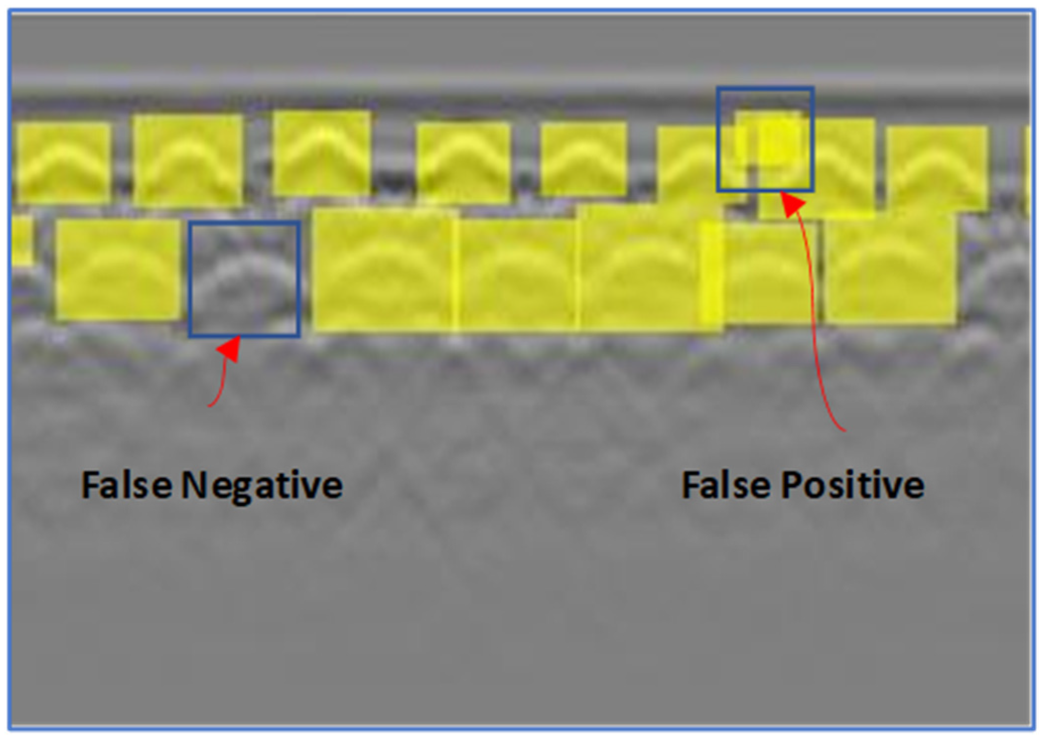
  • The detections (true or false) which do not lie across the top layer and bottom layer (if present) are considered as false positives and eliminated due to their regional position in the B-Scan. The developed code [7] automatically identifies the top layer, but in some cases it yields erroneous results due to complex hyperbolic signatures and/or heavily disoriented top layer in GPR profiles. Therefore, the proposed model utilizes a user-interactive approach to prompt the user to verify if the necessary layer has been identified correctly. In case of incorrect detection, the user is prompted again to roughly mark the top and bottom limit of the top layer present in the GPR profile. Identification of top layer is extremely crucial in generating reliable maps, and thus, a user-interactive approach has been adopted in this step.
  • The actual false positives among overlapping detections are identified and subsequently eliminated along the top/bottom layers by comparing them with the average size and location of neighboring non-overlapping true positives automatically.
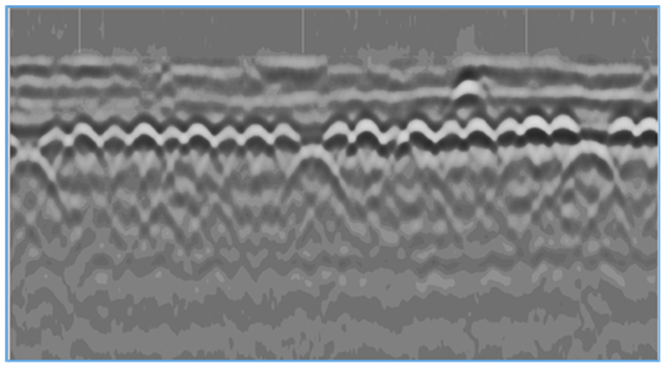
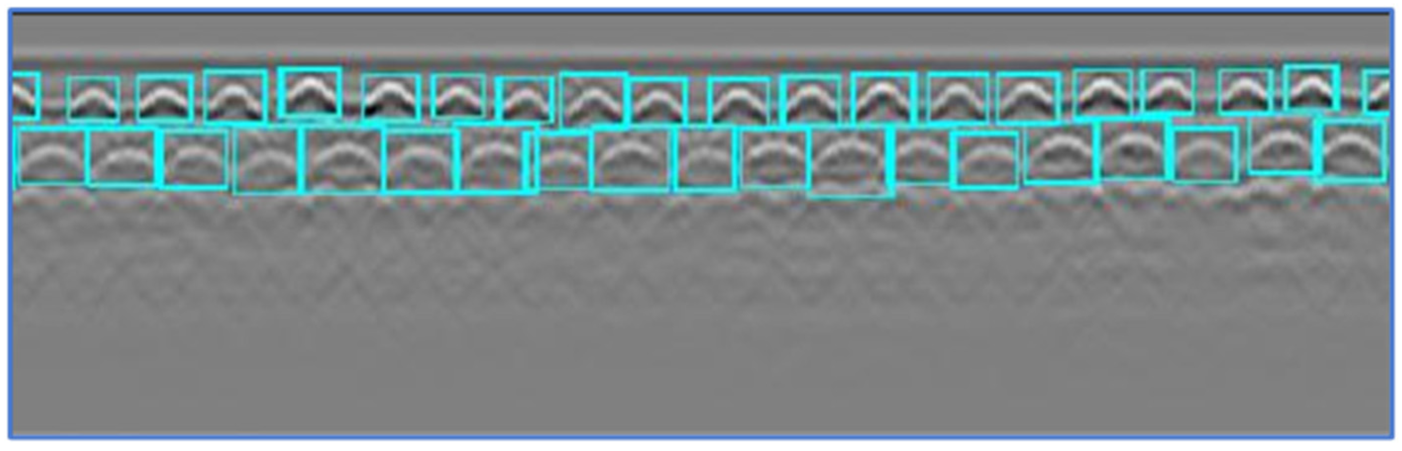
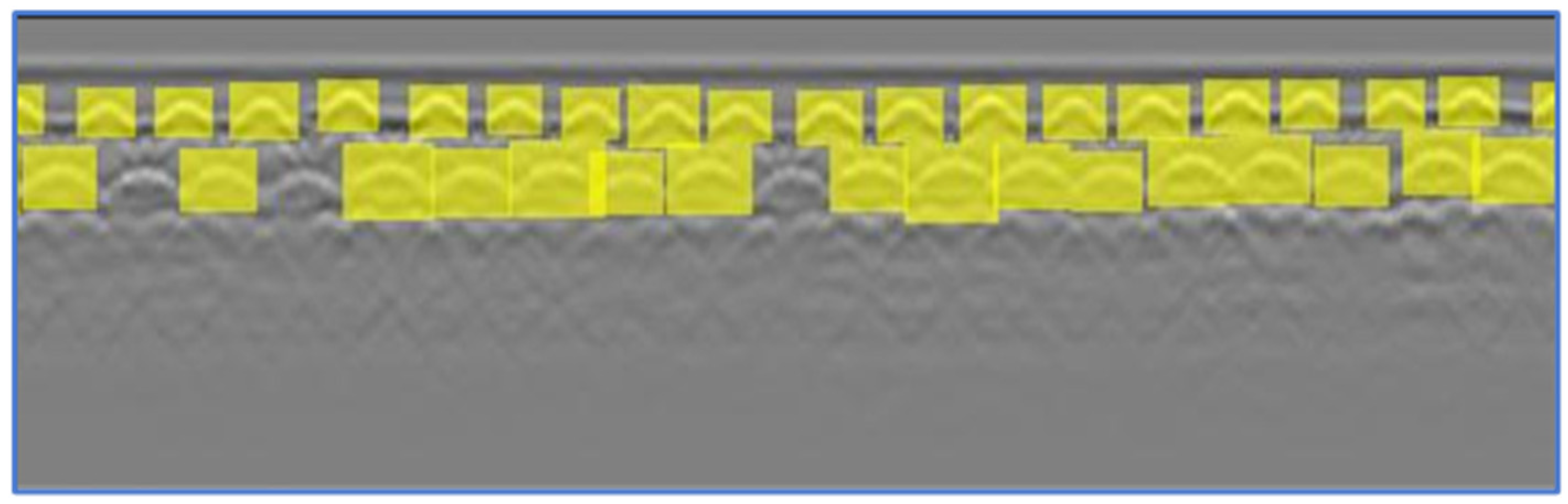
  • The missing gaps present across the top/bottom layers could be either of the following: (a) false negatives, (b) zones with highly distorted hyperbolas or (c) zones with no hyperbolas; probably undetected due to deterioration. These are bounded by rectangular boxes automatically to align with the neighboring true positive detections. Figure 7 shows a cut-out from a GPR profile with three missing detections or gaps after applying a custom classifier. Figure 8 shows the same sample after filling missing gaps in rectangular boxes across both layers. The detections of the GPR profiles are complete and ready for the next step of evaluating textural factors after bounding the top layer and bottom layer (if present) with rectangular boxes composing of true positive detections and missing gaps which include false negatives.

4.3. Deterioration Mapping

After detecting regions in the top (and bottom) layer, a numeric value needs to be assigned to each of these regions or boxes which could correspond to its deterioration level. As discussed earlier for visual-IBA [5], an analyst well-versed in reading GPR profiles marks attenuated areas using his perception and visual judgment. An equivalent factor to distinguish the features in a GPR profile would be texture. Although the human visual system is remarkable in its ability to identify and segment different textures, automating it using computer vision is not easy [67]. Texture refers to both the tactile nature, i.e., tangible “feel” of a surface, and optical nature, i.e., shape or contents in an image [68]. Tamura et al., 1978 [69] refers to six mathematical measures which could relate textural features to visual perception: coarseness, contrast, directionality, line-likeness, regularity, and roughness. In image processing, the texture provides information about the spatial arrangement of intensities in a grey-scale image [70]. A textural factor has been preferred in this model for analyzing detected regions as it can distinguish nuances in patterns of GPR images whereas traditional intensity-based thresholding techniques would be ineffective.
While there are various classifications for analyzing textures, the two main approaches are structural and statistical [70]. A structural approach is utilized for assessing fairly regular or repeated textures such as a brick wall. A statistical approach is preferred for analyzing GPR profiles as these are based on quantitative measurement of intensity arrangements within a region. Entropy, one such statistical factor, has been used in this model as it is a measure of variability or randomness of an image [71]. Essentially, two similar detected regions would have closer entropy values while two dissimilar regions would have a large difference in their entropy values. Corollary, entropy can distinguish areas of deterioration from good to bad based on its values. Higher values of entropy are indicative of relatively better condition of concrete and vice versa. Entropy has no units, and it can be evaluated mathematically directly from the gray level pixels of a region or image as follows [71]: If z is a random variable representing intensity, let p(zi) refer to its respective histogram; wherein, i = 0, 1, 2, 3, …, L−1; L is the number of distinct intensity levels (for example, 256 levels in a gray-scale 8-bit image).
Entropy   = i   = 0 L 1 p ( z i )   log 2 p ( z i )
Entropy is calculated for all the regions detected across a single layer (typically, at the top reinforcement level) for all GPR profiles of the structural element. Subsequently, these values are graded into zones using data-clustering techniques (unsupervised learning). Data classification or supervised learning is not preferred as each set of scanned GPR profiles has unique variations in its data or entropy values corresponding to what constitutes a good or bad region. A broadly agreed framework to classify data-clustering approaches are as follows: (a) hierarchical clustering wherein data is divided through multiple sequences, ranging from a single cluster comprising all individuals to n clusters comprising each individual, and (b) partitional clustering wherein data are divided into prespecified zones in a single step with no hierarchical structure [72]. The number of zones or clusters is usually predetermined in generating deteriorating maps, and therefore a partitional clustering approach has been adopted. K-means is a widely popular data-partitioning algorithm still in use since its development 50 years ago [73]. The entropy values of detected regions are clustered using this algorithm as the maps generated using K-means show good correspondence with existing approaches. The application of this algorithm is demonstrated in the next section with the help of a case study. A set of data can be partitioned using K-means as follows [73]:
If X = {xi}, i = 1, 2, …, n; wherein, X is a set of n data points to be clustered into a set of K-partitions, C = {ck, k = 1, 2, …, K}. C is a set wherein ck is a set of data points of k-th cluster and let µk be its mean. K-means algorithm partitions the data set such that the squared error between the points in each cluster and its mean are minimized. The squared error between ck and µk is calculated as:
J ( c k ) = x i ε c k   | | x i µ k | |
Thus, K-means aims to minimize the sum of this squared error over all K-clusters.
J ( C ) = k = 1 K x i ε c k   | | x i µ k | | 2
The iterative steps of this algorithm can be summarized as [74]:
  • Initially, assign K-partitions randomly or based on some prior information. The centroid means matrix can be written as: M = {µk, k = 1, 2, …, K};
  • Each data point in the data set X is assigned to its nearest clusters cω such that: x i ε   c ω ; | | x i µ ω | | < | | x i µ k | | ; i = 1, 2, …, n; i ω ; k = 1, 2, …, K;
  • The centroid matrix M is recalculated based on the current partition set, C;
  • Repeat steps 2–3 until no change is observed in each cluster.
All the entropy values of detected regions in GPR profiles of a scanned element are clustered with a pre-set number of clusters or zones, typically three or four zones for deterioration mapping. As entropy values are directly correlated to concrete level deterioration, zones with higher values of entropy would correspond to better conditions of concrete and vice versa. A color code is used in generating the map to correspond each detected region with the level of deterioration. The color convention for three zones with respect to concrete condition levels are as follows: green color is good (detected regions zoned with highest values of entropies using K-means), the yellow color is moderate, and the red color is bad (detected regions zoned with lowest values of entropies). If four color zones are used, the following is the convention used in this model: blue is very good, green is good, yellow is moderate, and red is bad. After evaluating the clustered zone of each detection, the first step for mapping is to develop a deterioration scale for each profile. This scale is showcased in Figure 9 using a sample GPR profile. The profile is marked with detected regions in red boxes with evaluated entropy values written, respectively, within them. Each of these boxes is assigned a clustered zone and is represented using a colored deterioration scale as shown on top of the profile. It has only one green and one red region while all others are yellow. If the profile is looked at individually, the yellow zones could be marked as green by an analyst based on visual-image analysis. However, it has been zoned accurately as this method marks these regions not based on entropy values of this individual profile but based on all GPR profiles pertinent to the obtained sample profile. Moreover, the results would be consistently robust as the zoning assignment is not manual. Thus, cases prone to human errors, especially cases with large profiles, are avoided using this developed model. Finally, the deterioration scale developed for each individual profile is staked together for all profiles of the scanned element being inspected to generate a deterioration map. The application of this model with deteriorating mapping and its comparison is discussed in the following section using a case study.

5. Case Study

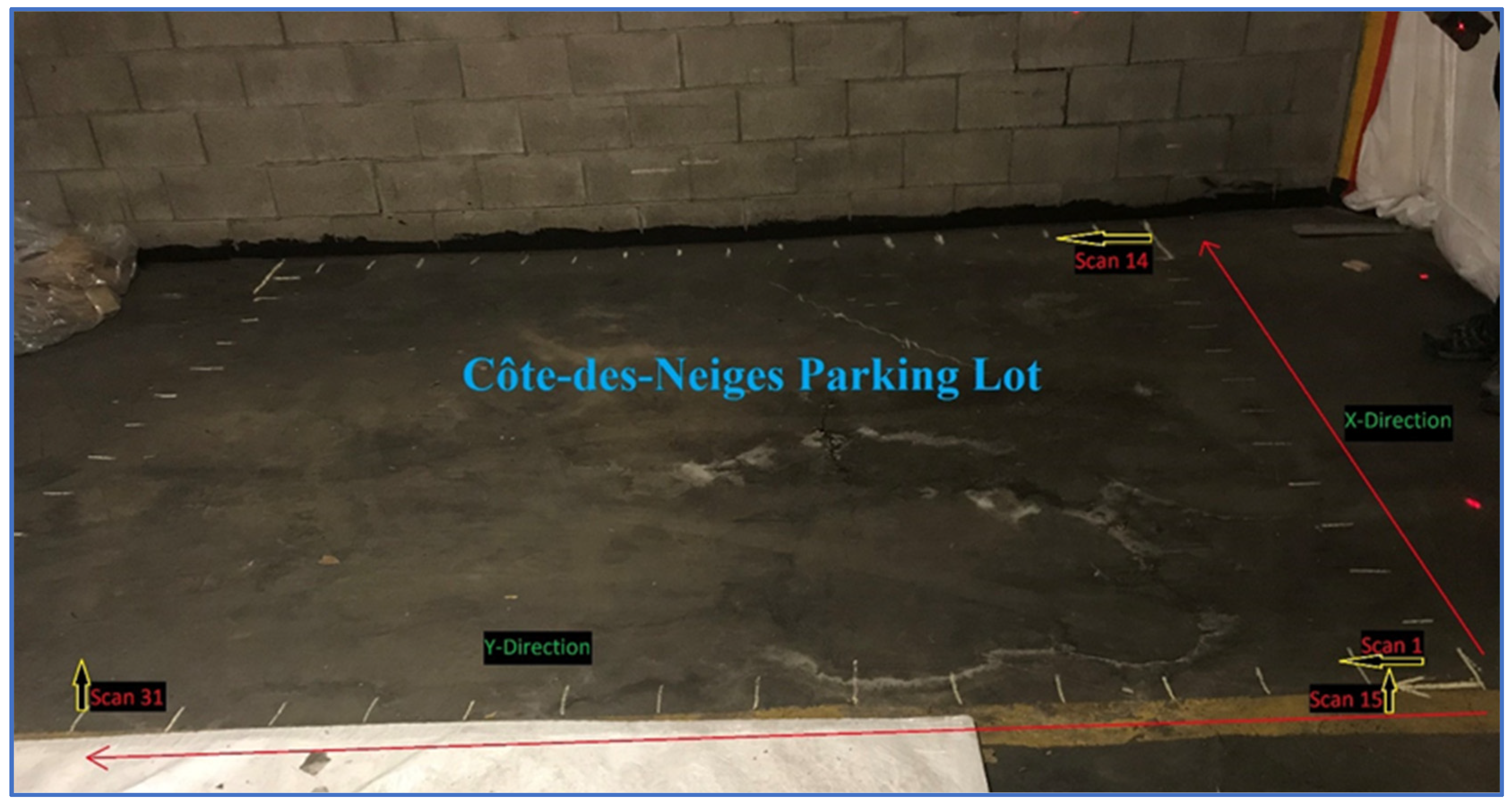
5.1. Data Collection

The implementation of the developed model is demonstrated by a small case study conducted on a concrete slab of a parking lot located in Côte-des-Neiges, Montreal. The scanning was performed across both directions of the slab surface using a hand-held GPR device from GSSI® with an antenna frequency of 1.6 GHz, depth range of 55 cm, an assigned dielectric constant of 6.0 (concrete), and other factors to ensure proper collection of data. The scanned dimensions of the slab were 3.5 m × 2.9 m (approximately). Figure 10 shows the parking lot with the scanning grid pattern shown in white chalk each 20 cm apart (traverse spacing). The figure also indicates the sequence of the 31 swabs taken across both directions: initially, 14 scans were taken along X-direction, as indicated, to cover the longitudinal direction (3.5 m) of the slab, and subsequently, 17 scans were taken along Y-direction to cover the transverse direction (2.9 m).

5.2. Data Processing

The B-scans obtained from the scans were pre-processed in RADAN® software: only the background subtraction was performed as the original scans had aspect ratios relatively closer (1:1.44) to the trained classifier and the range gain was not needed. These scans were subsequently converted into image files and processed in a MATLAB® environment. The hyperbola detections were identified using the cascade detector and the remaining missing detections were enclosed in boxes across the top layer of reinforcement while eliminating false detections based on statistical analysis. After evaluating entropy values of each detected region, a deterioration scale was developed for each scan. Figure 9 mentioned earlier shows the deterioration scale of scan number 6 along the Y-direction for theww cluster zones (green, yellow, red). Finally, separate deterioration maps were created across both X and Y directions while clustering with two color-coded conventions (three and four zones). A comparison of generated maps was made with maps of two existing approaches. The first approach utilized the commonly adopted numerical amplitude method described in ASTM D6087 [4] while the second approach was visual-IBA. Although the amplitude-based approaches are not completely reliable, it can be inferred that there is good correspondence of general concrete condition zones when compared with visual-IBA especially in cases of relatively ideal GPR profiles with no anomalies [5], [29]. The maps based on developed model would have much better correspondence with maps based on visual-IBA as it aims to automate the latter method. Additionally, extreme care was taken by the analyst in marking attenuated areas based on visual-IBA to avoid human errors as much as possible.

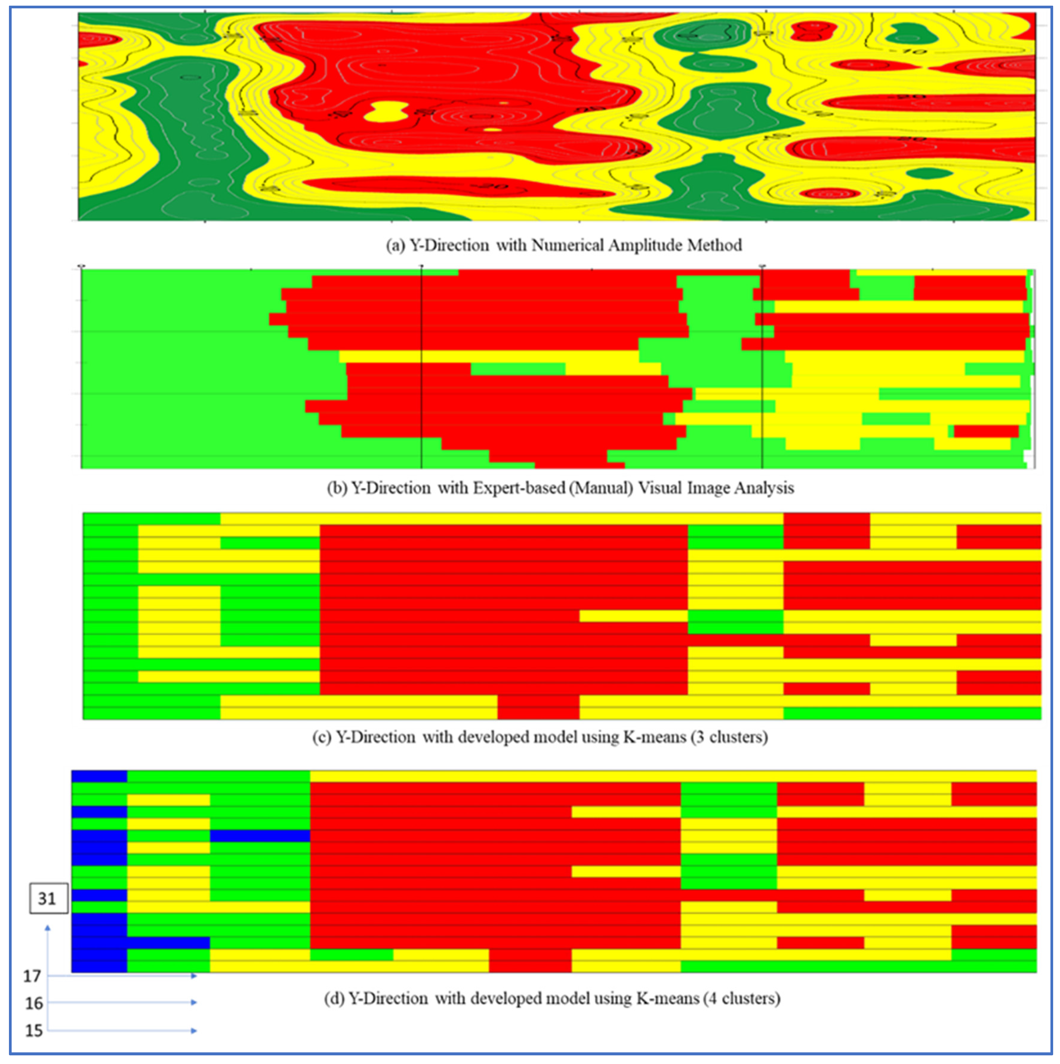
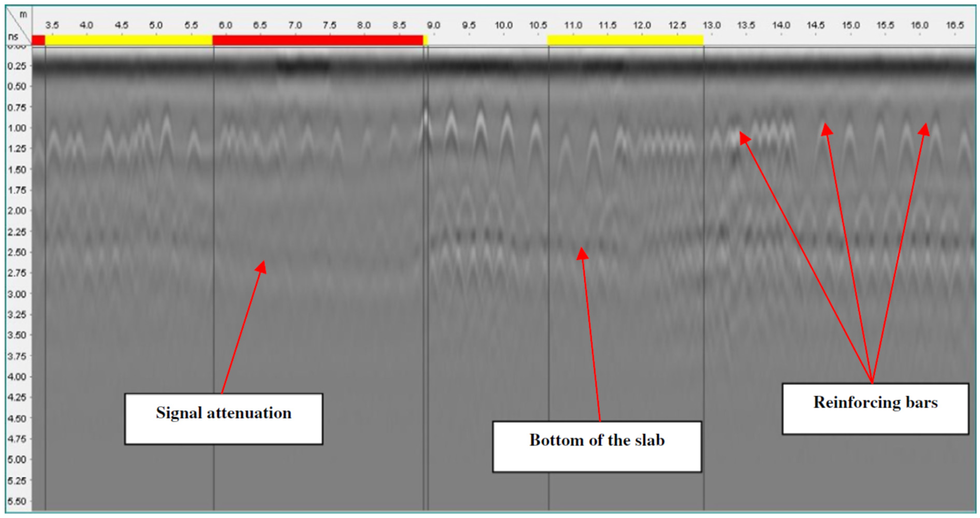
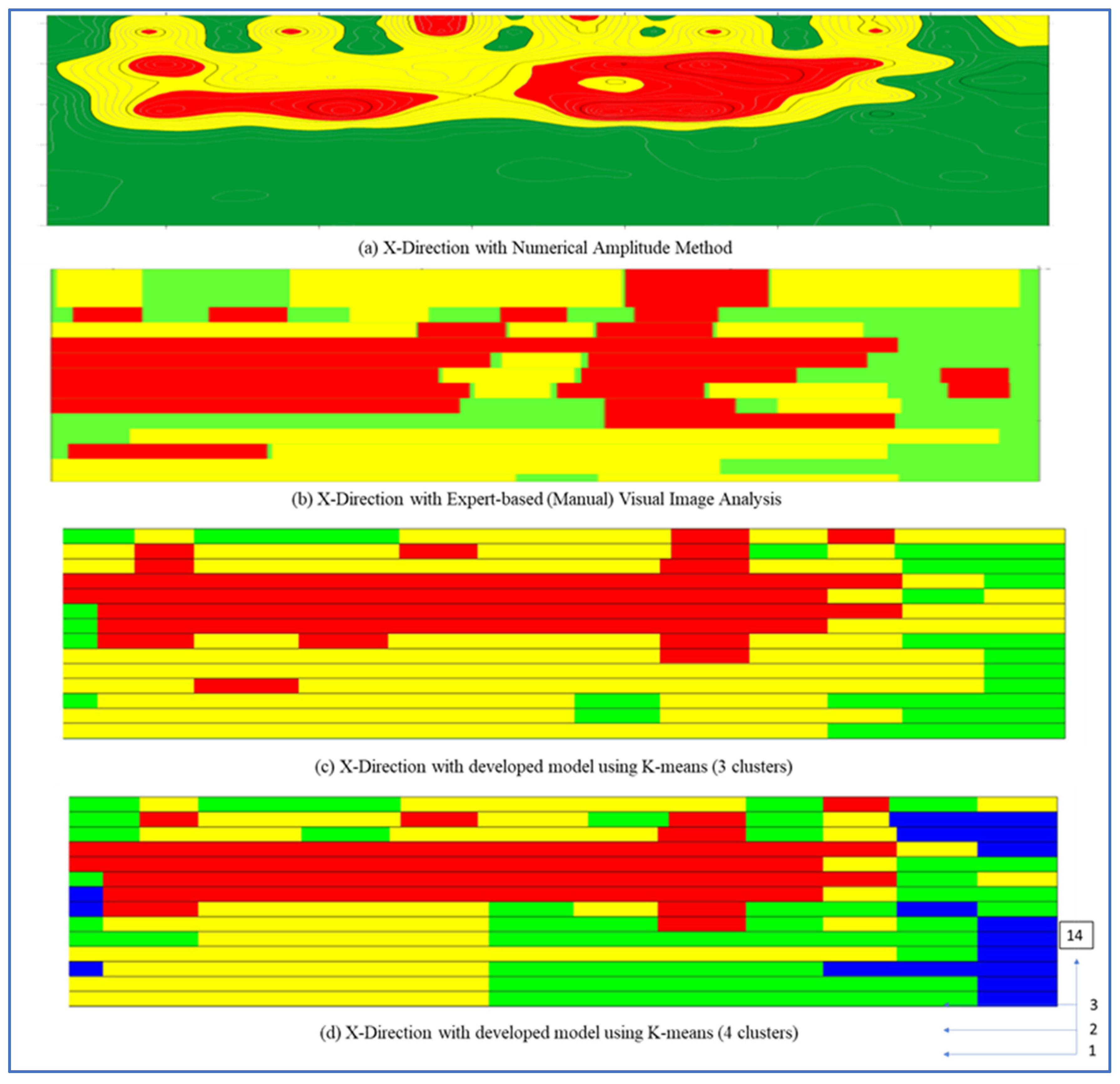
5.3. Results and Their Discussion

The deterioration maps generated along the X and Y direction are represented graphically with a figure and the comparison between varying methods along each direction is discussed separately.
X-direction: Figure 11 shows the four deterioration maps of swabs 1–14 generated along the X-direction using the following methods: (a) amplitude-based method, (b) visual-IBA, (c) developed model with three clusters (green, yellow, red), and (d) developed model with four clusters (blue, green, yellow, red). Table 1 shows the range of entropy values for each zone in maps (c) and (d) and it varies from 7.21 to 4.27 in both. When four cluster zones are utilized, the added blue zone (very good) and green (good) zone majorly occupy the green zone (good) of the three-cluster-based map, while the moderate and severely deteriorated zones remained relatively the same. Table 2 shows a quantitative comparison, i.e., the percentages of green, yellow, and red zones were evaluated for maps based on amplitude, visual-IBA and developed model (three zones only) as these three maps indicate equal number of concrete condition zones (good, moderate, and bad). Firstly, there is some resemblance between the map based on amplitude (map-a) and developed model (map-c) as the upper region is either severely or moderately corroded in both. However, map-c shows that the slab is heavily corroded unlike map-a as the bottom of map-c is also moderately corroded. Moreover, map-c has a total of 84.3% area covered in yellow and red zones when compared to 40.7% in map-a. Map-a estimates (59.6%) that the concrete condition of the slab is four times as good as map-c (15.7%). Secondly, the map based on visual-IBA (map-b) shows greater resemblance to map-c as all the corrosion zones’ distributions are visually similar and that the slab is heavily corroded in the middle region. Additionally, total percentage of corroded concrete (yellow and red) in map-b (77.9%) is close to map-c (84.3%). However, map-b (33.4%) estimates that the slab is slightly more corroded than map-c (29.6%).
Y-direction: Figure 12 shows the four deterioration maps of swabs 15–31 generated along the Y-direction using the aforementioned methods. Table 1 also delineates the range of entropy values for each zone in map-c and map-d varying from 20.86 to 2.22 in both directions. The spread of entropy values is higher along the Y-direction when compared to X; however, these ranges cannot be standardized for each zone as the survey data are unique for any scanned element. There is some visual resemblance between map-c and map-a as the middle region of the slab is heavily corroded along with moderate-to-severe corrosion on the right-side of both maps. Furthermore, in map-c (81.3%) the percentage of total corroded concrete (yellow and red) is closer to that of map-a (77.4%). While there is greater visual resemblance of map-b with map-c in the center and right side of the slab, the left side of map-c displayed some regions of moderate corrosion in the slab unlike map-b. The analyst generating map-b could not identify this disparity as the profiles are looked at individually, unlike in the developed model, which clusters all profiles together and thus is able to distinguish zones more appropriately. Map-c (81.3%) shows that the slab is relatively more corroded than map-b (53.6%). Furthermore, map-b (46.1%) estimates that the slab is in approximately 2.5 times better (good) condition than map-c (18.2%). If we compare results along both directions, it can be inferred that the slab is heavily corroded (~80%) and that map-c is able to estimate the condition of slab more accurately along both directions.
In brief, greater correlation of maps based on an automated approach with visual-IBA method indicates that the developed model potentially identifies the zones of deterioration accurately as the visual-IBA method itself has been proved to be closer to the ground-truth condition [5,29,30]. Moreover, the results are easily reproducible and do not vary due to scientific analysis. However, for superior validation of the developed model, the maps generated must be compared with lab tests and in situ destructive techniques in the field. Finally, identification of deteriorated zones using the developed model can help structural inspectors to locally identify deteriorated zones within a structural element that require immediate attention for repair and rehabilitation. Such maps could also be useful in modelling a deteriorated structure to assess the remaining capacity of the structure [75].

6. Conclusions and Future Work

A model has been developed to generate reliable deterioration maps using GPR B-scans for RC bridge and structural elements. The proposed method is superior to existing amplitude-based methods and aims to reduce the subjectivity of visual-IBA through automation. The following inferences can be drawn based on the developed methodology and demonstrated case study:
  • Pre-processing of GPR profiles is necessary to improve the detection rate of hyperbolas, especially maintaining an aspect ratio closer to the trained classifier.
  • Most hyperbolas are detected in B-scans based on a classifier trained on a complete real bridge-deck data using Viola–Jones Algorithm. The remaining missing hyperbolas and regions are enclosed in boxes across the top/bottom layer of reinforcement automatically with a user-interactive approach based on regional comparison and statistical analysis.
  • A statistical textural factor, entropy, has been evaluated to differentiate detected regions closely equivalent to the human visual system.
  • The entropy values are clustered into three or four zones using K-means clustering. A deterioration scale is developed for all B-scans by assigning a color code to each of the detected regions relative to the zone in which they were clustered. These scales are subsequently stacked together to generate a deterioration map.
  • A comparison of the deterioration map of a parking lot case study shows considerable correspondence of the developed model with existing approaches, especially with the visual image-based analysis.
The developed model has few limitations of its own which the authors wish to address as part of the ongoing research project. Firstly, the model does not consider various anomalies which include (a) structural anomalies such as presence of a structural member across the top layer such as a beam/column, voids (air or water), variation in reinforcement bar spacing, staggered rebars, chloride saturation; and (b) surface anomalies such as pavement debonding, expansion joints, concrete cut-and-repair. Secondly, validation of deterioration zones must be performed with in situ destructive techniques on existing structures and in a controlled laboratory environment. Lastly, the detection rate may not be accurate in GPR profiles with very ill-shaped hyperbolas in complex media. The authors aim to address these drawbacks by improving the developed model in the future by incorporating the following: (a) the anomalies would be automatically detected and considered while developing the deterioration scale, (b) more accurate validation would be achieved by testing samples with varying degrees of deterioration in a laboratory and through in situ tests such as visual inspection, HCP or core-sampling (destructive tests), and (c) improving the hyperbola detection model. However, the model in its current state does generate reliable maps for most elements scanned, with GPR having no anomalies across the inspected layer (top/bottom) of reinforcement. The ongoing work including the developed model seeks to develop a robust tool for condition assessment that can be readily utilized by transportation authorities for bridge maintenance and repair.

Author Contributions

Conceptualization, methodology, M.A.R., A.B. and T.Z.; writing—original draft preparation, M.A.R. and A.B.; formal analysis, data curation, M.A.R.; validation, writing—review and editing, M.A.R., A.B. and T.Z.; supervision, A.B. and T.Z.; funding acquisition, A.B. All authors have read and agreed to the published version of the manuscript.

Funding

This research was funded and supported by the Ministère des Transports du Québec (No. R730.2).

Institutional Review Board Statement

Not applicable.

Informed Consent Statement

Not applicable.

Data Availability Statement

The data presented in this study are available on request from the corresponding author. Some restrictions may apply to the availability of these data as it is shared with the transportation authority of a provisional government.

Acknowledgments

The authors of this paper wish to thank Concordia University for providing its research facilities and other services.

Conflicts of Interest

The authors of this work hereby declare that this work is originally performed by them and there are no conflicts of interests with any other parties.

References

  1. Heymsfield, E.; Kuss, M.L. Supplementing Current Visual Highway Bridge Inspections with Gigapixel Technology. J. Perform. Constr. Facil. 2016, 30, 04015015. [Google Scholar] [CrossRef]
  2. Gucunski, N. ; National Research Council. Nondestructive Testing to Identify Concrete Bridge Deck Deterioration; Transportation Research Board: Washington, DC, USA, 2013. [Google Scholar]
  3. Yehia, S.; Abudayyeh, O.; Nabulsi, S.; Abdelqader, I. Detection of Common Defects in Concrete Bridge Decks Using Nondestructive Evaluation Techniques. J. Bridg. Eng. 2007, 12, 215–225. [Google Scholar] [CrossRef]
  4. ASTM D6087; Standard Test Method for Evaluating Asphalt-Covered Concrete Bridge Decks Using Ground Penetrating Radar. American Society for Testing and Materials: West Conshohocken, PA, USA, 2015; p. D6087-08.
  5. Tarussov, A.; Vandry, M.; De La Haza, A. Condition assessment of concrete structures using a new analysis method: Ground-penetrating radar computer-assisted visual interpretation. Constr. Build. Mater. 2013, 38, 1246–1254. [Google Scholar] [CrossRef]
  6. Rahman, M.A.; Zayed, T. Developing Corrosion Maps of RC bridge elements based on automated visual image analysis. In Proceedings of the Session of the 2016 Conference of the Transportation Association of Canada, Toronto, ON, Canada, 22–28 September 2016. [Google Scholar]
  7. Rahman, M.A.; Zayed, T. Viola-Jones Algorithm for Automatic Detection of Hyperbolic Regions in GPR Profiles of Bridge Decks. In Proceedings of the 2018 IEEE Southwest Symposium on Image Analysis and Interpretation (SSIAI), Las Vegas, NV, USA, 8–10 April 2018; pp. 1–4. [Google Scholar] [CrossRef]
  8. Varnavina, A.V.; Khamzin, A.K.; Torgashov, E.V.; Sneed, L.H.; Goodwin, B.T.; Anderson, N.L. Data acquisition and processing parameters for concrete bridge deck condition assessment using ground-coupled ground penetrating radar: Some considerations. J. Appl. Geophys. 2015, 114, 123–133. [Google Scholar] [CrossRef]
  9. Gehrig, M.D.; Morris, D.V.; Bryant, J.T. Ground penetrating radar for concrete evaluation studies. Tech. Present. Pap. Perform. Found. Assoc. 2004, 197–200. [Google Scholar]
  10. Dinh, K.; Zayed, T.; Romero, F.; Tarussov, A. Method for Analyzing Time-Series GPR Data of Concrete Bridge Decks. J. Bridg. Eng. 2015, 20, 04014086. [Google Scholar] [CrossRef]
  11. Clemena, G.G. Nondestructive Inspection of Overlaid Bridge Decks with Ground-Penetrating Radar; Transportation Research Board: Washington, DC, USA, 1983; pp. 21–32, No. 899. [Google Scholar]
  12. Carter, C.R.; Chung, T.; Holt, F.B.; Manning, D.G. An automated signal processing system for the signature analysis of radar waveforms from bridge decks. Can. Electr. Eng. J. 1986, 11, 128–137. [Google Scholar] [CrossRef]
  13. Chung, T.; Carter, C.R.; Reel, R.; Tharmabala, T.; Wood, D. Impulse radar signatures of selected bridge deck structures. In Proceedings of the Canadian Conference on Electrical and Computer Engineering, Vancouver, BC, Canada, 14–17 September 1993; pp. 59–62. [Google Scholar] [CrossRef]
  14. Maser, K.R. New Technology for Bridge Deck Assessment, Phase II Report; Report No FHWA-NETC-90-01; Centre for Transportation Studies, Massachusetts Institute of Technology: Cambridge, MA USA, 1990. [Google Scholar]
  15. Maser, K.; Bernhardt, M. Statewide Bridge Deck Survey using Ground Penetrating Radar. In Proceedings of the Structural Materials Technology IV—An NDT Conference, Atlantic City, NJ, USA, 28 February–3 March 2000. [Google Scholar]
  16. Romero, F.A.; Roberts, G.E.; Roberts, R.L. Evaluation of GPR Bridge Deck Survey Results used for Delineation of Removal/Maintenance Quantity Boundaries on Asphalt-Overlaid, Reinforced Concrete Deck. In Proceedings of the Structural Materials Technology IV—An NDT Conference, Atlantic City, NJ, USA, 28 February–3 March 2000. [Google Scholar]
  17. Barnes, C.L.; Trottier, J.-F. Effectiveness of Ground Penetrating Radar in Predicting Deck Repair Quantities. J. Infrastruct. Syst. 2004, 10, 69–76. [Google Scholar] [CrossRef]
  18. Parrillo, R.; Roberts, R.; Haggan, A. Bridge deck condition assessment using ground penetrating radar. Proc. ECNDT Berlin 2006, 2526, 112. [Google Scholar]
  19. Barnes, C.L.; Trottier, J.-F.; Forgeron, D. Improved concrete bridge deck evaluation using GPR by accounting for signal depth–amplitude effects. NDT E Int. 2008, 41, 427–433. [Google Scholar] [CrossRef]
  20. Dinh, K.; Gucunski, N.; Kim, J.; Duong, T. Method for attenuation assessment of GPR data from concrete bridge decks. NDT E Int. 2017, 92, 50–58. [Google Scholar] [CrossRef]
  21. Sultan, A.A.; Washer, G.A. Reliability Analysis of Ground-Penetrating Radar for the Detection of Subsurface Delamination. J. Bridg. Eng. 2018, 23, 04017131. [Google Scholar] [CrossRef]
  22. Dinh, K.; Gucunski, N.; Zayed, T. Automated visualization of concrete bridge deck condition from GPR data. NDT E Int. 2019, 102, 120–128. [Google Scholar] [CrossRef]
  23. Goulias, D.G.; Cafiso, S.; Di Graziano, A.; Saremi, S.G.; Currao, V. Condition Assessment of Bridge Decks through Ground-Penetrating Radar in Bridge Management Systems. J. Perform. Constr. Facil. 2020, 34, 04020100. [Google Scholar] [CrossRef]
  24. Gagarin, N.; Goulias, D.; Mekemson, J.; Cutts, R.; Andrews, J. Development of Novel Methodology for Assessing Bridge Deck Conditions Using Step Frequency Antenna Array Ground Penetrating Radar. J. Perform. Constr. Facil. 2020, 34, 04019113. [Google Scholar] [CrossRef]
  25. Jiao, L.; Ye, Q.; Cao, X.; Huston, D.; Xia, T. Identifying concrete structure defects in GPR image. Measurement 2020, 160, 107839. [Google Scholar] [CrossRef]
  26. Rhee, J.-Y.; Park, K.-E.; Lee, K.-H.; Kee, S.-H. A Practical Approach to Condition Assessment of Asphalt-Covered Concrete Bridge Decks on Korean Expressways by Dielectric Constant Measurements Using Air-Coupled GPR. Sensors 2020, 20, 2497. [Google Scholar] [CrossRef]
  27. Pashoutani, S.; Zhu, J. Ground Penetrating Radar Data Processing for Concrete Bridge Deck Evaluation. J. Bridg. Eng. 2020, 25, 04020030. [Google Scholar] [CrossRef]
  28. Dinh, K.; Gucunski, N.; Tran, K.; Novo, A.; Nguyen, T. Full-resolution 3D imaging for concrete structures with dual-polarization GPR. Autom. Constr. 2021, 125, 103652. [Google Scholar] [CrossRef]
  29. Abouhamad, M.; Dawood, T.; Jabri, A.; Alsharqawi, M.; Zayed, T. Corrosiveness mapping of bridge decks using image-based analysis of GPR data. Autom. Constr. 2017, 80, 104–117. [Google Scholar] [CrossRef]
  30. Dawood, T.; Zhu, Z.; Zayed, T. Deterioration mapping in subway infrastructure using sensory data of GPR. Tunn. Undergr. Space Technol. 2020, 103, 103487. [Google Scholar] [CrossRef]
  31. Illingworth, J.; Kittler, J. A survey of the hough transform. Comput. Vision, Graph. Image Process. 1988, 44, 87–116. [Google Scholar] [CrossRef]
  32. Falorni, P.; Capineri, L.; Masotti, L. 3-D radar imaging of buried utilities by features estimation of hyperbolic diffraction patterns in radar scans. Penetrating Radar 2004, 1, 403–406. [Google Scholar]
  33. Windsor, C.; Capineri, L.; Falorni, P.; Matucci, S.; Borgioli, G. The estimation of buried pipe diameters using ground penetrating radar. Insight-Non-Destructive Test. Cond. Monit. 2005, 47, 394–399. [Google Scholar] [CrossRef]
  34. Hui-Lin, Z.; Mao, T.; Xiao-Li, C. Feature extraction and classification of echo signal of ground penetrating radar. Wuhan Univ. J. Nat. Sci. 2005, 10, 1009–1012. [Google Scholar] [CrossRef]
  35. Dell’Acqua, A.; Sarti, A.; Tubaro, S.; Zanzi, L. Detection of linear objects in GPR data. Signal Process. 2004, 84, 785–799. [Google Scholar] [CrossRef]
  36. Liu, Y.; Wang, M.; Cai, Q. The target detection for GPR images based on curve fitting. In Proceedings of the 2010 3rd International Congress on Image and Signal Processing, Yantai, China, 16–18 October 2010; Volume 6, pp. 2876–2879. [Google Scholar]
  37. Mertens, L.; Persico, R.; Matera, L.; Lambot, S. Automated Detection of Reflection Hyperbolas in Complex GPR Images with No A Priori Knowledge on the Medium. IEEE Trans. Geosci. Remote Sens. 2016, 54, 580–596. [Google Scholar] [CrossRef]
  38. Al-Nuaimy, W.; Huang, Y.; Nakhkash, M.; Fang, M.; Nguyen, V.; Eriksen, A. Automatic detection of buried utilities and solid objects with GPR using neural networks and pattern recognition. J. Appl. Geophys. 2000, 43, 157–165. [Google Scholar] [CrossRef]
  39. Gamba, P.; Lossani, S. Neural detection of pipe signatures in ground penetrating radar images. IEEE Trans. Geosci. Remote Sens. 2000, 38, 790–797. [Google Scholar] [CrossRef]
  40. Singh, N.P.; Nene, M.J. Buried object detection and analysis of GPR images: Using neural network and curve fitting. In Proceedings of the 2013 Annual International Conference on Emerging Research Areas and 2013 International Conference on Microelectronics, Communications and Renewable Energy, Kanjirapally, India, 4–6 June 2013; Institute of Electrical and Electronics Engineers (IEEE): New York, NY, USA, 2013; pp. 1–6. [Google Scholar] [CrossRef]
  41. Pham, M.-T.; Lefèvre, S. Buried Object Detection from B-Scan Ground Penetrating Radar Data Using Faster-RCNN. In Proceedings of the IGARSS 2018—2018 IEEE International Geoscience and Remote Sensing Symposium, Valencia, Spain, 22–27 July 2018; pp. 6804–6807. [Google Scholar]
  42. Kaneko, T. Radar image processing for locating underground linear objects. IEICE Trans. Inf. Syst. 1991, 74, 3451–3458. [Google Scholar]
  43. Shihab, S.; Al-Nuaimy, W. Radius Estimation for Cylindrical Objects Detected by Ground Penetrating Radar. Subsurf. Sens. Technol. Appl. 2005, 6, 151–166. [Google Scholar] [CrossRef]
  44. Pasolli, E.; Melgani, F.; Donelli, M. Automatic Analysis of GPR Images: A Pattern-Recognition Approach. IEEE Trans. Geosci. Remote Sens. 2009, 47, 2206–2217. [Google Scholar] [CrossRef]
  45. Delbo, S.; Gamba, P.; Roccato, D. A fuzzy shell clustering approach to recognize hyperbolic signatures in subsurface radar images. IEEE Trans. Geosci. Remote Sens. 2000, 38, 1447–1451. [Google Scholar] [CrossRef]
  46. Harkat, H.; Ruano, A.; Ruano, M.; Bennani, S. Classifier Design by a Multi-Objective Genetic Algorithm Approach for GPR Automatic Target Detection. IFAC-PapersOnLine 2018, 51, 187–192. [Google Scholar] [CrossRef]
  47. Wang, Z.W.; Zhou, M.; Slabaugh, G.; Zhai, J.; Fang, T. Automatic Detection of Bridge Deck Condition From Ground Penetrating Radar Images. IEEE Trans. Autom. Sci. Eng. 2010, 8, 633–640. [Google Scholar] [CrossRef]
  48. Kaur, P.; Dana, K.J.; Romero, F.A.; Gucunski, N. Automated GPR Rebar Analysis for Robotic Bridge Deck Evaluation. IEEE Trans. Cybern. 2016, 46, 2265–2276. [Google Scholar] [CrossRef] [PubMed]
  49. Dou, Q.; Wei, L.; Magee, D.R.; Cohn, A.G. Real-Time Hyperbola Recognition and Fitting in GPR Data. IEEE Trans. Geosci. Remote Sens. 2017, 55, 51–62. [Google Scholar] [CrossRef] [Green Version]
  50. Yuan, C.; Li, S.; Cai, H.; Kamat, V.R. GPR Signature Detection and Decomposition for Mapping Buried Utilities with Complex Spatial Configuration. J. Comput. Civ. Eng. 2018, 32, 04018026. [Google Scholar] [CrossRef]
  51. Dinh, K.; Gucunski, N.; Duong, T.H. An algorithm for automatic localization and detection of rebars from GPR data of concrete bridge decks. Autom. Constr. 2018, 89, 292–298. [Google Scholar] [CrossRef]
  52. Zhou, X.; Chen, H.; Li, J. An Automatic GPR B-Scan Image Interpreting Model. IEEE Trans. Geosci. Remote Sens. 2018, 56, 3398–3412. [Google Scholar] [CrossRef]
  53. Lei, W.; Hou, F.; Xi, J.; Tan, Q.; Xu, M.; Jiang, X.; Liu, G.; Gu, Q. Automatic hyperbola detection and fitting in GPR B-scan image. Autom. Constr. 2019, 106, 102839. [Google Scholar] [CrossRef]
  54. Ozkaya, U.; Melgani, F.; Bejiga, M.B.; Seyfi, L.; Donelli, M. GPR B scan image analysis with deep learning methods. Measurement 2020, 165, 107770. [Google Scholar] [CrossRef]
  55. Asadi, P.; Gindy, M.; Alvarez, M.; Asadi, A. A computer vision based rebar detection chain for automatic processing of concrete bridge deck GPR data. Autom. Constr. 2020, 112, 103106. [Google Scholar] [CrossRef]
  56. Hou, F.; Lei, W.; Li, S.; Xi, J.; Xu, M.; Luo, J. Improved Mask R-CNN with distance guided intersection over union for GPR signature detection and segmentation. Autom. Constr. 2021, 121, 103414. [Google Scholar] [CrossRef]
  57. Utsi, E.C. Ground Penetrating Radar: Theory and Practice; Butterworth-Heinemann: Oxford, UK, 2017. [Google Scholar]
  58. Viola, P.; Jones, M.J. Robust Real-Time Face Detection. Int. J. Comput. Vis. 2004, 57, 137–154. [Google Scholar] [CrossRef]
  59. Wang, Y.-Q. An Analysis of the Viola-Jones Face Detection Algorithm. Image Process. Line 2014, 4, 128–148. [Google Scholar] [CrossRef]
  60. Chaudhari, M.; Sondur, S.; Vanjare, G. A review on Face Detection and study of Viola Jones method. Int. J. Comput. Trends Technol. 2015, 25, 54–61. [Google Scholar] [CrossRef]
  61. Ojala, T.; Pietikainen, M.; Maenpaa, T. Multiresolution gray-scale and rotation invariant texture classification with local binary patterns. IEEE Trans. Pattern Anal. Mach. Intell. 2002, 24, 971–987. [Google Scholar] [CrossRef]
  62. Dalal, N.; Triggs, B. Histograms of Oriented Gradients for Human Detection. In Proceedings of the Computer Vision and Pattern Recognition, San Diego, CA, USA, 20–26 June 2005; pp. 886–893. [Google Scholar]
  63. Dang, K.; Sharma, S. Review and comparison of face detection algorithms. In Proceedings of the 2017 7th International Conference on Cloud Computing, Data Science & Engineering-Confluence, Noida, India, 12–13 January 2017; Institute of Electrical and Electronics Engineers (IEEE): New York, NY, USA, 2017; pp. 629–633. [Google Scholar]
  64. Gupta, M.V.; Sharma, D. A study of various face detection methods. Int. J. Adv. Res. Comput. Commun. Eng. 2014, 3, 6694–6697. [Google Scholar]
  65. Freund, Y.; Schapire, R.E. A Decision-Theoretic Generalization of On-Line Learning and an Application to Boosting. J. Comput. Syst. Sci. 1997, 55, 119–139. [Google Scholar] [CrossRef] [Green Version]
  66. Gucunski, N.; Romero, F.; Kruschwitz, S.; Feldmann, R.; Parvardeh, H. Comprehensive Bridge Deck Deterioration Mapping of nine Bridges by Nondestructive Evaluation Technologies; No. Project SPR-NDEB(90)- 8H-00; Iowa Department of Transportation: IA, USA, 2011.
  67. Tatu, A.; Bansal, S. A Novel Active Contour Model for Texture Segmentation BT—Energy Minimization Methods in Computer Vision and Pattern Recognition; Springer: Cham, Switzerland, 2015; pp. 223–236. [Google Scholar]
  68. Manjunath, B.S.; Ma, W.Y. Texture features for browsing and retrieval of image data. IEEE Trans. Pattern Anal. Mach. Intell. 1996, 18, 837–842. [Google Scholar] [CrossRef] [Green Version]
  69. Tamura, H.; Mori, S.; Yamawaki, T. Textural Features Corresponding to Visual Perception. IEEE Trans. Syst. Man Cybern. 1978, 8, 460–473. [Google Scholar] [CrossRef]
  70. Shapiro, L.G.; Stockman, G.C. Computer Vision; Prentice Hall: Hoboken, NJ, USA, 2001. [Google Scholar]
  71. Gonzalez, R.; Woods, R.; Eddins, S. Digital Image Processing Using MATLAB®; Tata McGraw Hill Education: New York, NY, USA, 2010. [Google Scholar]
  72. Everitt, B.; Landau, S.; Leese, M. Cluster Analysis. In A Hodder Arnold Publication; Willey: London, UK, 2001. [Google Scholar]
  73. Jain, A.K. Data clustering: 50 years beyond K-means. Pattern Recognit. Lett. 2010, 31, 651–666. [Google Scholar] [CrossRef]
  74. Xu, R.; Wunsch, D. Survey of Clustering Algorithms. IEEE Trans. Neural Netw. 2005, 16, 645–678. [Google Scholar] [CrossRef] [Green Version]
  75. Ghodoosi, F.; Bagchi, A.; Zayed, T.; Hosseini, M.R. Method for developing and updating deterioration models for concrete bridge decks using GPR data. Autom. Constr. 2018, 91, 133–141. [Google Scholar] [CrossRef]
Figure 1. A GPR B-Scan of a bridge deck with asphalt overlay showing various interfaces and hyperbolic reflections from rebars [10].
Remotesensing 14 01131 g001
Figure 2. Attenuated areas marked in a GPR profile based on Image-Based Analysis [5].
Remotesensing 14 01131 g002
Figure 3. Complete methodology of developed model to generate deterioration maps.
Remotesensing 14 01131 g003
Figure 4. A GPR profile section of a large bride deck with stacked hyperbolas [7].
Remotesensing 14 01131 g004
Figure 5. A sub-section of the GPR profile after applying pre-processing steps including horizontal stretching, range gain and background removal [7].
Remotesensing 14 01131 g005
Figure 6. A sample GPR profile showing true positives and false detections.
Remotesensing 14 01131 g006
Figure 7. A sample cut-out of a GPR profile after applying a custom classifier.
Remotesensing 14 01131 g007
Figure 8. A sample cut-out of a GPR profile after complete detections.
Remotesensing 14 01131 g008
Figure 9. A sample GPR profile with detections in red boxes, entropy values enclosed, and deterioration scale in color on top.
Remotesensing 14 01131 g009
Figure 10. Parking lot scanned using GPR across both directions of the slab surface.
Remotesensing 14 01131 g010
Figure 11. Deterioration maps comparison along X-direction.
Remotesensing 14 01131 g011
Figure 12. Deterioration maps comparison along Y-direction.
Remotesensing 14 01131 g012
Table 1. Range of entropy values in generated deterioration maps.
Map-DirectionZoneColor (Entropy Values)
BlueGreenYellowRed
X-direction3 Clusters-7.21–6.286.28–5.445.44–4.27
4 Clusters7.21–6.346.34–5.765.76–5.165.16–4.27
Y-direction3 Clusters-20.86–11.2811.28–5.945.94–2.22
4 Clusters20.86–14.4914.49–9.929.92–5.565.56–2.22
Table 2. Quantitative comparison of maps based on color distribution (concrete condition).
Map-DirectionType of AnalysisPercentage of Color Distribution in Maps
Green (Good)Yellow (Moderate)Red (Bad)
X-direction(a) Amplitude-based59.625.714.7
(b) Visual-IBA22.144.533.4
(c) Developed model (3 clusters)15.754.729.6
Y-direction(a) Amplitude-based22.641.735.7
(b) Visual-IBA46.115.138.7
(c) Developed model (3 clusters)18.235.945.9
Publisher’s Note: MDPI stays neutral with regard to jurisdictional claims in published maps and institutional affiliations.

