Article

Toward Automated Machine Learning-Based Hyperspectral Image Analysis in Crop Yield and Biomass Estimation

1
Institute of Agriculture and Environmental Sciences, Estonian University of Life Sciences, Kreutzwaldi 5, 51006 Tartu, Estonia
2
Centre for Earth Observation, School of Applied Sciences, University of Brighton, Lewes Road, Brighton BN2 4GJ, UK
3
Estonian Marine Institute, University of Tartu, Mäealuse 14, 12618 Tallinn, Estonia
4
Agricultural Research Center, 4/6 Teaduse St., 75501 Saku, Estonia
5
Institution of Computer Science, Faculty of Science and Technology, University of Tartu, 50090 Tartu, Estonia
6
Department of Civil Engineering, and Innovation and Development Center of Sustainable Agriculture, National Chung Hsing University, Taichung 402, Taiwan
*
Author to whom correspondence should be addressed.
Remote Sens. 2022, 14(5), 1114; https://doi.org/10.3390/rs14051114
Submission received: 27 January 2022 / Revised: 20 February 2022 / Accepted: 22 February 2022 / Published: 24 February 2022
(This article belongs to the Special Issue Precision Agriculture Using Hyperspectral Images)

Abstract

:
The incorporation of autonomous computation and artificial intelligence (AI) technologies into smart agriculture concepts is becoming an expected scientific procedure. The airborne hyperspectral system with its vast area coverage, high spectral resolution, and varied narrow-band selection is an excellent tool for crop physiological characteristics and yield prediction. However, the extensive and redundant three-dimensional (3D) cube data processing and computation have made the popularization of this tool a challenging task. This research integrated two important open-sourced systems (R and Python) combined with automated hyperspectral narrowband vegetation index calculation and the state-of-the-art AI-based automated machine learning (AutoML) technology to estimate yield and biomass, based on three crop categories (spring wheat, pea and oat mixture, and spring barley with red clover) with multifunctional cultivation practices in northern Europe and Estonia. Our study showed the estimated capacity of the empirical AutoML regression model was significant. The best coefficient of determination (R2) and normalized root mean square error (NRMSE) for single variety planting wheat were 0.96 and 0.12 respectively; for mixed peas and oats, they were 0.76 and 0.18 in the booting to heading stage, while for mixed legumes and spring barley, they were 0.88 and 0.16 in the reproductive growth stages. In terms of straw mass estimation, R2 was 0.96, 0.83, and 0.86, and NRMSE was 0.12, 0.24, and 0.33 respectively. This research contributes to, and confirms, the use of the AutoML framework in hyperspectral image analysis to increase implementation flexibility and reduce learning costs under a variety of agricultural resource conditions. It delivers expert yield and straw mass valuation two months in advance before harvest time for decision-makers. This study also highlights that the hyperspectral system provides economic and environmental benefits and will play a critical role in the construction of sustainable and intelligent agriculture techniques in the upcoming years.

1. Introduction

Fresh trends in precision agriculture (PA) and the development of automated systems for agricultural resource management have been widely explored and deployed in recent years [1]. The emergence of these techniques seeks to increase crop growth and production, maximize profitability through empirical models and data assimilation, and make a substantial contribution to food security [2,3], agricultural disasters risk management [4], and, more importantly, address concerns relating to climate change mitigation [5]. Image-based remote sensing (RS) technologies are regarded as a vital instrument in this context for providing valuable information that is currently unavailable or inaccurate for achieving sustainable and efficient farming operations [6]. The use of RS technologies provides timely, non-destructive, spatial estimates for measuring and tracking specific vegetation attributes [7], as well as continuing to improve crop yield production and quality, thereby assisting in future food security and reducing the negative impacts of agricultural practices [5,8,9]. Moreover, agriculture management practices based on the concept of sustainable cropping ideas (such as reduced tillage intensity [10,11,12,13,14,15], fertilizer input [16], and organic farming [17,18]) combined with mixed cropping systems, particularly legume-based, can effectively diminish greenhouse gas emissions by reducing the use of inorganic nitrogen fertilizers and replacing them with symbiotically fixed nitrogen [19], as well as carbon loss [5,20,21] and soil erosion [22] in cultivated soil. Furthermore, they can contribute to productivity and economic appeal to Northern European farmers, which is crucial for ensuring that these ecologically friendly systems can compete in terms of profitability with more traditional or artificially generated systems [23]. Variety performance trials (VPTs) with a well-designed randomized design, for example, are an excellent technique to assess a variety of management procedures and their interactions with the agri-environment [24,25,26]. However, owing to the variability in the structure, character, and husbandry of each experiment, investigations of VPT datasets can provide diverse outcomes [27].
Despite weather conditions, soil, and management in current trials with rigorous model simulation, the challenge of sampling and model development is exacerbated by landscape heterogeneity [28] and varied spatial distribution patterns of geographical items [29]. To face these challenges, RS technology provides the opportunity to measure biophysical indicators in research sites. In addition to detecting and quantifying their geographical variability, it can potentially play a pivotal role in the provision of time-specific information for decision supporting systems [1,6] and improve operations by making them more cost-effective and time-efficient.
Currently, a primary objective of agronomic remote sensing is to identify those bands of light-spectrum which are most sensitive to canopy reflectance, and the derived parameters that distinguish vegetation features, identify growth status, and quantify the relationships which exist between spectral properties and agronomic parameters [30]. Vegetation indices (VIs) are one of the most extensively utilized precision farming tools for supplying reliable spatial and temporal information on vegetation cover across a variety of agricultural operations. In visible/near-infrared imagery, vegetation has a distinct spectral signature that permits it to be distinguished from other forms of land cover [31]. VIs utilize a mathematical combination from at least two spectral bands of the electromagnetic spectrum, intending to reduce confusing factors (i.e., soil disturbance and other environmental noises) while increasing the importance of plant features [32,33]. As an example, a traditional agricultural yield estimation methodology, such as the Normalized Difference Vegetation Index (NDVI), calculates the difference between the red and near-infrared bands from multispectral sensors and provides a measure of chlorophyll pigmentation. Furthermore, a variety of new indicators were developed in the early years to correct for soil backgrounds and the effects of climatic environments [34,35,36,37]. Multi-spectral, broadband-based remote sensing has had longstanding success in established correlations between conventional indices with yield and crop status. However, due to saturation in dense vegetation at larger leaf area index (LAI) values, multilayered canopies, and various farming systems, the calculated indices can occasionally produce inaccurate measurements and pose limits for quantitative estimation of biochemical properties owing to lower spectral resolution [7,38,39,40].
As an alternative technology, a high-spectral-resolution imaging system (i.e., hyperspectral imaging) creates the opportunity to enable increasingly sophisticated agricultural applications. The necessity for research in identifying optimum wavebands to predict crop biophysical characteristics is vital as hyperspectral remote sensing data becomes ever more available and significant [41,42]. With the use of narrow spectral channels of less than 10 nm, hyperspectral remote sensing data has the potential to identify more nuanced differences in vegetation than multispectral data [43]. It has been suggested that hyperspectral data analysis may present a format to provide a deeper understanding of the mechanisms governing spectral reflectance from field scales and canopy levels [44,45]. These reduced-range channels allow for the detection of detailed plant and crop characteristics that would typically be obscured by broader-band multispectral channels. Innovative approaches for analyzing spectral reflectance data are being established as a result of advances within hyperspectral remote sensing technology [41,46]. Whilst hyperspectral sensors provide a more detailed depiction of plant canopy reflectance than more traditional multispectral sensors, they come with concerns regarding data redundancy and spectral autocorrelation [31,47,48]. In an attempt to redress and resolve these challenges, the reduction of data dimensionality is proposed, which can often be achieved via feature extraction, i.e., translating the spectra to a lower-dimensional representation, or selecting only a subset of essential bands or spectral characteristics for analysis. [49]. One proposed technique to investigate imaging spectroscopy via spectral characteristics is to use application-specific optimal bands’ combination, i.e., narrowband VIs. These narrowband VIs have significantly improved crop characteristics and deliver substantially advanced variability information with a superior dynamic range and considerable improvements over broad bands [7]. There is mounting evidence that narrowband VIs can improve biomass estimations for many land-cover types [50]. Recently, a study regarding wheat grain yields also revealed that when compared with broadband VIs, hyperspectral indices provided greater estimation ability of grain production and biophysical factors [42]. As a result of the emergence of hyperspectral systems, there now exists the possibility to both refine previous spectral indices and build novel approaches that make use of the increased spectral resolution of hyperspectral data. Alternatively, the analysis might suggest that narrow-band, continuous reflectance data from a hyperspectral sensor are preferred and potentially more accurate for certain remote sensing applications [31].
Hyperspectral data, when paired with popular machine learning (ML) algorithms, have made a substantial contribution to crop biomass and yield estimation [51,52,53]. These multimodal computing technologies broaden the application of ML to a wider range of beneficial data collection and selection for the progression of agriculture practices [54] These approaches will contribute to improved decision-making within complex systems, with minimal human interaction, and provide a scalable framework for integrating expert knowledge of the PA system [55]. Complexity can be seen as a disadvantage in crop trials since the ML modelling includes training/testing databases, limited areas with insignificant sampling sizes, time and space-specificity, and environmental factor interventions, which raise problems in parameter selection and make use of a single empirical model for an entire region impractical [56,57]. Instead, the robust artificial intelligence-based notion of automated machine learning (AutoML) has emerged to minimize such data-driven expenses and enables experts to build self-regulating machine learning applications [58,59]. AutoML is characterized as a combination of selecting an algorithm and hyperparameter optimization based on the Bayesian optimization method that seeks to identify the optimum (cross-validated) combination of algorithm components by encompassing data from raw datasets to a deployable pipeline ML model, which greatly simplifies these stages for people with limited expertise [60,61,62]. For improving the model’s prediction performance, the common technique for ML modelling includes data pre-processing, feature and algorithm selection, extraction, and engineering, as well as hyperparameter optimization [63].
However, although AutoML has made significant contributions to computer science and, more recently, remote sensing applications, such as soil moisture monitoring and plant phenotyping [64,65], it has yet to be broadly adopted in the disciplines of hyperspectral imaging and PA systems. This study used an open-source, cutting-edge Auto-Sklearn algorithm to close the knowledge gap [62]. It is based on the widely-used ML system Scikit-learn platform in Python [66] In addition, the hyperspectral data analysis (hsdar) package [67] was utilized in software R [68] to address crop yield and biomass regression tasks. To be more specific, our goals were to use a novel AutoML system to (1) construct an AutoML framework for hyperspectral imaging regression tasks, and (2) explore the applicability of the AutoML models to estimate spring wheat, spring barley, pea and oat mixture grain yields and straw mass in regular mono- or mixed cropping systems in Northern Europe and Estonia. In this study, we presented a comprehensive AutoML infra-structure for a wider range of crop management practices tasks, as well as innovative AutoML- hyperspectral fusion methodologies for future PA and crop phenotyping research.

2. Materials and Methods

2.1. Research Site and Experiment Layout

This experiment was conducted in the Agricultural Research Centre (ARC) in Kuusiku (58°58′52.7″N 24°42′59.1″E), Estonia (Figure 1a), which is the division of the Estonian Ministry of Agriculture. Over 2.1 hectares of the variety performance trial (VPT) area were involved in this study, and the area consisted of two soil types: Calcaric Cambisol and Calcaric-Leptic Regosol [69]. The ARC experimental area had a temperate climate with an average annual temperature of 5.3 °C, where the average daytime temperature was 9.5 °C, and 0.8 °C as night temperature. The annual precipitation was 75 cm. The daily climograph of the study area (see Figure A1) shows precipitation and temperature fluctuations for the crop growing period from April to August 2019. The experimental fields consisted of three commonly cultivated crop categories and their regular cropping combinations in Estonia (Figure 1b), i.e., Field 1: spring wheat (SW) (Figure 1c), as representative of the uniform variety planting field; Field 2: pea and oat mixture (P + O); and Field 3: spring barley with under-sowing red clover (SB + RC) (Figure 1b) as representative of the mixed planting fields. All three fields are part of common crop rotation with a spatial and temporal arrangement.
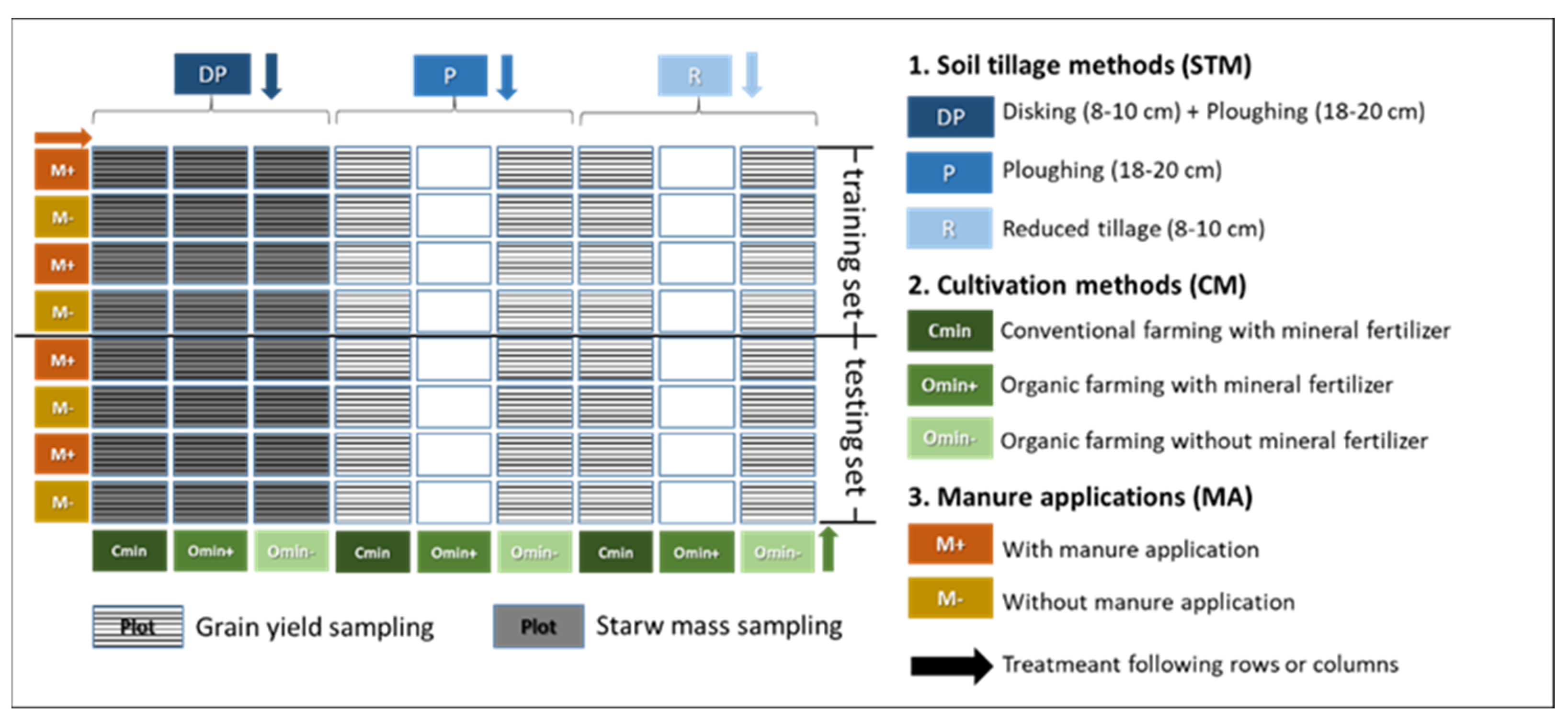
The experimental strategy was established to aid in the recognition of physiological parameters and comparison of yield abilities of the selected varieties and their combinations under three forms of agriculture management practices (AMP): (1) soil tillage methods (STM); (2) cultivation methods (CM); and (3) manure applications (MA), as well as to demonstrate appropriate farming methods to local farmers. Figure 2 shows the AMPs and their specific arrangement in SW, P + O, and SB + RC fields. Every field comprised 72 plots, with a total of 216 plots. Based on considerations of budget limitations, labor shortages, excessive scope, and repetitiveness, the sampling of grain yield was taken from 56 out of 72 plots (n = 56), and straw biomass was sampled from 24 out of 72 plots (n = 24) specific from the disking and ploughing (DP) area (Figure 2). The harvesting took place on 5 August 2019 in field SB + RC and on 16 August 2019 in fields SW and P + O. The fresh grain and biomass were weighed by plot and dried to verify the dry grain yield and fresh straw mass measured in kilograms per hectare. However, regarding the mixture P + O field, the total weight of the two crops was calculated, while in the SB + RC field only the SB grain yield and straw mass.

2.2. Hyperspectral Image Data Collection

Airborne measurements were carried out in Kuusiku Agricultural Research Centre on 18 June 2019 using hyperspectral imager HySpex (Norsk Elektro Optikk AS (NEO), Oslo, Norway) owned by Estonian Marine Institute and operated by the Estonian Land Board. HySpex was flown at an altitude of 900 m which resulted in a spatial resolution of 40 cm (Figure 1a). The spectral resolution of HySpex is approximately 2.69 nm (216 spectral bands ranging from visible to near-infrared with centers between 409 nm and 989 nm). The day was sunny with a wind speed of 2.6 m/s, average air temperature of 10 °C. Regarding the growth stages of the main crops on the flight date, spring wheat, spring barley, and oat were approximately in the booting to heading stage. The mixed crops, i.e., field pea and red clover were in the reproductive growth stages and the flowing stage, respectively.
Raw HySpex image data were converted into units of spectral radiance (W m−2 nm−1 sr−1) using Rad software developed by the NEO. PARGE (Parametric Geocoding, ReSe Applications Schäpfler, University of Zurich) geo-coding software was used for geo correction of the flight lines utilizing accurate altitude and location measurements provided by the GPS/INS unit. The captured Hyspex flight line used in this study is shown in Figure 2. Atmospheric influence at such a low altitude was considered minimal and therefore atmospheric correction was not applied to the imagery.

2.3. Hyperspectral Image Processing

Most hyperspectral processing techniques now employ commercial software such as Erdas Imagine, ENVI, or the MATLAB hyperspectral toolbox [70]. These technologies are often expensive and can have limited statistical analysis capabilities. Therefore, we employed a new package that was built on the open-source software R in 2019. The hyperspectral data analysis (Hsdar) package incorporates several important hyperspectral capabilities from the HyperSpec package [71], with an emphasis on the analysis of large data sets collected in the field for vegetation remote sensing. It is available at https://CRAN.R-project.org/package=hsdar (accessed on 20 July 2021) on the Comprehensive R Archive Network (CRAN).
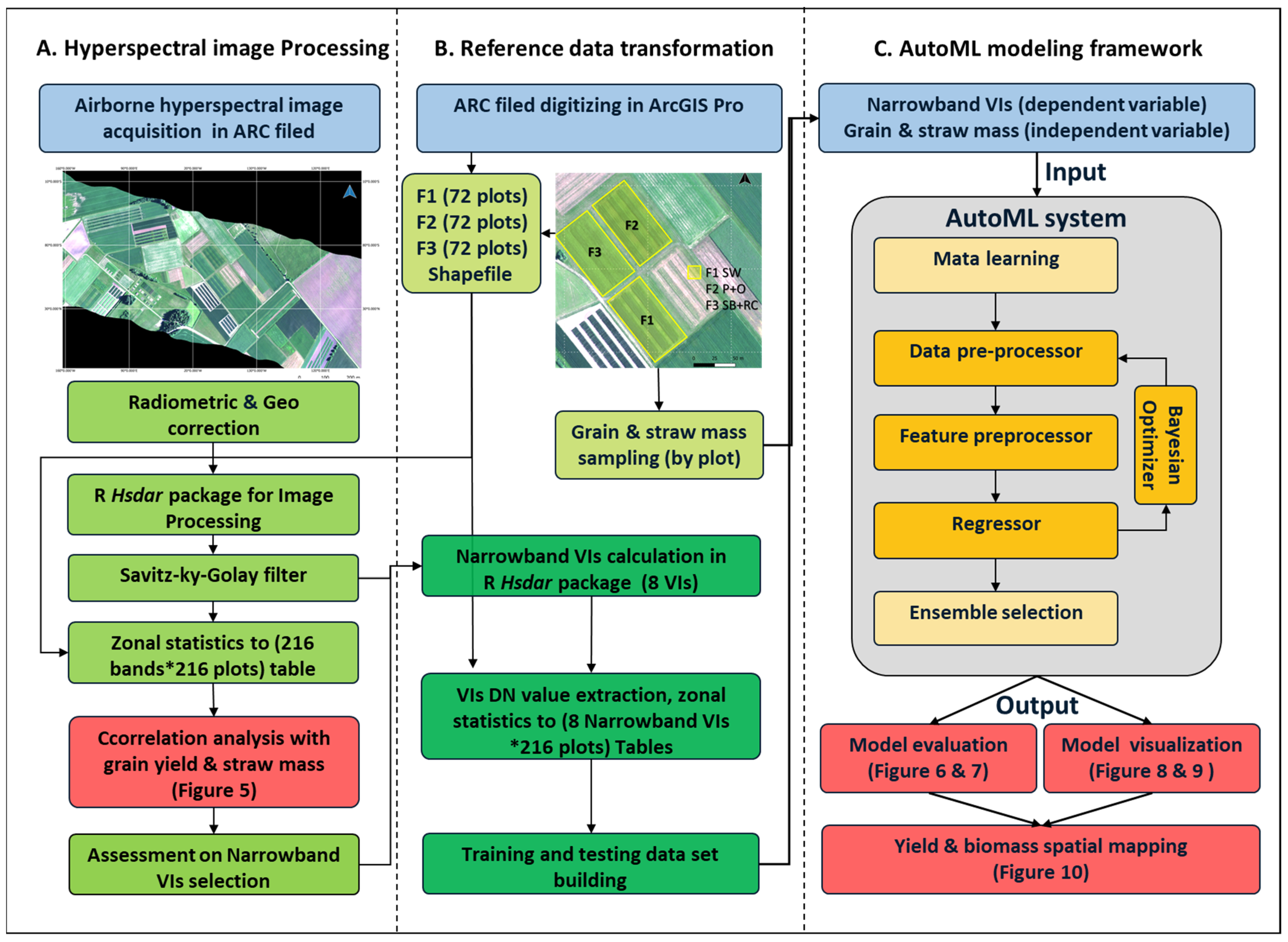
In our study, hyperspectral data were reconstructed into a class named ‘Speclib’ to offer a framework for handling huge sets in R. This allows the user to store three-dimensional (3D) cube data together with extra adding information into a matrix. This matrix, together with the wavelength information can then be utilized in the Hsdar software and used to manage subsequent calculations. A Savitz-ky-Golay filter (method “sgolay”) with a length of 15 nm was used in the initial preprocessing stage to reduce noise from the spectra. By fitting a polynomial function to the reflectance data, the filter minimizes noise and removes minor discrepancies between adjacent bands. These noise-reduced hyperspectral data were calculated zonal statistics and converted to a (216 (wavelength bands) multiplied by 216 (plot Shapefile)) table. This table was then subsequently used for preliminary correlation analysis between grain yield and straw mass with the mean wavelength reflectance value into plot level (Figure 3A). The correlation analysis results of each narrowband band can be utilized as a consideration in the following selection of narrowband vegetation indexes.

2.4. Narrowband Vegetation Index

Optical indices for chlorophyll estimation studies have focused on analyzing reflectance in specific narrow bands, ratios, combinations, and the properties of derivative spectra to minimize extraneous factor changes and increase sensitivity to chlorophyll content [6]. In this study, we targeted VIs that were sensitive to canopy structure, biochemistry, and physiology, and those that might potentially indicate variance in grain yields and biomass in our study. Pigments (i.e., chlorophyll a, chlorophyll b, and carotenoids) exhibit varied spectral behavior from an optical standpoint, with specific absorption properties at different wavelengths [72]. Therefore, we employed pre-defined indices in the Hsdar R package to automatically fit provided wave-length positions and compute corresponding VIs to reduce the intricacy of computation and boost the repeatability of this research (Table 1).
During our study, the Normalized Difference Vegetation Index (NDVI) was adopted based on it is sensitivity to green leaf area or green leaf biomass, and it can be used to monitor photosynthetically active vegetation biomass distribution using linear combinations of red and infrared radiances [73]. However, it is crucial to note that NDVI has a saturation effect at richer vegetation covers [74]. To solve the probable saturation problem, NDVI2 was applied with its ability to adequately determine chlorophyll in the presence of a high-pigment concentration background [75]. The renormalized difference vegetation index (RDVI) narrow band was employed in this study due to its capacity in identifying mixture phytomass in grassland [76]. The prospect for using the Transformed Chlorophyll Absorption in Reflectance Index (TCARI) in an operational remote sensing situation in the context of precision agriculture was investigated. The R700/R670 ratio was chosen to reduce the combined impacts of underlying soil reflectance and non-photosynthetic materials. The changes in reflectance characteristics of background materials (soil and non-photosynthetic components) and the R700/R550 ratio are strongly connected to differences in background materials [6,77]. Soil-Adjusted Vegetation Index (SAVI) was conducted to reduce soil-induced fluctuations in vegetations using a transformation approach to decrease soil brightness impacts by counting red and near-infrared wavelengths from spectral data [78]. Optimized Soil-Adjusted Vegetation Index (OSAVI) with two types of reflectance combinations (OSAVI and OSAVI2) was selected for its simplicity of use in the context of deployable observations on agricultural landscapes, as its estimation requires no knowledge of soil optical properties, and it also provided the best results for most crops [79], as well as the distinction of tillage effects in an economically RGB UAV application [80]. In addition, the choice of Simple Ratio (SR) narrow-band indices (R515/R550), different from chlorophyll pigment content detection, was based on its feasibility to predict carotene content on hyperspectral imagery in heterogeneous canopies [81]. Carotenoid concentrations reveal important information about plant physiological state [82], and offering a heterogeneous VI source may improve model predictability and minimize collinearity.
These narrowband VIs were computed and saved in TIFF file format (https://www.adobe.io/open/standards/TIFF.html accessed on 15 July 2021), which were then utilized to extract spatial information in the SW, P + O, and SB + RC experimental fields. For extraction, a total of 216 plots were digitized in ArcGIS Pro [85]. Average VIs across every plot were extracted and determined at each plot at the research location, while one-meter buffer zones were calculated inwards from each plot boundary to eliminate unexpected boundary effects. Considering the potential variances in the treatment of each AMP, we divided the field from the center of the area into training and testing areas equally, ensuring that the training area contained all combinations of AMPs (Figure 2). These collected parameters were then utilized in this study to create AutoML algorithms for estimating and evaluating grain production and straw mass.

2.5. AutoML Regression with Auto-Sklearn

This study employed the robust and frequently updated AutoML system, Auto-sklearn, based on the scikit-learn ML library in Python [86]. It employs 15 classifiers, 14 feature processing, and four data pre-processing methods, yielding a 110-hyperparameter structured hypothesis space [62,87]. It offers an advancement on existing AutoML approaches by incorporating prior performance on comparable datasets and generates ensembles from the models that were examined throughout the optimization procedure (Figure 3C). This technique involves the largely configurable ML prototype with the automatically generated ML pipelines, i.e., feature selection (deleting trivial features), transformation (reducing dimensionality), and hyperparameter optimization based on Bayesian optimization strategy sequential model-based algorithm configuration (SMAC) [88]. Following that, a Random Forest [89] approach was utilized for fast cross-validation, assessing one-fold at a time and eliminating poor-performing hyperparameter configurations during the initial phases. The Random Forest approach delivers a superior accuracy rate, as well as alternative pipeline operators that boost regression performance within the datasets [62,90].
All computations in this study were performed on an Intel Core i5-1035G1 CPU (1.00 GHz) with 16 GB RAM utilizing the LINUX open-source operating system. The processes outlined in [62] were executed for the AutoML framework. To begin with, the system employs a supplemental technique based on widely used meta-learning procedures to train machine learning models over the statistical features of datasets and evaluates the model parameters that produce the greatest performance [91]. Second, the system creates ensembles of the models that Bayesian optimization examined, using high-performing regressors and pre-processors employed within the ML framework. Finally, the program works a wide range of empirical examinations on a diverse set of data to determine whether the AutoML regression offers better outcomes than previous regressions. However, any strongly correlated VIs should be eliminated during the feature selection step to avoid the effects of collinearity. Since Auto-sklearn works with low-dimensional optimization issues [92], this step was bypassed in this stage. Table 2 lists the principal AutoML regression parameters employed in this study. To perform tests, as a demonstration of the practicability and efficiency of AutoML model selection, CPU timing for each task was restricted to 30 s, and the runtime for assessing a single model to 10 s. The analyses were performed separately for each of the crop fields, with grain yield consisting of 56 plots (n = 56) and straw mass divided in the training and test sites (0.5/0.5) for regression modelling (Figures 6 and 7).

2.6. Model Evaluation

The assessment was carried out for the prediction of AutoML models (Figures 6 and 7). Performance evaluation approaches proposed by [19,93] were utilized to evaluate each model. The coefficient of determination (R2) (Equation (1) and normalized root means square error (NRMSE) (Equation (2)) were used to evaluate the models’ accuracy. The following are the equations that were used:
R 2 = 1 ( y ^ i y i ) 2 ( y i y ¯ ) 2
N R M S E = ( ( y ^ i y i ) 2 ) / n Δ y  
where: y i is the training dataset’s ith observation value represents the observation value; y ¯ denotes the training dataset’s mean value; y ^ i denotes the model predictions, n denotes the number of observations; and Δ y represents the difference between the training dataset’s lowest and highest values.

3. Results

3.1. The Field Observation DM Data Analysis

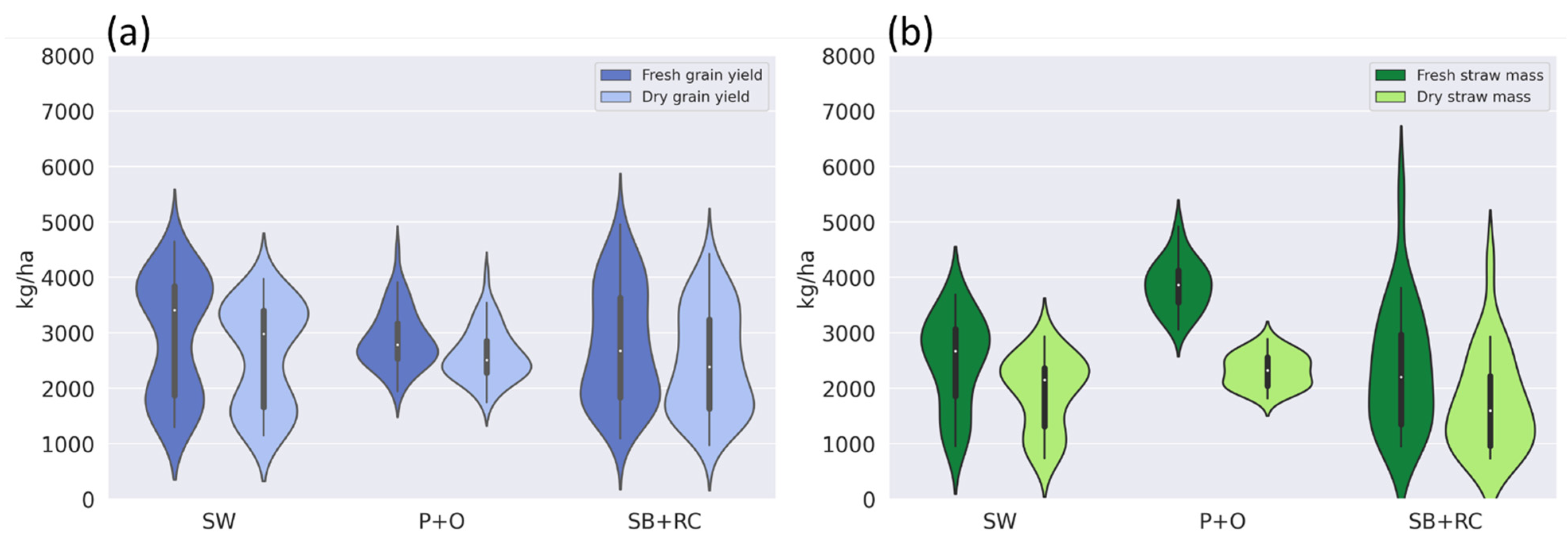
The average actual grain yield and above ground straw mass data (fresh and dry) gathered from the SW, P + O, and SB + RC experimental regions are displayed in the violin plot (Figure 4), where we exhibited the range of grain yield and straw mass data and assembled them by fields since the treatments were interspersed within each plot. In addition, we opted to examine at dry and fresh weight separately since the accumulated rainfall of 4.1 mm (in SW and P + O fields) and 0.4 mm (in SB + RC fields) in the three days before the two harvests (on 16 August 2019, and 5 August 2019, respectively) may have contributed to increased fresh weight with additional water content.

3.2. The Hyperspectral Reflectance Signature under Various Agriculture Management Practises

Figure 4 displays a mean reflectance plot produced from hyperspectral data of SW, P + O, and SB + RC fields, with enclosed subsets categorized by (Figure 5A) soil tillage method (STM) and (Figure 5B) cultivation method (CM) agricultural operations. Regarding agricultural management practices, the wavelength bands between 700–750 nm and 760–900 nm had significant identification capabilities, while the 400–700 nm region showed little differentiation between management practices. The cultivation method (Figure 4B) provides greater recognition ability (separation) in this range when compared with STM spectral information (Figure 5A). In terms of crop types, spring wheat monocropping seemed to give a better ability to recognize AMPs, followed by mixed cropping systems SB + RC and P + O fields. However, since the focus of this study was on grain yield and biomass prediction, we omitted the narrowband VIs wave range based on the strong absorption bands near 760 nm and excluded them from subsequent AutoML analyses.

3.3. Characterization of the Correlation Coefficient with Averaged Radiance Hyperspectral Data and Field Observation

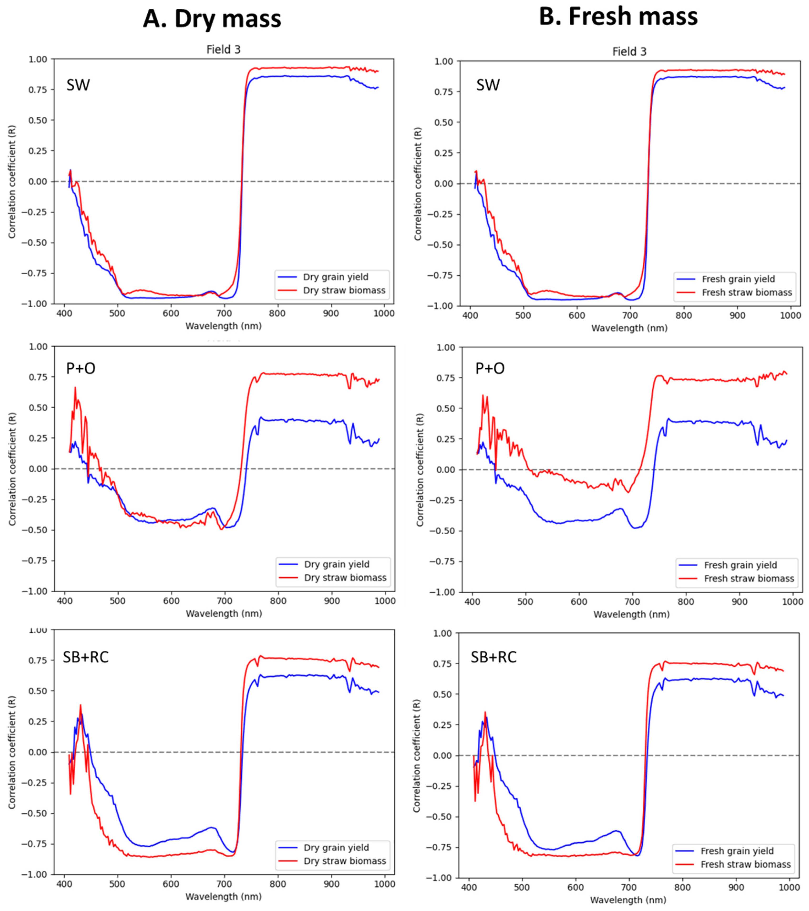
Correlation Coefficient (r) was used as exploratory analysis in our study and as a reference for subsequent modelling. Figure 5 shows the correlation coefficients (r) between each averaged hyperspectral narrow-band data with the dry mass (Figure 6A) and fresh mass (Figure 6B) at the plot level. The pattern of positive r values was typically obtained with reflectance between 750–940 nm wavelengths, whereas the strong negative correlation with reflectance was between 500–700 nm. Moreover, we also observed that the correlation of straw mass (red line) was stronger than grain yield (blue line) at all fields in the 750–1000 nm range. By comparison, the results showed that, in the patterning of r curves, SW was closely associated with highly positive and negative r values in dry mass (Figure 6A), while with the lower correlation nearby the oxygen absorption peak was 760 nm. This tendency was observed in our previous reflectance signature analysis as well. Among the three fields, P + O had the least correlation. Regarding the fresh mass (Figure 5B), the correlation and spectral characteristics were comparable to the weight of the dry mass. Except for 740–750 nm, SW had overall the strongest correlation, followed by SB + RC and P + O.

3.4. The AutoML Model Prediction and Evaluation

In this study, the narrowband VIs reflectance of grain yield (n = 56) and straw mass (n = 24) based on training/testing (0.5/0.5) principles were used for AutoML modelling, respectively. The AutoML framework was used to test the appropriate combinations of data set parameters throughout the modelling process. Scatter plots representing model predictions and observed weight values (kg ha−1) were compared to the coefficient of the determination (R2) and normalized root means square error (NRMSE) along with the 1:1 line.
Figure 7 shows the regression plots of fresh (Figure 7A) grain yield (kg ha−1) and (Figure 7B) straw mass (kg ha−1) in SW, P + O, and SB + RC fields based on narrowband VIs and AutoML methods. The results indicated that, in fresh grain yield (Figure 7A), the AutoML model had the lowest prediction errors (NRMSE = 0.13) and the highest R2 value (0.95) in SW field, followed by SB + RC field (NRMSE = 0.16, R2 = 0.88) and P + O (NRMSE = 0.16, R2 = 0.88). Even though the three models functioned well, there was a minor non-uniform bias found within the models, with an underestimation of grain yields in areas with higher output in SW and SB + RC fields. On the other hand, for fresh straw mass, the SW field remains the best performing among the other fields with (NRMSE = 0.16, R2 = 0.88) followed by the SB + RC field (NRMSE = 0.27, R2 = 0.77) with uniform overestimation bias, and P + O (NRMSE = 0.25, R2 = 0.56) (Figure 7B). Among them, P + O’s prediction ability was insufficient, and the reference data collected were concentrated in the 3000 to 5000 (kg ha−1) interval, which makes the regression model unable to be effectively extended.
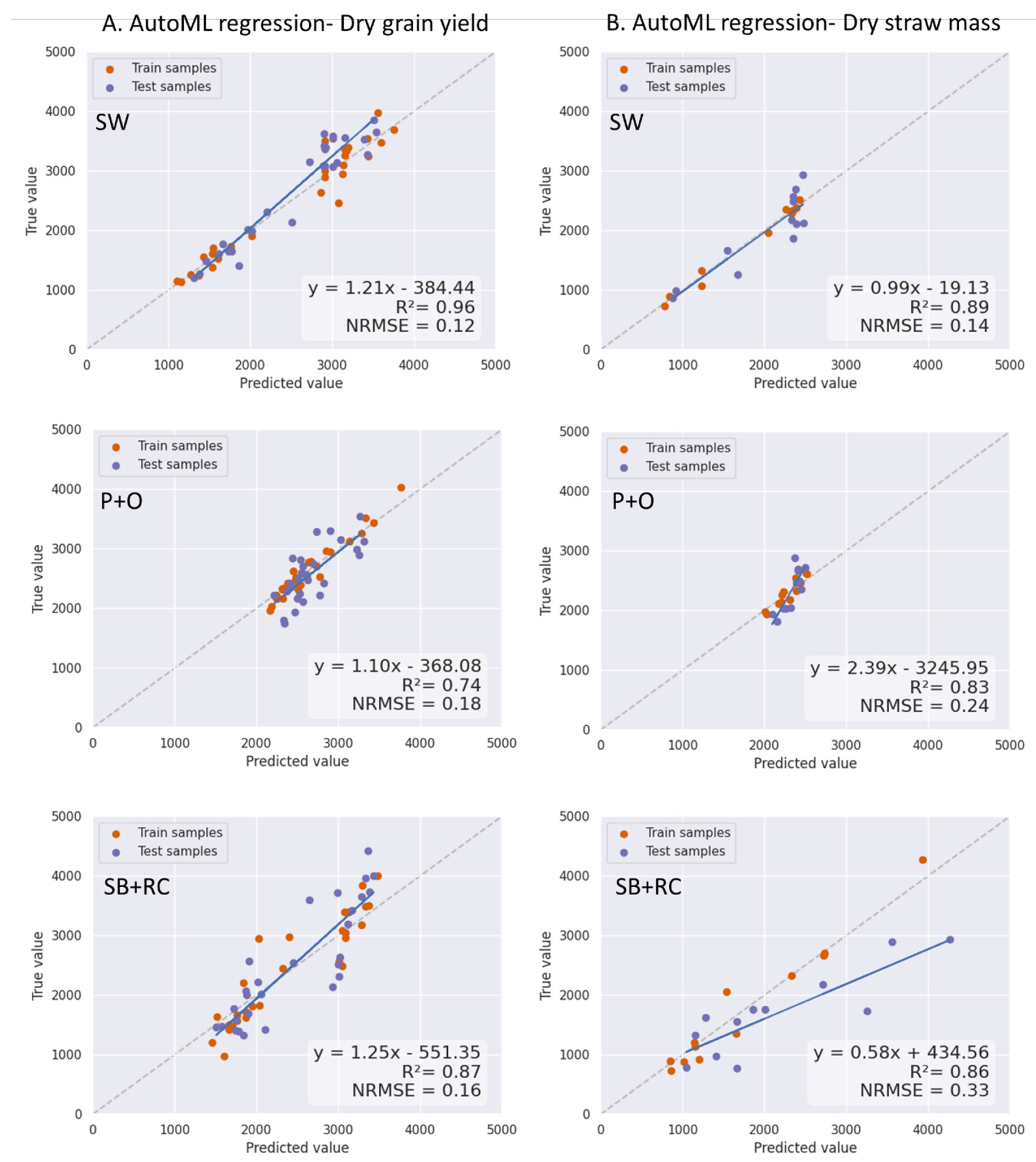
Figure 8 demonstrates the behavior of predictive models utilizing dry (A) grain yield (kg ha−1) and (B) straw mass (kg ha−1) in SW, P + O, and SB + RC fields based on narrowband VIs and AutoML methods. The results specified that, in summary, SW yielded the best performance for dry grain yield (NRMSE = 0.12, R2 = 0.96) and straw mass (NRMSE = 0.15, R2 = 0.89) among SB + RC, and P + O files (Figure 8A). Compared with the fresh mass model, the dry performance was better in general, especially in the dry straw model of SB + RC (NRMSE = 0.33, R2 = 0.86) and P + O (NRMSE = 0.24, R2 = 0.83) (Figure 8B), although these two models had a larger degree of bias under the comparison of 1:1 slope.

3.5. The AutoML Model Pipeline Visualization

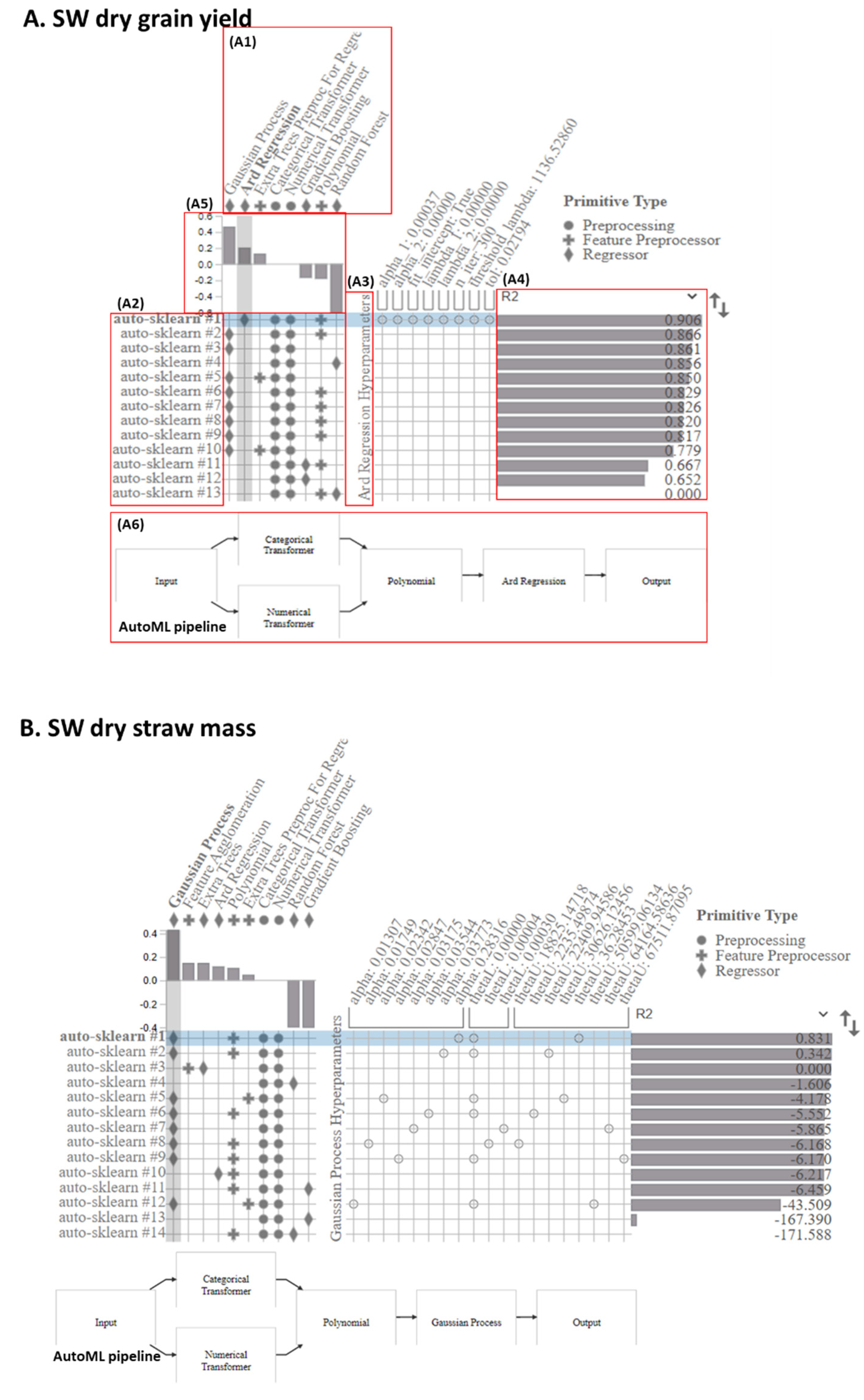
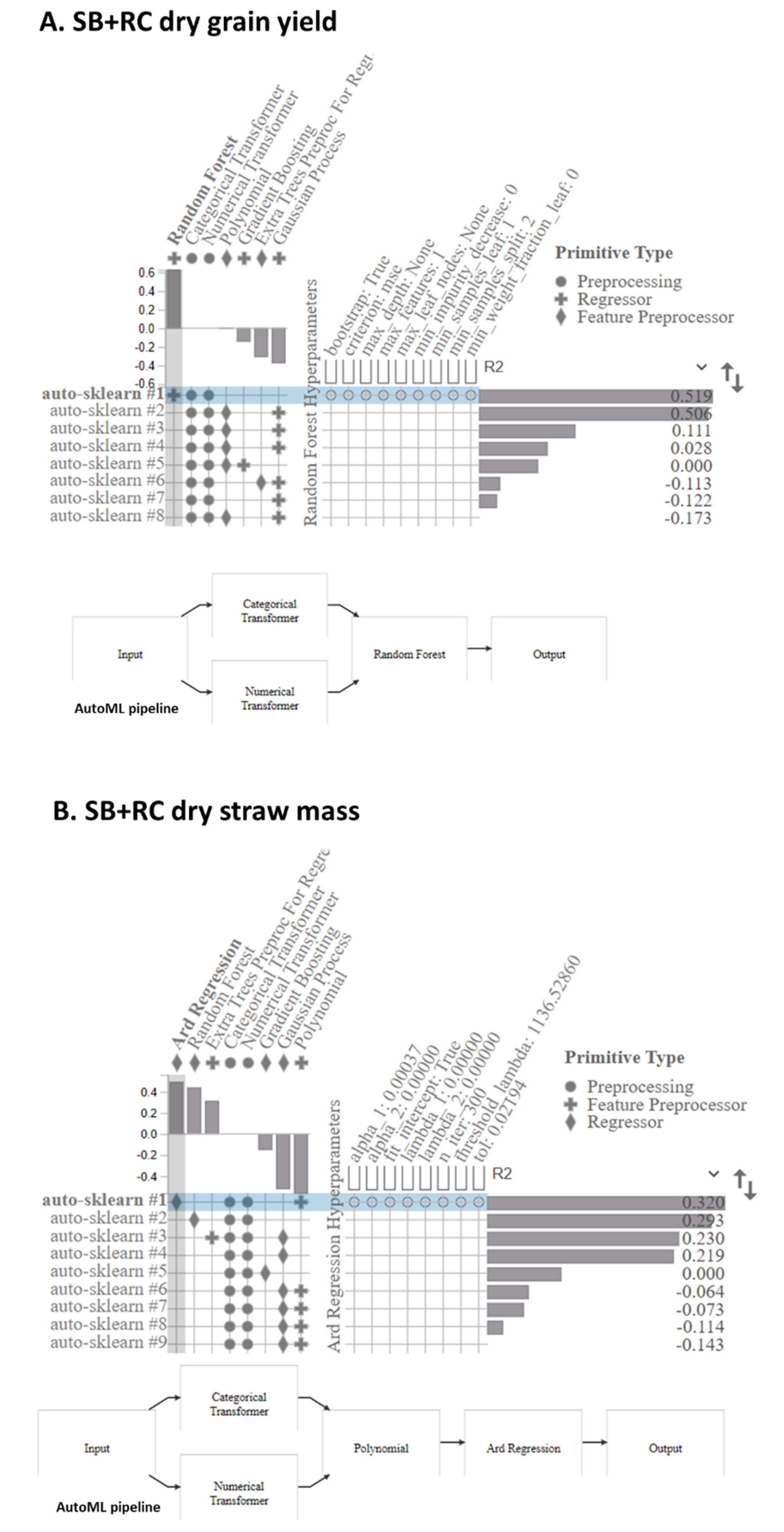
An interactive AutoML visualization tool PipelineProfiler [94] was used in this study (Figure 9). To simplify the description, we only list the best regression modelling results across two crop fields (SW and SB + RC) with the evaluation performance of AutoML pipeline execution times set at 30 s, the primitive comparison against other regressors in the same pipeline, and real-time hyperparameter selections. The results confirmed that the best regressor found for dry grain yield was automatic relevance determination (Ard) Regression [95] for the SW field (Figure 9A), and for the SB + RC field, it was the Random Forest [89] (Figure 10A), while for dry straw mass, it was Gaussian Process [96] (Figure 9B) for the SW field, and Ard Regression for the SB + RC field (Figure 10B), with all hyperparameters found by AutoML also displayed in the figures.

3.6. The Field Observation DM Data Analysis

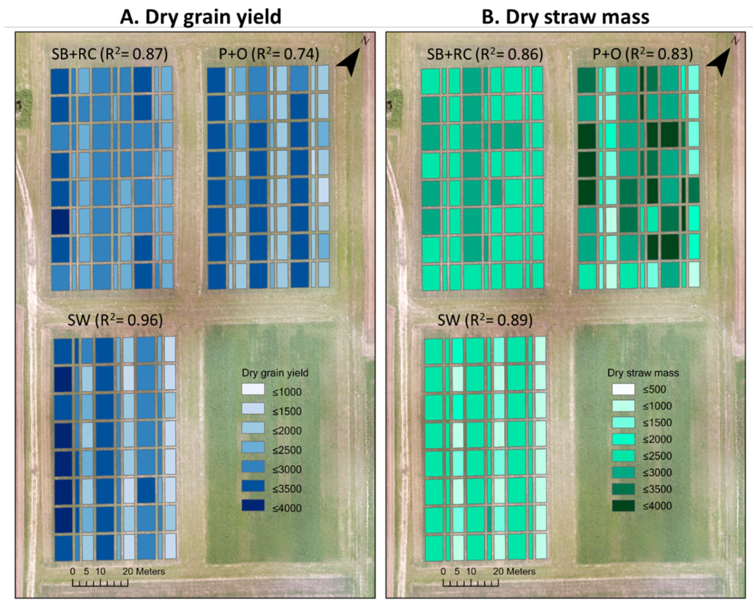
Based on the AutoML models provided above (Figure 7 and Figure 8), a series of prediction maps were generated (Figure 11) for dry grain yield and straw mass for SW, P + O, and SB + RC experimental sites at the plot level. Furthermore, the SW and P + O fields’ prediction capabilities were 60 days before the harvest date (18 June–16 August), whereas the SB + RC field’s estimating was 49 days before harvest (18 June–5 August).

4. Discussion

This research demonstrated an automatic, open-sourced, rapid, and non-destructive framework by using hyperspectral narrow-band vegetation indexes under regular mono- and mixed cultivation for crop grain yield and straw mass modelling. Since the investigation was carried out under a diversity of agricultural management practices, the methods and findings can profoundly aid agronomists and farmers in designing accurate cropping systems to enhance environmental assessment.

4.1. The Effect of Hyperspectral Signatures and the Correlation between Crop Yield and Straw Mass

The initial goal of this study was to conduct an exploratory evaluation of the hyperspectral reflectance signature and determine the ideal narrowband VIs for modelling common crop types and farming schedules in Northern Europe. To identify redundant bands and establish wavebands that could best help AutoML regression modelling, the VIs were first chosen based on prior knowledge of the literature and then filtered by the reflectance signature (Figure 5) and their Correlation Coefficients with yield and biomass (Figure 6). Although there was no general focus on a formal classification analysis in our current study, the characteristics of hyperspectral data under different agricultural practices (i.e., STM, CM, and MA) are still worthy of attention.
Figure 5 reveals that, in general, because chlorophyll absorption is not limited to the center wavelength but also affects adjacent bands, we can see that reflectance values in the blue and red sections are significantly reduced, resulting in “absorption characteristics” in the spectral signature of the reflectance in all spectral results. In addition, all the reflection spectra showed obvious absorption peaks at 760 nm. This spectral region is influenced by atmospheric oxygen [97,98] and, therefore, this region was avoided while calculating VI’s. Additionally, from the results, the wavelength range 750–900 nm (NIR) had strong recognition capabilities based on the variation of reflection intensity; however, the 400–700 nm (visible bands) region was inefficient and offered little separation or discernment. The differentiation on spectra at the wavelength range of 750–900 nm suggested that the interior leaf structure, biochemical concentration, and water content of the target vegetation are different. A previous study pointed out that the diversity of NIR regions is usually caused by differences in internal leaf structure [99]. However, reflectance variation at the canopy level may be due to additional factors like LAI, canopy design, and backdrop soil [100]. These results will be valuable for further classification activities in agriculture management recognition.
The coefficients correlation (r) of each narrow-band with both grain yield and straw mass exhibited a similar pattern of r curves for both dry (Figure 6A) and fresh weight (Figure 6B) analysis, yet r in absolute values for the P + O field was observed to be less correlated than those for grain yield and straw mass, especially in the fresh weight. This is because the P + O field was mixed cultivation and the source of weight is the sum of the two crops and the amount of precipitation before harvesting may indirectly bring about a lower degree of correlation. Interestingly, while the findings of these linear correlation tests all showed that the straw mass has a stronger link with the spectrum, it does not depend on the empirical model’s degree of fit (see Figure 7 and Figure 8). Hence, we discovered that grain yield (R2) had a superior goodness-of-fit performance than straw mass in general, with lower NRMSE.

4.2. The Hyperspectral Narrowband VIs and AutoML Modelling

Despite the opportunities afforded by hyperspectral systems to collect a multitude of spectrum data, extracting the relevant important wavelengths from a data cube can be challenging [101]. In our study, we used hyperspectral narrowband VIs as predictors for AutoML modelling. However, we avoided selecting narrowband VIs with spectrums that might be affected by atmospheric oxygen. With this in mind, the target VIs selected for analysis were extracted, calculated, and processed in the modelling stage, which reduced processing and storage demands.
Based on the empirical AutoML regression model, the estimation capacity of hyperspectral narrowband VIs was exceptional. The best coefficient of determination for mono-cultivated wheat was 0.96, for mixed peas and oats was 0.76, and for mixed legumes and spring barley was 0.88. In terms of straw mass estimation, they were 0.98, 0.83, and 0.86 respectively. We determined that the prediction ability of dry weight was typically greater than that of fresh weight, especially in fields where mixed peas and oats, which was 27 per cent higher. This demonstrated that the crop water content has an influence on the model’s estimation outputs to a certain extent.
According to a previous study, spectral measurements were taken during the Tillering II and Heading phases in wheat yielded the best results for estimating biophysical factors using narrowband VIs [42]. This is consistent with our recommended flight time. In addition, different band combinations can be effectively utilized since crop circumstances change according to factors such as management conditions and soil characteristics. Others have demonstrated that piecewise multiple regression models on narrow bands provide for greater flexibility in selecting the bands that provide the most information at a given stage of crop development [102]. This viewpoint has also been confirmed in our research.

4.3. The AutoML Method’s Applicability and Impact in Hyperspectral Imaging

In this study, we employed an AutoML framework to assist in self-regulating, instinctive regression operations, as well as enhancing challenging hyperparameter adjustments. This method advances the use of hyperspectral imaging in farm-scaled environmental and crop phenotypic activity and possesses several advantages.
Firstly, the flexibility of implementation. With the ever-increasing variability of remote sensing systems and the requirement for empirical model choices, the constraints of adjusting unidentified background parameters are being addressed. This means that many existing models that have been under-optimized in the past now have the chance to be re-modelled using artificial intelligence-based machines to relearn the performance tasks.
Secondly, the alleviation of learning costs. Experience tells us that computer learning for remote-sensed images frequently necessitates a large number of samples and a lengthy learning period, i.e., deep learning [103,104,105]. This is incompatible with conventional agricultural experimental sampling procedures, which are limited by personnel, the complexity of the experiment design, and the number of repetitions. While, AutoML practices the Random Forest (RF) method [89] for fast cross-validation, testing one-fold at a time and weeding out underperformance hyperparameter choices, for example, the combined algorithm selection and hyperparameter optimization (CASH) problems [62]. It boasts novel pipeline operators that increase the goodness of fit of datasets significantly. The RF approach is well-known for assessing lower sample sizes and increasing the performance of small datasets. [89,106]. In addition, the AutoML framework quickly provided promising regressors and hyperparameter selections. In our research, each run of the regression model only took thirty seconds of learning time. This considerably improves learning efficiency, the ability to find an appropriate formula in the time allotted, and reduces the requirement for machine learning expertise [87,107].
Thirdly, the capacity of innovation. It is noticeable that random forest (RF), support vector machine (SVM), and artificial neural network (ANN) algorithms are among the most widely employed ML techniques in a wide range of recent remote sensing-based studies [108]. Their practicality and performance have been confirmed by many, but equally, there are still other similarly applicable ML methods that may have been shelved. As shown in Figure 9 and Figure 10, the Ard regressors [109,110] and Gaussian Processors [96] were chosen as the best regressors for the grain yield and biomass tasks. These algorithms have received less attention and reference in remote sensing studies. These results indicated that AutoML can uncover alternative ML methods that would otherwise be overlooked by investigators when working with regression subjects.

4.4. The Limitations in This Study

The location, soil types, chosen crop categories, and varieties present may be restricted in this study. In addition, it is important to note that we did not address yield comparisons under different agricultural management approaches since the intricacy of the experimental design may have led to inadequate sampling numbers, as well as possible interaction effects. However, we have presented a framework that can be applied to numerous test regions and the necessity to moderately reduce the number of samples by using AutoML. In addition, due to the limits of the current Auto-Sklearn system, not all regressors performed could be backtracked in our research to explore the individual feature importance ranking, which limits their capacity to aid in the selection of suitable VIs. However, our attempts to provide a wide range of continuous and selectable narrow-band spectral information (over 216 spectral bands) resulted in improved performance.

5. Conclusions

Our study highlights the capability of hyperspectral analysis for yield and biomass prediction in complex design fields through the use of two significant open-sourced software systems: the R language hyperspectral processing package and Python’s Auto-Sklearn machine learning technology. The performance evaluation with several types of hyperspectral vegetation indicators we employed to characterize crop production and straw mass was satisfactory. We suggest they can be further applied to other crop biophysical characteristics. The VIs we suggest, as well as automatic narrowband VI calculation, might minimize data redundancy and cleaning time, as well as the computational power hardware requirements. It is also envisaged that further agricultural cultivation practices could be classified using hyperspectral imaging in the NIR spectral region (750–900 nm) with considerable discernible changes in reflectance spectra.
However, the aerial hyperspectral platform utilized in this study may be less cost-effective than fixed-wing or rotary-wing drone systems, which may be more viable for farm-scale exploration. Comprehensive and contemporaneous phenotypic information of products under various agri-environment schemes, as well as their field-based biochemical conditions, reminds us of further challenges which likely exist for remote sensing technology to overcome. Nevertheless, hyperspectral imaging combined with complementary modelling precision, the abundance of spectrum selection flexibility, and extensive flight coverage still have an important role at this stage.
In conclusion, our research focused on the integration and implementation of the hyperspectral imaging and AutoML framework approach with various crop types under multifunctional agriculture management fields in response to crop biomass/yield estimation. Under common crops and cultivation in most Nordic countries, it will provide agricultural decision-makers with professional yield estimation and sustainable agricultural management advice. The study also revealed that the anticipated yield may be advanced two months before harvest. That is, spring wheat, spring barley, and oat were approximately in the booting to heading stage, field pea was around the reproductive growth stages, and the red clover field was in the flowering stage (49 days before in our case). The emergence of the AutoML system has helped to increase the application and effectiveness of remote sensing-based data analysis technology. However, more research and experiments will be required in the future to advance and validate the automatic learning framework’s true potential and usage.

Author Contributions

Conceptualization, K.-Y.L.; methodology, K.-Y.L. and R.S.d.L.; software, K.-Y.L., R.S.d.L., E.V. and V.H.C.P.; validation, N.G.B.; formal analysis, K.-Y.L. and V.H.C.P.; investigation, R.S.d.L., E.V. and K.S. (Karli Sepp); resources, T.K. and K.S. (Kalev Sepp); data curation, K.-Y.L., R.S.d.L., E.V., T.K. and K.S. (Karli Sepp); writing—original draft preparation, K.-Y.L.; writing—review and editing, N.G.B., T.K., K.S. (Karli Sepp), V.H.C.P., M.-D.Y., A.V. and K.S. (Kalev Sepp); supervision, N.G.B., T.K. and K.S. (Kalev Sepp); funding acquisition, K.S. (Kalev Sepp). All authors have read and agreed to the published version of the manuscript.

Funding

This research was funded by the European Regional Development Fund within the Estonian National Programme for Addressing Socio-Economic Challenges through R&D (RITA): L180283PKKK, Estonian Research Council grant PUT PRG302, Estonian IT Academy financed by European Social Fund, and the Doctoral School of Earth Sciences and Ecology, financed by the European Union, European Regional Development Fund (Estonian University of Life Sciences ASTRA project “Value-chain based bio-economy”).

Data Availability Statement

The data presented in this study are available on request from the corresponding author. The data are not publicly available due to the data size.

Acknowledgments

We give respect and gratitude to the scikit-learn framework’s developers and maintainers, as well as the Auto-sklearn interface developed at the University of Freiberg. This work was also supported by the Kuusiku Variety Testing Centre of Agricultural Research Centre in Estonia, and the Estonian IT Academy (English brand name StudyITin.ee) which has been financed by the European Social Fund.

Conflicts of Interest

The authors declare no conflict of interest.

Appendix A

Figure A1. Daily climograph of the study area (Kuusiku) during the crop growing period from April to August in 2019. The blue bars and the red line represent the daily average of rainfall and temperature, respectively.
Remotesensing 14 01114 g0a1

References

  1. Pavón-Pulido, N.; López-Riquelme, J.A.; Torres, R.; Morais, R.; Pastor, J.A. New Trends in Precision Agriculture: A Novel Cloud-Based System for Enabling Data Storage and Agricultural Task Planning and Automation. Precis. Agric. 2017, 18, 1038–1068. [Google Scholar] [CrossRef]
  2. Karthikeyan, L.; Chawla, I.; Mishra, A.K. A Review of Remote Sensing Applications in Agriculture for Food Security: Crop Growth and Yield, Irrigation, and Crop Losses. J. Hydrol. 2020, 586, 124905. [Google Scholar] [CrossRef]
  3. Wen, W.; Timmermans, J.; Chen, Q.; van Bodegom, P.M. A Review of Remote Sensing Challenges for Food Security with Respect to Salinity and Drought Threats. Remote Sens. 2021, 13, 6. [Google Scholar] [CrossRef]
  4. Yang, M.D.; Huang, K.S.; Kuo, Y.H.; Tsai, H.P.; Lin, L.M. Spatial and Spectral Hybrid Image Classification for Rice Lodging Assessment through UAV Imagery. Remote Sens. 2017, 9, 583. [Google Scholar] [CrossRef] [Green Version]
  5. Mandal, A.; Majumder, A.; Dhaliwal, S.S.; Toor, A.S.; Mani, P.K.; Naresh, R.K.; Gupta, R.K.; Mitran, T. Impact of Agricultural Management Practices on Soil Carbon Sequestration and Its Monitoring through Simulation Models and Remote Sensing Techniques: A Review. Crit. Rev. Environ. Sci. Technol. 2020, 52, 1–49. [Google Scholar] [CrossRef]
  6. Haboudane, D.; Miller, J.R.; Tremblay, N.; Zarco-Tejada, P.J.; Dextraze, L. Integrated Narrow-Band Vegetation Indices for Prediction of Crop Chlorophyll Content for Application to Precision Agriculture. Remote Sens. Environ. 2002, 81, 416–426. [Google Scholar] [CrossRef]
  7. Sahoo, R.N.; Ray, S.S.; Manjunath, K.R. Hyperspectral Remote Sensing of Agriculture. Curr. Sci. 2015, 108, 848–859. [Google Scholar] [CrossRef]
  8. Windfuhr, M.; Jonsén, J. Food Sovereignty towards Democracy in Localized Food Systems; FAO: Rome, Italy, 2005; Volume 339. [Google Scholar]
  9. Gómez, D.; Salvador, P.; Sanz, J.; Casanova, J.L. Potato Yield Prediction Using Machine Learning Techniques and Sentinel 2 Data. Remote Sens. 2019, 11, 1745. [Google Scholar] [CrossRef] [Green Version]
  10. Triplett, G.B.; Dick, W.A. No-Tillage Crop Production: A Revolution in Agriculture! Agron. J. 2008, 100, 153–165. [Google Scholar] [CrossRef]
  11. Karlen, D.L.; Kovar, J.L.; Cambardella, C.A.; Colvin, T.S. Thirty-Year Tillage Effects on Crop Yield and Soil Fertility Indicators. Soil Tillage Res. 2013, 130, 24–41. [Google Scholar] [CrossRef] [Green Version]
  12. Ashapure, A.; Jung, J.; Yeom, J.; Chang, A.; Maeda, M.; Maeda, A.; Landivar, J. A Novel Framework to Detect Conventional Tillage and No-Tillage Cropping System Effect on Cotton Growth and Development Using Multi-Temporal UAS Data. ISPRS J. Photogramm. Remote Sens. 2019, 152, 49–64. [Google Scholar] [CrossRef]
  13. Telles, T.S.; Reydon, B.P.; Maia, A.G. Effects of No-Tillage on Agricultural Land Values in Brazil. Land Use Policy 2018, 76, 124–129. [Google Scholar] [CrossRef]
  14. Fanigliulo, R.; Antonucci, F.; Figorilli, S.; Pochi, D.; Pallottino, F.; Fornaciari, L.; Grilli, R.; Costa, C. Light Drone-Based Application to Assess Soil Tillage Quality Parameters. Sensors 2020, 20, 728. [Google Scholar] [CrossRef] [PubMed] [Green Version]
  15. Desta, B.T.; Gezahegn, A.M.; Tesema, S.E. Impacts of Tillage Practice on the Productivity of Durum Wheat in Ethiopia. Cogent Food Agric. 2021, 7, 1869382. [Google Scholar] [CrossRef]
  16. Crews, T.E.; Peoples, M.B. Legume versus Fertilizer Sources of Nitrogen: Ecological Tradeoffs and Human Needs. Agric. Ecosyst. Environ. 2004, 102, 279–297. [Google Scholar] [CrossRef]
  17. Zikeli, S.; Gruber, S.; Teufel, C.F.; Hartung, K.; Claupein, W. Effects of Reduced Tillage on Crop Yield, Plant Available Nutrients and Soil Organic Matter in a 12-Year Long-Term Trial under Organic Management. Sustainability 2013, 5, 3876–3894. [Google Scholar] [CrossRef] [Green Version]
  18. Yang, X.M.; Drury, C.F.; Reynolds, W.D.; Reeb, M.D. Legume Cover Crops Provide Nitrogen to Corn during a Three-Year Transition to Organic Cropping. Agron. J. 2019, 111, 3253–3264. [Google Scholar] [CrossRef] [Green Version]
  19. Li, K.Y.; Burnside, N.G.; de Lima, R.S.; Peciña, M.V.; Sepp, K.; der Yang, M.; Raet, J.; Vain, A.; Selge, A.; Sepp, K. The Application of an Unmanned Aerial System and Machine Learning Techniques for Red Clover-Grass Mixture Yield Esti-Mation under Variety Performance Trials. Remote Sens. 2021, 13, 1994. [Google Scholar] [CrossRef]
  20. Loide, V. The Results of an NPK-Fertilisation Trial of Long-Term Crop Rotation on Carbonate-Rich Soil in Estonia. Acta Agric. Scand. Sect. B Soil Plant Sci. 2019, 69, 596–605. [Google Scholar] [CrossRef]
  21. Gianelle, D.; Vescovo, L.; Marcolla, B.; Manca, G.; Cescatti, A. Ecosystem Carbon Fluxes and Canopy Spectral Reflectance of a Mountain Meadow. Int. J. Remote Sens. 2009, 30, 435–449. [Google Scholar] [CrossRef]
  22. Seitz, S.; Goebes, P.; Puerta, V.L.; Pereira, E.I.P.; Wittwer, R.; Six, J.; van der Heijden, M.G.A.; Scholten, T. Conservation Tillage and Organic Farming Reduce Soil Erosion. Agron. Sustain. Dev. 2019, 39, 4. [Google Scholar] [CrossRef] [Green Version]
  23. Doyle, C.J.; Topp, C.F.E. The Economic Opportunities for Increasing the Use of Forage Legumes in North European Livestock Systems under Both Conventional and Organic Management. Renew. Agric. Food Syst. 2004, 19, 15–22. [Google Scholar] [CrossRef]
  24. Laidig, F.; Piepho, H.P.; Drobek, T.; Meyer, U. Genetic and Non-Genetic Long-Term Trends of 12 Different Crops in German Official Variety Performance Trials and on-Farm Yield Trends. Theor. Appl. Genet. 2014, 127, 2599–2617. [Google Scholar] [CrossRef] [PubMed] [Green Version]
  25. Lollato, R.P.; Roozeboom, K.; Lingenfelser, J.F.; da Silva, C.L.; Sassenrath, G. Soft Winter Wheat Outyields Hard Winter Wheat in a Subhumid Environment: Weather Drivers, Yield Plasticity, and Rates of Yield Gain. Crop Sci. 2020, 60, 1617–1633. [Google Scholar] [CrossRef]
  26. Andrade, J.F.; Rattalino Edreira, J.I.; Mourtzinis, S.; Conley, S.P.; Ciampitti, I.A.; Dunphy, J.E.; Gaska, J.M.; Glewen, K.; Holshouser, D.L.; Kandel, H.J.; et al. Assessing the Influence of Row Spacing on Soybean Yield Using Experimental and Producer Survey Data. Field Crops Res. 2019, 230, 98–106. [Google Scholar] [CrossRef]
  27. Munaro, L.B.; Hefley, T.J.; DeWolf, E.; Haley, S.; Fritz, A.K.; Zhang, G.; Haag, L.A.; Schlegel, A.J.; Edwards, J.T.; Marburger, D.; et al. Exploring Long-Term Variety Performance Trials to Improve Environment-Specific Genotype × Management Recommendations: A Case-Study for Winter Wheat. Field Crops Res. 2020, 255, 107848. [Google Scholar] [CrossRef]
  28. Frazier, A.E. Landscape Heterogeneity and Scale Considerations for Super-Resolution Mapping. Int. J. Remote Sens. 2015, 36, 2395–2408. [Google Scholar] [CrossRef]
  29. Ge, Y.; Chen, Y.; Stein, A.; Li, S.; Hu, J. Enhanced Subpixel Mapping with Spatial Distribution Patterns of Geographical Objects. IEEE Trans. Geosci. Remote Sens. 2016, 54, 2356–2370. [Google Scholar] [CrossRef]
  30. Feng, W.; Yao, X.; Zhu, Y.; Tian, Y.C.; Cao, W.X. Monitoring Leaf Nitrogen Status with Hyperspectral Reflectance in Wheat. Eur. J. Agron. 2008, 28, 394–404. [Google Scholar] [CrossRef]
  31. Thorp, K.R.; Wang, G.; Bronson, K.F.; Badaruddin, M.; Mon, J. Hyperspectral Data Mining to Identify Relevant Canopy Spectral Features for Estimating Durum Wheat Growth, Nitrogen Status, and Grain Yield. Comput. Electron. Agric. 2017, 136, 1–12. [Google Scholar] [CrossRef] [Green Version]
  32. Tsouros, D.C.; Bibi, S.; Sarigiannidis, P.G. A Review on UAV-Based Applications for Precision Agriculture. Information 2019, 10, 349. [Google Scholar] [CrossRef] [Green Version]
  33. Raeva, P.L.; Šedina, J.; Dlesk, A. Monitoring of Crop Fields Using Multispectral and Thermal Imagery from UAV. Eur. J. Remote Sens. 2019, 52, 192–201. [Google Scholar] [CrossRef] [Green Version]
  34. Baret, F.; Guyot, G.; Major, D.J. TSAVI: A Vegetation Index Which Minimizes Soil Brightness Effects on LAI and APAR Estimation. In Proceedings of the Digest—International Geoscience and Remote Sensing Symposium (IGARSS), Vancouver, BC, Canada, 10–14 July 1989; Volume 3. [Google Scholar]
  35. Qi, J.; Chehbouni, A.; Huete, A.R.; Kerr, Y.H.; Sorooshian, S. A Modified Soil Adjusted Vegetation Index. Remote Sens. Environ. 1994, 48, 119–126. [Google Scholar] [CrossRef]
  36. Rhyma, P.P.; Norizah, K.; Hamdan, O.; Faridah-Hanum, I.; Zulfa, A.W. Integration of Normalised Different Vegetation Index and Soil-Adjusted Vegetation Index for Mangrove Vegetation Delineation. Remote Sens. Appl. Soc. Environ. 2020, 17, 100280. [Google Scholar] [CrossRef]
  37. Zhou, G. Determination of Green Aboveground Biomass in Desert Steppe Using Litter-Soil-Adjusted Vegetation Index. Eur. J. Remote Sens. 2014, 47, 611–625. [Google Scholar] [CrossRef]
  38. Mutanga, O.; Skidmore, A.K. Narrow Band Vegetation Indices Overcome the Saturation Problem in Biomass Estimation. Int. J. Remote Sens. 2004, 25, 3999–4014. [Google Scholar] [CrossRef]
  39. Zarco-Tejada, P.J.; Ustin, S.L.; Whiting, M.L. Temporal and Spatial Relationships between Within-Field Yield Variability in Cotton and High-Spatial Hyperspectral Remote Sensing Imagery. Agron. J. 2005, 97, 641–653. [Google Scholar] [CrossRef] [Green Version]
  40. Haboudane, D.; Miller, J.R.; Pattey, E.; Zarco-Tejada, P.J.; Strachan, I.B. Hyperspectral Vegetation Indices and Novel Algorithms for Predicting Green LAI of Crop Canopies: Modeling and Validation in the Context of Precision Agriculture. Remote Sens. Environ. 2004, 90, 337–352. [Google Scholar] [CrossRef]
  41. Monteiro, P.F.C.; Filho, R.A.; Xavier, A.C.; Monteiro, R.O.C. Assessing Biophysical Variable Parameters of Bean Crop with Hyperspectral Measurements. Sci. Agric. 2012, 69, 87–94. [Google Scholar] [CrossRef] [Green Version]
  42. Xavier, A.C.; Theodor Rudorff, B.F.; Moreira, M.A.; Alvarenga, B.S.; de Freitas, J.G.; Salomon, M.V. Hyperspectral Field Reflectance Measurements to Estimate Wheat Grain Yield and Plant Height. Sci. Agric. 2006, 63, 130–138. [Google Scholar] [CrossRef] [Green Version]
  43. Stagakis, S.; Markos, N.; Sykioti, O.; Kyparissis, A. Monitoring Canopy Biophysical and Biochemical Parameters in Ecosystem Scale Using Satellite Hyperspectral Imagery: An Application on a Phlomis Fruticosa Mediterranean Ecosystem Using Multiangular CHRIS/PROBA Observations. Remote Sens. Environ. 2010, 114, 977–994. [Google Scholar] [CrossRef]
  44. Zarco-Tejada, P.J.; Miller, J.R.; Noland, T.L.; Mohammed, G.H.; Sampson, P.H. Scaling-up and Model Inversion Methods with Narrowband Optical Indices for Chlorophyll Content Estimation in Closed Forest Canopies with Hyperspectral Data. IEEE Trans. Geosci. Remote Sens. 2001, 39, 1491–1507. [Google Scholar] [CrossRef] [Green Version]
  45. Zarco-Tejada, P.J. Hyperspectral Remote Sensing of Closed Forest Canopies: Estimation of Chlorophyll Fluorescence and Pigment Content; York University: Toronto, ON, Canada, 2000. [Google Scholar]
  46. Schmidt, K.S.; Skidmore, A.K. Spectral Discrimination of Vegetation Types in a Coastal Wetland. Remote Sens. Environ. 2003, 85, 92–108. [Google Scholar] [CrossRef]
  47. Feng, J.; Jiao, L.; Liu, F.; Sun, T.; Zhang, X. Unsupervised Feature Selection Based on Maximum Information and Minimum Redundancy for Hyperspectral Images. Pattern Recognit. 2016, 51, 295–309. [Google Scholar] [CrossRef]
  48. Yang, M.D.; Huang, K.H.; Tsai, H.P. Integrating MNF and HHT Transformations into Artificial Neural Networks for Hyperspectral Image Classification. Remote Sens. 2020, 12, 2327. [Google Scholar] [CrossRef]
  49. Bajcsy, P.; Groves, P. Methodology for Hyperspectral Band Selection. Photogramm. Eng. Remote Sens. 2004, 70, 793–802. [Google Scholar] [CrossRef]
  50. Heiskanen, J.; Rautiainen, M.; Stenberg, P.; Mõttus, M.; Vesanto, V.H. Sensitivity of Narrowband Vegetation Indices to Boreal Forest LAI, Reflectance Seasonality and Species Composition. ISPRS J. Photogramm. Remote Sens. 2013, 78, 1–14. [Google Scholar] [CrossRef]
  51. Näsi, R.; Viljanen, N.; Kaivosoja, J.; Alhonoja, K.; Hakala, T.; Markelin, L.; Honkavaara, E. Estimating Biomass and Nitrogen Amount of Barley and Grass Using UAV and Aircraft Based Spectral and Photogrammetric 3D Features. Remote Sens. 2018, 10, 1082. [Google Scholar] [CrossRef] [Green Version]
  52. Li, C.; Ma, C.; Pei, H.; Feng, H.; Shi, J.; Wang, Y.; Chen, W.; Li, Y.; Feng, X.; Shi, Y. Estimation of Potato Biomass and Yield Based on Machine Learning from Hyperspectral Remote Sensing Data. J. Agric. Sci. Technol. B 2020, 10, 195–213. [Google Scholar] [CrossRef]
  53. Choudhury, M.R.; Das, S.; Christopher, J.; Apan, A.; Chapman, S.; Menzies, N.W.; Dang, Y.P. Improving Biomass and Grain Yield Prediction of Wheat Genotypes on Sodic Soil Using Integrated High-Resolution Multispectral, Hyperspectral, 3d Point Cloud, and Machine Learning Techniques. Remote Sens. 2021, 13, 3482. [Google Scholar] [CrossRef]
  54. Nawar, S.; Corstanje, R.; Halcro, G.; Mulla, D.; Mouazen, A.M. Delineation of Soil Management Zones for Variable-Rate Fertilization: A Review. Adv. Agron. 2017, 143, 175–245. [Google Scholar]
  55. Chlingaryan, A.; Sukkarieh, S.; Whelan, B. Machine Learning Approaches for Crop Yield Prediction and Nitrogen Status Estimation in Precision Agriculture: A Review. Comput. Electron. Agric. 2018, 151, 61–69. [Google Scholar]
  56. Zhang, W.; Zhang, Z.; Chao, H.C.; Guizani, M. Toward Intelligent Network Optimization in Wireless Networking: An Auto-Learning Framework. IEEE Wirel. Commun. 2019, 26, 76–82. [Google Scholar] [CrossRef] [Green Version]
  57. Colombo, R.; Bellingeri, D.; Fasolini, D.; Marino, C.M. Retrieval of Leaf Area Index in Different Vegetation Types Using High Resolution Satellite Data. Remote Sens. Environ. 2003, 86, 120–131. [Google Scholar] [CrossRef]
  58. He, X.; Zhao, K.; Chu, X. AutoML: A Survey of the State-of-the-Art. Knowl.-Based Syst. 2021, 212, 106622. [Google Scholar] [CrossRef]
  59. Mendoza, H.; Klein, A.; Feurer, M.; Springenberg, J.T.; Hutter, F. Towards Automatically-Tuned Neural Networks. In Proceedings of the Workshop on Automatic Machine Learning, New York, NY, USA, 24 June 2016. [Google Scholar]
  60. Yao, Q.; Wang, M.; Chen, Y.; Dai, W.; Hu, Y.Q.; Li, Y.F.; Tu, W.W.; Yang, Q.; Yu, Y. Taking the Human out of Learning Applications: A Survey on Automated Machine Learning. arXiv 2018, arXiv:1810.13306. [Google Scholar]
  61. Thornton, C.; Hutter, F.; Hoos, H.H.; Leyton-Brown, K. Auto-WEKA: Combined Selection and Hyperparameter Optimization of Classification Algorithms. In Proceedings of the ACM SIGKDD International Conference on Knowledge Discovery and Data Mining, Chicago, IL, USA, 11–14 August 2013; pp. 847–855. [Google Scholar] [CrossRef]
  62. Feurer, M.; Klein, A.; Eggensperger, K.; Springenberg, J.T.; Blum, M.; Hutter, F. Efficient and Robust Automated Machine Learning. In Proceedings of the Advances in Neural Information Processing Systems, Montreal, QC, Canada, 7–12 December 2015; Volume 2015. [Google Scholar]
  63. Remeseiro, B.; Bolon-Canedo, V. A Review of Feature Selection Methods in Medical Applications. Comput. Biol. Med. 2019, 112, 103375. [Google Scholar] [CrossRef]
  64. Babaeian, E.; Paheding, S.; Siddique, N.; Devabhaktuni, V.K.; Tuller, M. Estimation of Root Zone Soil Moisture from Ground and Remotely Sensed Soil Information with Multisensor Data Fusion and Automated Machine Learning. Remote Sens. Environ. 2021, 260, 112434. [Google Scholar] [CrossRef]
  65. Koh, J.C.O.; Spangenberg, G.; Kant, S. Automated Machine Learning for High-throughput Image-based Plant Phenotyping. Remote Sens. 2021, 13, 858. [Google Scholar] [CrossRef]
  66. Komer, B.; Bergstra, J.; Eliasmith, C. Hyperopt-Sklearn: Automatic Hyperparameter Configuration for Scikit-Learn. In Proceedings of the 13th Python in Science Conference, Austin, TX, USA, 6–12 July 2014. [Google Scholar]
  67. Lehnert, L.W.; Meyer, H.; Obermeier, W.A.; Silva, B.; Regeling, B.; Thies, B.; Bendix, J. Hyperspectral Data Analysis in R: The Hsdar Package. J. Stat. Softw. 2019, 89, 1–23. [Google Scholar] [CrossRef] [Green Version]
  68. R Core Team. R: A Language and Environment for Statistical Computing; R Foundation for Statistical Computing: Vienna, Austria, 2020. [Google Scholar]
  69. FAO. World Reference Base for Soil Resources; World Soil Resources Report 103; FAO: Rome, Italy, 2006; ISBN 9251055114. [Google Scholar]
  70. The Mathworks Inc. MATLAB (R2019a), Version 9.6.0.1072779; The MathWorks Inc.: Natick, MA, USA, 2019.
  71. Beleites, C. Unstable Laser Emission Vignette for the Data Set Laser of the R Package HyperSpec. Spectrosc. Laser 2021, 75, 1–6. [Google Scholar]
  72. Blackburn, G.A. Spectral Indices for Estimating Photosynthetic Pigment Concentrations: A Test Using Senescent Tree Leaves. Int. J. Remote Sens. 1998, 19, 657–675. [Google Scholar] [CrossRef]
  73. Tucker, C.J. Red and Photographic Infrared Linear Combinations for Monitoring Vegetation. Remote Sens. Environ. 1979, 8, 127–150. [Google Scholar] [CrossRef] [Green Version]
  74. Fernández-Manso, A.; Fernández-Manso, O.; Quintano, C. SENTINEL-2A Red-Edge Spectral Indices Suitability for Discriminating Burn Severity. Int. J. Appl. Earth Obs. Geoinf. 2016, 50, 170–175. [Google Scholar] [CrossRef]
  75. Gitelson, A.; Merzlyak, M.N. Quantitative Estimation of Chlorophyll-a Using Reflectance Spectra: Experiments with Autumn Chestnut and Maple Leaves. J. Photochem. Photobiol. B Biol. 1994, 22, 247–252. [Google Scholar] [CrossRef]
  76. Vescovo, L.; Wohlfahrt, G.; Balzarolo, M.; Pilloni, S.; Sottocornola, M.; Rodeghiero, M.; Gianelle, D. New Spectral Vegetation Indices Based on the Near-Infrared Shoulder Wavelengths for Remote Detection of Grassland Phytomass. Int. J. Remote Sens. 2012, 33, 2178–2195. [Google Scholar] [CrossRef] [Green Version]
  77. Kim, M.S.; Daughtry, C.S.T.; Chappelle, E.W.; McMurtrey, J.E.; Walthall, C.L. The Use of High Spectral Resolution Bands for Estimating Absorbed Photosynthetically Active Radiation (A Par). In Proceedings of the 6th Symposium on Physical Measurements and Signatures in Remote Sensing, Val d’Isère, France, 17–21 January 1994. [Google Scholar]
  78. Huete, A.R. A Soil-Adjusted Vegetation Index (SAVI). Remote Sens. Environ. 1988, 25, 295–309. [Google Scholar] [CrossRef]
  79. Rondeaux, G.; Steven, M.; Baret, F. Optimization of Soil-Adjusted Vegetation Indices. Remote Sens. Environ. 1996, 55, 95–107. [Google Scholar] [CrossRef]
  80. Yeom, J.; Jung, J.; Chang, A.; Ashapure, A.; Maeda, M.; Maeda, A.; Landivar, J. Comparison of Vegetation Indices Derived from UAV Data for Differentiation of Tillage Effects in Agriculture. Remote Sens. 2019, 11, 1548. [Google Scholar] [CrossRef] [Green Version]
  81. Hernández-Clemente, R.; Navarro-Cerrillo, R.M.; Zarco-Tejada, P.J. Carotenoid Content Estimation in a Heterogeneous Conifer Forest Using Narrow-Band Indices and PROSPECT + DART Simulations. Remote Sens. Environ. 2012, 127, 32–46. [Google Scholar] [CrossRef]
  82. Demmig-Adams, B.; Adams, W.W. Photoprotection and Other Responses of Plants to High Light Stress. Annu. Rev. Plant Physiol. Plant Mol. Biol. 1992, 43, 599–626. [Google Scholar] [CrossRef]
  83. Wu, C.; Niu, Z.; Tang, Q.; Huang, W. Estimating Chlorophyll Content from Hyperspectral Vegetation Indices: Modeling and Validation. Agric. For. Meteorol. 2008, 148, 1230–1241. [Google Scholar] [CrossRef]
  84. Roujean, J.L.; Breon, F.M. Estimating PAR Absorbed by Vegetation from Bidirectional Reflectance Measurements. Remote Sens. Environ. 1995, 51, 375–384. [Google Scholar] [CrossRef]
  85. ESRI. ArcGIS PRO: Essential Workflows; ESRI: Redlands, CA, USA, 2016. [Google Scholar]
  86. Pedregosa, F.; Varoquaux, G.; Gramfort, A.; Michel, V.; Thirion, B.; Grisel, O.; Blondel, M.; Prettenhofer, P.; Weiss, R.; Dubourg, V.; et al. Scikit-Learn: Machine Learning in Python. J. Mach. Learn. Res. 2011, 12, 2825–2830. [Google Scholar]
  87. Feurer, M.; Eggensperger, K.; Falkner, S.; Lindauer, M.; Hutter, F. Auto-Sklearn 2.0: The Next Generation. arXiv 2020, arXiv:2007.0407424. [Google Scholar]
  88. Hutter, F.; Hoos, H.H.; Leyton-Brown, K. Sequential Model-Based Optimization for General Algorithm Configuration. In Proceedings of the Lecture Notes in Computer Science (Including Subseries Lecture Notes in Artificial Intelligence and Lecture Notes in Bioinformatics); Springer: Berlin/Heidelberg, Germany, 2011; Volume 6683. [Google Scholar]
  89. Breiman, L. Random Forests. Mach. Learn. 2001, 24, 123–140. [Google Scholar] [CrossRef] [Green Version]
  90. Olson, R.S.; Urbanowicz, R.J.; Andrews, P.C.; Lavender, N.A.; Kidd, L.C.; Moore, J.H. Automating Biomedical Data Science through Tree-Based Pipeline Optimization. In Proceedings of the Lecture Notes in Computer Science (Including Subseries Lecture Notes in Artificial Intelligence and Lecture Notes in Bioinformatics); Springer: Berlin/Heidelberg, Germany, 2016; Volume 9597. [Google Scholar]
  91. Franceschi, L.; Frasconi, P.; Salzo, S.; Grazzi, R.; Pontil, M. Bilevel Programming for Hyperparameter Optimization and Meta-Learning. In International Conference on Machine Learning; PMLR; 2018; Volume 80, pp. 1568–1577. Available online: http://proceedings.mlr.press/v80/franceschi18a.html?ref=https://githubhelp.com (accessed on 26 January 2022).
  92. Feurer, M.; Springenberg, J.T.; Hutter, F. Initializing Bayesian Hyperparameter Optimization via Meta-Learning. In Proceedings of the National Conference on Artificial Intelligence, Austin, TX, USA, 25–30 January 2015; Volume 2. [Google Scholar]
  93. Yue, J.; Yang, G.; Li, C.; Li, Z.; Wang, Y.; Feng, H.; Xu, B. Estimation of Winter Wheat Above-Ground Biomass Using Unmanned Aerial Vehicle-Based Snapshot Hyperspectral Sensor and Crop Height Improved Models. Remote Sens. 2017, 9, 708. [Google Scholar] [CrossRef] [Green Version]
  94. Ono, J.P.; Castelo, S.; Lopez, R.; Bertini, E.; Freire, J.; Silva, C. PipelineProfiler: A Visual Analytics Tool for the Exploration of AutoML Pipelines. IEEE Trans. Vis. Comput. Graph. 2021, 27, 390–400. [Google Scholar] [CrossRef]
  95. Qi, Y.; Minka, T.P.; Picard, R.W.; Ghahramani, Z. Predictive Automatic Relevance Determination by Expectation Propagation. In Proceedings of the Twenty-First International Conference on Machine Learning, ICML 2004, Banff, AB, Canada, 4–8 July 2004. [Google Scholar]
  96. Seeger, M. Gaussian Processes for Machine Learning. Int. J. Neural Syst. 2004, 14, 69–106. [Google Scholar] [CrossRef] [Green Version]
  97. Van Diedenhoven, B.; Hasekamp, O.P.; Aben, I. Surface Pressure Retrieval from SCIAMACHY Measurements in the O2A Band: Validation of the Measurements and Sensitivity on Aerosols. Atmos. Chem. Phys. Discuss. 2005, 5, 2109–2120. [Google Scholar] [CrossRef] [Green Version]
  98. Riris, H.; Rodriguez, M.; Mao, J.; Allan, G.; Abshire, J. Airborne Demonstration of Atmospheric Oxygen Optical Depth Measurements with an Integrated Path Differential Absorption Lidar. Opt. Express 2017, 25, 29307–29327. [Google Scholar] [CrossRef]
  99. Gitelson, A.A.; Gritz, Y.; Merzlyak, M.N. Relationships between Leaf Chlorophyll Content and Spectral Reflectance and Algorithms for Non-Destructive Chlorophyll Assessment in Higher Plant Leaves. J. Plant Physiol. 2003, 160, 271–282. [Google Scholar] [CrossRef] [PubMed]
  100. Darvishzadeh, R.; Skidmore, A.; Atzberger, C.; van Wieren, S. Estimation of Vegetation LAI from Hyperspectral Reflectance Data: Effects of Soil Type and Plant Architecture. Int. J. Appl. Earth Obs. Geoinf. 2008, 10, 358–373. [Google Scholar] [CrossRef]
  101. Martínez-Usó, A.; Pla, F.; Sotoca, J.M.; García-Sevilla, P. Clustering-Based Hyperspectral Band Selection Using Information Measures. Proc. IEEE Trans. Geosci. Remote Sens. 2007, 45, 4158–4171. [Google Scholar]
  102. Thenkabail, P.S.; Smith, R.B.; de Pauw, E. Hyperspectral Vegetation Indices and Their Relationships with Agricultural Crop Characteristics. Remote Sens. Environ. 2000, 71, 158–182. [Google Scholar] [CrossRef]
  103. Lecun, Y.; Bengio, Y.; Hinton, G. Deep Learning. Nature 2015, 521, 436–444. [Google Scholar] [CrossRef]
  104. Yang, M.D.; Tseng, H.H.; Hsu, Y.C.; Tsai, H.P. Semantic Segmentation Using Deep Learning with Vegetation Indices for Rice Lodging Identification in Multi-Date UAV Visible Images. Remote Sens. 2020, 12, 633. [Google Scholar] [CrossRef] [Green Version]
  105. Yang, M.D.; Boubin, J.G.; Tsai, H.P.; Tseng, H.H.; Hsu, Y.C.; Stewart, C.C. Adaptive Autonomous UAV Scouting for Rice Lodging Assessment Using Edge Computing with Deep Learning EDANet. Comput. Electron. Agric. 2020, 179, 683–696. [Google Scholar] [CrossRef]
  106. Luan, J.; Zhang, C.; Xu, B.; Xue, Y.; Ren, Y. The Predictive Performances of Random Forest Models with Limited Sample Size and Different Species Traits. Fish. Res. 2020, 227, 105534. [Google Scholar] [CrossRef]
  107. Feurer, M.; Hutter, F. Towards Further Automation in AutoML. In Proceedings of the ICML 2018 AutoML Workshop, Bangkok, Thailand, 25–28 October 2018. [Google Scholar]
  108. Ma, L.; Li, M.; Ma, X.; Cheng, L.; Du, P.; Liu, Y. A Review of Supervised Object-Based Land-Cover Image Classification. ISPRS J. Photogramm. Remote Sens. 2017, 130, 277–293. [Google Scholar] [CrossRef]
  109. Neal, R. Bayesian Learning for Neural Networks. In Lecture Notes in Statistics; Springer: New York, NY, USA, 1996; Volume 1. [Google Scholar]
  110. Mackay, D.J.C. Probable Networks and Plausible Predictions—A Review of Practical Bayesian Methods for Supervised Neural Networks. Netw. Comput. Neural Syst. 1995, 6, 469. [Google Scholar] [CrossRef]
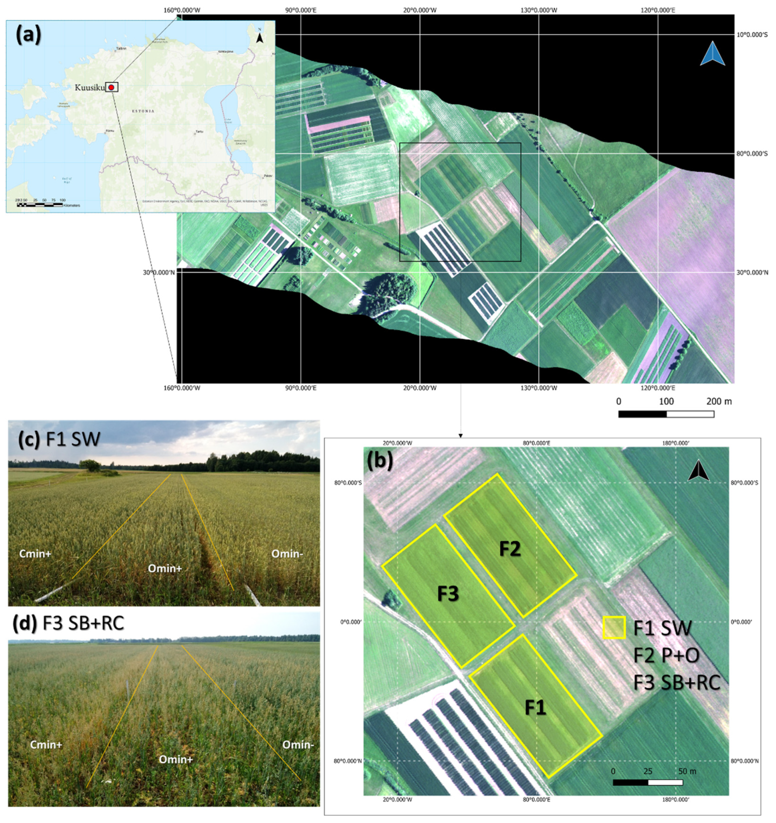
Figure 1. Airborne push-broom hyperspectral image in the Agricultural Research Centre (ARC), Kuusiku, Estonia. (a) Hyperspectral image with the band combination: band 83 (630 nm), band 47 (532 nm), and band 22 (465 nm) light in. (b) The experiment fields of this study, where Field 1 (F1): spring wheat (SW), Field 2 (F2): pea and oat mixture (P + O), and Field 3 (F3): spring barley with under-sowing red clover (SB + RC). The interpretation diagrams represent on-site (c) single variety planting SW, and (d) mixed planting SB + RC.
Remotesensing 14 01114 g001
Figure 2. The structure of agriculture management practices (AMPs) and the sampling method of grain yield and straw mass in the SW, P + O, and SB + RC fields. The AMPs contain three treatments: 1. soil tillage method (STM), 2. cultivation method (CM), and manure application (MA), where the grain yield (n = 56) (black striped rectangle box) and straw mass (n = 24) (grey rectangle box). To guarantee that the training area contained all combinations of AMPs, each field was split into training and testing areas equally from the center. The special arrangements of AMP categories and the sampling method were the same in the three fields.
Remotesensing 14 01114 g002
Figure 3. The flowchart of the hyperspectral image processing and AutoML framework was utilized in this study. (A) The hyperspectral image processing framework where hyperspectral imager HySpex was conducted and R Hsdar package was employed in the processing steps. (B) Field reference data transformation, ARC field were digitized based on each field and following AMP treatments. The grain yield and straw mass data were collected according to plots. Eight narrowband VIs were selected and calculated and segmented into corresponding plot digital numbers (DN) for AutoML modelling. (C) To achieve robust performance, the Auto-sklearn framework automatically built ML pipelines that were provided by the Bayesian optimization method with warm-started meta-learning and combined with a post hoc ensemble building strategy (Adapted with permission from ref. [62] 2019 Springer).
Remotesensing 14 01114 g003
Figure 4. Violin plots of mean harvest results of fresh and dry (a) grain yield and (b) straw mass, grouped by spring wheat (SW), pea and oat mixture (P + O), and spring barley with under-sowing red clover (SB + RC) fields. White dots represent the median, while thick black bars in the center demonstrate interquartile ranges, and black lines represent the remainder of the distribution. The shape of the violins shows point density and data distribution as a whole.
Remotesensing 14 01114 g004
Figure 5. Mean radiance plot derived from hyperspectral data of spring wheat (SW), pea and oat mixture (P + O), and spring barley with under-sowing red clover (SB + RC) fields, grouped by (A) soil tillage method (STM) and (B) cultivation method (CM) farming operations with contained subsets. The wavelength ranges from the visible to near-infrared (VNIR, 400–1000 nm).
Remotesensing 14 01114 g005
Figure 6. The Pearson Correlation Coefficient (r) between the field observation value (grain yield (A); Straw mass (B)) and averaged hyperspectral radiance at the plot level in SW, P + O, and SB + RC region.
Remotesensing 14 01114 g006
Figure 7. Regression plots of (A) fresh grain yield (kg ha−1) and (B) fresh straw mass (kg ha−1) in SW, P + O, and SB + RC fields based on narrowband VIs and AutoML methods. The horizontal axis in the scatter plots represents the model’s projected grain yield or straw mass, while the vertical axis represents field-observed data. Where the R2 = coefficient of determination, NRMSE = normalized root represents the squared error, while the 1:1 slope is shown by the black dotted line.
Remotesensing 14 01114 g007
Figure 8. Regression plots of (A) dry grain yield (kg ha−1) and (B) dry straw mass (kg ha−1) in SW, P + O, and SB + RC fields based on narrowband VIs and AutoML methods. The horizontal axis in the scatter plots represents the model’s projected grain yield or straw mass, while the vertical axis represents field-observed data. Where R2 = coefficient of determination, NRMSE = normalized root means squared error, and the black dotted line exemplifies the 1:1 slope.
Remotesensing 14 01114 g008
Figure 9. The interactive AutoML pipeline matrix plots with thirty-second running-time limits sorted by coefficient of determination (R2) performance (A,B). (A) Spring wheat (SW) dry grain yield pipeline matrix with the Top1 regressor, automatic relevance determination (Ard) regression, where (A1) illustrated Primitives (in columns) used by the pipelines (A2) the blue line (in rows) showed the best R2 rank); (A3) one-hot-encoded hyperparameters (in columns) for the primitive across pipelines, (A4) R2 performance ranking of AutoML pipelines; (A5) Primitive contribution view demonstrating the correlations between pipeline scores and primitive usage are displayed in A5. The Gaussian Process showed the highest correlation score regarding R2 performance; (A6) step-by-step AutoML Pipeline algorithm flowchart, where the box before the output represents the regressor of the model (in A6 Ard regression as the regressor). (B) Spring wheat (SW) dry straw mass field pipeline matrix with the Top1 regressor, Gaussian Process.
Remotesensing 14 01114 g009
Figure 10. The interactive AutoML pipeline matrix plots with thirty-second running-time limits sorted by coefficient of determination (R2) performance (A,B). (A) spring barley with under-sowing red clover (SB + RC) dry grain yield pipeline matrix with the Top1 regressor, Random Forest. The rows display a blue line representing the best R2 rank followed by its hyperparameters settings; (B) SB + RC dry straw mass pipeline matrix with the Top1 regressor, Ard regression, followed by its hyperparameters settings.
Remotesensing 14 01114 g010
Figure 11. The spatial prediction mapping output of (A) dry grain yield (kg ha−1) and (B) dry straw mass (kg ha−1) in SW, P + O, and SB + RC fields based on their respective AutoML prediction models at the plot level. The performing coefficient of determination (R2) is displayed in the previous results.
Remotesensing 14 01114 g011
Table 1. Descriptions and formulae of narrowband VIs were utilized in this study. Narrowband VIs were calculated, which were closest to the wavelengths given in the original Hsdar R package references.
Vegetation IndexDescriptionEquationReference
NDVINormalized Difference Vegetation Index (R800 − R680)/(R800 + R680)[73]
NDVI2Normalized Difference Vegetation Index 2(R750−R705)/(R750 + R705)[75]
OSAVIOptimized Soil Adjusted Vegetation Index(1 + 0.16) × (R800 − R670)/(R800 + R670 + 0.16)[79]
OSAVI2Optimized Soil Adjusted Vegetation Index 2(1 + 0.16) × (R750 − R705)/(R750 + R705 + 0.16)[83]
RDVIRenormalized Difference Vegetation Index(R800 − R670)/√(R800 + R670)[84]
SRSimple Ratio R515/R550[81]
SAVISoil-Adjusted Vegetation Index(1 + L 1) × (R800 − R670)/(R800 + R670 + L)[78]
TCARITransformed Chlorophyll Absorption Reflectance Index((R700 − R670) − 0.2 × (R700 − R550) × (R700/R670)[6]
1 L, a soil brightness adjustment factor (L) established as 0.5 to suit the majority of land cover types for the SAVI index.
Table 2. The AutoML regression parameters and descriptions that were employed in this study.
Parameter NameRange ValueDescription
time_left_for_this_task30 sThe time restriction for seeking suitable models.
per_run_time_limit10 sThe maximum amount of time a single call to the ML model could perform.
ensemble_size50 (default)Several models were added to the ensemble from Ensemble libraries.
ensemble_nbest50 (default)The amount of best models for building an ensemble model.
resampling_strategyCV; folds = 3(CV = cross-validation); to deal with overfitting
seed47Used to seed SMAC.
training/testing split(0.5; 0.5)Data partitioning way
Note: Other options and parameters that aren’t shown in the table were set to default.
Publisher’s Note: MDPI stays neutral with regard to jurisdictional claims in published maps and institutional affiliations.