Article

Joint Estimation of Azimuth and Distance for Far-Field Multi Targets Based on Graph Signal Processing

Guangxi Key Laboratory of Wireless Wideband Communication and Signal Processing, School of Information and Communication, Guilin University of Electronic Technology, Guilin 541004, China
*
Author to whom correspondence should be addressed.
Remote Sens. 2022, 14(5), 1110; https://doi.org/10.3390/rs14051110
Submission received: 5 January 2022 / Revised: 4 February 2022 / Accepted: 18 February 2022 / Published: 24 February 2022

Abstract

:
Target position estimation is one of the important research directions in array signal processing. In recent years, the research of target azimuth estimation based on graph signal processing (GSP) has sprung up, which provides new ideas for the Direction of Arrival (DoA) application. In this article, by extending GSP-based DOA to joint azimuth and distance estimation and constructing a fully connected graph signal model, a multi-target joint azimuth and distance estimation method based on GSP is proposed. Firstly, the fully connection graph model is established related to the phase information of a linear array. For the fully connection graph, the Fourier transform method is used to solve the estimated response function, and the one-dimensional estimation of azimuth and distance is completed, respectively. Finally, the azimuth and distance estimation information are combined, and the false points in the merging process are removed by using CLEAN algorithm to complete the two-dimensional estimation of targets. The simulation results show that the proposed method has a smaller mean square error than the Multiple Signal Classification (MUSIC) algorithm in azimuth estimation under the condition of a low signal-to-noise ratio and more accurate response values than the MUSIC algorithm in distance estimation under any signal-to-noise ratio in multi-target estimation.

1. Introduction

Target position estimation is one of the important research directions in array signal processing, which had been a popular research object in the field of autonomous driving radar systems, military radars, and satellite navigation [1,2]. Recently, some new methods of Direction of Arrival (DoA) estimation based on graph signal processing have emerged. Graph signal processing uses a new data structure that studies the connection of things, which has shown excellent performance in many fields such as graph neural network and graph cuts [3]. Some related works can be found focusing on the use of graph signals to deal with DoA estimation problems in the radar array system [4,5,6], microphone and speakers [7,8], and the sonar array system [9]. Experiments show that the graph signal processing-based DoA methods have better performance than traditional algorithms such as Multiple Signal Classification (MUSIC) in a low signal-to-noise ratio environment [10,11].
However, these works use a kind of non-fully connected graph signal model. The non-fully connected graph signal model will produce a relatively large deviation in the estimation, because it does not use all the information between the array element and the target. What is more, these studies have not studied the distance estimation, since the non-fully connected graph signal method will produce a relatively large deviation in the estimation of the distance, which will lead to the distance being unable to be obtained [12,13].
To solve the problem of the non-fully connected graph signal model and the lack of distances estimation, a fully connected graph signal model is proposed in this article, based on which a multi-target azimuth and distance joint estimation method is proposed. By constructing fully connected graph structure data to introduce more element phase information into the adjacency matrix, the phase information between the array element and the target is fully utilized, which can achieve higher estimation accuracy. The expression of an adjacency matrix and the estimation algorithm of a fully connected graph signal are derived for azimuth estimation. At the same time, the fully connected graph signal algorithm is also used in distance estimation, which has not been done by existing GSP-based DoA estimation algorithms. What is more, combined with azimuth estimation and distance estimation, multi-target joint two-dimensional estimation can also be realized. However, false points appear in joint estimation, which is solved by the CLEAN algorithm [14] in this article. Finally, a series of experiments and Monte Carlo analysis are designed to verify the effectiveness of the proposed algorithm.
The rest of this article is arranged as follows: Section 2 reviews the radar array signal model and the subspace of signal and noise, then it introduces the graph signal modeling of the radar array model and derives two special estimation graph matrices from this graph matrix; Section 3 shows the simulation and Monte Carlo experiment results; Section 4 discusses and analyzes the estimation principle and simulation results of the GSP algorithm; Section 5 draws conclusions.

2. Model and Method

2.1. Array Signal Model

We assume that there are M radar array elements arranged equidistantly in space to form a linear uniform array. The transmitting array and receiving array are juxtaposed, with M 1 equidistant transceiver antennas, and the array element spacing is d = λ / 2 , where λ is the wavelength. The radar array transmits a single frequency signal with a frequency interval of Δ f from the first array element to form a stepped frequency broadband signal, as shown in Figure 1.
For the estimation problem under far-field conditions, it can be considered that the received echo signal is a plane wave relative to the radar array, so we assume that the array receives the echo single-frequency continuous-time signal to estimate azimuth and distance information reference to [15] as below:
x m ( t ) = s ( t τ m ) e j 2 π f ( t τ m )
the f is a stepped frequency vector f = [ f 1 , f 2 , , f M ] , which synthesizes a wideband signal by transmitting a stepped frequency signal. The plane echo signal brings different phase delays for azimuth and distance estimation. The phase delay of the signal arriving at the m -th element is as follows:
τ m = ( m 1 ) d sin ( θ i ) c + 2 R i c
where θ i is the azimuth value of the i -th target of the multi-target, R i is the distance value of the i -th target in the multi-target, c is the speed of light propagating in vacuum, and d is the array element spacing. The phase delay of the echo signal includes the delay caused by the array structure itself and the delay caused by different frequency signals. These two phase delays are multiplied exponentially, so they can be simplified to the exponential addition of e , and the expression of phase delay is p reference to [15]:
p = e j 2 π ( f + m Δ f ) [ ( m 1 ) d sin ( θ i ) c + 2 R i c ]
Simplify the exponential term in (3) to e j ω M τ 1 , M θ i , R i and write the array echo signal in vector form, and we can get the vector that uniquely describes the phase shift of the source, which is called the steering vector [15]:
s t ( θ i , R i , M ) = [ 1 , e j ω 2 τ 1 , 2 θ i , R i , , e j ω M τ 1 , M θ i , R i ] H
It can be seen from the formula that the steering vector is related to the target’s azimuth θ , distance R , and the number of array elements M . We will discuss how to express this form in the next section. The actual received signal is a signal that has undergone Q = 128 times snapshots in the time domain, so it is a discrete uniformly sampled signal. It is known that combined with the steering vector in Equation (4), the final echo signal x ( k ) M × M is the superposition form of M array element signal vectors:
x ( k ) = m = 1 M i = 1 I st ( θ i , R i , M ) s m ( k ) + n ( k )
Because this article uses a MIMO radar array, so s m ( k ) , m = 1 , , M represents the orthogonal array element signal of the m -th frequency; the specific form will be analyzed in the next section; and n ( k ) represents the zero-mean Gaussian white noise that is not coherent with time in the spatial domain. Its magnitude is ε { n ( k ) n ( k ) } = σ n 2 I δ ( n ) , and it can be seen that the Gaussian white noise is only related to the time interval.

2.2. Discrete Analysis of Array Signal Model

Equation (5) describes the received signal form of multiple targets but requires a more detailed mathematical description form; on the basis of the array signal analysis, let us analyze the following parameters of the MIMO radar array in this article to derive the specific form of the received signal x ( k ) [16]:
  • i  targets to be estimated in the search domain i = 1 , , I ;
  • The number of antennas in the transmitting array M , m = 1 , , M ; the number of antennas in the receiving array N , n = 1 , , N ;
  • S = [ s 1 , s 2 , , s M ] T M × Q is the vector form of the M pulse signals of the transmitting array antenna; and Q is the snapshot time;
  • { σ i } i = 1 I are the value of the RCS scattering coefficient of the targets;
  • { θ i } i = 1 I and { R i } i = 1 I are the azimuth and distance estimates related both to the transmitting and receiving antenna arrays;
  • C = [ c ( θ 1 , R 1 ) , , c ( θ i , R i ) ] is the steering vector of the transmitting antenna signal, and its size is M * I ; B = [ b ( θ 1 , R 1 ) , , b ( θ i , R i ) ] is the steering vector of the receiving antenna signal, and its size is N * I .
In this article, we consider the joint estimation of azimuth and distance. The corresponding situation is the single-transmit and single-receive situation of the radar array, which is in line with the assumptions of traditional radar systems and MIMO radar arrays with co-located antennas, and the number of transmitting antennas M equal to the number of receiving antennas N , so according to the above parameters and Equation (5), it can be known that the baseband signal expression of the receiving antenna array reference to [16] is:
X = C Σ B T S + W
where X M × Q represent x ( k ) in (5), which is the snapshot signal samples collected by M receiving antennas; Σ = diag ( { σ i } i = 1 I ) is the diagonal matrix of the RCS scattering coefficient of the far-field targets; W M × Q is the sampling noise term of n ( k ) in Equation (5), usually additive white gaussian noise (AWGN). The receiving steering vector B includes the two-way phase delay, so the expression is the same as the steering vector s t ( θ i , R i , M ) in Equation (4):
B = [ 1 , e j ω 2 τ 1 , 2 θ i , R i , , e j ω M τ 1 , M θ i , R i ] = [ st ( θ i , R i , 1 ) , , st ( θ i , R i , M ) ]
The transmitting steering vector C is the phase delay during transmission; at this time, the signals of all the array elements are in the same phase, and the phase delay is 0, so the expression of the receiving steering vector is:
C = [ 1 , 1 , , 1 ] = [ st ( θ i , R i , 1 ) , , st ( θ i , R i , 1 ) ]
Therefore, it can be known that the result of summing for the steering vector m = 1 M i = 1 I st ( θ i , R i , M ) in Equation (5) is equal to C Σ B T M × M in Equation (6).
The advantage of MIMO radar array over traditional phased array radar is that it can transmit signals orthogonal to each other antennas; so, for the transmitted signal S M × Q , its expression is:
S = Orth Q * F Q / f s
Among them, Orth Q is the Hadamard matrix form of M array elements, and its size is M * Q . F Q is the Q snapshots time sampling of transmitting array elements; f s is the sampling frequency.
Due to the orthogonality of S , we can get a diagonal matrix I M = ( 1 / Q ) SS H . Although there are non-zero elements on the off-diagonal line, the following experiments prove that it has no effect on the accuracy of the result. By right multiplication ( 1 / Q ) S H to Equation (6), the matched filter output result reference to [16] as below:
X r e c = C Σ B T + Z
where X r e c = ( 1 / Q ) X S H M × M represents the mathematical model of the reception received by the radar array, and Z = ( 1 / Q ) W S H is the vectorization of the white noise W . However, because the MIMO array radar form of single-transmit and single-receive is used in this article, which transmits orthogonal signals, so the non-diagonal elements in X r e c are all 0. In order to facilitate the theoretical derivation, we will only take the diagonal values from X r e c and form a vector:
X r e c = diag ( X r e c )
The final received signal X r e c M × 1 will be used in the estimation algorithm in the subsequent Sections.

2.3. Echo Signal Covariance Matrix

For the second-order statistics of the echo signal x m ( k ) in (5), we can find the covariance matrix R xx reference to [17]:
R x x = ε { x ( k ) x ( k ) } = i = 1 I σ i 2 st θ i , R i st θ i , R i + σ n 2 I
Covariance is one of the most commonly used second-order statistics in array signal processing. σ i 2 refers to the intensity coefficient of the i -th target echo signal. The significance of finding the covariance matrix for the echo signal is because the expression R xx contains information about multiple targets [9]. Multi-angle information and eigenvalue decomposition can be carried out. Perform EVD eigenvalue decomposition reference to [17] on the covariance matrix R xx to get:
R x x = Q Λ Q = m = 1 M λ m q m q m
The eigenvalue matrix of the eigenvector Λ = { λ 1 , λ 2 , , λ m } and the covariance matrix Q = [ q 1 , q 2 , , q m ] can be decomposed, but there is no direct description of the azimuth and distance information in the eigenvector Q , but the orthogonality of the eigenvector Q can provide information about the signal subspace and the noise subspace [17]. By traversing the parameter θ and arranging the pairs in descending order of eigenvalues R xx , the signal and noise subspace decomposition form can be obtained [18]:
R x x = [ Q S Q N ] [ Λ S 0 0 Λ N ] [ Q S Q S ]
When the traversed azimuth is aligned with the target, there will be a maximum eigenvalue containing I targets in the eigenvalue block matrix Λ S I × I , and its corresponding eigenvector Q S M × I includes all the return guide vectors, so the noise subspace Q S M × ( M I ) is theoretically the same as all return waveguide vectors are orthogonal.

2.4. Graph-Based Joint Estimation Method and Algorithm Derivation

In this Section, we will introduce how to use the graph signal model to modeling the stepped frequency radar array, construct the framework of the full connection graph signal adjacency matrix through the expression of the steering vector of the radar receiving signal, and give the expression of the elements of the graph signal adjacency matrix in the case of azimuth, distance, and joint estimation. Secondly, through the data model in Section 2.2, the method of solving adjacency matrix elements and the response function of graph signal algorithm are deduced and analyzed, and a general algorithm for solving graph signal is proposed. Finally, through the construction of search domain, the graph signal solution algorithm of azimuth, distance, and joint estimation is obtained, which solves the problem of target estimation.

2.4.1. Fully Connected Graph of Array Signal Model

The graph data structure can be used for network modeling [19], graph processing [20], and biological computing [21]; in recent years, graph signals have been proposed as tools for parallelization and vectorization techniques [22].
In the previous Section, we analyzed the structure of radar frequency array and its data model. To study the graph adjacency matrix of radar array, we need to analyze the relationship between the spatial arrangement order and phase of graph signals. The radar signal array is arranged at equal intervals in the spatial domain, and the echo signal received by each unit has different phase due to different position and frequency. The actual radar array structure is shown in the figure below:
The radar step frequency array joint estimation model is shown in Figure 2, and the corresponding graph signal structure is constructed through the radar signal array structure of Figure 2, as shown in Figure 3. The m -th element of the radar array corresponds to the m -th node in the graph signal, which constitute the point set V = { v 1 , , v m } ; inspired from the previous work of nofull connected graph signal algorithm [18], the expression of the phase difference of the m -th element relative to the n -th element in the array shown below according to Equation (4):
α m , n θ i , R i = st ( θ i , R i , m ) st ( θ i , R i , n )
It corresponds to the value of the m , n -th edges of the adjacency matrix in the graph signal, forming the edge set of the graph signal E = { α 1 , 1 θ i , R i , , α i , i θ i , R i , α m , n θ i , R i } . This article is different from the previous work [23], we use a fully connected way to construct the graph signal. The proposed graph signal matrix structure diagram is shown in Figure 3:
It can be seen from the graph signal model that the size of the adjacency matrix depends on the number of radar elements M and step frequency points f M . Now we know that the number of points of the graph signal is M ; the number of edges is M * M ; and the expression of the edges is Equation (15). Then, the arrangement structure of adjacency matrix A θ R is as follows:
A θ i R i = 1 M 1 [ 0 α 1 , 2 θ i , R i α 1 , 3 θ i , R i α 1 , M θ i , R i α 2 , 1 θ i , R i 0 α 2 , 3 θ i , R i α 2 , M θ i , R i α 3 , 1 θ i , R i α 3 , 2 θ i , R i 0 α 3 , M θ i , R i α M , 1 θ i , R i α M , M 1 θ i , R i 0 ]
It can be seen that the diagonal elements of A θ R are all 0, and the off-diagonal elements of each row are the delay values of the corresponding radar element relative to the diagonal element. However, these delay values cannot be obtained directly and need to be solved by specific matrix expressions, which will be explained in subsequent Sections. Therefore, the joint estimation of the adjacency matrix is A = A θ R .
The above is the process of constructing the stepped frequency radar array graph adjacency matrix. The edges of the adjacency matrix contain the product of the delay caused by azimuth and distance estimation. In other words, the graph matrix contains estimates for two special cases, when the radar array only transmits single-frequency signals, ω i in the weights of the edges degenerate to ω . Then, the expression of the edge becomes as follow:
α m , n θ i = st ( θ i , m ) st ( θ i , n ) ,   st ( θ i , m ) = e j ω τ 1 , m θ i   =   e j 2 π f 2 ( m 1 ) d sin ( θ i ) c
At this time, the distance delay information caused by the frequency difference is missing, and then it degenerates into the graph signal matrix A = A θ for the azimuth estimation.
A θ i = 1 M 1 [ 0 α 1 , 2 θ i α 1 , 3 θ i α 1 , M θ i α 2 , 1 θ i 0 α 2 , 3 θ i α 2 , M θ i α 3 , 1 θ i α 3 , 2 θ i 0 α 3 , M θ i α M , 1 θ i α M , M 1 θ i 0 ]
When the radar transmits the step frequency signal, but the number of array elements changes from M to 1, τ i in the weight of the edge degenerates to τ . Note that it does not mean that the delay of τ becomes a constant. Then, the expression of the edge becomes as follow:
α m , n R i = st ( R i , m ) st ( R i , n ) ,   st ( R i , m ) e j ω 1 . m R i τ   =   e j 2 π Δ f 2 R i c
At this time, the delay caused by the distance is expressed in ω i , j , but the phase delay information brought by the array is missing; then, it degenerates into a graph signal matrix A = A R for distance estimation.
A R i = 1 M 1 [ 0 α 1 , 2 R i α 1 , 3 R i α 1 , M R i α 2 , 1 R i 0 α 2 , 3 R i α 2 , M R i α 3 , 1 R i α 3 , 2 R i 0 α 3 , M R i α M , 1 R i α M , M 1 R i 0 ]

2.4.2. Graph Signal Estimation Algorithm

In this Section, we will derive the principle of solving the graph signal based on the definition of the adjacency matrix A θ R (14), the definition of the graph signal edge α m , n θ i , R i (13), the echo signal expression X r e c (10), and the known conditions of the signal subspace Q S M × ( M I ) (8), to derive the principle of solving graph signal and give a general solution algorithm. Finally, for the false point problem of joint estimation, the CLEAN algorithm is used to eliminate false points.
1.
Graph signal estimation principle
According to Equation (10) and the definition of the blue line signal in Figure 3, it can be known that X r e c is a superposition form of orthogonal signals transmitted by M elements, so the received signal of the m -th element is:
X r e c ( m ) = C ( m ) Σ ( m ) B ( m ) T + Z ( m )
Therefore, the relationship of the phase field between two different array elements can be expressed as:
X r e c ( m ) = α m , n θ i , R i X r e c ( n ) = st ( θ i , R i , m ) st ( θ i , R i , n ) X r e c ( n )
This means that the received signal of the m -th element can be represented by the linear combination of the echo signal of the array element of M m , so we assume that the signal vector Y M × 1 is the linear combination transformation of X r e c :
Y = A θ i , R i X r e c
We take the first element in the Y vector and get the following formula:
Y ( 1 ) = 1 M 1 st ( θ i , R i , 1 ) st ( θ i , R i , 2 ) X r e c ( 2 ) + + 1 M 1 st ( θ i , R i , 1 ) st ( θ i , R i , M ) X r e c ( M ) = 1 M 1 m = 2 M st ( θ i , R i , 1 ) st ( θ i , R i , m ) X r e c ( m )
According to the Equations (6)–(8), the expression of X r e c ( m ) are expands to:
X r e c ( m ) = st ( θ i , R i , 1 ) * st ( θ i , R i , m )
Substituting Equation (25) into Equation (24), we can get:
Y ( 1 ) = 1 M 1 m = 2 M st ( θ i , R i , 1 ) * st ( θ i , R i , 1 ) = 1 M 1 m = 2 M X r e c ( 1 ) = X r e c ( 1 )
The remaining terms of the vector Y satisfy the above expression, which means that we get the equation for solving the elements of the adjacency matrix A θ , R as below:
X r e c = A θ , R X r e c
This is a very important formula, and, in this way, it means that we can find each element in A θ , R with the linear algebraic expression of X r e c . * X r e c 1 only by writing the steering vector st ( θ i , R i , m ) rather than complex initialization settings (see the next Section for the specific algorithm). At the same time, X r e c becomes a special eigenvector Q A of the adjacency matrix A θ , R corresponding to the unit eigenvalue, which inspired us to use the method similar to the covariance matrix R xx to extract the position and distance information in X r e c , and it will be introduced in the next Section.
2.
General solving algorithm of graph signal
From the theoretical derivation in the previous Section, we have noticed that the adjacency matrix A θ , R can also have special properties like the covariance matrix R xx after eigen-decomposition. The graph Fourier transform (GFT) can be applied to X r e c to extract azimuth and distance information. Specifically, by performing subspace eigen-decomposition on the adjacency matrix A θ , R , we can get the eigenvalue decomposition of the adjacency matrix A θ , R and the graph Fourier transform of the steering vector st θ i , R i reference to [24]:
A = Q A Λ Q A H Y = Q A H X r e c
where Y is the GFT of the X r e c , and Q A H is the graph Fourier transform operator, which contains the steering vector st θ i , R i . It can know that the steering vector st θ i , R i is one or more eigenvectors of the adjacency matrix A θ , R , so when θ and R is aligned to the target, there will be non-zero positions corresponding to the unit eigenvalues of the steering vector st θ i , R i .
Then, the adjacency matrix A θ , R is further subspace decomposed to obtain [25]:
A = Q A Λ Q A H = [ st θ i , R i V n ] Λ [ st θ i , R i H V N H ]
The eigenvalue matrix is Λ = diag { 1 , , 1 I , 0 , , 0 } , and the I is the number of targets in far-field. When θ and R are aligning the target, the first I eigenvalues are non-zero eigenvalues. However, due to the introduction of SNR and the leakage of white noise, the eigenvalue matrix generally like Λ = diag { M I MI , , M I MI I , 1 M , , 1 M , 0 , , 0 } , the noise subspace V N M × ( M I ) satisfies that the covariance matrix is time-independent and completely orthogonal to the steering vector st θ i , R i [26], so it can think that for the correct estimation result, an expression that measures the degree of orthogonality between the steering vector st θ i , R i and the noise subspace can be derived as below:
F G S P ( θ i , R i ) = 1 X r e c Q A Q A H X r e c = 1 ( Q A X r e c ) Q A X r e c = 1 G F T ( X r e c )
Generally, the most correct DOA result is found by searching the peak value, and the multiple root principle of eigenvalue matrix limits that the result of F GSP ( θ i , R i ) is generally not too large. Therefore, the purpose of searching the peak value is realized by removing I maximum eigenvalues and taking the reciprocal:
F GSP ( θ i , R i ) = 1 G F T ( X r e c ) , GFT ( X r e c ) = i , i I | Y | 2
Because Q A H is a graph Fourier transform operator, which contains steering vectors st θ i , R i . It actually needs to traverse the subspace Q A H = [ st θ i , R i V n ] formed by Q A H , and the final expression for measuring the degree of orthogonality between steering vector st θ i , R i and noise subspace can be obtained as follows:
F GSP ( θ i , R i ) = 1 i , i I | Q A X r e c | 2 = 1 Q A X r e c 2 2
As shown in the equation, remove the eigenvectors corresponding to the I largest eigenvalues, then obtain the joint estimation result F GSP ( θ i , R i ) .
3.
Joint azimuth and distance Estimation algorithm
Through the derivation of the above Sections, we now have obtained the graph matrix structure A θ R (16) of the radar stepped frequency array and clarified the key expression for solving the elements α m , n θ i , R i of graph matrix (27). Through the graph Fourier transform, the optimization function (32) of the azimuth and distance estimation algorithm is derived. Before implementing the specific algorithm, there are some prerequisites that need to be clarified:
  • S = Orth Q * F Q / fs according to Equation (8) to construct a M narrowband transmitted pulse waveforms. Where Orth Q is formed by is intercepted from the first M columns of the Hadamard function, and F Q / f s represents the Q snapshot samples of the transmitted step frequency signal vector, where Q = 128 and f s = 10 G H z .
  • X r e c = diag ( C Σ B T S + W ) according to Equations (10) and (11) to construct a read received signal. In this article, for the convenience of calculation, X r e c is compressed into a X r e c M × 1 vector form.
  • α m , n θ i , R i in adjacency matrix A θ R is obtained by inversing calculation using Equation (27), by performing different inversion operations by distinguishing the three cases of the row number m in adjacency matrix A θ R :
    case   m = 1 : [ α 1 , 2 α 1 , 3 α 1 , M ] ( M 1 × 1 ) = [ X r e c 1 ( m + 1 : end ) X r e c 2 ( m + 1 : end ) X r e c I ( m + 1 : end ) ] ( M 1 × I ) 1 [ X r e c 1 ( m ) X r e c 2 ( m ) X r e c I ( m ) ] ( M I × 1 ) case   m = M : [ α M , 1 α M , 2 α M , M 1 ] ( M 1 × 1 ) = [ X r e c 1 ( 1 : M 1 ) X r e c 2 ( 1 : M 1 ) X r e c I ( 1 : M 1 ) ] ( M 1 × I ) 1 [ X r e c 1 ( m ) X r e c 2 ( m ) X r e c I ( m ) ] ( M I × 1 ) case   m = 2 M 1 : [ α m , 1 α m , M ] ( M 1 × 1 ) = [ X r e c 1 ( 1 : m 1 , m + 1 : end ) X r e c 2 ( 1 : m 1 , m + 1 : end ) X r e c I ( 1 : m 1 , m + 1 : end ) ] ( M 1 × I ) 1 [ X r e c 1 ( m ) X r e c 2 ( m ) X r e c I ( m ) ] ( M I × 1 )
    where X r e c i is the search domain corresponding to the i -th target, and the expression is exactly the same as X r e c .
  • F GSP ( θ i , R i ) is the reciprocal of the two-norm Fourier transform Q A H of X r e c with the k largest eigenvalues removed, where Q A H = EVD ( A θ R ) according to Equation (32).
Now through the above preliminary conditions, the algorithm flow calculation can be performed, as described in Algorithm 1. By constructing the transmitting and receiving steering vectors C and B by using Equation (4), adding Gaussian white noise, the real received signal X r e c is obtained. Through k targets, construct k search domains, calculate the corresponding graph matrix A θ i , R i for each search domain grid, calculate the response function F GSP ( θ i , R i ) of the current grid through Equation (32), and finally get the estimated result.
Algorithm 1: General estimation solution of graph signal algorithm
    Operation: For each i = 1 , , I , calculate F GSP ( θ i , R i ) .
    Initialization: Transmit orthogonal signal vector S according to (9).
                             Transmit steering vector C according to (8).
                             Receive steering vector B according to (7).
                             Determine real received signal expression X r e c according to (10).
    Iteration:
    (1) Adjacency matrix step
     A θ i R i α m , n θ i , R i X r e c , i = 1 , , I according to (33).
    (2) Eigenvalue solving step
     Q A H EVD ( A θ i R i ) according to (29).
    (3) Response function solving step:
    Sort the eigenvalues by Q A H and delete I maximum eigenvalue.
     F GSP ( θ i , R i ) 1 i , i I | Q A X r e c | 2 according to (32).
The above is the general solution form of the graph signal solution estimation algorithm, but for distance, azimuth, and joint estimation, it is necessary to clarify the search domain I or I + 1 on the basis of Algorithm 1; different response functions F GSP are distinguished according to different search domain I or I + 1 , as shown in Algorithm 2.
Algorithm 2: Various search domains of graph signal algorithm
    Operation: For different estimation domain, calculate F GSP ( θ i , R i ) , or F GSP ( θ i ) or F GSP ( R i ) based on Algorithm 1.
    Iteration:
    Case a: Azimuth estimation search domain
    (1) Establish search domain θ i I , apply the Algorithm 1 to determine F GSP ( θ i ) .
    Case b: Distance estimation search domain
    (1) Establish search domain R i I apply the Algorithm 1 to determine F GSP ( R i ) .
    Case c: Joint estimation search domain
    (1) Establish search domain ( R R max R min 2 , θ i ) I + 1 , apply the Algorithm 1 to determine F GSP ( θ i , R ) .
    (2) Establish search domain ( θ θ max θ min 2 , R i ) I + 1 apply the Algorithm 1 to determine F GSP ( θ , R i ) .
    (3) F GSP ( θ i , R i ) F GSP ( θ i , R ) . * F GSP ( θ , R i )
According to Algorithm 2, we can know that when the joint estimation algorithm traverses the search space I + 1 , it needs to fix one type of parameter first, and after the other type of parameter is traversed to complete the estimation, then the other type of parameter is fixed for traversal. In this way, the phase coupling in the α m , n θ i , R i can be eliminated, and the joint estimation response function F GSP ( θ i , R i ) can be obtained.

2.4.3. CLEAN Algorithm for False Point Elimination

It can be seen from the Case c from the Algorithm 2, the solution method of the graph signal for joint estimation is to construct the received signal in the azimuth and distance, respectively, and then estimate them separately; so, for the multi-target case ( I > 1 ), the final joint estimation is: There will be I * 2 peaks in the response graph of the estimation result, which is also one of the shortcomings of the joint estimation of the graph signal.
The CLEAN algorithm was first applied in the field of radio astronomy to reconstruct the sky brightness distribution closer to the real one [14]. It can effectively reduce the imaging sidelobe in the field of radar imaging. With the use of the CLEAN algorithm one can achieve the effect of eliminating false point targets [26]. Taking inspiration from [27], we can find the maximum peak value P 0 ; save its azimuth and distance { θ 0 , R 0 } ; and, according to this information, find the corresponding F GSP ( θ i , R ) and F GSP ( θ , R i ) response result functions and obtain the remaining signal by subtracting the corresponding function from the F GSP ( θ i , R i ) . Repeat the above steps until the remaining I maximum values of F GSP ( θ i , R i ) [26]. In the end, only M peak target point will appear in the response map, as described in Algorithm 3.
Algorithm 3: Graph signal joint estimation CLEAN algorithm
    Operation: For F GSP ( θ i , R i ) , eliminate the false point until Num peak equal to I .
    Initialization: Assign values to the initial “dirty” response map. (The map after iteration is DIRT k , k is the number of iterations).
        DIRT 0 F GSP ( θ i , R i ) .
       Iteration:
       (1) Find the largest point in the map and record its position information.
        ( Max k , Target k ) max ( | DIRT k | ) , where Target i = ( θ k , R k )
       Record the location of each iteration.
        I ( k ) = Target k
       Record the Point Spread Function searched each iteration through the parameters of Target k .
        PSF ( k , : ) = F GSP ( θ i , R ) θ = θ k + F GSP ( θ , R i ) R = R k
       (2) Subtract the PSF from the “dirty” graph.
        DIRT k DIRT k 1 PSF ( k , : )
       (3) If Num peak I , terminate the algorithm;
       Otherwise, repeat step 2) and step 3).

3. Simulations and Results

In this Section, a series of numerical simulations are carried out to verify the effectiveness and performance of our proposed fully connected graph signal structure compared to traditional methods and non-fully connected graph structures. This article conducts verification experiments on three estimation problems and verifies and analyzes the azimuth, distance, and joint estimation, respectively.

3.1. Azimuth Estimation Results and Monte Carlo Analysis

For the azimuth estimation situation, consider a radar array composed of M = 8 collocated transceiver antennas with a uniform interval of d = λ / 2 . The carrier frequency is f 0 = 10   G H z , and the snapshot time Q = 128 , under the 30 dB SNR scenario. In the dual-target azimuth estimation experiment, it is assumed that there are two near-field targets located at { 30 ° , 45 ° } , respectively; in the three-target experimental azimuth estimation, it was assumed that there are three far-field targets located at { 45 ° , 20 ° , 30 ° } . In addition, we assumed that the medium through which electromagnetic waves propagate is uniform, low-loss, and the relative permittivity ε 0 = 3 , and the noise model in the numerical simulation is built with complex additive Gaussian white zero mean noise.
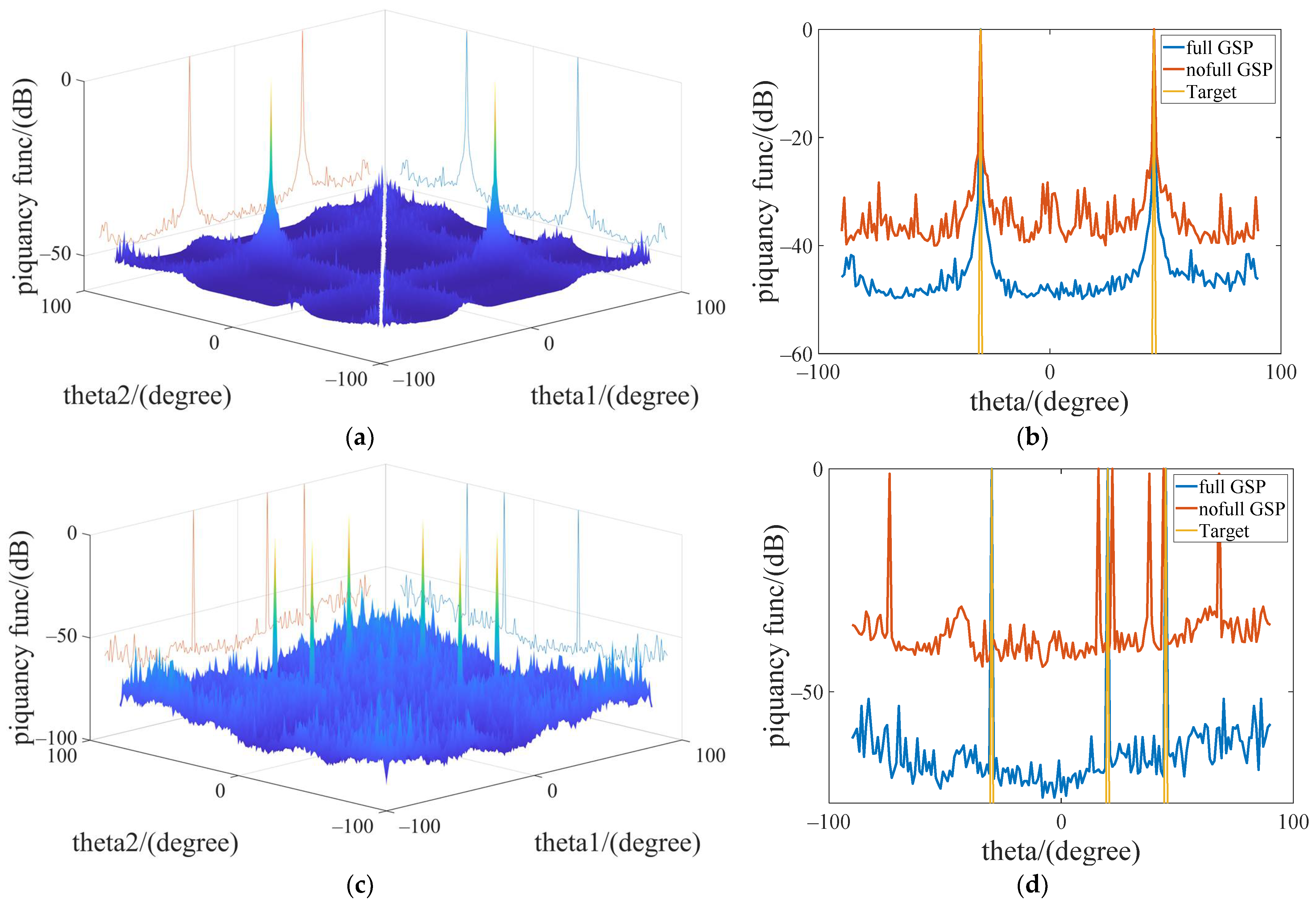
Figure 4 shows the result response results of the graph signal azimuth to the dual and multi-target estimation. Figure 4b,d are the dimensionality reduction plan views of Figure 4a,c, respectively. The blue curve is the result of the azimuth estimation of the full GSP algorithm; the red curve is the result of the estimation of the nofull GSP algorithm according the previous work [23]; and the yellow curve is the original azimuth parameter. From Figure 4b of the dual target estimation, it can be seen that the blue line represented by the fully GSP can achieve the −3 db sidelobe effect at the −40 db response strength and can accurately estimate the target point { 30 ° , 45 ° } ; compared with the red line of the nofull GSP algorithm, the full GSP has lower side lobes and more accurate results. From Figure 4d of the multi-target estimation, it can be seen that the full GSP can also accurately estimate the azimuth parameters of the target point { 45 ° , 20 ° , 30 ° } . At this time, the F GSP ( θ i ) of nofull GSP has been incorrectly estimated, which proves that the full GSP algorithm is better in azimuth than the nofull GSP algorithm.
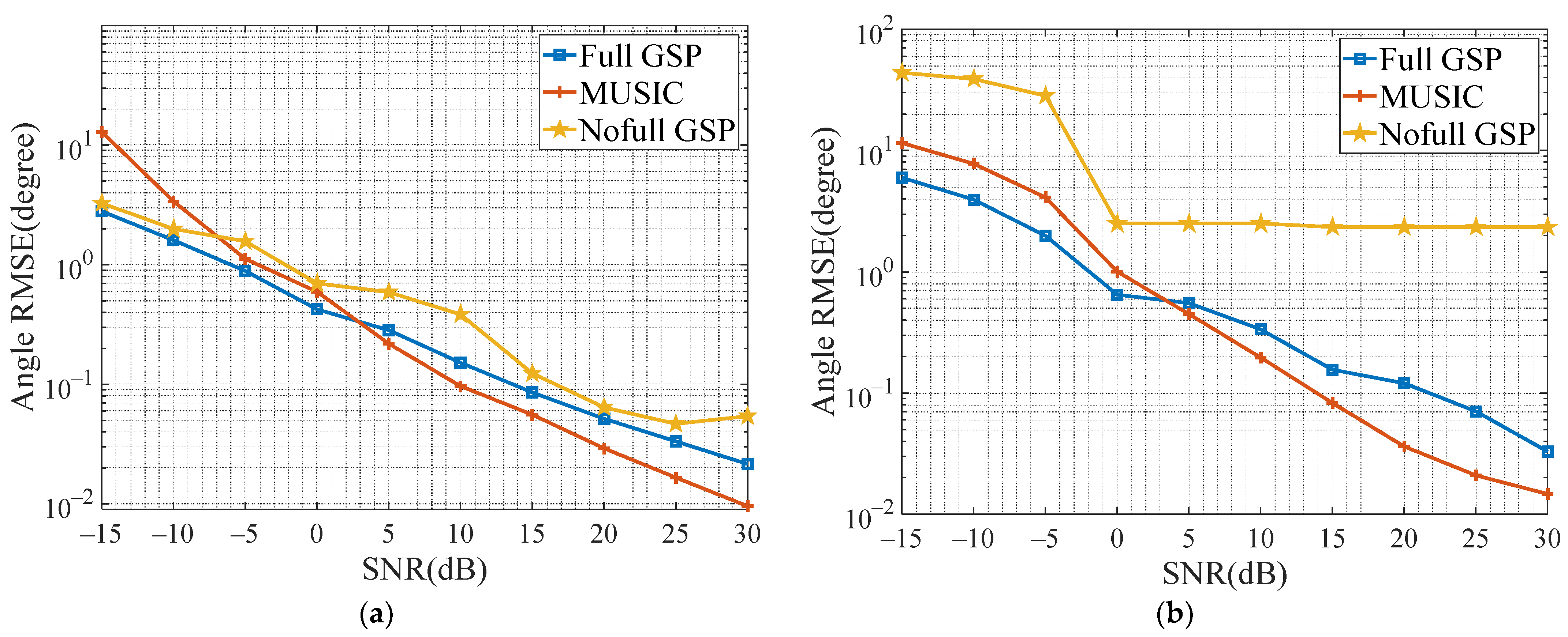
The experiment also carried out Monte Carlo analysis 500 times to analyze the influence of the signal-to-noise ratio of the azimuth estimation performance. For further comparison and analysis, the experiment quoted the classic MUSIC estimation algorithm [27]. It can be seen in Figure 5a that when the signal-to-noise ratio is lower than 0 dB, the signals of both full GSP and nofull GSP algorithm are better than MUSIC performance of the algorithm; in Figure 5b, it can be seen that because of the complexity of multi-target estimation algorithm, we set the search boundary under high SNR. Experiments show that the nofull GSP algorithm cannot accurately estimate the multi-target, and the search results appear on the search boundary or even exceed the boundary; the fully GSP algorithm still shows better performance than the MUSIC algorithm when the SNR is lower than 0 dB.

3.2. Distance Estimation Results and Monte Carlo Analysis

For the distance estimation situation, considering a single radar array element emitting N f = 8 frequency point signals to form a bandwidth signal, the experimental scene is that near-field dual-targets are located at { 9750   m , 10,040   m } , and near-field multi-targets are located at { 9650   m , 10,050   m , 10,200   m } .
Figure 6 shows the results of the estimated signal distance to the dual-target and multi-target estimation. From Figure 6b of dual-target estimation, it can be seen that the full GSP can still accurately estimate the distance parameter to the target point { 9750   m , 10,040   m } , However, the nofull GSP algorithm has been unable to estimate the distance of double targets, and the response function F GSP ( R i ) has been unable to find the accurate maximum value. From Figure 6d of multi-target estimation, it can be seen that the full GSP algorithm can also accurately estimate the distance parameters { 9650   m , 10,050   m , 10,200   m } ; but for the nofull GSP algorithm, its F GSP ( R i ) has a corresponding mean value similar to Gaussian white noise. Experiments show that the full GSP algorithm can also achieve the distance estimation. Next, the full GSP algorithm is analyzed by Monte Carlo experiment and compared with the performance of MUSIC algorithm.
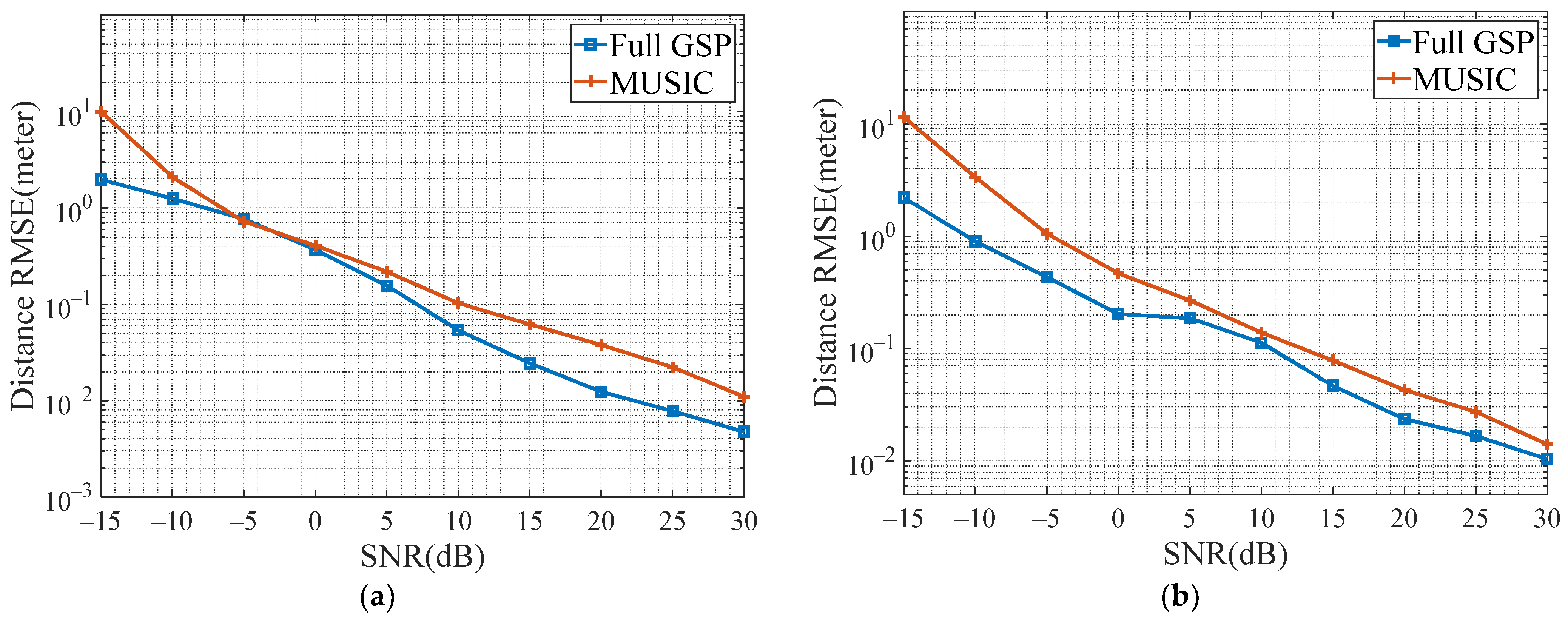
The distance estimation has also undergone 500 Monte Carlo analysis. Considering that the nofull GSP algorithm cannot perform the distance estimation, only the result of the full GSP and the MUSIC algorithm is compared here. As can be seen from Figure 7a,b, full GSP algorithm is better than the MUSIC algorithm under any SNR condition, and the estimation result is more accurate. The specific reasons will be analyzed in Section 4.

3.3. Joint Estimation Results

Finally, for the case of joint estimation, consider a radar array composed of M = 8 collocated transceiver antennas. Each array element transmits Δ f frequency interval signals to form a broadband signal. Under the 30 dB SNR condition, experiment scene 1 is single-target estimation, and the target parameter is { 42 ° , 9900   m } ; experiment scene 2 is multi-target estimation, and the target parameter is { 30 ° , 10,200   m } , { 45 ° , 9750   m } . The rest of the conditions are the same as the above experiment.
Figure 8 shows the result of the joint estimation for single target. It can be seen from Figure 8a that the full GSP algorithm can accurately estimate the azimuth and distance parameters to the target point. The target point’s parameters { 42 ° , 9900   m } is less than or equal to −35 dB, achieving good two-dimensional estimation results. Experiments have also proved that the graph signal method has good response results in azimuth, distance, and joint estimation. Figure 8b shows the slice diagram of the full GSP estimation algorithm in azimuth and distance dimension. Since F GSP ( θ i , R ) . * F GSP ( θ , R i ) will only produce one target point under single target joint estimation and will not produce false points, the next experiment shows multi-target joint estimation and CLEAN algorithm to eliminate false points.
Figure 9 shows the result of joint estimation of azimuth and distance for multi-point target. It can be seen from Figure 9a that the fully connected graph signal can perform accurate joint estimation of the azimuth and distance for multi-target points, but there will be the false target point phenomenon, and as shown in the figure, the target points { 30 ° , 9750   m } , { 45 ° , 10,020   m } are false, which is related to the graph signal solving algorithm itself. The sidelobe value near the target point parameter { 30 ° , 10,020   m } , { 45 ° , 9750 m } is less than or equal to −35 dB, achieving a good two-dimensional estimation result. It can be seen that in the case of multiple targets, false points will appear, which need to be processed through the CLEAN algorithm, and the false points are eliminated through the construction of the Point Spread Function to obtain the correct result.
Figure 10 shows the results of eliminating false points in the complete GSP joint estimation results using the CLEAN algorithm according to Algorithm 3. In the process of clean algorithm, Figure 10a is the normalized response diagram of joint estimation of graphic signals after using CLEAN algorithm. It can be seen that CLEAN algorithm retains the distance and phase information of real point targets and eliminates false points accurately. Figure 10b is a sectional view of the azimuth and distance of the GSP algorithm. It can be seen that the fully connected map signal can accurately estimate the azimuth and distance information of multiple targets.

4. Discussion

In this Section, we will discuss and analyze the estimation principle and simulation results of GSP, which include the performance analysis and the principle interpretation of various algorithms; discussion on the nofull GSP, GSP and MUSIC algorithm complexity and computational load comparison; and discussion on the solution of unknown estimated target number k .

4.1. Results and Performance Analysis of GSP Estimation Method

In Figure 5 and Figure 7, we have done 500 Monte Carlo experiments on the azimuth estimation and distance estimation respectively, and compared the accuracy of GSP, Nofull GSP and music algorithm.
In the azimuth estimation experiment, we can observe that GSP algorithm is better than Nofull GSP algorithm in any SNR condition, because GSP algorithm build the adjacency matrix A θ R by using the phase relationship between all array elements, so when the search domain parameters I are aligned with the target I , the graph Fourier operator Q A forms the same linear phase relationship with the echo signal X r e c , which satisfies Equation (27). At this time, the I maximum eigenvalues of the graph Fourier operator Q A correspond to the I targets of the echo signal, Therefore, GSP algorithm show better performance than Nofull GSP algorithm.
We can also observe that the performance of GSP algorithm is not as good as MUSIC algorithm when the SNR is greater than 0, because GSP algorithm uses the form of 2 π f when constructing the steering vector, and in the distance search domain θ i I under far-field conditions, the ratio of the numerator denominator of the exponential term of the guidance vector Equation (17) will approach a variable that changes greatly θ i with, as shown below:
e j 2 π f 2 ( m 1 ) d sin ( θ i ) c f ( θ i )
which makes the elements of the adjacency matrix A θ R prone to periodic repetition, and the linear relationship between Q A and X r e c of echo signal after graph Fourier transform is weakened, resulting in the poor performance of GSP algorithm than MUSIC algorithm under high SNR condition.
In the distance estimation experiment, because the nofull GSP algorithm has been unable to estimate the information about distance, we only compare the performance of GSP and MUSIC algorithm. It can be observed that GSP algorithm is better than MUSIC algorithm in the any SNR condition, because in the distance estimation, GSP algorithm uses the form of Δ f when constructing the steering vector, while in the distance search domain R i I under far-field conditions, the proportion of the numerator denominator of the exponential term of the guidance vector Equation (19) will approach a small constant C , as shown below:
e j 2 π m Δ f ( 2 R i c ) C
This small constant C avoids the periodic repetition of the elements of the adjacency matrix A θ R , making it easier for the graph Fourier operator Q A to form the same linear phase relationship with the echo signal X r e c ; Moreover, GSP algorithm constructs an adjacency matrix on I search dimensions to estimate the target. Compared with one search estimation of MUSIC algorithm, GSP algorithm has better orthogonality to the signal subspace Q S and noise subspace Q N . At the same time, graph Fourier operator Q A can better fit the accurate information of multi targets. Therefore, in distance estimation, GSP algorithm performs better than MUSIC algorithm under the condition of any SNR; At the same time, the construction of multiple search dimensions of GSP algorithm can ensure that the signal subspace Q S and noise subspace Q N are still orthogonal under the low SNR condition, which also explains that the performance of GSP algorithm is better than MUSIC algorithm in the case of low SNR in azimuth estimation.
The Monte Carlo experimental data results of azimuth and range algorithms are shown in Table 1 and Table 2. From Table 1, it can be seen that in azimuth estimation, the performance of GSP algorithm is better than that of nofull GSP algorithm under the condition of any SNR; When the SNR is lower than 0 dB, the performance of GSP algorithm is better than MUSIC algorithm. It can be seen from Table 2 that in distance estimation, GSP algorithm has better performance than MUSIC algorithm under the condition of any SNR.
As we can see from Table 3, in azimuth estimation, GSP algorithm has 45.6% performance improvement compared with MUSIC algorithm under the condition of low SNR; In distance estimation, GSP algorithm has 47.4% performance improvement compared with music algorithm under the condition of any SNR.

4.2. Analysis of Time Complexity and Computational Load

According to Section 4.1, the characteristic of GSP algorithm is that when the search domain I is aligned with the target parameters, it will get a huge response value; It can be seen from Algorithm 1, the solution process of GSP algorithm includes solving the element value of the adjacency matrix A C N * N ; solving the eigenvector of the adjacency matrix according to Equation (29); removing I maximum values and solving the response function F GSP (32), and the above processes are completed iteratively in the search domain grid G = 100 ; The solution process of nofull GSP and GSP algorithm is exactly the same, except for a little difference in the process of graph modeling. Therefore, the computational complexity of nofull GSP algorithm is the same as GSP, and their computational complexity is deduced as follows:
(1)
Computing the element of the adjacency matrix A θ R by the received signal X r e c is O ( N * ( N 1 ) ) .
(2)
Computing the EVD of adjacency matrix A θ R is O ( N 3 ) .
(3)
Sort Q A X r e c , and delete the maximum value of the first I items, then counting down to get the response value result F GSP is O ( N * I + 1 ) .
(4)
The above process is about the iteration of the I -th power of the search domain G , and its algorithm complexity is O ( G I ) .
Therefore, the algorithm complexity of nofull GSP and GSP algorithm is
O ( GSP ) = O ( nofullGSP ) = O ( G I * ( N 3 + N 2 + ( I 1 ) N + 1 ) ) ~ O ( G I N 3 )
From the above analysis, it can be seen that the full GSP algorithm constructs the search domain I and uses the increased computing cost to improve the performance of the estimation algorithm, which is indeed a defect in the design of the full GSP algorithm.
And the solution process of MUSIC algorithm includes: solving the covariance matrix R xx ; solving the eigenvector of the covariance matrix R xx ; removing I maximum values, then solving the noise subspace Q S and calculating the response value F M U S I C . The above processes are completed iteratively in the search domain grid G = 100 . Therefore, the computational complexity of MUSIC algorithm is deduced as follows:
(1)
Computing the covariance matrix R xx by the received signal X r e c is O ( N 2 ) .
(2)
Computing the EVD of the covariance matrix R xx is O ( N 3 ) .
(3)
Sort R xx , and delete the maximum value of the first I items, solving the noise subspace Q S and calculating the response value F M U S I C is O ( N * I + 2 ) .
(4)
The above process is about the iteration of search domain G , and its algorithm complexity is O ( G ) .
O ( MUSIC ) = O ( G * ( N 3 + N 2 + NI + 2 ) ) ~ O ( GN 3 )
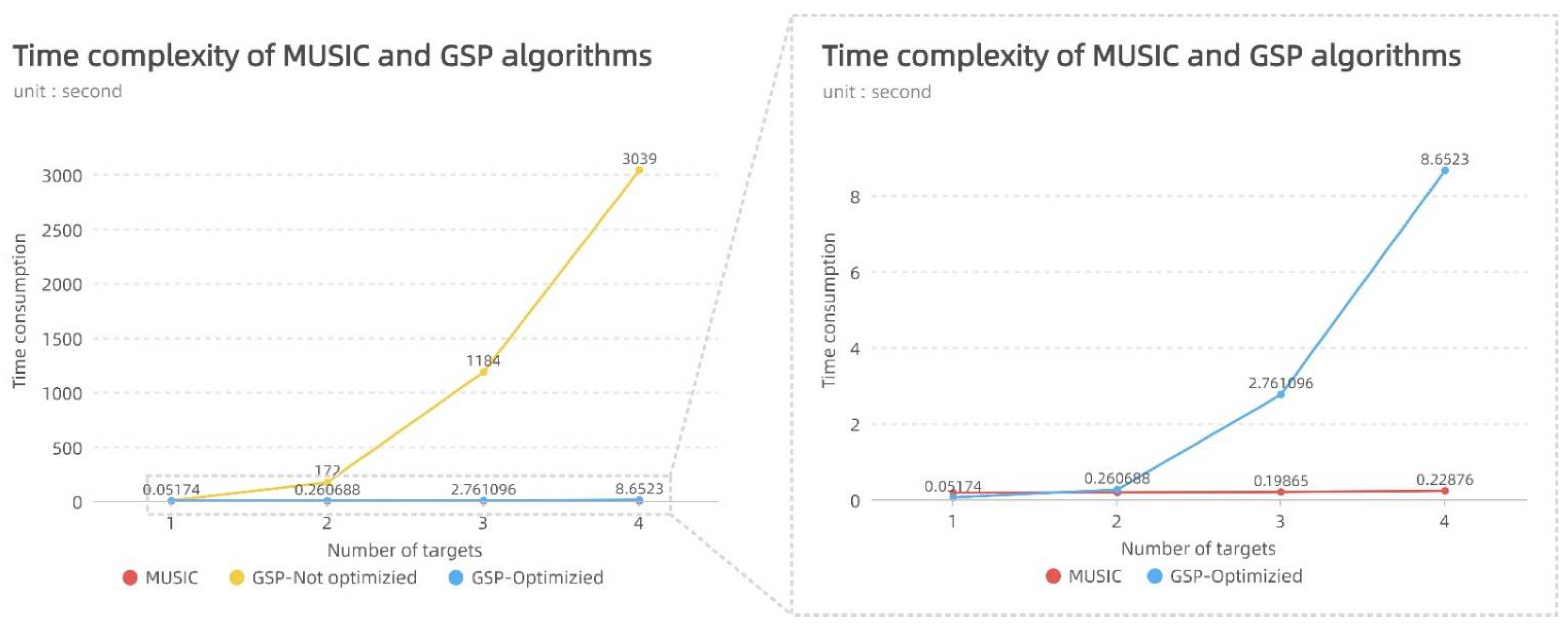
By comparing Equations (36) and (37), it can be seen that the algorithm complexity of nofull GSP and GSP algorithm includes the high-order power O ( G I ) of the search grid, so their computational complexity mainly depends on the establishment and traversal of the search element domain G (related to the number of targets I ). When the number of targets I increases, the increase of computation will be exponential, Therefore, the complexity of nofull GSP and GSP algorithm without parallel optimization is worse than MUSIC algorithm, the complexity of these algorithms is shown in Table 4 as below:
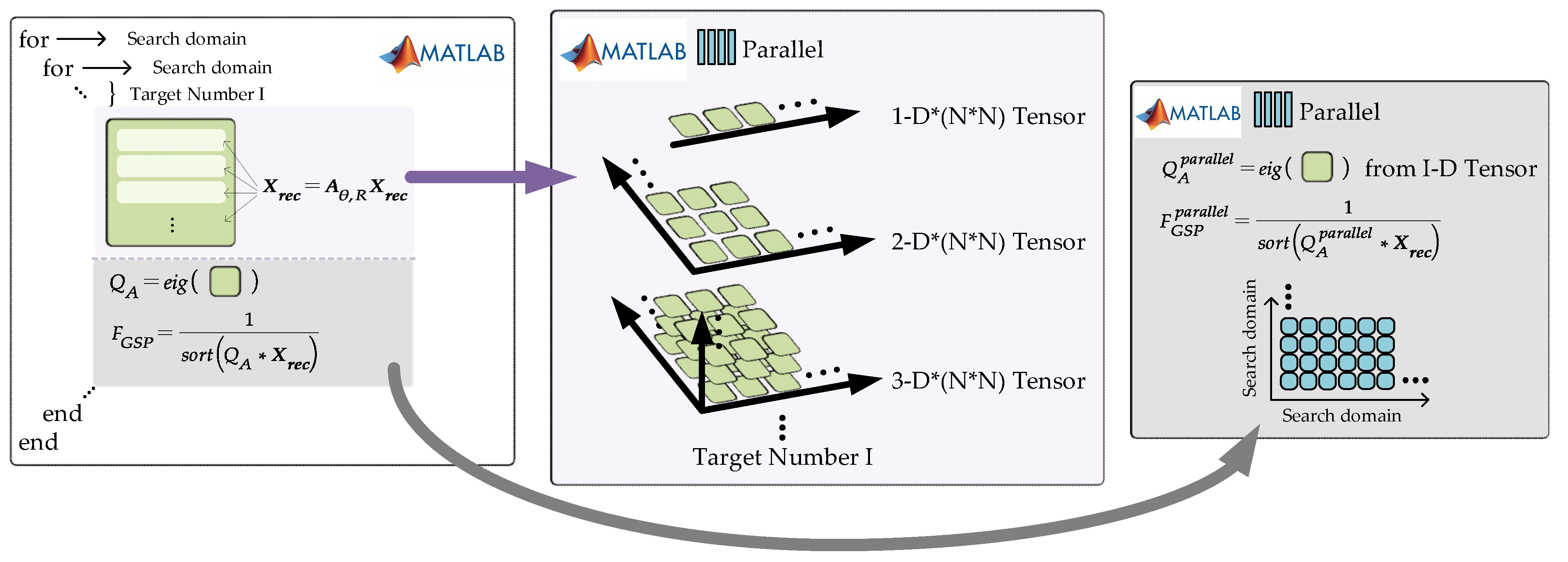
Therefore, we need to speed up the GSP and nofull GSP algorithm through the scheme of parallel computing to reduce the computing load and eliminate the influence of O ( G I ) . It can be seen that the search domain I will produce a large number of core algorithm processes, which will show a great computational load in the process of serial operation. Fortunately, this large-scale small matrix is very suitable for parallel acceleration. We can greatly improve the computing speed of GSP and nofull GSP algorithm and reduce the computing time of GSP and nofull GSP algorithm by constructing the high-dimensional tensor of adjacency matrix and making it into a data form suitable for MATLAB parallel accelerated computing. The schematic diagram of MATLAB parallel computing acceleration is shown in Figure 11 as below:
In this experiment, AMD Ryzen 3600× processor and 32 g memory are used for accelerated experimental simulation under Windows10 system. The unoptimized GSP algorithm, optimized GSP algorithm and MUSIC algorithm are based on the condition that the search domain gird is 100. The results are as follows:
As can be seen from Figure 12, under the search grid setting of G = 100 , the operation time of the optimized GSP and nofull GSP algorithm is 465 times faster than that of the unoptimized GSP and nofull GSP algorithm, which is close to the MUSIC algorithm. Thanks to the support of MATLAB for tensor parallel computing, O ( G I ) in the complexity of nofull GSP and GSP algorithm can be approximately regarded as the lower order term of O ( G ) , which reduces the computational load of nofull GSP and GSP algorithm to an acceptable range.

4.3. Estimation Method of Unknown Target Number K

In the experiment in Section 3, we all carry out verification simulation and a performance test on the GSP algorithm assuming that the number of targets I is known. However, in the actual scene, we could not know the number of specific targets I , so we need to conduct experimental analysis when the number of targets I is unknown.
Firstly, the Unknown Number of Source Estimation and Blind Signal Estimation is a key problem in the field of Array Signal Processing. Without the number of targets, it is impossible to further measure and estimate the targets. For the typical target parameter estimation problem, when the number of targets should be known or the number of targets K should be obtained through the Blind Signal Estimation algorithm in advance, the target parameters should be further estimated and measured. In the field of Blind Signal Estimation, the basic idea of source number estimation is to calculate the covariance matrix R xx ( n ) through the echo signal x ( n ) . By solving the SVD eigenvalues of the covariance matrix, the larger K eigenvalues in the eigenvalues are accumulated to estimate the number of sources K [28,29,30].
Secondly, we can know from the general solving algorithm of graph signal in Section 2.4.2 that when we calculate the eigen decomposition of adjacency matrix A , the target number I maximum eigenvalues will be generated. It should be noted that the number of maximum eigenvalues does not depend on the preset K , but depends on the number of actual targets I , which means that when the number of search variables K in the search area increases to the number of actual targets I , there will be I maximum eigenvalues generated, what we need to do is to increase the number of search variables K . To sum up, the full GSP algorithm can indeed estimate the size of the real K by increasing the number of K while the number of targets K is unknown, but this process is the inverse process of the Unknown Number of Source Estimation algorithm. The experimental results can only verify that the full GSP algorithm has the characteristics of estimating the number of targets K but cannot verify that the GSP algorithm is a necessary condition of the Unknown Number of Source Estimation algorithm.
For the case of unknown target number I , the model Equation (6) needs to be modified as follows:
X = C B T S + W
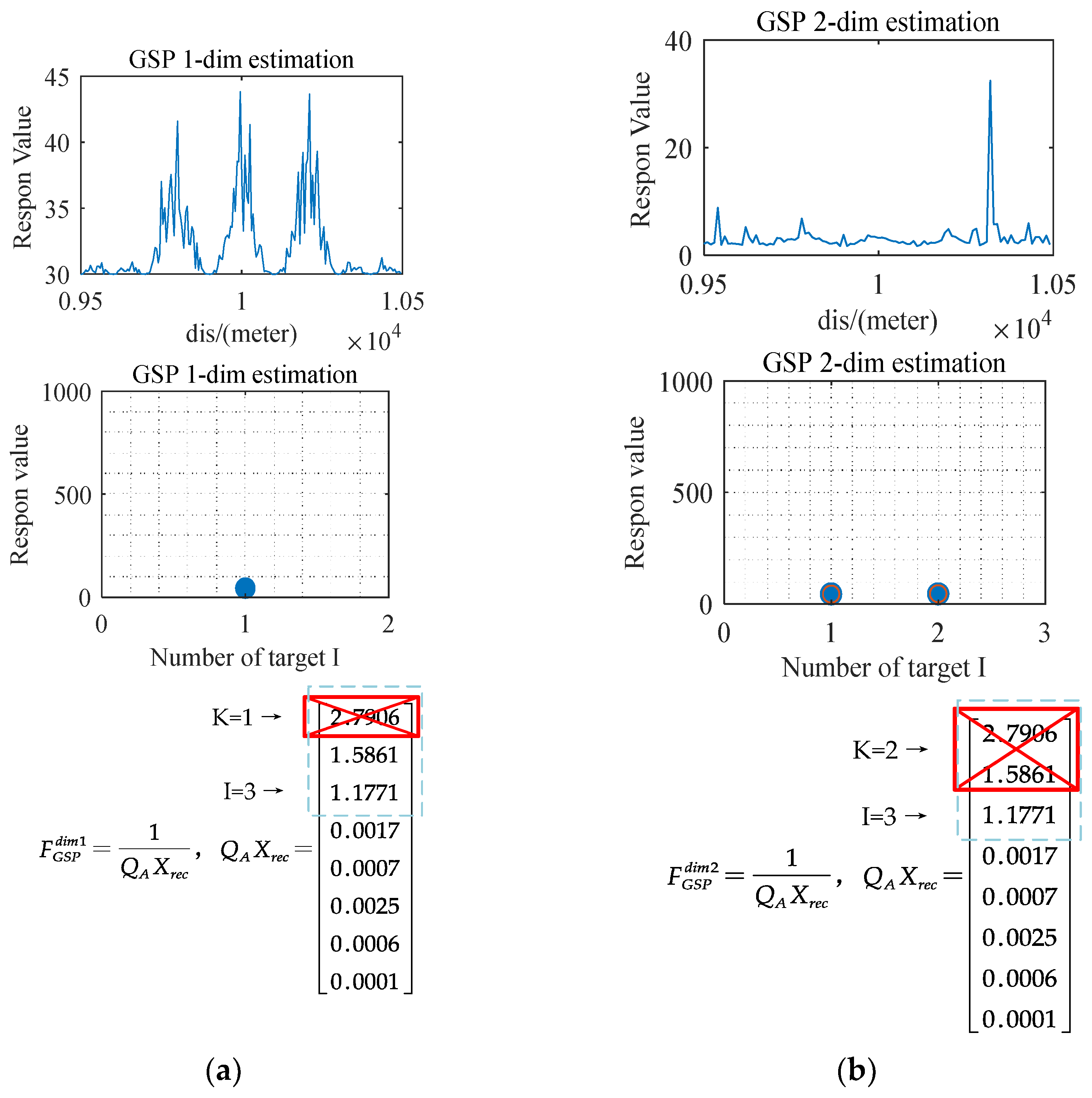
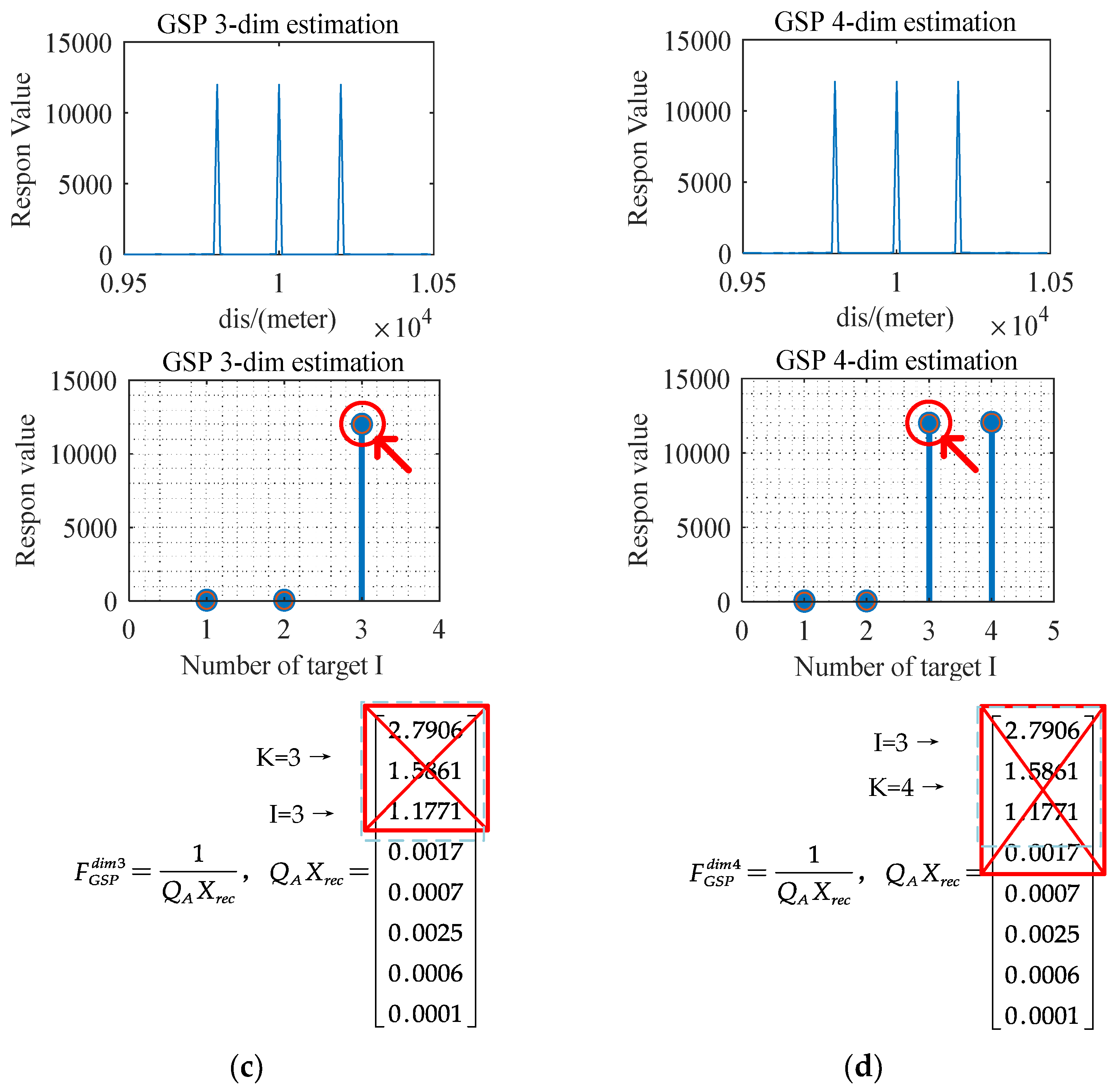
The received signal X r e c form of unknown target number K is generated through the above formula. Assuming that the current estimated target number is K , GSP estimation experiment is carried out. All conditions of this experiment are the same as those in Section 3, Figure 13 shows the response results, judgment threshold and algorithm principle of GSP algorithm under different target number K as below:
We discuss different situations for different estimated number k as below:
1.
When the estimates number K < I , the search domain of GSP algorithm is K , and F GSP function will not have sharp peaks and will cause confusion in the estimation results. As shown in Figure 13a,b, the response of the search result is very small. This is because even if the parameter K of the search domain is aligned with any K in the target I , I maximum eigenvalues will appear as long as K < I . and deleting the eigenvalues of the first K large numbers in Q A X rec will not make F GSP have a huge response value, so it is impossible to obtain accurate estimation when K < I .
2.
When the estimated number K = I , the search domain of GSP algorithm K is equal to I , F GSP function will produce K sharp peaks, and the size of each spike is greater than 10e4. At this time, it can be preliminarily determined that the estimated number of targets is K . As shown in Figure 13c, the searched parameter K is equal to the actual number of targets I , resulting in I large eigenvalues. Therefore, when K = I , deleting K eigenvalues will make Q A X rec produce a huge response. At this time, it can be preliminarily determined that K is the target number.
3.
When the estimated number K > I , the search domain of GSP algorithm K has one more dimension than I , the F GSP function will also only produce I spikes, and no matter how the K value is increased, the F GSP response result remains unchanged. At this time, it can be determined that the estimated target is I . As shown in Figure 13d, at this time, the parameter K of the search domain is aligned with the target I , whether the remaining K I dimension is aligned with the target or not, it will only make Q A X rec produce I maximum values. At this time, even deleting the first K maximum values will not affect the estimation results F GSP , because the remaining eigenvalues have nothing to do with the target parameters, even if deleted, it can still produce a huge corresponding effect on. At this time, it can be determined that the previously estimated K is the target number I .

5. Conclusions

In this article, a joint estimation method based on graph signal for far-field targets was proposed, and a general solution to the problem of graph signal estimation was given. The proposed method constructs a fully connected graph signal matrix through the radar array model and archives the azimuth and distance joint estimation with sufficient estimation accuracy. In this article, the derivation and analysis showed that the estimation method based on fully connected graph signal makes full use of the phase information between array elements and has better performance than nofull GSP algorithm and MUSIC algorithm. The experimental results show that, in azimuth estimation, the GSP algorithm has a 45.6% performance improvement compared with the MUSIC algorithm under the condition of low SNR. In distance estimation, the GSP algorithm has 47.4% performance improvement compared with the MUSIC algorithm under the condition of any SNR under the far-filed conditions. Numerical experiments show that the GSP algorithm is superior to the MUSIC algorithm, because it exchanges the computational load for the improvement of algorithm performance.
For the problem of computational load, the unoptimized GSP algorithm shows a huge computational load in computational complexity. The main reason is that the construction of the search domain of GSP algorithm leads to exponential terms in its computational complexity. Through MATLAB parallel computing acceleration experiment, it was proved that the speed of the optimized GSP algorithm was increased by 465 times, which greatly improves the engineering applicability of the GSP algorithm. In the future, our work will focus on the accelerated application of GSP algorithm in Spark distributed computing framework.
For the assumption that the target number k of GSP algorithm is unknown, we drew a conclusion through theoretical derivation and experimental analysis: when the number of targets K is unknown, we can estimate the K dimension by gradually increasing the search domain K . If the current response value is less than 10e4, continue to increase the K value to estimate the next search domain. If the current response value is greater than 10e4, and further increasing the K value will not affect the size of the response value, it can be considered that the K with the first response value reaching 10e4 is the number of real targets I .

Author Contributions

K.L. and J.J. conducted the algorithm design; Z.Y. and N.X. made a MATLAB implementation of the proposed algorithm and formulated the proposed algorithm. Z.Y. contributed to prepare and analyze the experimental data and the results. All authors were involved in modifying the article, the literature review, and the discussion of the results. All authors have read and agreed to the published version of the manuscript.

Funding

This work was Supported by National Natural Science Foundation of China (61871425), Natural Science Foundation of Guangxi (2021GXNSFAA220051), Guangxi special fund project for innovation-driven development (GuikeAA21077008), Guangxi Key Laboratory of Wireless Wideband Communication and Signal Processing.

Institutional Review Board Statement

Not applicable.

Informed Consent Statement

Not applicable.

Data Availability Statement

Not applicable.

Acknowledgments

We thank all editors and reviewers and for their valuable comments and suggestions for improving this manuscript.

Conflicts of Interest

The authors declare no conflict of interest.

References

  1. Xu, T.; Wang, X.; Huang, M.; Lan, X.; Sun, L. Tensor-Based Reduced-Dimension MUSIC Method for Parameter Estimation in Monostatic FDA-MIMO Radar. Remote Sens. 2021, 13, 3772. [Google Scholar] [CrossRef]
  2. Weiss, S.; Alrmah, M.; Lambotharan, S.; McWhirter, J.; Kaveh, M. Broadband Angle of Arrival Estimation Methods in a Poly-nomial Matrix Decomposition Framework. In Proceedings of the 2013 5th IEEE International Workshop on Computational Advances in Multi-Sensor Adaptive Processing (CAMSAP), St. Martin, France, 15–18 December 2013. [Google Scholar]
  3. Li, L.; Yao, J.; Liu, Y.; Yuan, W.; Shi, S.; Yuan, S. Optimal Seamline Detection for Orthoimage Mosaicking by Combining Deep Convolutional Neural Network and Graph Cuts. Remote Sens. 2017, 9, 701. [Google Scholar] [CrossRef] [Green Version]
  4. Moreira, L.A.S.; Ramos, A.L.L.; de Campos, M.L.R.; Apolinario, J.A.; Serrenho, F.G. A Graph Signal Processing Approach to, Direction of Arrival Estimation. In Proceedings of the 2019 27th European Signal Processing Conference (EUSIPCO), A Coruna, Spain, 2–6 September 2019. [Google Scholar] [CrossRef]
  5. Proudler, I.K.; Stankovic, V.; Weiss, S. Narrowband Angle of Arrival Estimation Exploiting Graph Topology and Graph Signals. In Proceedings of the 2020 Sensor Signal Processing for Defence Conference (SSPD), Edinburgh, UK, 15–16 September 2020; pp. 1–5. [Google Scholar] [CrossRef]
  6. Raia, T.C.; Thomas, M.G.P.; Serrenho, F.G.; Apolinário, J.A., Jr. GSP-based DoA estimation for a multimission radar. In Proceedings of the XXXVIII Simpósio Brasileiro de Telecomunicações e Processamento de Sinais (SBrT2020), Florianopolis, Brazil, 22–25 November 2020. [Google Scholar]
  7. Jiang, L.; Cheng, M.; Matsumoto, T. A TOA-DOA Hybrid Factor Graph-Based Technique for Multi-Target Geolocation and Tracking. IEEE Access 2021, 9, 14203–14215. [Google Scholar] [CrossRef]
  8. Weisberg, K.; Laufer-Goldshtein, B.; Gannot, S. Simultaneous Tracking and Separation of Multiple Sources Using Factor Graph Model. IEEE ACM Trans. Audio, Speech, Lang. Process. 2020, 28, 2848–2864. [Google Scholar] [CrossRef]
  9. Alcantara, E.; Atlas, L.; Abadi, S. Direction-of-Arrival Estimation Using Signal Processing on Graphs. In Proceedings of the 2021 IEEE Statistical Signal Processing Workshop (SSP), Rio de Janeiro, Brazil, 11–14 July 2021; pp. 1–5. [Google Scholar] [CrossRef]
  10. Ortega, P.A.; Frossard, J.; Kovačević, J.M.F.; Moura, P. Vandergheynst. Graph Signal Processing: Overview, Challenges, and Applications. Proc. IEEE 2018, 106, 808–828. [Google Scholar] [CrossRef] [Green Version]
  11. Alcantara, E.; Atlas, L.; Abadi, S. Applying concepts and tools from signal processing on graphs (SPG) to problems in array signal processing. J. Acoust. Soc. Am. 2018, 143, 1852. [Google Scholar] [CrossRef]
  12. Sandryhaila, A.; Moura, J.M.F. Discrete signal processing on graphs: Graph fourier transform. In Proceedings of the 2013 IEEE International Conference on Acoustics, Speech and Signal Processing, Vancouver, BC, Canada, 26–31 May 2013; pp. 6167–6170. [Google Scholar] [CrossRef]
  13. Xiong, C.; Fan, C.; Huang, X. Time Reversal Linearly Constrained Minimum Power Algorithm for Direction of Arrival Esti-mation in Diffuse Multipath Environments. Remote Sens. 2020, 12, 3344. [Google Scholar] [CrossRef]
  14. Schwarz, U.J. Mathematical-statistical Description of the Iterative Beam Removing Technique (Method CLEAN). Astron. Astrophys. 1978, 65, 345–356. [Google Scholar]
  15. Van Trees, H.L. Optimum Array Processing; Part IV of Detection, Estimation, and Modulation Theory, Detection, Estimation, and Modulation Theory; Wiley: Hoboken, NJ, USA, 2004; pp. 154–196. [Google Scholar] [CrossRef]
  16. Nion, D.; Sidiropoulos, N. Tensor Algebra and Multidimensional Harmonic Retrieval in Signal Processing for MIMO Radar. IEEE Trans. Signal. Process. 2010, 58, 5693–5705. [Google Scholar] [CrossRef]
  17. Scharf, L.; Friedlander, B. Matched subspace detectors. IEEE Trans. Signal. Process. 1994, 42, 2146–2157. [Google Scholar] [CrossRef] [Green Version]
  18. Zhang, R.; Xu, K.; Quan, Y.; Zhu, S.; Xing, M. Signal Subspace Reconstruction for DOA Detection Using Quantum-Behaved Particle Swarm Optimization. Remote Sens. 2021, 13, 2560. [Google Scholar] [CrossRef]
  19. Leskovec, L.; Chakrabarti, D.; Kleinberg, J.; Faloutsos, C.; Ghahramani, Z. Kronecker graphs: An ap-proach to modeling networks. J. Mach. Learn. 2010, 11, 985–1042. [Google Scholar]
  20. Dudgeon, D.E.; Mersereau, R.M. Discrete-Time Signal. Processing; Prentice Hall: Hoboken, NJ, USA, 1983; pp. 1–3. [Google Scholar]
  21. Hellmuth, M.; Merkle, D.; Middendorf, M. Extended shapes for the combinatorial design of RNA sequences. Int. J. Comput. Biol. Drug Des. 2009, 2, 371–384. [Google Scholar] [CrossRef] [PubMed]
  22. Sandryhaila, A.; Moura, J.M. Big Data Analysis with Signal Processing on Graphs: Representation and processing of massive data sets with irregular structure. IEEE Signal. Process. Mag. 2014, 31, 80–90. [Google Scholar] [CrossRef]
  23. Xiao, P.; Xu, L.; Xu, L. Graph-based Matched Field Localization for an Underwater Source. arXiv 2010, arXiv:2101.07137. [Google Scholar]
  24. Schmidt, R.O. A Signal. Subspace Approach to Multiple Emitter Location and Spectral Estimation; Stanford University: Stanford, CA, USA, 1982; pp. 10–14. [Google Scholar]
  25. Morency, M.W.; Vorobyov, S.A.; Leus, G. Joint Detection and Localization of an Unknown Number of Sources Using the Algebraic Structure of the Noise Subspace. IEEE Trans. Signal. Process. 2018, 66, 4685–4700. [Google Scholar] [CrossRef] [Green Version]
  26. He, P.; Chen, B.; Yang, M. A novel sidelobe suppression method based on the CLEAN algorithm for bi-phase codes pulse compression. In Proceedings of the 2016 CIE International Conference on Radar (RADAR), Guangzhou, China, 10–13 October 2016; pp. 1–4. [Google Scholar] [CrossRef]
  27. Odendaal, J.W.; Barnard, E.; Pistorius, C.W.I. Two-dimensional Super-resolution radar imaging using the MUSIC algorithm. IEEE Trans. Antennas Propag. 1994, 42, 1386–1391. [Google Scholar] [CrossRef]
  28. Zhi, Q.; Zi, H.; Man, C. A method for signal source number estimation based on MUSIC algorithm. In Proceeding of the 2015 IEEE International Conference on Communication Problem-Solving (ICCP), Guilin, China, 16–18 October 2015; pp. 344–346. [Google Scholar]
  29. Istenic, R.; Zazula, D. Estimation of the Number of Signal Sources in Compound Signals Using Activity Index Variance. In Proceedings of the 2009 IEEE 13th Digital Signal Processing Workshop and 5th IEEE Signal Processing Education Workshop, Marco Island, FL, USA, 4–7 January 2009; pp. 178–181. [Google Scholar]
  30. Liu, L.; Yang, X.; Gao, S.; Li, S. Source Number and DOA Estimation Method Based on Eigen-Beam MUSIC for Closely Spaced Signals. In Proceedings of the 2019 IEEE International Conference on Signal, Information and Data Processing (ICSIDP), Chongqing, China, 11–13 December 2019; pp. 1–5. [Google Scholar]
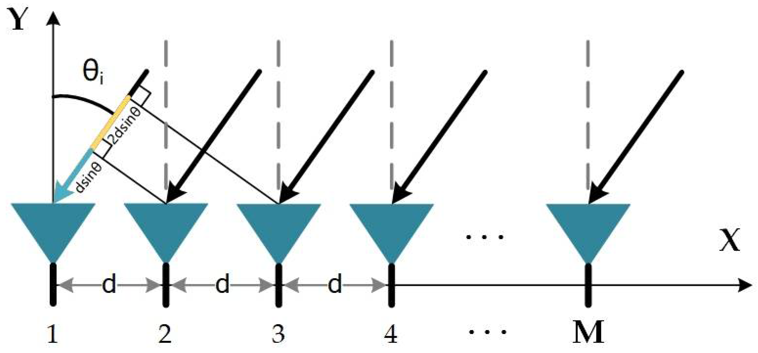
Figure 1. Radar array signal model.
Remotesensing 14 01110 g001
Figure 2. Radar array joint estimation model.
Remotesensing 14 01110 g002
Figure 3. Graphic signal model of stepped frequency radar array.
Remotesensing 14 01110 g003
Figure 4. GSP azimuth estimation response map with dual and multi-target experiments in 30 db SNR. (a) Dual-target estimation results. (b) Estimation result comparison. (c) Multi-target estimation results. (d) Estimation result comparison.
Remotesensing 14 01110 g004
Figure 5. Results of 500 Monte Carlo azimuth estimation experiments of three algorithms (a) Two-target estimation results. (b) Multi-target estimation results.
Remotesensing 14 01110 g005
Figure 6. GSP distance estimation response map with dual and multi-target experiments in 30 db SNR (a) Dual-target distance estimation. (b) Estimation result comparison. (c) Multi-target distance estimation. (d) Estimation result comparison.
Remotesensing 14 01110 g006
Figure 7. Results of 500 Monte Carlo distance estimation experiments of the two algorithms. (a) Two-target distance estimation results. (b) Three-target distance estimation results.
Remotesensing 14 01110 g007
Figure 8. GSP Joint estimation of azimuth and distance estimation results (a) azimuth and distance dimensional response map (b) slice diagram of response map.
Remotesensing 14 01110 g008
Figure 9. GSP Joint estimation of azimuth and distance results for multi-targets (a) azimuth and distance dimensional response map (b) slice diagram response map.
Remotesensing 14 01110 g009
Figure 10. GSP CLEAN algorithm eliminates the false point of the graph signal joint estimation result. (a) CLEAN algorithm normalization results. (b) CLEAN algorithm azimuth and distance slice map.
Remotesensing 14 01110 g010
Figure 11. Principle of GSP algorithm Tensor construction and parallel computing.
Remotesensing 14 01110 g011
Figure 12. Time complexity comparison result of MUSIC and GSP and unoptimized GSP algorithm.
Remotesensing 14 01110 g012
Figure 13. Experiment result including response value map, response peak map, eigenvalue deletion of GSP algorithm with unknown target number K. (a) K = 1 within one dimensional estimation. (b) K = 2 within two dimensional estimation. (c) K = 3 within three dimensional estimation. (d) K = 4 within four dimensional estimation.
Remotesensing 14 01110 g013aRemotesensing 14 01110 g013b
Table 1. Monte Carlo experiment result of azimuth estimation with different algorithm.
Azimuth
Algorithm
SNR−15−10−5051015202530
Target
Nofull GSPdual3.26091.9861.57010.69600.58860.38430.12340.06400.04660.0541
multi
MUSICdual12.85823.36941.11800.59140.21790.09610.05560.02900.01650.0096
multi11.54087.80314.11421.00010.44750.19560.08250.03620.02080.0146
GSPdual2.80211.60510.88670.42370.28310.15110.08540.05140.03320.0215
multi5.97323.92981.97760.64490.54860.33420.15500.12030.07010.0327
Table 2. Monte Carlo experiment result of distance estimation with different algorithm.
Distance
Algorithm
SNR−15−10−5051015202530
Target
MUSICdual10.01072.09350.72450.40630.21670.10290.06200.03770.02210.0109
multi1.97171.12540.76810.36760.15510.05370.02440.01230.00780.0048
GSPdual11.5373.36541.05720.46950.26750.13870.07850.04270.02720.0141
multi2.21370.92350.43330.20340.18670.11240.04670.02360.01670.0104
Table 3. Algorithm performance analysis in azimuth and distance estimation.
Performance
(%)
Azimuth
Dual
Target
Azimuth
Multi
Target
Distance
Dual
Target
Distance
Multi
Target
Algorithm
Nofull GSP76.9%
(ANY SNR)
23.64%
(ANY SNR)
MUSIC100%100%100%100%
GSP144.9%
(LOW SNR)
146.3%
(LOW SNR)
147.9%
(ANY SNR)
146.9%
(ANY SNR)
Table 4. Computational Complexity result about MUSIC, nofull GSP and GSP algorithm.
AlgorithmComputational Complexity
MUSIC O ( G * ( N 3 + N 2 + N I + 2 ) )
Nofull GSP (unoptimized) O ( G I * ( N 3 + N 2 + ( I 1 ) N + 1 ) )
GSP (unoptimized) O ( G I * ( N 3 + N 2 + ( I 1 ) N + 1 ) )
Publisher’s Note: MDPI stays neutral with regard to jurisdictional claims in published maps and institutional affiliations.