Article

An Object-Based Approach to Map Young Forest and Shrubland Vegetation Based on Multi-Source Remote Sensing Data

1
Wildlife and Fisheries Conservation Center, Department of Natural Resources and the Environment, University of Connecticut, 1376 Storrs Road, Unit 4087, Storrs, CT 06269, USA
2
Department of Natural Resources and the Environment, University of Connecticut, 1376 Storrs Road, Unit 4087, Storrs, CT 06269, USA
*
Author to whom correspondence should be addressed.
Remote Sens. 2022, 14(5), 1091; https://doi.org/10.3390/rs14051091
Submission received: 17 December 2021 / Revised: 5 February 2022 / Accepted: 21 February 2022 / Published: 23 February 2022
(This article belongs to the Section Forest Remote Sensing)

Abstract

:
Many remote sensing studies have individually addressed afforestation, forest disturbance and forest regeneration, and considered land use history. However, no single study has simultaneously addressed all of these components that collectively constitute successional stages and pathways of young forest and shrubland at large spatial extents. Our goal was to develop a multi-source, object-based approach that utilized the strengths of Landsat (large spatial extent with good temporal coverage), LiDAR (vegetation height and vertical structure), and aerial imagery (high resolution) to map young forest and shrubland vegetation in a temperate forest. Further, we defined young forest and shrubland vegetation types in terms of vegetation height and structure, to better distinguish them in remote sensing for ecological studies. The multi-source, object-based approach provided an area-adjusted estimate of 42,945 ha of young forest and shrubland vegetation in Connecticut with overall map accuracy of 88.2% (95% CI 2.3%), of which 20,953 ha occurred in complexes ≥2 ha in size. Young forest and shrubland vegetation constituted 3.3% of Connecticut’s total land cover and 6.3% of forest cover as of 2018. Although the 2018 estimates are consistent with those of the past 20 years, concerted efforts are needed to restore, maintain, or manage young forest and shrubland vegetation in Connecticut.

1. Introduction

Globally, forests constitute 31% of the Earth’s land surface [1]. Their importance cannot be overstated as providers of essential ecosystem services for biodiversity [2], the hydrologic cycle [3,4], carbon sequestration and storage [5], and for human livelihoods [6] and well-being [7]. Accordingly, the remote sensing literature has devoted much attention to mapping forest cover dynamics to identify and better understand forest succession, disturbance, loss, and degradation. Examples include identifying ecological states of forest succession [8], mapping forest disturbance at continental [9,10] to global extents [11,12], identifying hotspots of forest loss [13,14] and forest gain [15], as well as conversion of forests to plantation forests [16].
Recently, attention has been paid to distinguishing primary from secondary forests largely due to the increasing rarity of and threats to primary forests [1,17], but also due to the differences between primary and secondary forests with respect to vegetation structure [18] and carbon sequestration and storage [19,20,21]. From the ecological literature, forest disturbance–regeneration studies indicate different succession pathways depending on site conditions and disturbance type, intensity, and return interval [22], land cover or land use history [23], and subsequent management efforts or lack thereof [24,25,26]. As a result, there are different timelines (afforestation is typically slow; forest regeneration can be quick) and vegetation type endpoints (shrubland, savanna, even-aged forest, and uneven-aged forest) and subsequently, habitats for wildlife species of conservation concern [14,27]. Yet, few remote sensing studies of forest disturbance and regeneration have distinguished successional stages, particularly young forest from shrubland, despite their implications for forest ecosystem services and value for wildlife conservation.
Existing studies of afforestation have largely focused on farmland abandonment, particularly following the breakdown of socialism in Eastern Europe and the former Soviet Union. Methodological approaches included visual interpretation of high-resolution imagery [28,29] and multi-temporal classification using Landsat TM/ETM+ [15,30,31]. Advantages of Landsat-based studies include mapping abandoned farmland at large spatial extents, from one to eight Landsat footprints, with high overall accuracy (90.9%, [30]; 93.5%, [31]; 80.6–92.7%, [15]). However, most studies lumped shrubland and young forest vegetation types as ‘abandoned agricultural land’ and masked forest, which omitted forest disturbance and regeneration processes. Similarly, efforts to map tree and shrub cover at large spatial extents either did not distinguish shrubs from trees [32,33,34], or defined shrub cover as shrubs and trees with a height of <10 m [35]. Defining successional stages by height is increasingly common in forest disturbance-regeneration studies, typically achieved by combining a LiDAR-derived canopy height model (CHM) with a spectral sensor [36]. Although these example studies have individually addressed afforestation, forest disturbance, and forest regeneration, and considered land use history, no single study has simultaneously addressed all of these components that collectively constitute successional stages and pathways of young forest and shrubland at large spatial extents.
Our goal was to develop an object-based approach that utilized the strengths of remote sensing (large spatial extent with good temporal coverage), LiDAR (vegetation height and vertical structure), and aerial imagery (high resolution) to map young forest and shrubland vegetation in a temperate forest. The approach entailed segmentation of aerial images, pre-classification using information from multiple sensors, interpretation, and field verification. Further, we sought to define young forest and shrubland vegetation types in terms of vegetation height and structure, to better distinguish them in remote sensing studies. We conducted this work in Connecticut where more than 50 species of Greatest Conservation Need (GCN) rely on young forest and shrubland vegetation, which have been declining throughout Connecticut and New England for more than 60 years. Restoration focus areas and habitat goals have been established for two GCN species, New England cottontail and American Woodcock. The Connecticut Department of Energy and Environmental Protection, Wildlife Division, formally participates in the Range-wide New England Cottontail Initiative, a collaboration of state and federal agencies, universities and zoos. The conservation efforts coordinated by the Initiative averted the federal designation of New England cottontail as Threatened or Endangered in 2015, and follow an official conservation strategy [37,38], which defines young forest and shrubland vegetation area goals to achieve by 2030 within New England cottontail Focus Areas. The goal for Connecticut is 7689 ha in seven primary Focus Areas and 9712 ha for all 12 NEC Focus Areas. Each year, the Connecticut Department of Energy and Environmental Management, along with the other participating states, reports on progress toward meeting these goals so that the US Fish & Wildlife Service can reassess progress toward restoring the species.

2. Materials and Methods
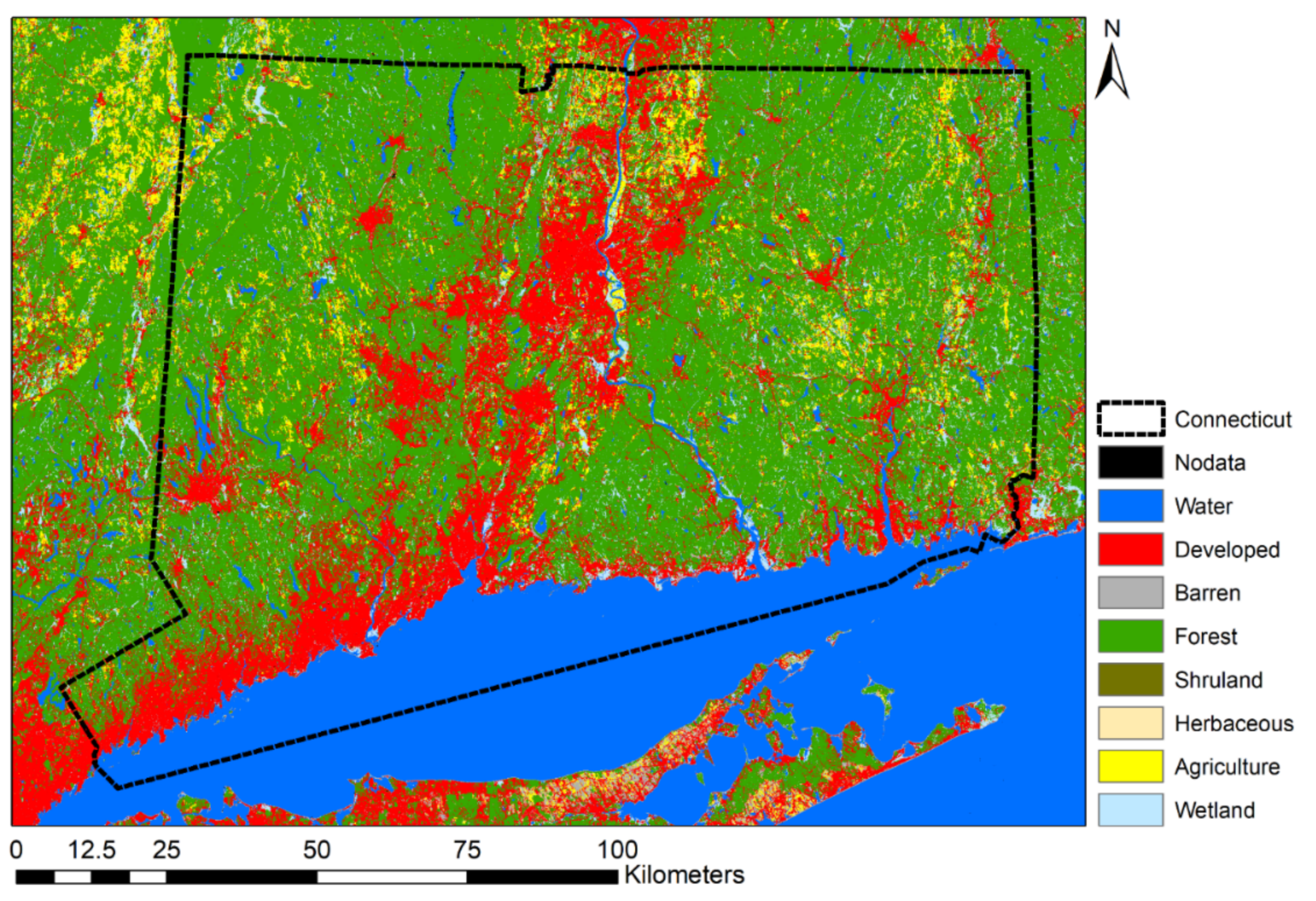
2.1. Study Area

We conducted this study in Connecticut, USA, which has a land area of 12,559 km2 and is predominantly covered by eastern broadleaf forest with Laurentian mixed forest in the northwestern part of the state [39]. The Köppen climate types included humid subtropical along Long Island Sound, to hot-summer humid continental and warm-summer humid continental moving upland.

2.2. Definitions of Vegetation Types

We identified three categories of vegetation based on ecological processes of succession, disturbance and regeneration, and hydrology, each of which contributes to the establishment or maintenance of young forest and shrubland vegetation (Table 1). We further used attributes of vegetation height and percent vegetation cover by height category, previous land cover type, and time since disturbance to define specific young forest and shrubland vegetation types. In this way, our definition of young forest and shrubland vegetation types contains greater detail than commonly used standards of forest vegetation types that primarily consider the percent of tree cover.
The succession category included vegetation types of reverting fields, old fields, and some shrublands that had previous land cover types of non-forest, and woody growth in shrub or tree form. Within this category, we distinguished the reverting field, shrubland, and transitional to forest vegetation types based on vegetation height and percent cover by height category (Table 2).
The forest disturbance and regeneration category included recently disturbed forest (partial or full canopy removal), regenerating clearcut, and regenerating forest (Table 1). Recently disturbed forest, regenerating clearcut, and regenerating forest all required a pre-disturbance land cover type of forest. We defined recently disturbed forest as disturbance 0 to 2 years prior, and regenerating forest as 3 to 20 years post-disturbance. Arrested reverting field and arrested shrubland originated from forest disturbance > 20 years yet remained in reverting field or shrubland vegetation height and structure, typically due to vegetation management activities. Further, we used vegetation height and percent cover by height category to distinguish regenerating clearcut from regenerating forest. Regenerating clearcut had up to 75% vegetation < 2.5 m tall, and <25% vegetation 2.5 m to 10 m tall, indicative of no residual trees to few residual trees in the stand. Regenerating forest had >25% vegetation 2.5 m to 10 m tall. Vegetation > 10 m was considered forest.
The hydrology category included select palustrine scrub-shrub and forested wetlands from a list provided by the Connecticut Department of Energy and Environmental Protection (Supplemental Table S1).

2.3. Segmentation, Pre-Classification, and Interpretation

2.3.1. Remotely Sensed Data

The multi-source and object-based approach to young forest and shrubland vegetation classification involved segmentation and pre-classification using information from multiple sensors, interpretation, and field verification (Figure 1). Remotely sensed data for segmentation and pre-classification included 3-band visible and 1-band infrared countywide 2018 National Agriculture Imagery Program (NAIP) mosaics for Connecticut collected using Leica ADS-100 digital sensor with a sampling distance of 0.40 m at 4983 m above mean terrain. We composited red, green, blue, and near-infrared (NIR) bands into a single 4-band image. We then resampled each band-image to 2-m resolution using bilinear resampling and clipped by county with a 500 m buffer prior to upload. It was necessary to reduce the file size for eventual import into Google Earth Engine [40] to comply with a size limit of max 10 GB file uploads.
We obtained vegetation height and structure information from LiDAR data from Connecticut Environmental Conditions Online (CT ECO) that were collected by the Leica ALS70 sensor with a point density of 2 pts/m2 on an airplane from 11 March 2016 through 16 April 2016 (http://www.cteco.uconn.edu/data/lidar/info_lidar.htm; last accessed on 20 May 2020). Based on the LiDAR data, CT ECO also provides the bare earth Digital Elevation Models (DEM) data with 1 m resolution. We processed the LiDAR 3D points for representing canopy heights of understory/forest by subtracting the bare earth DEM value from each LiDAR 3D point height. We clipped the ~3 m (10-foot) resolution canopy-height model (CHM) derived from 2016 statewide LiDAR returns by each county with a 500 m buffer prior to upload. We uploaded each countywide image and each countywide CHM to Google Earth Engine.
We obtained land cover, previous land cover type, and time since disturbance information from Landsat Analysis Ready Data (ARD) with cloud cover less than 80% from 1982 to 2019. The Landsat ARD include Landsats 4–5 Thematic Mapper (TM), Landsat 7 Enhanced Thematic Mapper Plus (ETM+), and Landsat 8 Operational Land Imager (OLI)/Thermal Infrared Sensor (TIRS) surface reflectance and brightness temperature products, which are provided with a data cube with a fixed spatial extent (5000 × 5000 30-m pixels) [41]. We used three Landsat ARD tiles for coverage of Connecticut with each tile consisting of more than 1600 Landsat images (Figure 2). This dataset also provided the cloud and cloud shadow mask generated by Fmask 3.3 [42]. We applied the Continuous Change Detection (CCD) and Continuous Classification (CC) [43] algorithm to the Landsat data and generated the annual land cover maps from 1985 to 2018. By comparing the 2018 land cover maps (30 m; Figure 3) to the maps of each year before 2018, we generated a previous land cover map (Figure 4) that indicated if a change occurred before 2018, and a time since the previous change map (Figure 5) that indicated how long ago the change occurred. We also generated the time-series model coefficient maps from CCDC algorithm, such as slopes of Red, NIR, and Shortwave Infrared (SWIR) bands that can be correlated with forest and shrubland growing conditions.

2.3.2. Preliminary Vegetation Classification

We used simple non-iterative clustering (SNIC; [44]) to classify clusters of similar pixels into superpixels based on similarity of spectral reflectance, spectral texture, vegetation height, and texture of vegetation height (Figure 1). In addition to the four spectral bands from NAIP (red, green, blue, NIR), we calculated Normalized Difference Vegetation Index (NDVI) and NDVI entropy and variance textures using a 25-pixel neighborhood. We also calculated vegetation height entropy and variance to include vegetation height in the SNIC. We used 60-pixel seed spacing for superpixels and exported ~1-m resolution results via Google Drive. We used ArcMap (ESRI 2019) to mosaic and then converted each county-level superpixel raster to a feature class and then merged polygons that were less than 100 m2 with the adjacent polygon with which it shared the longest border.
We resampled all data layers to match the original SNIC raster resolution for more consistent estimates of summarized data within superpixels. We generated superpixel-level zonal statistics data for each focal data layer and extracted results from rasterized outputs to points and spatially joined summaries to the segmented feature classes. At this point in the processing workflow, each superpixel contained a summary of data layers within its unique bounds. We then assigned preliminary vegetation and sub-vegetation types (Table 1) to each superpixel based on our ruleset (Table 2). Additionally, the sub-types of old field-reverting field, shrubland, reverting field to forest, shrubland to forest, and tall shrubland-young forest required a previous land cover type of non-forest. Conversely, recently disturbed forest, regenerating clearcut, and regenerating forest required a previous land cover type of forest and a disturbance more recent than 1998 (20 years old in 2018). Previously forest areas that were disturbed before 1998 and matched the vegetation height ruleset for old field-reverting field and shrubland were given a sub-type of arrested old field-reverting field and arrested shrubland, respectively. We identified the previous land cover type using the CCDC algorithm [43]. We then dissolved superpixels labeled with a vegetation type into preliminary, pre-interpretation complexes that contained one or more superpixels of one or more vegetation types. We calculated the area for each complex and selected those complexes over 1 ha in size for interpreter review. We used ArcMap for all processing.

2.3.3. Interpretation and Review

Interpreters reviewed all non-wetland superpixels within complexes of pre-labeled superpixels ≥1 ha using 2018 NAIP imagery at a viewing scale of 1:2000 to 1:3000 to remove errantly labeled superpixel (Figure 1). Interpreters confirmed the presence of shrub vegetation by looking for a textured appearance in the imagery. Superpixels pre-labeled as scrub-shrub and forested wetland were labeled according to their coincidence (>50%) with a subset of the National Wetland Inventory (NWI; [45]) and not reviewed in visual appearance or extent in this study. Interpreters removed pre-labeled superpixels that contained non-target vegetation (e.g., emergent wetland, plant nurseries, active orchards) or objects (e.g., solar panel arrays, cemetery headstones, livestock paddocks) that were confused with shrub vegetation in the CHM. Similarly, interpreters removed superpixels pre-labeled as a forest disturbance origin classification (i.e., regenerating clearcut, regenerating forest, recently disturbed forest) if they were associated with a land use conversion (e.g., forest cleared around structures and converted to manicured lawns).
If a pre-labeled superpixel contained a portion that was explicitly a non-target vegetation type, interpreters split the superpixel into two new superpixels and removed the remnant from classification. Interpreters split un-labeled superpixels directly adjacent to reviewed complexes of pre-labeled superpixels that contained a portion of the target vegetation and added the target portion to the classification.
Interpreters also added intact un-labeled superpixels to complexes of confirmed vegetation superpixels if they were adjacent and had a similar appearance to or presence of shrub height vegetation. These superpixels were assigned a vegetation classification label by the interpreter. This was done in areas where the CCDC algorithm underestimated the extent of forest disturbance and consequently disturbed superpixels were not pre-labeled.
Interpreters manually revised the classification label in rare instances if there was an obvious reason to do so. For example, if a large complex of superpixels pre-labeled as a forest disturbance origin class enveloped a superpixel pre-labeled with a non-disturbance origin classification (i.e., reverting field, shrubland, transitional to forest), the non-disturbance superpixels were switched to the adjacent superpixel’s classification. This was done due to the CCDC algorithm either under-representing the disturbed area or misclassifying the pre-disturbance land cover as non-forest.
Upon completion of the interpretation and review phase, interpreters assembled new vegetation complexes by dissolving superpixels confirmed as target vegetation types, including superpixels labeled as palustrine scrub-shrub and forested wetland. Thus, vegetation complexes reported include one or more superpixels of one or more vegetation types reviewed by interpreters.

2.4. Field Verification and Accuracy Assessment of Vegetation Classification

2.4.1. Sample Design, Sample Size, and Allocation to Strata

We estimated area and assessed accuracy of young forest and shrubland vegetation types following good practices detailed in Olofsson et al. [46]. We used a two-stage, stratified cluster sampling approach to collect verification data for each vegetation type [47,48]. The first stage consisted of a geographically stratified (by county) random sample of vegetation complexes selected from a population of complexes located on protected areas with public access. The population of vegetation complexes was restricted to protected areas with at least 1 complex ≥1 ha in size and 2 or more vegetation types within a protected area, such that we could gain efficiency by verifying at least two vegetation types within each protected area. The second stage consisted of a stratified random sample of vegetation superpixels by vegetation type within selected protected areas. Only superpixels larger than 400 m2 were eligible for selection. In instances of > 1 superpixel per vegetation type per complex, we randomly selected up to three superpixels to sample for each vegetation type, to increase efficiency further. Although the sample design used probabilistic sampling, we acknowledge that restricting verification to publicly accessible areas of the mapped region assumed that accuracy estimates were representative of the entire mapped region [49,50].
The sample size (n) was determined with a target standard error for overall accuracy (S(O)) of 0.01, from the mapped area proportion (Wi) of nine vegetation types within Connecticut, standard deviation of each stratum (Si), and conjectured user’s accuracy (Ui) [46,51]. We assigned approximate values of user’s accuracy (Ui) of 0.903 for forest and 0.728 for non-forest types ([52], Table 3: Level I Forest and average of Level 1 Non-forest, respectively), 0.850 for recently disturbed forest, regenerating clearcut, and regenerating forest ([43], Table 5 therein: lowest user accuracy of deciduous forest, coniferous forest, and mixed forest), and 0.817 for reverting field, shrubland, and transitional to forest types ([52], Table 2 therein: Level II Shrubland). The resulting sample size was n = 1287 samples (Supplemental Table S2), which, if allocated proportionately, would grossly underrepresent reverting field, shrubland, young forest, and regenerating forest types and subsequently lead to large standard error for estimated user’s accuracy [46]. Therefore, we allocated 100 samples to each of the rare types, and proportionately allocated remaining samples to the forest and non-forest types (Supplemental Table S2). Each of the samples was distributed by geographic region (county) per the first stage, and subsequently by vegetation type in the second stage (Supplemental Table S2).

2.4.2. Response Design with Field and Digital Reference Data

We used a geographic information system (GIS) to randomly select up to three superpixels of each shrubland vegetation type present within a protected area [53]. We visited each randomly selected superpixel, recorded the vegetation height, visually assessed the superpixel, and assigned a vegetation type based on the vegetation height and visual assessment (Figure 1). We used aerial imagery (NAIP, years 2004 to 2018) to verify young forest types since a pre-disturbance land cover classification of forest could not reliably be ascertained in the field. For the forest and non-forest background types, we randomly selected single pixels (30-m) from the CCDC derived land cover in 2018, and used aerial imagery (NAIP, 2018) to verify the land cover classification. Pixels classified as wetland were excluded from the population as the land cover classification map did not distinguish forested wetlands from non-forested wetlands.

2.4.3. Accuracy Assessment Analysis

We used an error matrix to cross-tabulate the classified vegetation against the reference data, which enabled accuracy assessment and area estimation with confidence intervals [46]. In the cross-tabulation table, the rows constitute the classified vegetation (i), the columns the reference vegetation (j), and the cell value Pij indicates the proportion of area in the full region of interest that has map type i and reference type j. Here, the region of interest is the state-wide map of young forest and shrubland vegetation types. We report the error matrix, the proportion of each type as determined from the map, estimated user’s accuracy, producer’s accuracy, and overall accuracy using the estimated area proportions, and the area of each vegetation type with confidence intervals.

3. Results

3.1. Young Forest and Shrubland Vegetation

3.1.1. Statewide

The segmentation, classification, and interpretation procedure resulted in 5,121,477 superpixels statewide, of which interpreters reviewed 165,067 pre-classified superpixels that occurred in vegetation complexes ≥1 ha in size (Supplemental Table S3). Interpreters did not review 36,235 superpixels that were pre-classified as palustrine scrub-shrub and forested wetland as they had >50% spatial overlap with NWI polygons.
Interpreters reviewed 123,323 superpixels totaling 34,147 ha of reverting field, shrubland, transitional to forest, recently disturbed forest, regenerating clearcut, regenerating forest, and palustrine scrub-shrub and forested wetlands in Connecticut (Supplemental Table S4). Of those superpixels, 73,055 occurred in vegetation complexes ≥2 ha in size and totaled 20,953 ha (Supplemental Table S4).

3.1.2. Accuracy Assessment

The accuracy assessment of the young forest and shrubland vegetation map was conducted using 1283 verification samples, of which 252 were field visits to reverting field, shrubland, and transitional to forest vegetation types, and 1031 were aerial photo interpretations of forest disturbance and regeneration vegetation types and the background forest and non-forest types (Table 3). Classification accuracy was calculated from the estimated area proportions of each type (Supplemental Table S5).
The young forest and shrubland vegetation map had overall accuracy of 88.2 ± 2.3% (95% confidence interval). Producer’s accuracy, the proportion of a land cover type on the ground being classified as such, was very high for recently disturbed forest (95.4 ± 8.6%) and moderate for transitional to forest (55.0 ± 21.3%) and reverting field (50.3 ± 41.4%) (Table 4). User’s accuracy, the proportion of a mapped vegetation type that is actually that type, was high for transitional to forest (84.0 ± 7.0%) and ranged from 62.3 to 66.7% for the other young forest and shrubland vegetation types (Table 4). The estimated area (95% CI) was highest for transitional to forest (18,656 ± 7256 ha), followed by regenerating forest (12,424 ± 8050 ha) and regenerating clearcut (5005 ± 5078 ha). Recently disturbed forest (986 ± 154 ha) and shrubland (1464 ± 552 ha) had the lowest estimated area statewide (Table 4).
Of the 1283 reference samples used in the accuracy assessment, 272 were mapped as the wrong type (Table 3). Careful inspection of the error matrix revealed that the primary source of classification error was the confusion of mapped vegetation types for actual (reference, on the ground) non-forest, which occurred 16 times for reverting field and totaled 97 of the 272 classification errors across the young forest and shrubland vegetation types. The next most frequent source of classification error was the confusion of an actual young forest or shrubland vegetation type for a different young forest and shrubland vegetation type. For example, shrubland was mapped as reverting field five times, transitional to forest five times, and regenerating clearcut nine times, yet was never mapped as forest or non-forest.

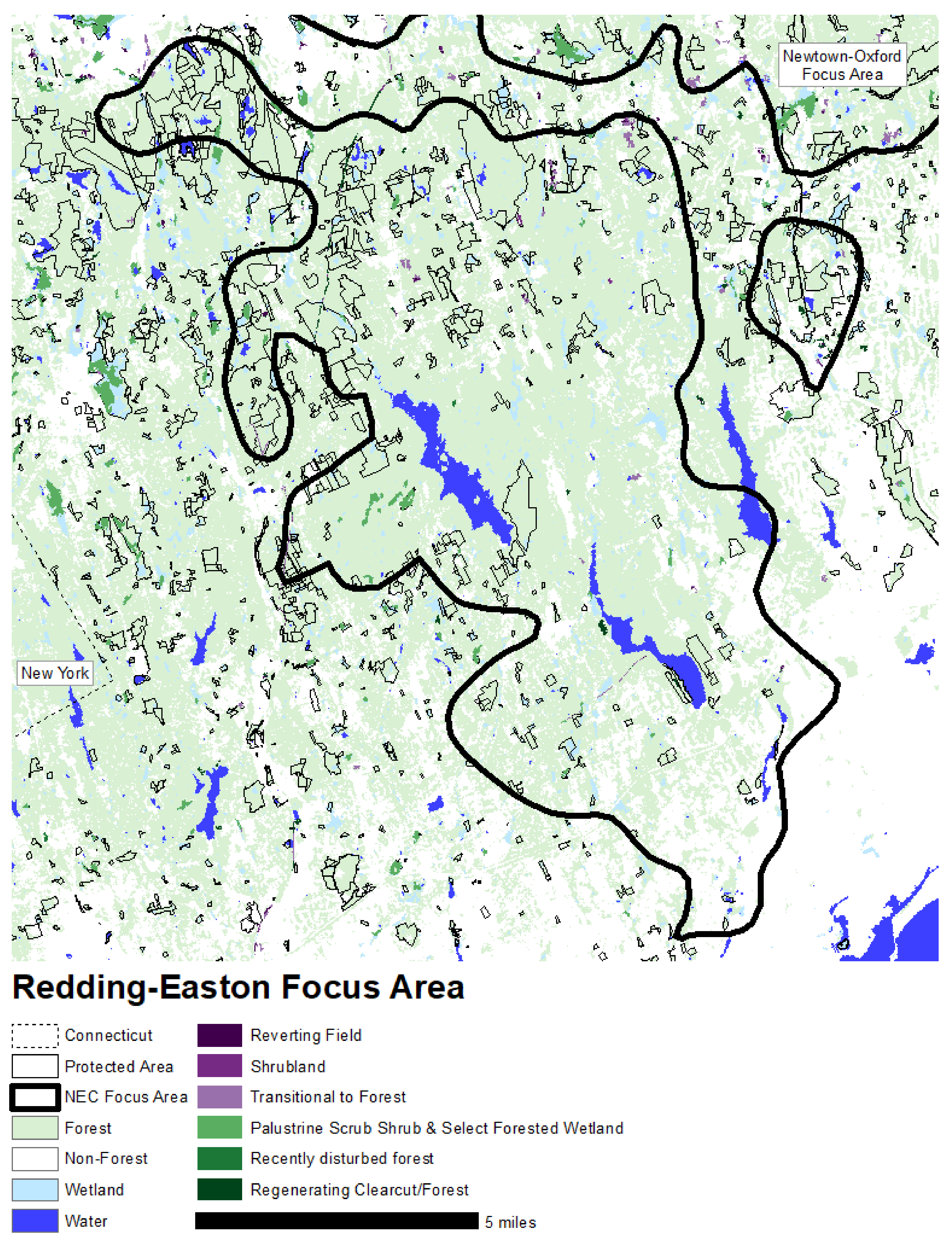
3.2. New England Cottontail Focus Areas

The segmentation, classification, and interpretation procedure identified 7827 ha of young forest and shrubland vegetation in vegetation complexes ≥2 ha in size within New England cottontail Focus Areas (Table 5). Goshen Uplands Focus Area had 1499 ha of young forest and shrubland vegetation (Figure 6), the most of all Focus Areas, while Redding-Easton had the least at 178 ha (Figure 7). Across all Focus Areas, the predominant vegetation type by area was transitional to forest with 2388 ha, followed by palustrine scrub-shrub and forested wetlands with 2344 ha (Table 5).
When summarized by vegetation complex size, where a complex consists of 1 or more adjacent young forest and shrubland vegetation types, the majority of the area was in complexes 4 to 10 ha in size (2835 ha), followed by complexes 2 to 4 ha in size (2434 ha) (Table 6). Notably, 1242 ha of young forest and shrubland vegetation exists in complexes exceeding 20 ha in size, although 455 ha were palustrine scrub-shrub and forested wetland (Table 6). Separate tables (Supplemental Tables S6–S17) and figures (Supplemental Figures S1–S12) are provided for each New England cottontail Focus Area.
Summaries of the young forest and shrubland vegetation by ownership for New England Cottontail Focus Areas revealed that 1864 ha are in some form of protected ownership, comprised of 1136 ha of state lands, 427 ha of other lands, 204 ha of local lands, 93 ha of private lands, and 2 ha of federal lands (Table 7). The percentage of young forest and shrubland vegetation types in protected status ranged from 12.2% in the Scotland-Canterbury Focus Area to 34.9% in the Redding-Easton Focus Area and totaled 23.8% across all focus areas.

3.3. American Woodcock Focus Area

When summarized by American woodcock Focus Area, the segmentation, classification, and interpretation procedure identified 11,644 ha of young forest and shrubland vegetation that occurs in vegetation complexes ≥2 ha in size (Table 8). The predominant vegetation type by area was palustrine scrub-shrub and forested wetlands with 3389 ha, followed by transitional to forest with 3325 ha (Table 8).

4. Discussion

The goals of this project were to map and provide area estimates for young forest and shrubland vegetation types in a temperate forest, and to summarize area within the New England Cottontail Focus Areas, the American Woodcock Focus Area, and throughout the state for all patches ≥2 ha in size. The multi-source, object-based, and hand digitizing approaches provided an area-adjusted estimate of 42,944 ha of young forest and shrubland vegetation in Connecticut with overall map accuracy of 88.2% (95% CI 2.3%; Table 4). A total of 20,953 ha of young forest and shrubland vegetation occurred in complexes ≥2 ha in size (Supplemental Table S4), of which 7827 ha occurred within New England Cottontail Focus Areas (Table 5) and 11,644 ha occurred within the American Woodcock Focus Area (Table 8).
Young forest and shrubland vegetation constituted 3.3% of Connecticut’s total land cover and 6.3% of forest cover as of 2018. Previous studies estimated the seedling-sapling stage at 2.8% of Connecticut’s total land cover and 5% of forest cover in 1998 [54], and 4.1% of Connecticut’s total land cover and 5.6% of forest cover in 2011 [55]. Although the 2019 estimates are consistent with those of the past 20 years, concerted efforts are needed to restore, maintain, or manage young forest and shrubland vegetation in Connecticut. These vegetation types originate from disturbance and succession processes, which since the year 1500 in the New England region consisted largely of fires from anthropogenic sources punctuated by catastrophic winds from hurricanes and episodic flooding by beavers [23,56,57,58]. Human fires created and maintained open grassland and savannas, typically near coastal areas and rivers, though fires were used to drive game on upland sites as well [59,60]. Hurricanes produced a different pattern of young forest and shrubland vegetation that, in the case of the 1938 hurricane, extended up to 100 km inland affecting primarily south- and east-facing slopes and the northwestern shore of lakes [59]. Anthropogenic agents remain the predominant disturbance processes today [61], though Lymantria dispar outbreaks and emerald ash borer (Agrilus planipennis) have caused widespread mortality events in recent years and may result in more young forest and shrubland vegetation.
The predominance of palustrine scrub-shrub and forested wetland vegetation warrants a closer look at both their spatial extent and the accuracy of the National Wetlands Inventory map from which they were derived. Of the 34,147 ha of young forest, shrubland, and palustrine scrub-shrub and forested wetland vegetation statewide, the latter constituted 27.6% of the area statewide (Supplemental Table S4). Seasonal and annual variations in hydrology, such as high precipitation years that increase surface water extent and water depth, drive plant mortality and conversely drought facilitates establishment of shrubs and trees in palustrine systems [62,63]. Subsequently, the success of remote-sensing approaches to palustrine wetland mapping rests on high spatial resolution data available over time and accurate classification approaches that take advantage of spectral, textural, geophysical, and geomorphological characteristics of wetlands [64,65,66,67]. Similar to the issues raised with mapping wetlands, the accuracies of young forest and shrubland classes were relatively low. We attribute the low accuracy to several factors, including that young forest and shrubland vegetation types are ephemeral, have small areal extent (~40% of segments <2 ha in size; Supplemental Table S4), and have structural differences separated by <2.5 m (e.g., vegetation height). Future studies will benefit from higher resolution imagery and LiDAR data that are inevitable.
This project mapped vegetation types that are considered habitats for young forest- and shrubland-dependent wildlife species. In doing so, we defined vegetation types based on disturbance and succession processes and hydrology, as well as vegetation height, percent cover by height category, previous land cover type, and time since disturbance. While valuable in and of itself, we are excited about its application in future studies of biodiversity conservation. In this application, the biology of the species, including patch size, distance between patches, interspersion of vegetation types, and the matrix vegetation all need to be considered. For example, recent studies on New England cottontail suggest a minimum patch size of 7 ha, provide evidence of limited dispersal ability, and find higher survival in regenerating forest stands with high residual canopy cover than in stands with low residual canopy cover [68,69,70]. Of the 7827 ha of young forest and shrubland vegetation ≥2 ha in size within New England Cottontail Focus Areas, 2835 ha were in complexes 4 to 10 ha in size, and only 2558 ha were in complexes exceeding 20 ha in size (Table 6). American woodcock habitat requirements vary by season and include open habitats used for display and young to mid-age forests used for feeding, roosting, and nesting during the breeding season [71]. The size of openings and interspersion of young forests, wetlands, and reverting fields are important habitat features for woodcock [72,73]. Imposing interspersion or adjacency requirements within an area approximating the average home range size (15 ha, range 0.3–17 ha) for male woodcock [74] to the young forest and shrubland vegetation map is recommended. Once these additional species-specific factors are considered, there may be substantially less area of young forest, shrubland, and palustrine scrub-shrub wetlands that would be habitat for New England cottontail and American Woodcock.
The young forest and shrubland habitat vegetation map may also be used to guide the location of young forest and shrubland conservation and management efforts. For example, the extent of New England cottontail Focus Areas was based on New England cottontail occupancy (current or historical) and with consideration for existing habitat and potential to implement management for new habitat [37,38]. Retention of existing Focus Areas is supported as all contain young forest and shrubland vegetation (Table 5). Additionally, the statewide map of young forest and shrubland vegetation provides an opportunity to adjust boundaries of existing focus areas, as well as to develop new focus areas where concentrations of young forest and shrubland vegetation exist. The young forest and vegetation map may also be used to improve biodiversity surveys. An overlay of survey effort and New England cottontail detections on the young forest and shrubland vegetation map would be a simple first step towards understanding and reducing sampling bias, that is, the distribution of sampling effort with respect to vegetation types and ownerships within and outside of existing focus areas. Ideally, the statewide young forest and shrubland vegetation map would guide surveys for New England cottontail and other species dependent on these habitats, to potentially identify unknown populations.

5. Conclusions

The multi-source, object-based approach that we developed to map young forest and shrubland vegetation in a temperate forest utilized strengths of remote sensing (large spatial extent with good temporal coverage), LiDAR (vegetation height and vertical structure), and aerial imagery (high resolution), and achieved high accuracy overall. The resulting map distinguishes stages of succession and informs decision-making for forest management and wildlife conservation. Although our estimates are consistent with those of the past 20 years, concerted efforts are needed to restore, maintain, or manage young forest and shrubland vegetation in Connecticut.

Supplementary Materials

The following supporting information can be downloaded at: https://www.mdpi.com/article/10.3390/rs14051091/s1, Figure S1: Young forest and shrubland vegetation map for the Goshen Upland Focus Area; Figure S2: Young forest and shrubland vegetation map for the Lebanon Focus Area; Figure S3: Young forest and shrubland vegetation map for the Ledyard-Coast Focus Area; Figure S4: Young forest and shrubland vegetation map for the Lower Connecticut River Focus Area; Figure S5: Young forest and shrubland vegetation map for the Lower Housatonic River Focus Area; Figure S6: Young forest and shrubland vegetation map for the Middle Housatonic River Focus Area; Figure S7: Young forest and shrubland vegetation map for the Newtown-Oxford Focus Area; Figure S8: Young forest and shrubland vegetation map for the Northern Border Focus Area; Figure S9: Young forest and shrubland vegetation map for the Pachaug Focus Area; Figure S10: Young forest and shrubland vegetation map for the Redding-Easton Focus Area; Figure S11: Young forest and shrubland vegetation map for the Scotland-Canterbury Focus Area; Figure S12: Young forest and shrubland vegetation map for the Upper Housatonic River Focus Area; Table S1: Palustrine Scrub-Shrub and Forested Wetlands types in Connecticut. Area (in ha) provided from National Wetland Inventory shapefile. List derived by Lisa Wahle from the National Wetlands Inventory. The Wetlands Code Interpreter provides descriptions for each type. P = Palustrine; FO1 = Forested, broad-leaved deciduous; SS1 = Scrub-Shrub, broad-leaved deciduous; SS3 = Scrub-shrub, broad-leaved evergreen; EM1 = Emergent, subclass persistent; A = Temporary flooded; B = Seasonally saturated; E = Seasonally flooded/saturated; a = Acid water chemistry; b = Beaver modified; d = Partially drained/ditched; h = Diked/impounded; x = Excavated; Table S2: Allocation of sample size to strata based on mapped area proportion (Wi), conjectured user’s accuracy (Ui), and standard deviation (Si) of the strata. Area in hectares; Table S3: Summary of number of segments, reviewed segments, and segments with vegetation check by county. Only segments within vegetation complexes ≥1 ha were reviewed; Table S4: Statewide summary of confirmed vegetation segments by classification and complex size; Table S5: Error matrix populated by estimated proportion of area within Connecticut; Table S6: Hectares of young forest and shrubland vegetation types by complex size for the Goshen Uplands Focus Area; Table S7: Hectares of young forest and shrubland vegetation types by complex size for the Lebanon Focus Area; Table S8: Hectares of young forest and shrubland vegetation types by complex size for the Ledyard-Coast Focus Area; Table S9: Hectares of young forest and shrubland vegetation types by complex size for the Lower Connecticut River Focus Area; Table S10: Hectares of young forest and shrubland vegetation types by complex size for the Lower Housatonic River Focus Area; Table S11: Hectares of young forest and shrubland vegetation types by complex size for the Middle Housatonic Focus Area; Table S12: Hectares of young forest and shrubland vegetation types by complex size for the Newtown-Oxford Focus Area; Table S13: Hectares of young forest and shrubland vegetation types by complex size for the Northern Border Focus Area; Table S14: Hectares of young forest and shrubland vegetation types by complex size for the Pachaug Focus Area; Table S15: Hectares of young forest and shrubland vegetation types by complex size for the Redding-Easton Focus Area; Table S16: Hectares of young forest and shrubland vegetation types by complex size for the Scotland-Canterbury Focus Area; Table S17: Hectares of young forest and shrubland vegetation types by complex size for the Upper Housatonic Focus Area.

Author Contributions

Conceptualization, C.D.R. and Z.Z.; methodology, Z.Z., N.M. and S.Q.; formal analysis, E.H.B., N.M., D.R. and S.Q.; writing—original draft preparation, C.D.R., N.M., D.R. and S.Q.; writing—review and editing, C.D.R., E.H.B., N.M., D.R., S.Q. and Z.Z.; supervision, C.D.R. and Z.Z.; funding acquisition, C.D.R. and Z.Z. All authors have read and agreed to the published version of the manuscript.

Funding

This project was funded by a grant from the Connecticut Department of Energy and Environmental Protection, Wildlife Division.

Data Availability Statement

The young forest and shrubland vegetation map is hosted on CT ECO (https://cteco.uconn.edu/ accessed on 16 December 2021).

Acknowledgments

We thank L. Wahle, J. Wilson, H. Kilpatrick, and T. Steeves of the Connecticut Department of Energy and Environmental Protection, Wildlife Division, for discussions on young forest and shrubland vegetation and reviewing the final report from which this paper was developed.

Conflicts of Interest

The authors declare no conflict of interest. The funders had no role in the design of the study; in the collection, analyses, or interpretation of data; in the writing of the manuscript, or in the decision to publish the results.

References

  1. Food and Agricultural Organization of the United Nations. Global Forest Resources Assessment 2020; Main Report; Food and Agricultural Organization of the United Nations: Rome, Italy, 2020. [Google Scholar] [CrossRef]
  2. Brockerhoff, E.G.; Barbaro, L.; Castagneyrol, B.; Forrester, D.I.; Gardiner, B.; González-Olabarria, J.R.; Lyver, P.O.; Meurisse, N.; Oxbrough, A.; Taki, H.; et al. Forest biodiversity, ecosystem functioning and the provision of ecosystem services. Biodivers. Conserv. 2017, 26, 3005–3035. [Google Scholar] [CrossRef] [Green Version]
  3. Ellison, D.; Morris, C.E.; Locatelli, B.; Sheil, D.; Cohen, J.; Murdiyarso, D.; Gutierrez, V.; van Noordwijk, M.; Creed, I.F.; Pokorny, J.; et al. Trees, forests and water: Cool insights for a hot world. Glob. Environ. Chang. 2017, 43, 51–61. [Google Scholar] [CrossRef]
  4. Goeking, S.A.; Tarboton, D.G. Forests and Water Yield: A Synthesis of Disturbance Effects on Streamflow and Snowpack in Western Coniferous Forests. J. For. 2020, 118, 172–192. [Google Scholar] [CrossRef] [Green Version]
  5. Dixon, R.K.; Solomon, A.M.; Brown, S.; Houghton, R.A.; Trexier, M.C.; Wisniewski, J. Carbon Pools and Flux of Global Forest Ecosystems. Science 1994, 263, 185–190. [Google Scholar] [CrossRef] [PubMed]
  6. Wunder, S.; Angelsen, A.; Belcher, B. Forests, Livelihoods, and Conservation: Broadening the Empirical Base. World Dev. 2014, 64, S1–S11. [Google Scholar] [CrossRef] [Green Version]
  7. Karjalainen, E.; Sarjala, T.; Raitio, H. Promoting human health through forests: Overview and major challenges. Environ. Health Prev. Med. 2009, 15, 1. [Google Scholar] [CrossRef]
  8. Hall, F.G.; Botkin, D.B.; Strebel, D.E.; Woods, K.D.; Goetz, S.J. Large-Scale Patterns of Forest Succession as Determined by Remote Sensing. Ecology 1991, 72, 628–640. [Google Scholar] [CrossRef]
  9. Masek, J.G.; Huang, C.; Wolfe, R.; Cohen, W.; Hall, F.; Kutler, J.; Nelson, P. North American forest disturbance mapped from a decadal Landsat record. Remote Sens. Environ. 2008, 112, 2914–2926. [Google Scholar] [CrossRef]
  10. Hansen, M.; Stehman, S.V.; Potapov, P.V.; Loveland, T.R.; Townshend, J.R.G.; DeFries, R.S.; Pittman, K.W.; Arunarwati, B.; Stolle, F.; Steininger, M.K.; et al. Humid tropical forest clearing from 2000 to 2005 quantified using multi-temporal and multi-resolution remotely sensed data. Proc. Natl. Acad. Sci. USA 2008, 105, 9439–9444. [Google Scholar] [CrossRef] [Green Version]
  11. DeFries, R.S.; Houghton, R.A.; Hansen, M.C.; Field, C.B.; Skole, D.; Townshend, J. Carbon emissions from tropical land use change based on satellite observations for the 1980s and 90s. Proc. Natl. Acad. Sci. USA 2002, 99, 14256–14261. [Google Scholar] [CrossRef] [Green Version]
  12. Hansen, M.C.; Stehman, S.V.; Potapov, P.V. Quantification of global gross forest cover loss. Proc. Natl. Acad. Sci. USA 2010, 107, 8650–8655. [Google Scholar] [CrossRef] [PubMed] [Green Version]
  13. Achard, F.; Eva, H.D.; Glinni, A.; Mayaux, P.; Richards, T.; Stibig, H.-J. Identification of Deforestation Hot Spot Areas in the Humid Tropics; EUR 18079 EN; European Commission: Luxembourg, 1998. [Google Scholar]
  14. Harris, G.M.; Pimm, S.L. Bird species’ tolerance of secondary forest habitats and its effects on extinction. Conserv. Biol. 2004, 18, 1607–1616. [Google Scholar]
  15. Prishchepov, A.; Radeloff, V.C.; Baumann, M.; Kuemmerle, T.; Müller, D. Effects of institutional changes on land use: Agricultural land abandonment during the transition from state-command to market-driven economies in post-Soviet Eastern Europe. Environ. Res. Lett. 2012, 7, 024021. [Google Scholar] [CrossRef]
  16. Davis, K.F.; Koo, H.I.; Dell’Angelo, J.; D’Odorico, P.; Estes, L.; Kehoe, L.J.; Kharratzadeh, M.; Kuemmerle, T.; Machava, D.; De Jesus Rodrigues Pais, A.; et al. Tropical forest loss enhanced by large-scale land acquisitions. Nat. Geosci. 2020, 13, 482–488. [Google Scholar] [CrossRef]
  17. Mackey, B.; DellaSala, D.A.; Kormos, C.; Lindenmayer, D.; Kumpel, N.; Zimmerman, B.; Hugh, S.; Young, V.; Foley, S.; Arsenis, K.; et al. Policy options for the world’s primary forests in multilateral environmental agreements. Conserv. Lett. 2015, 8, 139–147. [Google Scholar] [CrossRef] [Green Version]
  18. Drake, J.B.; Dubayah, R.O.; Clark, D.B.; Knox, R.G.; Blair, J.; Hofton, M.A.; Chazdon, R.; Weishampel, J.F.; Prince, S. Estimation of tropical forest structural characteristics using large-footprint lidar. Remote Sens. Environ. 2002, 79, 305–319. [Google Scholar] [CrossRef]
  19. Harmon, M.E.; Ferrell, W.K.; Franklin, J.F. Effects on Carbon Storage of Conversion of Old-Growth Forests to Young Forests. Science 1990, 247, 699–702. [Google Scholar] [CrossRef] [Green Version]
  20. Foody, G.M.; Palubinskas, G.; Lucas, R.M.; Curran, P.J.; Honzak, M. Identifying terrestrial carbon sinks: Classification of successional stages in regenerating tropical forest from Landsat TM data. Remote Sens. Environ. 1996, 55, 205–216. [Google Scholar] [CrossRef]
  21. Kuemmerle, T.; Olofsson, P.; Chaskovskyy, O.; Baumann, M.; Ostapowicz, K.; Woodcock, C.E.; Houghton, R.A.; Hostert, P.; Keeton, W.S.; Radeloff, V.C. Post-Soviet farmland abandonment, forest recovery, and carbon sequestration in western Ukraine. Glob. Chang. Biol. 2010, 17, 1335–1349. [Google Scholar] [CrossRef]
  22. Bormann, F.H.; Likens, G.E. Pattern and Process in a Forested Ecosystem; Springer: New York, NY, USA, 1979. [Google Scholar]
  23. Foster, D.R.; Motzkin, G.; Slater, B. Land-Use History as Long-Term Broad-Scale Disturbance: Regional Forest Dynamics in Central New England. Ecosystems 1998, 1, 96–119. [Google Scholar] [CrossRef]
  24. Aber, J.; Christensen, N.L.; Fernandez, I.; Franklin, J.F.; Hidinger, L.; Hunter, J.; MacMahon, J.A.; Mladenoff, D.; Pastor, J.; Perry, D.A.; et al. Applying ecological principles to management of the US national forests. Ecology 2000, 6, 20. [Google Scholar]
  25. Franklin, J.F.; Spies, T.A.; Van Pelt, R.; Carey, A.B.; Thornburgh, D.A.; Berg, D.R.; Lindenmayer, D.B.; Harmon, M.E.; Keeton, W.S.; Shaw, D.C.; et al. Disturbances and structural development of natural forest ecosystems with silvicultural implications, using Douglas-fir forests as an example. For. Ecol. Manag. 2002, 155, 399–423. [Google Scholar] [CrossRef]
  26. DeGraaf, R.M.; Yamasaki, M. Options for managing early-successional forest and shrubland bird habitats in the northeastern United States. For. Ecol. Manag. 2003, 185, 179–191. [Google Scholar] [CrossRef]
  27. Gibson, L.; Lee, T.M.; Koh, L.P.; Brook, B.; Gardner, T.A.; Barlow, J.; Peres, C.; Bradshaw, C.; Laurance, W.F.; Lovejoy, T.E.; et al. Primary forests are irreplaceable for sustaining tropical biodiversity. Nature 2011, 478, 378–381. [Google Scholar] [CrossRef]
  28. Nikodemus, O.; Bell, S.; Grīne, I.; Liepiņš, I. The impact of economic, social and political factors on the landscape structure of the Vidzeme Uplands in Latvia. Landsc. Urban Plan. 2005, 70, 57–67. [Google Scholar] [CrossRef]
  29. Müller, D.; Munroe, D. Changing Rural Landscapes in Albania: Cropland Abandonment and Forest Clearing in the Postsocialist Transition. Ann. Assoc. Am. Geogr. 2008, 98, 855–876. [Google Scholar] [CrossRef]
  30. Kuemmerle, T.; Hostert, P.; Radeloff, V.C.; van der Linden, S.; Perzanowski, K.; Kruhlov, I. Cross-border comparison of post-socialist farmland abandonment in the Carpathians. Ecosystems 2008, 11, 614–628. [Google Scholar] [CrossRef]
  31. Baumann, M.; Kuemmerle, T.; Elbakidze, M.; Ozdogan, M.; Radeloff, V.C.; Keuler, N.S.; Prishchepov, A.V.; Kruhlov, I.; Hostert, P. Patterns and drivers of post-socialist farmland abandonment in Western Ukraine. Land Use Policy 2011, 28, 552–562. [Google Scholar] [CrossRef]
  32. Loboda, T.V.; Chen, D. Spatial distribution of young forests and carbon fluxes within recent disturbances in Russia. Glob. Chang. Biol. 2016, 23, 138–153. [Google Scholar] [CrossRef]
  33. Naidoo, L.; Mathieu, R.; Main, R.; Wessels, K.; Asner, G.P. L-band Synthetic Aperture Radar imagery performs better than optical datasets at retrieving woody fractional cover in deciduous, dry savannahs. Int. J. Appl. Earth Obs. Geoinf. 2016, 52, 54–64. [Google Scholar] [CrossRef]
  34. Carreiras, J.M.B.; Jones, J.; Lucas, R.M.; Shimabukuro, Y.E. Mapping major land cover types and retrieving the age of secondary forests in the Brazilian Amazon by combining single-date optical and radar remote sensing data. Remote Sens. Environ. 2017, 194, 16–32. [Google Scholar] [CrossRef] [Green Version]
  35. Baumann, M.; Levers, C.; Macchi, L.; Bluhm, H.; Waske, B.; Gasparri, N.I.; Kuemmerle, T. Mapping continuous fields of tree and shrub cover across the Gran Chaco using Landsat 8 and Sentinel-1 data. Remote Sens. Environ. 2018, 216, 201–211. [Google Scholar] [CrossRef]
  36. Bispo, P.D.C.; Pardini, M.; Papathanassiou, K.P.; Kugler, F.; Balzter, H.; Rains, D.; Santos, J.R.d.; Rizaev, I.G.; Tansey, K.; de Santos, M.N.; et al. Mapping forest successional stages in the Brazilian Amazon using forest heights derived from TanDEM-X SAR interferometry. Remote Sens. Environ. 2019, 232, 111194. [Google Scholar] [CrossRef]
  37. Fuller, S. Conservation Strategy for the New England Cottontail (Sylvilagus transitionalis). 2012. Available online: https://newenglandcottontail.org/sites/default/files/research_documents/conservation_strategy_final_12-3-12.pdf (accessed on 16 December 2021).
  38. Fuller, S.; Tur, A. Conservation Strategy for the New England Cottontail (Sylvilagus transitionalis), Updated. 2017. Available online: https://newenglandcottontail.org/sites/default/files/research_documents/Conservation%20Strategy%20Updated%20%203-16-17.pdf (accessed on 16 December 2021).
  39. Bailey, R.G. Ecoregions: The Ecosystem Geography of the Oceans and Continents, 2nd ed.; Springer: New York, NY, USA, 2014; 192p. [Google Scholar]
  40. Gorelick, N.; Hancher, M.; Dixon, M.; Ilyushchenko, S.; Thau, D.; Moore, R. Google Earth Engine: Planetary-scale geospatial analysis for everyone. Remote Sens. Environ. 2017, 202, 18–27. [Google Scholar] [CrossRef]
  41. Dwyer, J.; Roy, D.; Sauer, B.; Jenkerson, C.; Zhang, H.; Lymburner, L. Analysis Ready Data: Enabling Analysis of the Landsat Archive. Remote Sens. 2018, 10, 1363. [Google Scholar] [CrossRef]
  42. Zhu, Z.; Wang, S.; Woodcock, C.E. Improvement and expansion of the Fmask algorithm: Cloud, cloud shadow, and snow detection for Landsats 4–7, 8, and Sentinel 2 images. Remote Sens. Environ. 2015, 159, 269–277. [Google Scholar] [CrossRef]
  43. Zhu, Z.; Woodcock, C.E. Continuous change detection and classification of land cover using all available Landsat data. Remote Sens. Environ. 2014, 144, 152–171. [Google Scholar] [CrossRef] [Green Version]
  44. Achanta, R.; Süsstrunk, S. Superpixels and Polygons Using Simple Non-iterative Clustering. In Proceedings of the 2017 IEEE Conference on Computer Vision and Pattern Recognition (CVPR), Honolulu, HI, USA, 21–26 July 2017; pp. 4895–4904. [Google Scholar]
  45. U.S. Fish and Wildlife Service. National Wetlands Inventory Website; U.S. Department of the Interior, Fish and Wildlife Service: Washington, DC, USA, 2021. Available online: http://www.fws.gov.wetlands (accessed on 9 September 2021).
  46. Olofsson, P.; Foody, G.M.; Herold, M.; Stehman, S.V.; Woodcock, C.E.; Wulder, M.A. Good practices for estimating area and assessing accuracy of land change. Remote Sens. Environ. 2014, 148, 42–57. [Google Scholar] [CrossRef]
  47. Stehman, S.V.; Sohl, T.L.; Loveland, T.R. Statistical sampling to characterize recent United States land-cover change. Remote Sens. Environ. 2003, 86, 517–529. [Google Scholar] [CrossRef]
  48. Stehman, S.V.; Wickham, J.D.; Wade, T.G.; Smith, J.H. Designing a Multi-Objective, Multi-Support Accuracy Assessment of the 2001 National Land Cover Data (NLCD 2001) of the Conterminous United States. Photogramm. Eng. Remote Sens. 2008, 74, 1561–1571. [Google Scholar] [CrossRef]
  49. Stehman, S.V. Statistical rigor and practical utility in thematic map accuracy assessment. Photogramm. Eng. Remote Sens. 2001, 67, 727–734. [Google Scholar]
  50. Stehman, S.V. Sampling designs for accuracy assessment of land cover. Int. J. Remote Sens. 2009, 30, 5243–5272. [Google Scholar] [CrossRef]
  51. Cochran, W.G. Sampling Techniques, 3rd ed.; John Wiley & Sons: New York, NY, USA, 1977. [Google Scholar]
  52. Jin, S.; Homer, C.; Yang, L.; Danielson, P.; Dewitz, J.; Li, C.; Zhu, Z.; Xian, G.; Howard, D. Overall Methodology Design for the United States National Land Cover Database 2016 Products. Remote Sens. 2019, 11, 2971. [Google Scholar] [CrossRef] [Green Version]
  53. U.S. Geological Survey (USGS)—Gap Analysis Project (GAP). Protected Areas Database of the United States (PAD-US): U.S. Geological Survey Data Release; USGS: Reston, VA, USA, 2018. [Google Scholar] [CrossRef]
  54. Trani, M.K.; Brooks, R.T.; Schmidt, T.L.; Rudis, V.A.; Gabbard, C.M. Patterns and trends of early successional forests in the eastern United States. Wildl. Soc. Bull. 2001, 29, 413–424. [Google Scholar]
  55. Rittenhouse, C.D. Estimation of Early Successional Habitat in Connecticut; Final Report; Connecticut Department of Energy and Environmental Protection: Hartford, CT, USA, 2014; 76p. [Google Scholar]
  56. Foster, D.R. Disturbance History, Community Organization and Vegetation Dynamics of the Old-Growth Pisgah Forest, South-Western New Hampshire, U.S.A. J. Ecol. 1988, 76, 105. [Google Scholar] [CrossRef]
  57. Lorimer, C.G. Historical and ecological roles of disturbance in eastern North American forests: 9000 years of change. Wildl. Soc. Bull. 2001, 29, 425–439. [Google Scholar]
  58. Litvaitis, J.A. Are pre-Columbian conditions relevant baselines for managed forests in the northeastern United States? For. Ecol. Manag. 2003, 185, 113–126. [Google Scholar] [CrossRef]
  59. Loskiel, G.H. History of the mission of the United Bretheren among the Indians in North America; Bretheren’s Society for the Furtherance of Gospel: London, UK, 1794. [Google Scholar]
  60. Arber, E. (Ed.) Travels and Works of Captain John Smith; John Grant: Edinburgh, UK, 1910; Volume 2. [Google Scholar]
  61. Arnold, C.; Wilson, E.; Hurd, J.; Civco, D. 30 Years of Land Cover Change in Connecticut, USA: A Case Study of Long-Term Research, Dissemination of Results, and Their Use in Land Use Planning and Natural Resource Conservation. Land 2020, 9, 255. [Google Scholar] [CrossRef]
  62. Cowardin, L.M.; Carter, V.; Golet, F.C.; Laroe, E.T. Classification of Wetlands and Deepwater Habitats of the United States; USDA Fish and Wildlife Service: Washington, DC, USA, 1979. [Google Scholar]
  63. Mader, S.F. Forested Wetlands Classification and Mapping-A Literature Review; Technical Bulletin no. 606; National Council of the Paper Industry for Air and Stream Improvement, Inc.: New York, NY, USA, 1991; 99p. [Google Scholar]
  64. Rundquist, D.C.; Narumalani, S.; Narayanan, R.M. A review of wetlands remote sensing and defining new considerations. Remote Sens. Rev. 2001, 20, 207–226. [Google Scholar] [CrossRef]
  65. Ozesmi, S.L.; Bauer, M.E. Satellite remote sensing of wetlands. Wetl. Ecol. Manag. 2002, 10, 381–402. [Google Scholar] [CrossRef]
  66. Adam, E.; Mutanga, O.; Rugege, D. Multispectral and hyperspectral remote sensing for identification and mapping of wetland vegetation: A review. Wetl. Ecol. Manag. 2009, 18, 281–296. [Google Scholar] [CrossRef]
  67. Dronova, I. Object-Based Image Analysis in Wetland Research: A Review. Remote Sens. 2015, 7, 6380–6413. [Google Scholar] [CrossRef] [Green Version]
  68. Cheeseman, A.E.; Cohen, J.B.; Ryan, S.J.; Whipps, C.M. Determinants of home-range size of imperiled New England cottontails (Sylvilagus transitionalis) and introduced eastern cottontails (Sylvilagus floridanus). Can. J. Zool. 2019, 97, 516–523. [Google Scholar] [CrossRef] [Green Version]
  69. Cheeseman, A.E.; Cohen, J.B.; Whipps, C.M.; Kovach, A.I.; Ryan, S.J. Hierarchical population structure of a rare lagomorph indicates recent fragmentation has disrupted metapopulation function. Conserv. Genet. 2019, 20, 1237–1249. [Google Scholar] [CrossRef]
  70. Cheeseman, A.E.; Cohen, J.B.; Ryan, S.J.; Whipps, C.M. Is conservation based on best available science creating an ecological trap for an imperiled lagomorph? Ecol. Evol. 2021, 11, 912–930. [Google Scholar] [CrossRef] [PubMed]
  71. Keppie, D.M.; Whiting, R.M., Jr. American woodcock (Scolopax minor). In The Birds of North America; No. 100; Poole, A., Gill, F., Eds.; The Birds of North America, Inc.: Philadelphia, PA, USA, 1994; Volume 13, 28p. [Google Scholar]
  72. Murphy, D.W.; Thompson, F.R., III. Breeding chronology and habitat of the American Woodcock in Missouri. In Proceedings of the Eighth American Woodcock Symposium; Longcore, J.R., Sepik, G.F., Eds.; Biological Report 16; U.S. Fish and Wildlife Service: Washington, DC, USA, 1993; pp. 12–18. [Google Scholar]
  73. Klute, D.S.; Lovallo, M.J.; Tzilkowski, W.M.; Storm, G.L. Determining multiscale habitat and landscape associations for American woodcock in Pennsylvania. In Proceedings of the Ninth American Woodcock Symposium; McAuley, D.G., Ed.; Biological Report 16; U.S. Fish and Wildlife Service, Patuxent Wildlife Research Center: Laurel, MD, USA, 2000; pp. 42–49. [Google Scholar]
  74. Hudgins, J.E.; Storm, G.L.; Wakeley, J.S. Local Movements and Diurnal-Habitat Selection by Male American Woodcock in Pennsylvania. J. Wildl. Manag. 1985, 49, 614. [Google Scholar] [CrossRef]
Figure 1. Workflow for a multi-source, object-based approach to classification of young forest and shrubland vegetation using image segmentation, pre-classification, interpretation, field verification, and accuracy assessment. NAIP: National Agriculture Imagery Program. ARD: Analysis Ready Data. NDVI: Normalized Difference Vegetation Index. GEE: Google Earth Engine. CCDC: Continuous Change Detection and Classification. NIR: Near Infrared. SWIR: Shortwave Infrared.
Remotesensing 14 01091 g001
Figure 2. Landsat ARD tiles across Connecticut. The number in the brackets indicates the number of Landsat images in each Landsat ARD tile. ARD: Analysis Ready Data. H: Horizontal. V: Vertical.
Remotesensing 14 01091 g002
Figure 3. Land cover map (30 m) of Connecticut in 2018 generated from the Continuous Change Detection and Classification (CCDC) algorithm.
Remotesensing 14 01091 g003
Figure 4. Previous land cover map (30 m) of Connecticut generated from the Continuous Change Detection and Classification (CCDC) algorithm.
Remotesensing 14 01091 g004
Figure 5. Time since previous change map (30 m) of Connecticut generated from the Continuous Change Detection and Classification (CCDC) algorithm. This product includes land cover type change and condition change. The condition change, such as vegetation regrowth and insect infestation, usually does not change the land cover type.
Remotesensing 14 01091 g005
Figure 6. Young forest, shrubland, and palustrine scrub-shrub and forested wetlands in the Goshen Upland Focus Area, Connecticut.
Remotesensing 14 01091 g006
Figure 7. Young forest, shrubland, and palustrine scrub-shrub and forested wetlands in the Redding-Easton Focus Area, Connecticut.
Remotesensing 14 01091 g007
Table 1. Young forest and shrubland vegetation types are based on processes of succession, forest disturbance and regeneration, hydrology, previous land cover type, and time since disturbance.
Process(es)Vegetation TypesSub-TypesPrevious Land Cover TypeTime Since Disturbance (Years)
SuccessionReverting FieldReverting field
Old field
Non-forest
ShrublandShrublandNon-forest
Transitional to ForestReverting field to forest
Reverting old field to forest
Shrubland to forest
Tall shrubland-young forest
Non-forest
Disturbance and RegenerationRecently Disturbed Forest Forest0–2
Regenerating Clearcut Forest3–20
Regenerating Forest Forest3–20
Arrested Reverting Field Forest>20
Arrested Shrubland Forest>20
HydrologyPalustrine Scrub-Shrub and Forested WetlandsListed in Supplemental Table S1
Table 2. Young forest and shrubland vegetation type definitions are based on vegetation height and percent vegetation cover by height category.
Percent of Vegetation Cover 2.5 to 10 m TallPercent of Vegetation Height 0.5 to 2.5 m
0 to 10%11 to 25%26 to 50%51 to 75%76 to 100%
1 to 25%FieldReverting Field or Old FieldReverting Field or Old FieldShrublandShrubland
26 to 50%Tall Shrubland-Young ForestTall Shrubland-Young ForestReverting Field-to-ForestShrubland-to-ForestNot possible
51 to 75%Not habitatTall Shrubland-Young ForestReverting Field-to-Forest or Tall Shrubland-Young ForestNot possibleNot possible
76 to 100%Not habitatTall Shrubland-Young ForestNot possibleNot possibleNot possible
Table 3. Error matrix populated by sample counts. Verification methods included field visits (Field) and aerial photo interpretation (Aerial).
MapVerification MethodReference
Reverting FieldShrublandTransitional to ForestRecently Disturbed ForestRegenerating ClearcutRegenerating ForestForestNon-ForestTotal i
Reverting FieldField565900001686
ShrublandField94020020760
Transitional to ForestField2589000010106
Recently Disturbed ForestAerial11475001519115
Regenerating ClearcutAerial1910720032115
Regenerating ForestAerial021314711013114
ForestAerial10102235044400
Non-forestAerial00300323258287
Total j 70621227678783983991283
Table 4. Adjusted producer’s and user’s accuracy, and the estimated area (ha) of each vegetation type within Connecticut. Overall accuracy was 88.2% (95% CI 2.3).
MapProducer’s Accuracy ± 95% CIUser’s Accuracy ± 95% CIAdjusted Area ± 95% CI
Reverting Field50.3 ± 41.465.1 ± 10.14412 ± 3623
Shrubland30.2 ± 11.966.7 ± 12.01464 ± 552
Transitional to Forest55.0 ± 21.384.0 ± 7.018,656 ± 7256
Recently Disturbed Forest95.4 ± 8.665.2 ± 8.7986 ± 154
Regenerating Clearcut23.1 ± 23.762.6 ± 8.95002 ± 5078
Regenerating Forest25.8 ± 17.062.3 ± 8.912,424 ± 8050
Forest93.7 ± 2.387.5 ± 3.2684,375 ± 29,031
Non-forest85.0 ± 3.489.9 ± 3.5559,278 ± 29,127
Total Area 1,286,598 ha
Table 5. Hectares of young forest and shrubland in complexes ≥2 ha, by New England Cottontail Focus Area.
Focus AreaReverting FieldShrublandTransitional to ForestRecently Disturbed ForestRegenerating ClearcutRegenerating ForestPalustrine Scrub-Shrub and Forested WetlandFocus Area Total
Goshen Uplands11065462661201445311499
Lebanon56711938455396414
Ledyard-Coast5919274971741219726
Lower Connecticut River59925783481331781
Lower Housatonic River10251391301359138783
Middle Housatonic218114103163141388
Newtown-Oxford2911133172057214480
Northern Border1335918393254121726
Pachaug7652263287251154830
Redding-Easton84460102387178
Scotland-Canterbury474108676462113466
Upper Housatonic3812199231869199558
Total ha6192002388569550115823447827
Table 6. Hectares of young forest and shrubland vegetation types by complex size for all New England Cottontail Focus Areas.
Vegetation TypeComplex Size (ha)
2 to 44 to 1010 to 2020+Total
Reverting Field2742299322619
Shrubland7478426200
Transitional to Forest9039254151442388
Recently Disturbed Forest92172106200569
Regenerating Clearcut14216693149550
Regenerating Forest3154261522651158
Palustrine Scrub-shrub and Forested Wetland6348414144552344
Total ha24342835131612427827
Table 7. Hectares of young forest and shrubland vegetation types in complexes ≥2 ha in size, by ownership type and protection status, in New England cottontail Focus Areas.
Focus AreaProtected Ownership TypeAll Protected LandsPrivate LandsTotal LandsPercent Conserved
FederalStateLocalPrivateOther *
Goshen Uplands018411251864061092149927.1
Lebanon0384785735741413.8
Ledyard-Coast0170260820452272628.1
Lower Connecticut River29347112317860378122.8
Lower Housatonic River0223105110368078313.2
Middle Housatonic05310389329538823.9
Newtown-Oxford0564534314733248030.7
Northern Border0161021517954672624.7
Pachaug024700525357783030.4
Redding-Easton043213136211617834.9
Scotland-Canterbury0540205740946612.2
Upper Housatonic0536293612343455822.1
Total within Focus Areas211362049342718645964782723.8
Total Statewide102344935141807423616,71620,95320.2
* Other includes protected lands owned by land conservation trusts, water companies, historical preservation societies, service organizations, religious-affiliated non-profits, local tax districts, and joint owners.
Table 8. Hectares of young forest and shrubland vegetation types by complex size for the American woodcock Focus Area.
Vegetation TypeComplex Size (ha)
2 to 44 to 1010 to 2020+Total
Reverting Field44636316123994
Shrubland9993514246
Transitional to Forest136512405801413325
Recently Disturbed Forest135267164309875
Regenerating Clearcut237260141162799
Regenerating Forest5617254013282015
Palustrine Scrub-shrub and Forested Wetland108212706094283389
Total ha392542182106139511,644
Publisher’s Note: MDPI stays neutral with regard to jurisdictional claims in published maps and institutional affiliations.

