Technical Note

A Novel Time-Domain Frequency Diverse Array HRWS Imaging Scheme for Spotlight SAR

1
Department of Space Microwave Remote Sensing System, Aerospace Information Research Institute, Chinese Academy of Sciences, Beijing 100190, China
2
School of Electronic, Electrical and Communication Engineering, University of Chinese Academy of Sciences, Beijing 100039, China
*
Author to whom correspondence should be addressed.
Remote Sens. 2022, 14(5), 1085; https://doi.org/10.3390/rs14051085
Submission received: 18 January 2022 / Revised: 14 February 2022 / Accepted: 20 February 2022 / Published: 23 February 2022

Abstract

:
The frequency diverse array (FDA) technique is a novel scheme for high resolution wide swath synthetic aperture radar (SAR) imaging, which employs a frequency increment across the array elements. This introduces a range-angle-dependence to the transmission steering vector, which is exploited for range ambiguity resolution in strip-map SAR. Generally in spotlight mode, scatterers dispersively distributed in azimuth have different Doppler histories, in which the range ambiguity resolution for strip-map SAR fails. To extend the flexibility of FDA, in this paper a novel FDA imaging scheme for spotlight mode SAR is proposed. Exploiting the property of the same illuminated period of all scatterers in spotlight mode, the proposed scheme is carried out entirely in the azimuth time domain, which allows for higher processing efficiency and real-time implementations. Still, excessive Doppler history differences among scatterers deteriorate the scheme performance for azimuth-edge scatterers. Aiming at this situation, a residual angle phase compensation in time domain is considered for the cases of a large azimuth beam width, improving the applicability of the proposed scheme. Compared with existing methods, the proposed spotlight FDA-SAR offers the possibility of achieving simultaneously high azimuth resolution and wide swath performance with high efficiency. Simulations and analyses are performed to demonstrate the effectiveness of the proposed spotlight FDA-SAR scheme.

1. Introduction

The high azimuth resolution and wide swath (HRWS) performance of synthetic aperture radars (SARs) is highly significant for future applications. Nevertheless, in traditional space-borne SARs, it is difficult to simultaneously achieve both a high azimuth resolution and a wide swath [1]. A high azimuth resolution requires a large Doppler bandwidth; this in turn requires a high pulse repetition frequency (PRF) to realize azimuth oversampling, which may introduce range ambiguity. By irradiating the center of a scene, the spotlight SAR offers a very high azimuth resolution with a relatively wide swath [2], but this still does not break the mutually restrictive relation between high resolution and wide swath.
Frequency diverse array (FDA) radars have attracted much attention in recent years. Antonik et al. first elaborated the FDA concept systematically in [3,4], where a small frequency increment was employed across the transmission elements to achieve flexible beam scanning. In [5], it was shown that the FDA beam pattern is modulated in both range and angle. In [6], FDA was applied in a spotlight SAR to improve cross-range resolution. FDA space–time adaptive processing radars and vertical-FDA SARs were used to suppress the range clutter in airborne SARs [7,8].
Studies indicate that the FDA technique can be used to broaden the range swath for space-borne SARs. Using the range-angle-dependence of the transmission steering vector, Wang et al. [9] suppressed the range ambiguity of a simulated space-borne FDA-SAR image. In [10], FDA was combined with the azimuth multichannel reception technique and an unambiguous signal was reconstructed in both the azimuth and the range directions. The elevated FDA-SAR was proposed in [11] to resolve range ambiguity and simultaneously improve the image SNR. A HRWS imaging model based on a 2D multichannel system was established in [12].
Nevertheless, the range ambiguity resolution approaches discussed above [9,10,11,12] were designed for strip-map SARs. Due to the characteristics of the strip-map mode, scatterers in the observed scene share the same Doppler history, which means that the above approaches need to be carried out in Doppler frequency domain. Processing in the frequency domain requires multiple Fourier transforms (FTs), which greatly reduces the computational efficiency. In addition, due to its minimum antenna area constraint, a strip-map SAR has limitations in improving azimuth resolution.
A spotlight SAR can generate a long synthetic aperture which allows a high azimuth resolution. To extend the flexibility of FDA technique, combining it with the spotlight SAR offers the feasibility of simultaneously achieving high resolution and wide swath performance. As known, before two-step processing is applied to the spotlight SAR signal, azimuth spectrum aliasing occurs owing to an insufficient PRF [13]. Moreover, different scatterers generate different Doppler histories in spotlight mode. Thus, the above approaches are not suitable for spotlight FDA-SAR.
Considering the above-mentioned constraints, a time-domain approach using FDA for resolving the spotlight SAR range ambiguity is proposed. An analysis of spotlight SAR’s sampling process shows that each scatterer has the same azimuth time history. This phenomenon is used to reconstruct the unambiguous signal in the time domain with high computational efficiency and low system complexity, which enables real-time processing. In addition, time-domain processing avoids the azimuth spectrum aliasing influence on the signal reconstruction. Besides, a spotlight SAR generates a long synthetic aperture by constantly illuminating the scene center, which allows a high azimuth resolution.
The following sections are structured as follows. In Section 2, we formulate the signal model of spotlight FDA-SAR, and the processing flow of the proposed approach is presented. A simulation experiment is performed in Section 3, followed by discussion in Section 4. Finally, conclusions are drawn in Section 5.

2. Methods

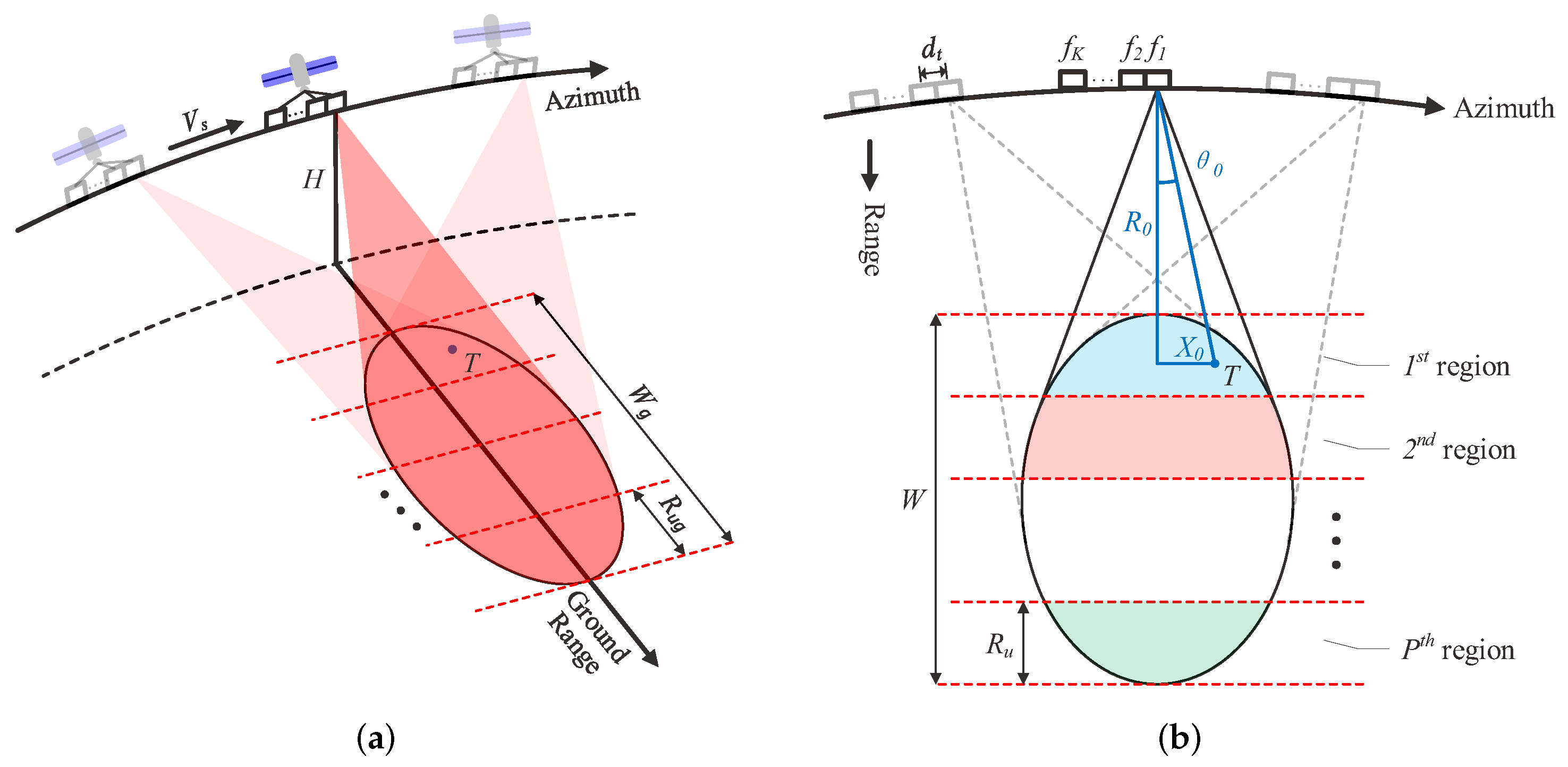
2.1. Geometry and Signal Model

A general illustration of the illumination geometry of a space-borne FDA-SAR working in side-looking spotlight mode is shown in Figure 1. The SAR platform moves along a line in the azimuth direction with a velocity of V s at an altitude of H. During the formation of the spotlight aperture, the antenna is constantly steered to the scene center’s direction. Unlike conventional spotlight SARs, the transmission antenna consists of K channels spaced at a small distance d t along the azimuth direction, and one antenna channel is used for echo receiving.
Let k denote a specific channel, where 1 k K . Taking the first channel as reference, the carrier frequency of the k-th channel is f k = f 0 + ( k 1 ) Δ f , where f 0 is the reference frequency, and Δ f is the frequency increment, which satisfies Δ f f 0 , Δ f B , with B denoting the system bandwidth. The observed swath in the slant range direction is W, while R u is the maximum unambiguous slant range. W g and R u g are their projections on ground. The transmitted signals from the K channels are orthogonal to one another. Reflected by the ground scatterers, the echoes are received by one reception channel. R 0 is the closest range of a scattering point T. Taking the scene center as the azimuth axis origin, X 0 is the azimuth position of T, while θ 0 ( η ) is the instantaneous azimuth angle of T, where η is the slow time. Notate the echo of the k-th transmitted channel signal with s k ( τ , η ) . Ignoring the motion error, the echo signal of T can be expressed as s 0 ( τ , η ) = k = 1 K s k ( τ , η ) , where τ denotes the fast time. After down conversion, the signal is fed into K matched filters to separate the transmitted signal. The output of the k-th filter is:
s k ( τ , η ) = ξ w r , k ( τ t k ( η ) ) · exp { j π K r ( τ t k ( η ) ) 2 } · exp j 2 π f k R t , k ( η ) + R r ( η ) c
where ξ denotes the complex amplitude, w r , k ( τ ) is the range envelope of the base-band signal, K r is the chirp rate of the transmitted linear frequency modulated (LFM) signal, and t k ( η ) is the echo round-trip time delay of the target T. R t , k ( η ) is the instantaneous distance between T and the k-th transmission channel, R r ( η ) is that between T and the reception one, and c is the speed of light.
In a general space-borne SAR system, the far-field and spatial narrow-band assumptions are satisfied [9]. On this foundation, some approximations can be made as follows. In the first place, the instantaneous azimuth angles between T and different equivalent phase centers (EPC) are the same, and are expressed using θ 0 , k ( η ) = θ 0 ( η ) , k = 1 , 2 , , K . In addition, a geometry approximation can be made, namely R t , k ( η ) + R r ( η ) 2 R r e f ( η ) ( k 1 ) d t sin ( θ 0 ( η ) ) , R r e f ( η ) = R 0 2 + ( V s η X 0 ) 2 is the instantaneous slant range between T and the reference EPC. Thirdly, the variance of the round-trip time among channels can be ignored for the echo envelope and the LFM phase term. Thus, we have t k ( η ) t 1 ( η ) = 2 R r e f ( η ) / c .
Taking these approximations into consideration, (1) can be expanded as:
s k ( τ , η ) ξ w r ( τ t 1 ( η ) ) exp { j π K r ( τ t 1 ( η ) ) 2 } × exp j 4 π R r e f ( η ) λ × exp j 2 π ( k 1 ) 2 Δ f d t sin ( θ 0 ( η ) ) c × exp j 4 π ( k 1 ) Δ f R 0 c × exp j 2 π ( k 1 ) d t sin ( θ 0 ( η ) ) λ .
In this equation, λ = c / f 0 is the wavelength of the signal. The first phase term is the LFM term, the second is related to the slow time, the third is the intersected term of the frequency increment and the azimuth angle and can be neglected, while the last two terms vary with the transmission channel and are caused by the FDA structure. The transmission steering vector can be defined as [10]:
T = 1 exp j 4 π Δ f R c + j 2 π d t sin ( θ ) λ exp j 4 π ( k 1 ) Δ f R c + j 2 π ( k 1 ) d t sin ( θ ) λ
where R is the closest slant range and θ is the azimuth angle. According to the form of (3), we define the transmission space frequency as:
f t = 2 Δ f R c + d t sin ( θ ) λ .
In this expression, the independent variables are omitted for clarity.
Using Figure 1b, the azimuth angle θ 0 ( η ) can be calculated as:
θ 0 ( η ) = arcsin X 0 V s η R 0 2 + ( X 0 V s η ) 2 .

2.2. Range Ambiguity Analysis of Spotlight FDA-SAR Echoes

When the round-trip time difference among the echoes from different range regions is an integer multiple of the pulse repetition interval, the echoes would be collected during the same reception window, which would cause range ambiguity. As in Figure 1b, if the desired observed swath W exceeds the maximum unambiguous range R u = c / ( 2 P R F ) in the slant range direction, the range ambiguity would seriously affect the imaging results. The echoes of any two scatterers at a distance of R u overlap in the time domain. We define the range ambiguity number as P = W / R u , that is to say, the swath is divided into P regions. We take the first region where scatterer T is located in as reference and order the range regions with the indices p = 1 , 2 , , P . Considering the scatterers with the same azimuth angle as T and located at the slant range of R = R 0 + ( p 1 ) R u , p = 1 , 2 , , P , their transmission frequency can be expressed as:
f t , p = 2 Δ f ( R 0 + ( p 1 ) R u ) c + d t sin ( θ 0 ) λ .
Generally, the echoes of these scatterers are collected during the same reception window.
From (6), we see that the signals of the scatterers discussed above are separated by a frequency interval Δ f t = 2 Δ f R u / c in the transmission space frequency domain, even if they overlap in the time domain. According to [9], to maximize the space between two adjacent range regions, the frequency increment of the FDA should be set as Δ f = ( N + 1 / P ) P R F , N N , which distributes the different range region and echoes uniformly in the space frequency domain.

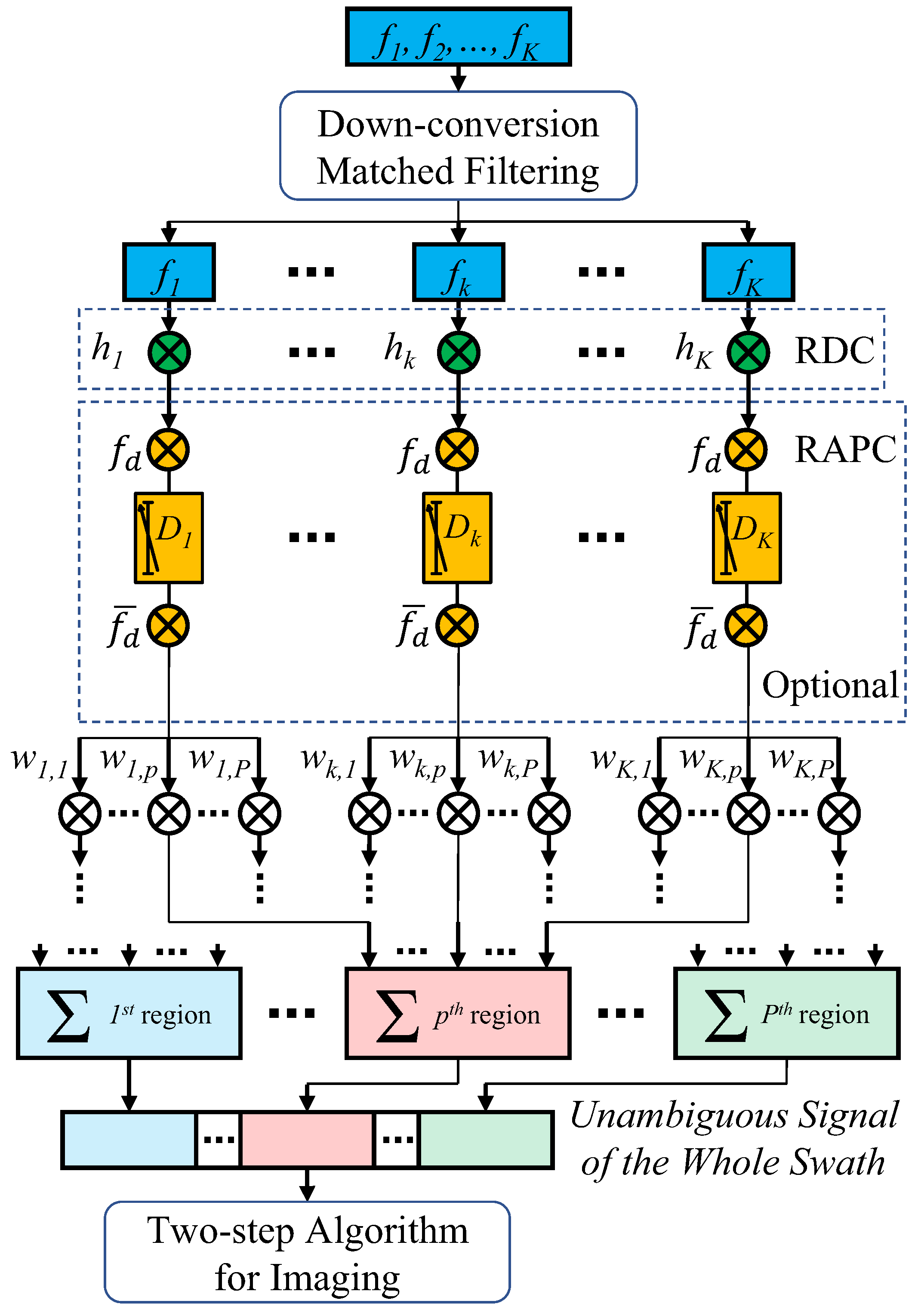
2.3. Range Ambiguity Resolution Approach for Spotlight FDA-SAR

In this section, a time-domain processing method is proposed to resolve the range ambiguity of spotlight FDA-SAR. A basic processing flow is given for general cases and a compensation procedure is put forward to handle large azimuth beamwidth situations.
According to the above analysis, the ambiguous echo signal from the k-th filter containing the scatter from T is formulated as:
s a , k ( τ , η ) = p = 1 P s k , p ( τ , η ) = p = 1 P δ p ( τ , η ) × exp j 4 π ( k 1 ) Δ f ( R 0 + ( p 1 ) R u ) c × exp j 2 π ( k 1 ) d t sin ( θ 0 ( η ) ) λ
where δ p ( τ , η ) = ξ w r ( τ t 1 ( η ) ) · exp { j π K r ( τ t 1 ( η ) ) 2 } · exp j 4 π R p , r e f ( η ) / λ denotes the signal of a traditional spotlight SAR illuminating the p-th range region, while R p , r e f ( η ) represents the slant range of the targets in this region, whose echoes are overlapped with T.

2.3.1. Range Dependence Compensation

From (6), the transmission frequency bandwidth depends on three variables, namely the range region, the range cell, and the azimuth angle. Range dependence compensation (RDC) is used to eliminate the dependence of the range cell, which is implemented through a set of time-domain mixers. The compensating function for the k-th filter output signal is:
h k = exp j 4 π ( k 1 ) Δ f R 0 c .
The signal after RDC is s R D C , k ( τ , η ) = s a , k ( τ , η ) · h k , which can be expanded to:
s R D C , k ( τ , η ) = p = 1 P δ p ( τ , η ) exp j 4 π ( k 1 ) Δ f ( p 1 ) R u c × exp j 2 π ( k 1 ) d t sin ( θ 0 ( η ) ) λ .
The transmission frequency then becomes f R D C , t , p = 2 Δ f ( p 1 ) R u / c + d t sin ( θ 0 ) / λ .

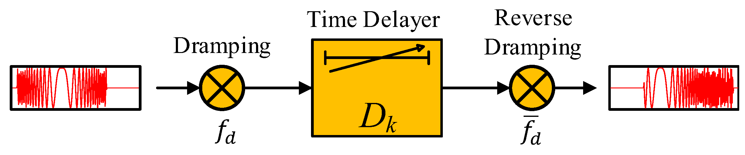
2.3.2. Time-Domain Transmission Beamforming

As discussed above, the ambiguous signals are separated by intentionally designing the frequency increment and implementing RDC. To extract the desired signal, a transmission beamformer is used to enhance the desired signal and remove the ambiguous signals. Thus, the minimum variance distortionless response adaptive beamforming algorithm is used to obtain the weighting vector [7]. Notate the desired observing region with p 1 , and it can be any one of all the range regions. To minimize the ambiguity to signal ratio of the p 1 -th range region, the beamforming weighting factors can be obtained by solving the following optimization problem:
min w p 1 w p 1 H R p 1 w p 1 s . t . w p 1 T R D C = 1 .
where w p 1 is the weighting vector, R p 1 is the covariance matrix of the ambiguity signal, and T R D C is the transmitting vector after RDC. FDA-SAR resolves the range ambiguity by exploiting the degrees of freedom. To reconstruct the signal of W, the number of transmission channels K is constrained to not be less than the range ambiguity number P. If K = m P , m N + , the optimal weighting function of the p 1 -th region and the k-th filter output signal can be defined as w k , p 1 = exp { j 2 π ( k 1 ) f R D C , t , p 1 } , where p 1 = 1 , 2 , , P .
In strip-map mode, the SAR antenna illuminates the ground with a constant squint angle. Accordingly, the scatterers have the same Doppler histories, except for the edge ones as shown in the strip-map mode time-frequency relation map of Figure 2a. B a is the Doppler bandwidth and f η is the frequency axis. Therefore, for the traditional strip-map mode FDA-SAR, the transmission beamformer is required to be designed in azimuth frequency domain to weight the echoes of scatterers simultaneously. However, in spotlight mode, all the scatterers in the scene are distinctive in terms of the Doppler histories. However, they experience the same illumination period as shown in the time-frequency relation map of Figure 2b. The same slow time histories of the scatterers make it feasible to design the transmission beamformer in slow time domain for spotlight FDA-SAR as follows.
Using Figure 1b, in the case of a small azimuth beam width, considering the azimuth center of the scene, the azimuth angle history is θ c ( η ) = arcsin V s η / R 0 2 + ( V s η ) 2 . Accordingly, the weighting function can be expressed as:
w k , p 1 = exp j 4 π ( k 1 ) Δ f ( p 1 1 ) R u c + j 2 π ( k 1 ) d t V s η λ R 0 2 + ( V s η ) 2 .
Applying the weighting filters on (9), the unambiguous signal from the p 1 -th region is reconstructed as s u , p 1 = k = 1 K s R D C , k ( τ , η ) · w k , p 1 , which is expanded as:
s u , p 1 = δ p 1 ( τ , η ) · 1 exp { j φ ( η ) · K } 1 exp { j φ ( η ) } + p = 1 , p p 1 P δ p ( τ , η ) · 1 exp j 4 π Δ f ( p 1 p ) R u c + φ ( η ) · K 1 exp j 4 π Δ f ( p 1 p ) R u c + φ ( η )
where φ ( η ) = 2 π d t λ ( X 0 V s η R 0 2 + ( X 0 V s η ) 2 + V s η R 0 2 + ( V s η ) 2 ) is negligible. Under the condition of Δ f = P R F / P , (12) can be simplified to s u , p 1 = K · δ p 1 ( τ , η ) , which is the exact unambiguous signal of the scatterer overlapped with T, and it is from the p 1 -th region.
T is regarded as a general scattterer in the reference region, similar to the above processing, the unambiguous echoes of all the scatterers from P regions can be reconstructed. Reorganizing them in the range direction, the whole swath signal becomes s u , W = s u , 1 s u , 2 s u , P .
So far, different from the strip-map FDA-SAR, our reconstruction method has been entirely carried out in the time domain. In the case of a small azimuth beam width, the above procedures are sufficient to allow the extension of the range swath, and we name them the central area time-domain processing. An HRWS image can then be generated utilizing the subsequent two-step algorithm [13] used in spotlight SARs.

2.4. Residual Angle Phase Compensation

Being a function of slow time, the ignored term φ ( η ) in (12) varies with the position of the scatterers. When a large azimuth beam width is used, φ ( η ) should be taken into account to ensure the accuracy of the approach.
Let us assume that T is located at the azimuth edge of the scene. Notate the additional term in (12) as ψ p ( η ) , namely:
ψ p ( η ) = 1 exp j 4 π Δ f ( p 1 p ) R u c + φ ( η ) · K 1 exp j 4 π Δ f ( p 1 p ) R u c + φ ( η ) .
For an azimuth edge scatterer, this term remains part of the ambiguity energy. The factor φ ( η ) needs to be compensated to increase the performance.
Applying the approximation sin ( θ 0 ( η ) ) ( X 0 V s η ) / R 0 to φ ( η ) , we have φ 2 π d t X 0 / ( λ R 0 ) , which is independent of slow time. Subsequently, residual angle phase compensation (RAPC) should be applied before the transmission beamforming to remove the ambiguity entirely. For the k-th channel signal, the compensating factor is formulated as:
Δ k = exp { j ( k 1 ) φ } = exp j 2 π ( k 1 ) d t X 0 λ R 0 .
To deal with every scatterer in the scene, signal separation in azimuth is required before compensation. Regarding the azimuth echo as an LFM signal with a chirp rate of K r o t = 2 V r 2 / ( λ R 0 ) , where V r is the equivalent radar velocity, a deramping function of f d = exp { j π K r o t η 2 } can be used to coarsely focus the signals in azimuth [13]. The time-frequency relation after deramping is illustrated in Figure 2c where B a , d e r a m p is the Doppler bandwidth after deramping. Echoes of scatterers have been separated in azimuth frequency domain after deramping. The echo of scatterer T will be focused at the azimuth position of f η , T = K r o t X 0 / V s after the pursuant FT. Replacing f η , T into (14), the frequency-domain form of Δ k becomes:
Δ k = exp j 2 π ( k 1 ) d t f η , T V s λ R 0 K r o t .
Then, we multiply the factor with the signal in the azimuth frequency domain. After transforming the signal into time domain via an inverse FT (IFT), the signal should be restored using the conjugate of the deramping function. The derivation is based on a single scatterer, and f η , T can be extended to the f η axis to handle the signals from the whole scene.
Note that the factor Δ k multiplied with the signal in azimuth frequency domain is a linear phase of f η . Hence, according to the properties of FT, a time delay in azimuth time domain can be adopted to replace the frequency-domain processing to accomplish RAPC. In light of (15), the relative time delay is:
D k = ( k 1 ) d t V s λ R 0 K r o t .
The above analysis means that the RAPC procedure can be carried out in azimuth time domain with a series of mixers and time delayers as the following flow chart in Figure 3.
The complete processing flow chart of our scheme is shown in Figure 4. Apparently, all the procedures of the proposed scheme are carried out in the time domain. The system relies on numerous time mixers in Figure 4, but in an actual hardware system, mixers can be combined for simplification. To discuss the computation load of our scheme, we compared the required number of devices and operations of our scheme and the strip-map FDA-SAR scheme in practice, including mixers, delayers, and FTs/IFTs operations. The results are listed in Table 1.
As in Table 1, identical to the strip-map frequency-domain method, ( K + K · P ) mixers are used in the proposed scheme with or without RAPC, while the difference is that FTs/IFTs are avoided, which brings the possibility of onboard real-time space-borne application. The RAPC approach merely requires extra K delayers, which is easy to achieve in hardware. As for a strip-map FDA-SAR, one X-point radix-2 fast-FT operation needs X · log 2 X complex additions and X 2 · log 2 X complex multiplications. For the space-borne SAR system with a huge size of data, K + 1 FTs/IFTs make it difficult to realize real-time processing in the case. Therefore, even fewer devices and procedures are required in the proposed scheme than that for the conventional strip-map mode FDA-SAR.

2.5. Performance Analysis

The distributed range ambiguity to signal ratio (DRASR) is used to quantitatively evaluate the performance of the proposed scheme. DRASR is defined as the ratio of the ambiguity signal energy to the expected signal energy at each sampling point during the echo reception window. Considering a target T 1 in region p 1 with the position ( R 1 , X 1 ) , the DRASR can be expressed as:
D R A S R = S a , R 1 S R 1
where S a , R 1 and S R 1 are the ambiguity and expected signal energy at slant range R 1 respectively. Regarding the p 1 -th region as the expected observing region, echo signal after the central area time-domain processing without RAPC is shown in (12). Subsequently, the signal energies can be briefly described as:
S a , R 1 ( η ) = p = 1 p p 0 P σ p · G p 2 · | ψ p ( η ) | [ R 1 + ( p p 1 ) R u ] 3 · sin α p S R 1 ( η ) = σ T 1 · G T 1 2 · | ψ p 1 ( η ) | R 1 3 · sin α T 1
where σ T 1 is the normalized scattering coefficient, G T 1 2 is the round-trip range antenna pattern, and α T 1 is the incident angle of T 1 . Additionally, σ p , G p 2 , and α p are the factors of the scatterers in the p-th region, whose echoes were collected at the same time with T 1 .
Apparently, for the azimuth center scatterers, we have ψ p ( η ) = 0 , p p 1 and ψ p 1 = K , DRASR being 0. Therefore, the ambiguity signal is totally removed with central area time-domain processing, even without RAPC.
For the azimuth edge scatterers, RAPC is adopted. After this, the additional term of (12) turns to:
ψ p R A P C ( η ) = 1 exp j 4 π Δ f ( p 1 p ) R u c + φ ( η ) φ · K 1 exp j 4 π Δ f ( p 1 p ) R u c + φ ( η ) φ .
With the residual angle phase compensated mostly, the DRASR value decreases, and the ambiguity signal energy is further attenuated. Note that little residual angle phase remains due to the angle approximation, and it is related with the azimuth position. Therefore, with the DRASR evaluation after RAPC, the azimuth size of the unambiguous swath can be revealed in a specific space-borne SAR system.

3. Simulation Results

3.1. Simulation Parameters

In this section, a simulation experiment of a space-borne spotlight FDA-SAR is implemented to demonstrate the effectiveness of the proposed scheme. The system parameters are listed in Table 2. As shown in Figure 5, the observed swath was divided into 3 regions along the range direction, each with a width of R u , which is exactly the width of the maximum unambiguous range. Several scatterers were distributed in the different regions. These scatterers were divided into areas A, B, and C in azimuth-center of the observed swath, and D, E, and F in azimuth-edge. Scatterers in azimuth center and edge areas were used to demonstrate the performance of the central area time-domain processing and the RAPC approach, respectively.

3.2. Central Area Time-Domain Processing

The imaging results of the azimuth-center areas A, B, and C before and after using the proposed central area time-domain processing without RAPC are compared in Figure 6. To analyze in further detail and demonstrate the range ambiguity resolution performance, the up-sampled amplitude contour maps of scatterer T c are shown in Figure 7. Without the central area time-domain processing, the imaging results in Figure 6a,c,e show serious ambiguity. Whereas, with processing, Figure 6b,d,f shows the clear images with the range ambiguity resolved.

3.3. RAPC

To verify the RAPC approach, the imaging results of the azimuth-edge areas D, E, and F before and after applying the central area time-domain processing and RAPC approach are compared in Figure 8. The scatterer T e in azimuth-edge area D was analyzed with up-sampled amplitude contour maps as Figure 9. Compared with the unprocessed imaging result of Figure 8a,d,g, the central area time-domain processing result of Figure 8b,e,h indicates that the ambiguity was just partially removed, which is not sufficient for edge scatterer imaging. With the RAPC procedure implemented, the residual ambiguity was entirely removed as Figure 8c,f,i.

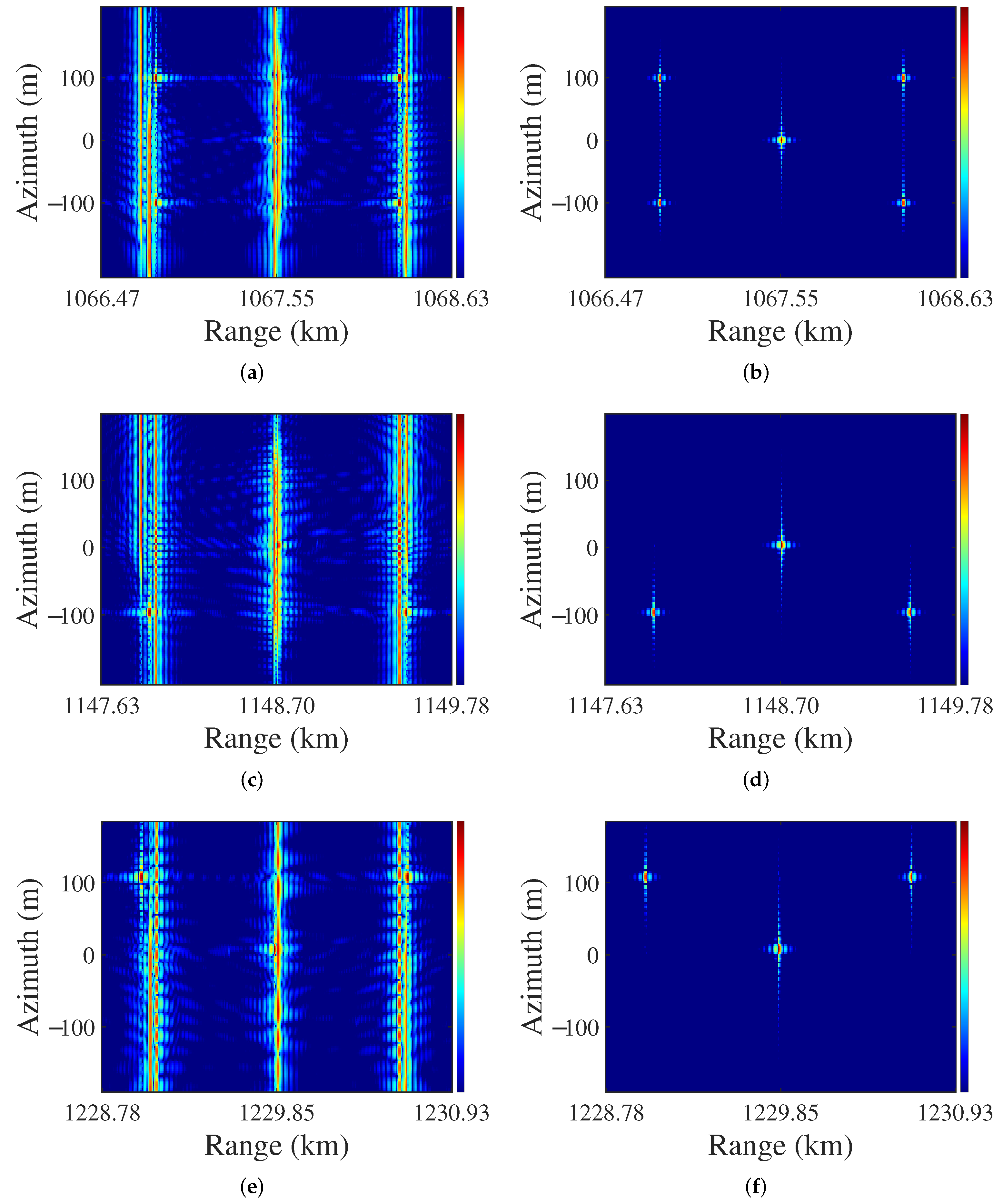
3.4. Performance Analysis

For a general space-borne SAR, the DRASR value of system is commonly required to be less than 20 dB. To quantitatively evaluate the performance of the proposed scheme, we analyzed the DRSAR of 2 groups of areas in azimuth center and edge. As (18), the scattering coefficient σ and round-trip range antenna pattern G 2 are fundamental to the DRASR value. For more intuitive comparison, we set σ and G 2 as constant values. For central areas, the scatterer T c in A and the relative overlapped scatterers in B and C are applied for calculation. In spotlight mode, the range and incident angle vary with the slow time during the whole sampling period. Hence, as (18), the DRASR value is also the function of the slow time as in Figure 10. As exhibited in the diagram, the DRASR values of A, B, and C are around 65.6 dB, 62.2 dB, and 60.1 dB. Thus, for all the 3 central areas in different regions, the ambiguity energy was removed with the central area time-domain processing.
For azimuth-edge areas D, E, and F, after the central area time-domain processing, the DRASR values were around −1.7 dB, 0.7 dB, and 3.5 dB as shown in Figure 11a, which means the range ambiguity seriously influenced the image quality. However, with the additional RAPC approach implemented after RDC, the DRASR values decreased to a range from 65 dB to 40 dB.
For individual analysis, here G 2 was set as a constant. Note that purposely designing the antenna patterns is a general way to suppress the range ambiguity. Echo energies from ambiguous range regions are weighted by the antenna patterns and suppressed. Therefore, even better performance can be obtained with the real antenna patterns combined with the proposed spotlight FDA-SAR scheme.
To evaluate the imaging performance, the point target focusing analysis of the spotlight FDA-SAR scheme is in Table 3. In Figure 5, we selected one point target in each of the six areas from A to F for analysis. Peak side-lobe ratio (PSLR), integral side-lobe ratio (ISLR), and impulse response width (IRW) were analyzed here. The ideal IRW was normalized to 0.886. Point targets T e , E 1 , and F 1 at azimuth edge were processed with additional RAPC approach. The results indicate that all the six point targets were well focused. This also demonstrates the removal of the range ambiguity.

3.5. Conventional Approach

To prove the necessity of processing being implemented in the time domain for a spotlight FDA-SAR system, we used the conventional strip-map frequency-domain method to handle the ambiguous signal of the region A, B and C. For contrast with Figure 6b,d,f, the imaging results are shown in Figure 12. Distinctly, the frequency-domain method failed to remove the ambiguity. Note that here, the ambiguity problem will get worse when the steering angle is increased.

4. Discussion

Due to disparate illumination geometries, the Doppler histories of scatterers in strip-map and spotlight mode are essentially different. As results, the conventional range ambiguity resolution for strip-map FDA-SAR is not available for spotlight mode, even for central areas. As in Figure 12, with conventional frequency-domain processing, range ambiguity still remains. In actual images, it is hard to recognize the real targets.
Range ambiguity occurs when the echoes from different range regions arrive at the signal receiver concurrently. To be clear, the ambiguity signal in one region was from the other two regions. As in Figure 6, locating at the azimuth center, the expected signal was extracted from the ambiguity merely with central area time-domain processing. The contour maps of T c in Figure 7 show that the ambiguity signal amplitude decreased under 30 dB. Furthermore, the DRASR values in Figure 10 and point analyses in Table 3 also confirmed the elimination of range ambiguity. For central areas, the residual angle phase in (12) is too small to deactivate the transmission beamformer, and it is negligible. Therefore, central area time-domain processing can handle the situation with a small azimuth beamwidth.
The central area time-domain processing still has limitations when it comes to a large azimuth beam width. Figure 8 shows that it is not sufficient for edge scatterer imaging. Residual angle phase remained partial ambiguity energy, as in Figure 9b. Implementing the RAPC approach, Figure 9c gives the clear image.
In terms of the system complexity, based on the processing flow chart in Figure 4, numerous mixers can be combined. To contrast with the strip-map FDA-SAR, fewer devices are needed, which turns to an advantage of the proposed scheme.
For a space-borne SAR system, the proposed scheme in this paper broadens the range swath on the basis of inheriting azimuth high resolution of spotlight mode. Implemented in frequency domain, strip-map FDA-SAR processing generally consumes large computational resources, which is unrealistic for real-time processing. However, entirely carried out in the time domain, our proposed scheme has high computing efficiency and can be realized onboard in real-time. In addition, it is feasible to integrate it into other real-time approaches. The case in point is the real-time digital beamforming technology, which is also based on the multichannel system. On the premise of HRWS capability, the signal-to-noise ratio of the image can be improved concurrently.
The case of a spotlight FDA-SAR working with a large squint angle will be considered in our future work, the approximation of azimuth angle is invalid in that case. The foundation of the time-domain processing is the same slow time histories of all scatterers in the swath. Without the property, for other SAR modes, like slide spotlight SAR, TOP-SAR, or Mosaic SAR, the FDA technique needs to be improved and optimized to combine with them. To expand the compatibility, our future work will deal with these situations.
FDA-SAR system resolves the range ambiguity with few onboard resources. However, the research on it is still in the stage of theoretical derivation. Some challenges still restrict the application of FDA-SAR system in practice, of which the typical one is the orthogonal waveform characteristics of the transmitted signal being difficult to accurately satisfy. This will lead to deterioration of range ambiguity resolution performance. Therefore, designing orthogonal waveform transmitted signals and reducing correlation among them will be the focus of future research. At present, some representative potential solutions include the orthogonal-waveform beamforming scheme [14], the echo separation scheme based on orthogonal frequency-division multiplexing (OFDM) chirp waveforms [15], and the segmented phase coding scheme [16] et al.

5. Conclusions

In this study, a novel unambiguous signal reconstruction scheme for a spotlight FDA-SAR is presented. It is featured being implemented in the time domain. Based on the theoretical derivation and simulation verification presented, the following conclusions can be drawn. Time-domain processing makes the proposed spotlight FDA-SAR model more efficient than strip-map mode operation. For space-borne SAR systems, the proposed time-domain processing can be combined with other real-time algorithms. The spotlight FDA-SAR still inherits the high azimuth resolution performance of the conventional spotlight SAR when the unambiguous range swath is broadened. In addition, the proposed scheme is designed with spatial variability in azimuth, which allows handling of cases with a large azimuth beam width.

Author Contributions

Conceptualization, Y.W. and Z.C.; investigation, Z.Z.; methodology, Y.W.; validation, Y.W. and M.R.; formal analysis, Y.W.; data curation, X.M. and J.Q.; writing—original draft preparation, Y.W.; writing—review and editing, Y.W. and Z.C. All authors have read and agreed to the published version of the manuscript.

Funding

This work was funded by the National Natural Science Foundation of China under grant numbers 61971401 and 61901442.

Institutional Review Board Statement

Not applicable.

Informed Consent Statement

Not applicable.

Data Availability Statement

Not applicable.

Conflicts of Interest

The authors declare no conflict of interest.

References

  1. Moreira, A.; Prats-Iraola, P.; Younis, M.; Krieger, G.; Hajnsek, I.; Papathanassiou, K.P. A tutorial on synthetic aperture radar. IEEE Geosci. Remote Sens. Mag. 2013, 1, 6–43. [Google Scholar] [CrossRef]
  2. Mittermayer, J.; Moreira, A.; Loffeld, O. Spotlight SAR data processing using the frequency scaling algorithm. IEEE Trans. Geosci. Remote Sens. 1999, 37, 2198–2214. [Google Scholar] [CrossRef]
  3. Antonik, P.; Wicks, M.; Griffiths, H.; Baker, C. Frequency diverse array radars. In Proceedings of the 2006 IEEE Conference on Radar, Verona, NY, USA, 24–27 April 2006; pp. 215–217. [Google Scholar] [CrossRef]
  4. Antonik, P.; Wicks, M.C.; Griffiths, H.D.; Baker, C.J. Range-dependent beamforming using element level waveform diversity. In Proceedings of the 2006 International Waveform Diversity Design Conference, Lihue, HI, USA, 22–27 January 2006; pp. 1–6. [Google Scholar] [CrossRef]
  5. Secmen, M.; Demir, S.; Hizal, A.; Eker, T. Frequency Diverse Array Antenna with Periodic Time Modulated Pattern in Range and Angle. In Proceedings of the 2007 IEEE Radar Conference, Waltham, MA, USA, 17–20 April 2007; pp. 427–430. [Google Scholar] [CrossRef]
  6. Farooq, J.; Temple, M.A.; Saville, M.A. Exploiting frequency diverse array processing to improve SAR image resolution. In Proceedings of the 2008 IEEE Radar Conference, Rome, Italy, 26–30 May 2008; pp. 1–5. [Google Scholar] [CrossRef]
  7. Xu, J.; Zhu, S.; Liao, G. Range Ambiguous Clutter Suppression for Airborne FDA-STAP Radar. IEEE J. Sel. Top. Signal Process. 2015, 9, 1620–1631. [Google Scholar] [CrossRef]
  8. Xu, J.; Liao, G.; So, H.C. Space-Time Adaptive Processing with Vertical Frequency Diverse Array for Range-Ambiguous Clutter Suppression. IEEE Trans. Geosci. Remote Sens. 2016, 54, 5352–5364. [Google Scholar] [CrossRef]
  9. Wang, C.; Xu, J.; Liao, G.; Xu, X.; Zhang, Y. A Range Ambiguity Resolution Approach for High-Resolution and Wide-Swath SAR Imaging Using Frequency Diverse Array. IEEE J. Sel. Top. Signal Process. 2017, 11, 336–346. [Google Scholar] [CrossRef]
  10. Lin, C.; Huang, P.; Wang, W.; Li, Y.; Xu, J. Unambiguous Signal Reconstruction Approach for SAR Imaging Using Frequency Diverse Array. IEEE Geosci. Remote Sens. Lett. 2017, 14, 1628–1632. [Google Scholar] [CrossRef]
  11. Chen, Z.; Zhang, Z.; Zhou, Y.; Zhao, Q.; Wang, W. Elevated Frequency Diversity Array: A Novel Approach to High Resolution and Wide Swath Imaging for Synthetic Aperture Radar. IEEE Geosci. Remote Sens. Lett. 2020, 19, 1–5. [Google Scholar] [CrossRef]
  12. Zhou, Y.; Wang, W.; Chen, Z.; Zhao, Q.; Zhang, H.; Deng, Y.; Wang, R. High-Resolution and Wide-Swath SAR Imaging Mode Using Frequency Diverse Planar Array. IEEE Geosci. Remote Sens. Lett. 2021, 18, 321–325. [Google Scholar] [CrossRef]
  13. Fornaro, G.; Lanari, R.; Sansosti, E.; Tesauro, M. A two-step spotlight SAR data focusing approach. In Proceedings of the IGARSS 2000. IEEE 2000 International Geoscience and Remote Sensing Symposium. Taking the Pulse of the Planet: The Role of Remote Sensing in Managing the Environment. Proceedings (Cat. No.00CH37120), Honolulu, HI, USA, 24–28 July 2000; Volume 1, pp. 84–86. [Google Scholar] [CrossRef]
  14. Rommel, T.; Rincon, R.; Younis, M.; Krieger, G.; Moreira, A. Implementation of a MIMO SAR Imaging Mode for NASA’s Next Generation Airborne L-Band SAR. In Proceedings of the EUSAR 2018, 12th European Conference on Synthetic Aperture Radar, Aachen, Germany, 4–7 June 2018; pp. 1–5. [Google Scholar]
  15. Kim, J.H.; Younis, M.; Moreira, A.; Wiesbeck, W. A Novel OFDM Chirp Waveform Scheme for Use of Multiple Transmitters in SAR. IEEE Geosci. Remote Sens. Lett. 2013, 10, 568–572. [Google Scholar] [CrossRef]
  16. Jin, G.; Deng, Y.; Wang, W.; Wang, R.; Zhang, Y.; Long, Y. Segmented Phase Code Waveforms: A Novel Radar Waveform for Spaceborne MIMO-SAR. IEEE Trans. Geosci. Remote Sens. 2021, 59, 5764–5779. [Google Scholar] [CrossRef]
Figure 1. Illumination Geometry of Spotlight FDA-SAR. (a) In spatial coordinate system. (b) In azimuth-range plane coordinate system.
Remotesensing 14 01085 g001
Figure 2. Time-frequency diagrams of the signal in strip-map mode and spotlight mode. (a) Strip-map mode. (b) Spotlight mode before deramping. (c) Spotlight mode after deramping.
Remotesensing 14 01085 g002
Figure 3. Residual angle phase compensation approach.
Remotesensing 14 01085 g003
Figure 4. Processing flow chart of the spotlight FDA-SAR imaging scheme.
Remotesensing 14 01085 g004
Figure 5. Distributions of scatterers.
Remotesensing 14 01085 g005
Figure 6. Imaging results of areas A, B, and C with and without the central area time-domain spotlight FDA-SAR range ambiguity resolution. (a) Area A, without processing. (b) Area A, with processing. (c) Area B, without processing. (d) Area B, with processing. (e) Area C, without processing. (f) Area C, with processing.
Remotesensing 14 01085 g006
Figure 7. Up-sampled contour map of the scatter T c in azimuth-center area A. (a) Without processing. (b) With central area time-domain spotlight FDA-SAR ambiguity resolution.
Remotesensing 14 01085 g007
Figure 8. Imaging results of azimuth-edge area D, E, and F. (a) Area D, without processing. (b) Area D, with central area time-domain processing. (c) Area D, with additional RAPC. (d) Area E, without processing. (e) Area E, with central area time-domain processing. (f) Area E, with additional RAPC. (g) Area F, without processing. (h) Area F, with central area time-domain processing. (i) Area F, with additional RAPC.
Remotesensing 14 01085 g008
Figure 9. Up-sampled contour map of the scatter T e in azimuth-edge area D. (a) Without processing. (b) With central area time-domain spotlight FDA-SAR range ambiguity resolution. (c) With additional RAPC processing.
Remotesensing 14 01085 g009
Figure 10. DRASR of area A, B, and C with central area time-domain processing.
Remotesensing 14 01085 g010
Figure 11. DRASR of area D, E, and F with central area time-domain processing and additional RAPC processing. (a) With central area time-domain processing. (b) With additional RAPC processing.
Remotesensing 14 01085 g011
Figure 12. Imaging results of area A, B, and C in spotlight mode using conventional range ambiguity resolution for strip-map FDA-SAR.
Remotesensing 14 01085 g012
Table 1. Required number of devices and operations.
SchemesMixersDelayersFTs/IFTs Operations
Spotlight FDA-SAR without RAPC K + K · P 00
Spotlight FDA-SAR with RAPC K + K · P K0
Strip-map FDA-SAR K + K · P 0 K + 1
Table 2. System Parameters.
ParametersValues
Carrier frequency5.4 GHz
Platform height710 km
Platform velocity7503 m/s
Incident angle45°
Steering angle−1° to 1°
Number of transmission channels6
Antenna size (height × length)10 m × 2 m
Signal bandwidth100 MHz
Sampling frequency133 MHz
Pulse duration5 μ s
PRF1866 Hz
Frequency increment622 Hz
Azimuth beam width0.318°
Table 3. Point Target Imaging Performance.
PointAreaRegionAzimuthRange
 PSLR/dB ISLR/dB IRW PSLR/dB ISLR/dB IRW
T c A1st region−13.24−10.200.886−13.25−10.180.886
B 1 B2nd region−13.26−10.210.887−13.27−10.160.884
C 1 C3rd region−13.28−10.150.885−13.27−10.160.886
T e D1st region−13.26−10.280.885−13.24−10.240.885
E 1 E2nd region−13.24−10.330.886−13.26−10.250.886
F 1 F3rd region−13.27−10.310.886−13.26−10.250.886
Publisher’s Note: MDPI stays neutral with regard to jurisdictional claims in published maps and institutional affiliations.

