Abstract
3-D phase unwrapping (PU) methods based on the 2-D linear temporal coherencemodel have been widely used in time-series interferometric synthetic aperture radar (TS-InSAR) for measuring topography and monitoring subtle deformation. However, the linear temporal coherencemodel can not characterize the coherence of highly coherent pixels accurately in seasonal deformation areas, where nonlinear deformation is deterministic and nonnegligible. Especially, for urban areas with groundwater or thermal dilation seasonal changes or permafrost regions, the nonlinear deformation is usually associated with periodic temperature changes. In this work, a general multi-component temporal coherence model, which considers multiple components including the seasonal deformation, is proposed for 3-D PU of seasonal deformation areas. Moreover, the uncertainty evaluation criterion, based on Cramér–Rao bound (CRB), is derived for TS-InSAR. The experimental results, obtained by applying the multi-component temporal coherence model to a data set acquired from January 2012 to February 2016 over the Beijing Capital International Airport area, confirm the effectiveness of the proposed method. High phase consistency, accurate corrected digital elevation model (DEM) and deformation information monitoring with high-density and high-coverage PS pixels are achieved. Under the same iterations and TS-InSAR procedure, the enhanced performance by the proposed model is illustrated by comparing with that of linear model in terms of phase consistency of 3-D phase unwrapping, PSCs selection at each step, and final results evaluation. In summary, the number of phase-consistency edges after 3-D PU is increased by about 15%, the number of final PS pixels selected with the same coherence threshold constraint is increased by about 10%, and more PS pixels provide a low uncertainty in residual topography, mean deformation velocity and seasonal amplitude estimation.
1. Introduction
Due to the capability of measuring topography up to sub-meter scale and monitoring subtle deformation up to mm/year scale, time series interferometric synthetic aperture radar (TS-InSAR) techniques [1], especially persistent scatterers InSAR (PS-InSAR) [2,3,4,5,6,7], have been widely employed in various remote sensing applications, and even for phase calibration of advanced tomographic SAR imaging [8]. Such deformation and topography information can only be extracted from the unwrapped phase (or absolute phase), and thus, phase unwrapping (PU) is a critical problem in TSInSAR [9].
The PU problem in TS-InSAR is defined on the sparse 3-D grids (2-D in spatial domain and 1-D in temporal domain) rather than on one regular interferogram [10]. The study on efficient and accurate sparse 3-D PU methods has been of crucial importance at the advent of TS-InSAR during the past few decades [11]. 3-D PU methods can be divided into two categories: phase model or simply model based and non-model-based [12].
The non-model-based methods rely on the Itoh condition or phase continuity [13,14], that is, the absolute phase difference between any two neighboring pixels is less than . They unwrap each set of 2-D grids individually using sparse 2-D PU methods [15,16], or two-step 3-D PU methods that unwrap firstly in 1-D temporally (temporal PU, TPU) then in the remaining 2-D spatially (spatial PU, SPU), or jointly unwrap 3-D grids by extending the 2-D PU methods to the 3-D situation. Costantini et al. extended the minimum cost flow (MCF) method to sparse 2-D grids and proposed sparse MCF (SMCF) [15], then individually applied to each 2-D grid for 3-D PU. Hopper resampled the wrapped phase of the sparse grid into a regular grid by a nearest-neighbour interpolation routine, then applied the optimisation routines of SNAPHU [17] to each interferogram, and projected the unwrapped phase into the sparse 3-D grid [16]. Following the strategy, numerous 2-D PU methods based on the phase-continuity assumption, such as, quality-guided [13], branch cut [18], MCF [19] and deep learning [20,21] methods, can be applied by replacing SNAPHU with other 2-D methods. Based on the assumption, Hopper et al. developed a stepwise 3-D PU algorithm that unwrapped phase firstly in 1-D temporally then iteratively improved the solution in the other two dimensions; additionally, they extended the 2-D branch-cut method into the 3-D case and framed 3-D grids PU in terms of an -norm optimization problem [22]. Shanker et al. presented an integer programming formulation which incorporates external measurements as constraints for 3-D grids PU [23]. Costantini et al. formulated the 3-D PU in a common framework [24], which includes standard techniques and constraints from external information if available. Liu et al. established a mathematical constraint within the closure phases and unwrapped sparse 3-D grids jointly [25]. However, these methods are sensitive to deformation or atmospheric signal of long time series and sudden changes of residual topography for low density grid, which results in that the phase continuity assumption is not valid any more. It seems that the joint 3-D PU methods are theoretically the most reliable, but the heavy computational load and long time series as well as low density grid limit their applications [10].
In order to reduce the influence resulting from long time series and low density grid, 3-D PU methods based on the phase model have received many attentions in TS-InSAR. The model-based methods assume that the unmodeled residual phase is subject to the Itoh condition. Firstly, the major component of phase gradients (PGs), such as the differential phase of linear deformation and residual topography, is obtained by maximizing temporal coherence associated with the phase model [2]. Then, the PG of residual phase is unwrapped temporally and then spatially based on the phase continuity assumption [12,26,27]. Pepe and Lanari unwrapped the residual PGs with the extended MCF (EMCF) method in the temporal/baseline plane and then in the azimuth/range plane, and finally the 3-D absolute phase is obtained by spatial integration [26]. Cuenca and hooper et al. took advantage of spatially correlated information to improve the TPU [28]. Fornaro et al. modified the extended SMCF approach so that a more complex network for 3-D PU can be generated and effectively unwrapped [12]. Alternatively, based on the linear phase model associated with the residual topography and mean deformation velocity, Kampes et al. translated TPU of wrapped PGs into a MILS problem weighted by the variance-covariance matrix of the observed phase, and then the phase ambiguities were solved by the LAMBDA technique [29]. Li et al. improved the TPU of PGs by a feasible and practical triangle-oriented TPU strategy based on the linear phase model with the spatial irrotational constraints imposed, and then more reliable unwrapped PGs were obtained by an -norm SPU method with a novel weight function [10]. The model-based methods have great potential for large scale measurement of DEM and deformation both spatially and temporally. However, these methods are mainly for the selected pixels with high coherence, and the modeled phase is assumed to be 2-D linear. In TS-InSAR, the 3D PU is dependent on selection of highly coherent pixels. On the one hand, if the accuracy of 3D PU is poor, the coherence of candidate pixels would not be effectively estimated from the unwrapped phase, and then the identification accuracy of high-coherence pixels is affected. On the other hand, if the low-coherence pixels participate in 3D PU with high-coherence ones, their PU error would inevitably propagate to the latter, although low-coherence pixels are penalized with low weight. Thus, an accurate 3D PU method for sparse grids must consider a constrained integral path, which skips the low-coherence pixels and integrates the phase along the high-coherence pixels [27]. Besides, for seasonal deformation areas, e.g., urban areas where the groundwater changes seasonally or buildings are affected by thermal dilation, or permafrost regions with periodic temperature changes, the 2-D linear model cannot characterize the high-coherence pixels accurately. Then, the coherence of the pixels with great seasonal deformation is underestimated. Moreover, these pixels are dropped innocently due to the high-coherence constraints in 3D PU.
In this work, a general multi-component temporal coherence model, including the 2-D linear component and the seasonal deformation, is proposed for 3-D PU of seasonal deformation areas, such as urban areas where the groundwater changes seasonally or buildings are affected by thermal dilation, or permafrost regions with periodic temperature changes. Then, the uncertainty evaluation criterion, based on Cramér–Rao bound (CRB), is derived for TS-InSAR. We employ the multi-component temporal coherence model and uncertainty criterion for 3-D PU and to evaluate results. To demonstrate the improvement, both conventional linear and multi-component temporal coherence models are applied to PS-InSAR using the same data set, acquired by TerraSAR-X/TanDEM-X over the Beijing Capital International Airport area. A new DEM significantly more accurate than the referred one and deformation information monitoring with high-density and high-coverage PS pixels are achieved. Given the same iterations and TS-InSAR procedure, the enhanced performance by the proposed model is illustrated by comparing with that of the conventional linear temporal coherence model from aspects of 3-D PU evaluation, PS candidates (PSCs) selection at each step and the final estimation results. In summary, the number of final PS pixels selected with the same coherence threshold is increased by about 10%, and more PS pixels provide low uncertainty in residual topography, mean deformation velocity and seasonal amplitude estimation; moreover, a competitive computing speed is achieved.
The rest of this paper is organized as follows. In Section 2, a review of the PS-InSAR and 3-D PU based on EMCF is provided, followed by the proposed multi-component temporal coherence model and uncertainty evaluation criterion for PS-InSAR in Section 3 and Section 4, respectively. The enhanced performance by the proposed model is illustrated by real data experiments in Section 5. Finally, conclusions are drawn in Section 6.
2. PS-InSAR Based on the Linear Temporal Coherence Model
2.1. PS-InSAR
The interferometric phase is composed of several components associated with the acquisition geometry (platform positions and topography), terrain motion, scattering changes (due to temporal variations and/or baseline decorrelation), atmospheric screen delay and orbit errors [2,3]. However, the obtained observations of the i-th interferometric phase at the x-th pixel are wrapped, mathematically,
where is the modulo- operation, is the deformation phase, is delay phase resulting from atmospheric phase screen (APS) and orbit, is the thermal noise phase, and is the residual topography phase after removal of referred topography phase, expressed as
where , r, are SAR wavelength, slant range, incidence angle; and are the i-th perpendicular baseline and residual topography, respectively. Usually, the dominant deformation is modeled linearly,
where and v are the i-th observed time relative to the master observation and mean deformation velocity in line-of-sight (LOS) direction. Thus, the residual unmodeled deformation, also called non-linear deformation, can be expressed by
Then, the coherence model of the x-th pixel is defined by
where , and M represents the number of interferograms. Coherence of the PSCs can measure the stability of phase, and thus is usually used for accurate PS selection [2,3].
Figure 1 presents the flowchart of PS-InSAR. Firstly, the PSCs are selected based on amplitude dispersion . Then, the interferometric phase of PSCs grids is unwrapped temporally and then spatially, and the residual topography and mean deformation velocity are also obtained. Furthermore, the APS and orbit phase and the unmodeled deformation and noise phase are separated based on their different temporal and spatial characteristics [6]. Subsequently, the coherence of each PSCs, used for dropping the unstable PSCs, is estimated by Equation (5). The new iteration begins from 3 to D PU after the PSCs are updated; otherwise, output the results of corrected DEM and mean deformation velocity as well as deformation series.
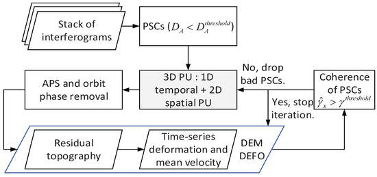
Figure 1.
PSI flowchart.
The improved PS-InSAR (IPSI [7]) relaxes the original PSCs selection condition by , and more PS pixels with stable phase and high precision are selected than that of PS-InSAR. Therefore, the IPSI method is applied in experiment to test the multi-component temporal coherence model and compare it with the 2-D linear model.
2.2. Linear Temporal Coherence Model for 3D PU
For long term and large scale observations, in 3D PU of PS-InSAR, the absolute PGs between adjacent pixels instead of the phases of a single pixel are firstly estimated using TPU methods, and subsequently, the absolute phase gradients are integrated in the space domain. Especially, the neighboring pixel pairs are defined as arcs in a network such as the Delaunay triangulation of the sparse grids.
Since the linear components dominates the major component, and the residual deterministic components and are spatially correlated [2,3,6], the temporal coherence model used for the arcs PGs TPU can be expressed as
where is the differential operator of pixels and . Then, the differential residual topography and deformation velocity of pixels and , and , are estimated by maximizing the temporal coherence,
Then, the modeled phase are obtained, so do the residual topography and deformation velocity of each PSC based on the reweighted LS method.
Consequently, the residual deterministic components are unwrapped in 3-D. Firstly, the residual PGs must be unwrapped temporally [26,27]. The unwrapped PGs can be expressed as follows:
with
where is the unwrapped value of , and is the residual unknown integer number we want to estimate.
The EMCF method for TPU applies the MCF technique to the temporal/baseline grid, and searches for the solution of the following minimization problem [26]
subject to the constraints
where , , and denote the effective arc labels of the Delaunay triangulation network in temporal/baseline plane, , and make a Delaunay triangulation, denotes the differential operator of the -th and -th interferograms, and represents the operation of approximation to the nearest integer number.
With the master one as starting point for TPU, for each arc is obtained by integrating along the Delaunay triangulation network of temporal/baseline plane. Similar to TPU, the SMCF method [15] is extended for SPU [26]. Then, the residual of is obtained. After selecting a high coherent PS as starting point for SPU, for each PSC is obtained by integrating along the Delaunay triangulation network of temporal/baseline plane.
As shown in Figure 2, 3-D PU based on EMCF includes six steps.

Figure 2.
Flowchart of two-step 3D PU based on model.
- Delaunay triangulation network in azimuth/range is formed spatially by PSCs.
- temporal coherence of each arcs in azimuth/range plane is calculated based on model.
- The constrained Delaunay triangulation network in time/baseline plane is formed for TPU.
- TPU is carried out based on the EMCF method.
- The constrained Delaunay triangulation network in azimuth/range plane is formed for SPU.
- SPU is carried out based on the SMCF method.
3. Multi-Component Temporal Coherence Model for TS-InSAR
For long term observations, the seasonal motion is significant since the temperature varies periodically [29,30], especially for permafrost regions or some urban areas influenced by groundwater or thermal dilation. By considering seasonal deformation, the modeled deformation phase can be expressed as [4,29,31]
where sin and cos are base functions of seasonal motion, and is the multi-component modeled phase, including residual topographic, 2-D linear and seasonal components. Multiple components, such as residual topography, deformation velocity and seasonal amplitude, of each pixel are then effectively estimated by time series regression analysis from the unwrapped phase.
As the seasonal component is deterministic and non-negligible in TS-InSAR, the conventional linear coherence model cannot accurately estimate the coherence of pixels. Here we consider introducing the component into the conventional temporal coherence model for 3D PU of seasonal deformation areas. Firstly, a multi-component coherence model is defined as
where is the new unmodeled or residual deformation, excluding the seasonal component, which is included as residual phase in the conventional linear temporal coherence model [2,3,7]. Then, a new temporal coherence model, named the multi-component temporal coherence model, can be written by
which not only includes the linear but also the periodic nonlinear components.
Mathematically, the format of seasonal deformation can be changed as
where is a constant, is seasonal amplitude, and is the initial offset of seasonal motion. Since the seasonal motion is highly correlated with temperature, we can fit certain offset with time series temperature of the observed area. Concretely, we can perform exhaustive search over the optimized range from −1 year to +1 year to maximize the correlation between the monthly average temperature of the studied area with the seasonal deformation model (Equation (15)). It is worth noting that if the temperatures change aperiodically and the seasonal motion is highly correlated with temperature, then the nonlinear deformation model may not be in the trigonometric form as Equation (15). However, the multi-component temporal coherence model can still be applied for other well-established models, such as the thermal dilation model [30]. Since q is a time series constant, after substituting Equations (12) and (15) into (14), the multi-component temporal coherence model can be simplified as
Therefore, the dimension that maximizes the multi-component temporal coherence is reduced from 4 to D to 3-D as
A strategy based on 3-D grid search is used to obtain global solution of the optimization problem. The search is from a coarse to a fine 3-D grid, that is, the 3-D grid is set coarsely to obtain a coarse solution, which is then set as central point of fine grid for further improved solution. In detail, we search first from large ranges [−30 m, 30 m], [−12 mm/yr, 12 mm/yr] and [−5 mm, 5 mm] with large discrete intervals 1 m, 0.5 mm/yr and 0.25 mm, respectively. Then, an initial coarse solution is obtained. We set the coarse solution as central point and search for the fine solution from the small ranges , and with small discrete intervals 0.05 m, 0.025 mm/yr and 0.025 mm, respectively. The computation complexity through this strategy is greatly reduced in comparison to directly searching for the fine solution from a large range with a small discrete interval. However, multidimensional search still leads to a large computational effort. Thus, a fast computing strategy is adopted with Graphics Processing Unit (GPU) computing for 3-D grid search and central processing unit (CPU) paralleling for multiple arcs simultaneously.
With the temporal coherence of each arc calculated in (17) as weight, the residual topography and deformation velocity and seasonal amplitude of each PSC can be estimated by the reweighted LS method [2]. After substituting the estimations into Equation (12), the dominant modeled phase is obtained for 3-D PU.
4. CRB for Performance Evaluation
After removal of residual deterministic components and , which are estimated based on different characteristic behavior in spatial and temporal domains [2,3,6], the unwrapped interferometric phase can be expressed as
where is the parameter vector of TS-InSAR to be estimated, and is the transpose.
On the assumption that the residual deterministic components are fully removed and the noise phase is zero-mean circular Gaussian distributed, the data vector of Equation (18) has mean values of
and the common covariance matrix
where I is the identity matrix, and is the variance of noise phase. Accordingly, the likelihood function of is given by
The Cramér–Rao bound (CRB) can be employed for evaluating the performance of unbiased estimators [32,33,34,35,36,37,38,39,40]. From the Fisher information matrix
we can drive the CRB of estimated variables in TS-InSAR. In detail, from the CRB matrix , the elements , and are uncertainties of the residual topography, deformation velocity and seasonal amplitude, respectively.
With the idealized data statistics described in Equations (18)–(21), the element of Equation (22) can be simplified as [32,33]
where . It is worth mentioning that can be estimated by variance of the time-series noise phase vector . With the independence assumption of estimated variables, Equation (23) is easily calculated according to Equation (19).
5. Study Area and Dataset Used
To assess the 3D PU performance based on the proposed model, the Beijing Capital International Airport site is selected as the study areas, which is marked with red dotted box in Figure 3. The study area, showing seasonal deformation signals [41], is located at Shunyi District, northeast of Beijing, China. There are multiple types of scattering characteristics over the Beijing Capital International Airport site, including complex buildings, runways and roads, which may present thermal-dilation-induced seasonal deformation. Beijing Capital International Airport is mainly composed of three terminals (T1, T2, and T3), and T3 was built in 2008 to cope with the extra traffic brought by the 2008 Olympic visitors. The roof of the T3 C and T3 E building is in a streamlined shape [42].
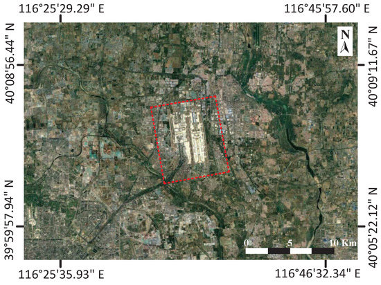
Figure 3.
Shunyi District from Google Earth. The study area is the T3 E building marked with a red rectangles.
The data set covers the Beijing Capital International Airport (Beijing, China) area, and is composed of 31 acquisitions collected by the TerraSAR-X/Tandem-X sensors between January 2012 and February 2016, with a ground area of 8.72 km × 7.3 km. The observing dates and perpendicular baselines and mean monthly temperatures of the 31 passes are summarized in Table 1. The maximum temporal baseline is about 4 years, and the perpendicular baseline ranges from −182 m to 312 m, and the mean monthly temperatures ranges from −7 C to 29 C. The TerraSAR-X image acquired on 10 October 2013 was selected as the master image and the remaining images were jointly co-registered with it. Figure 4 presents the master SAR image (2 m and 1 m for azimuth/range resolution), optical image from Google Earth and the one arc-second (30 m spatial resolution) SRTM DEM used to remove the referred topographic phase, respectively. After removing the derived phase from interferograms, a series of differential interferograms were generated for TS-InSAR.

Table 1.
Details of the used TerraSAR-X/Tandem-X data set, the date shows in the form of year-month-day.
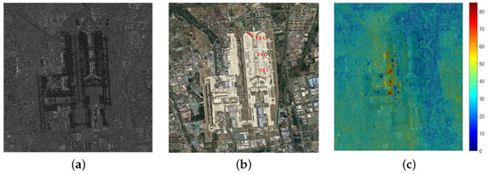
Figure 4.
Beijing Capital International Airport. All images shown with azimuth-slant range coordinates. (a) SAR image; (b) optical image (Google Earth); (c) SRTM DEM with SAR amplitude on the background [m].
Since the SRTM DEM was generated by SAR data collected in February 2000 and T3 of Beijing Capital International Airport was built in March 2004 and finished in November 2007, large residual topography exists in the Beijing Capital International Airport area, which leads to values possibly larger than for the absolute PGs of neighboring PS. Accordingly, 3-D PU is an enormous challenge, so is the fine DEM required for estimation.
6. Experimental Results and Discussion
In order to investigate the performance of the multi-component temporal coherence model for 3-D PU in TS-InSAR, IPSI experiment based on the EMCF framework involving real data is performed and results based on linear and multi-component temporal coherence models are compared in terms of PU evaluation, PS selection and estimated residual topography, deformation velocity and seasonal amplitude. All experiments are conducted on an Intel Xeon Silver 4110 CPU with 64-GB RAM and NVIDIA Quadro P2200 GPU with 5-GB RAM. The original PSCs with are selected in the IPSI with two reasons. First, the arcs with high temporal coherence in the whole image are usually not connected for large areas under the condition . As shown in Figure 5, only the local PSCs surrounding the start point for spatial PU, connected with white arcs, are with temporal coherence above 0.6. Second, under the condition , more PSCs would be selected, but more time consuming in temporal coherence calculation. Moreover, we set the maximum number of iterations as 4, allowing convergence to some extent for obtaining reliable results for IPSI. Additionally, the temporal coherence threshold is set as 0.65, 0.7, 0.75 and 0.75 in four iterations, respectively, to optimize the spatial path for SPU.
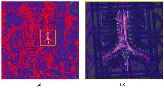
Figure 5.
IPSI network. All images shown with azimuth-slant range coordinates. Red points represent the PSCs, blue and white arcs represent the Delaunay triangulation network of PSCs before and after constraint that temporal coherence is above 0.6, and the green pentagram represents the starting point for SPU. (a) The whole study area; (b) T3 E area.
The initial offset of seasonal motion parameters in the proposed model is estimated by modeling the fitting curve of temperature listed in Table 1, as shown in Figure 6a. The blue asterisk represents the monthly average temperature of Beijing, in the years of 2012–2016. Thus, the initial offset is obtained by fitting the temperatures with seasonal deformation model (Equation (15)). After removing long arcs exceeding the threshold, the constrained Delaunay triangulation network of time/baseline plane for TPU is formed as shown in Figure 6b.
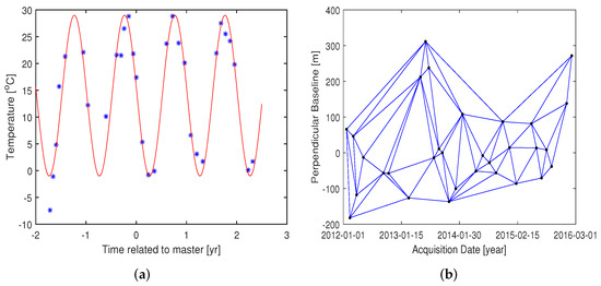
Figure 6.
SAR data representation. (a) Seasonal motion parameter fitting curves, the “−” before numbers in the picture is a minus sign; (b) the constrained Delaunay triangulation network in time/baseline plane for the TPU.
6.1. PU Comparison
First of all, we investigate the performance of the multi-component temporal coherence model from the conflict and effective edge number of 3D PU. The conflict and effective edges, used for effectively evaluating the 3D PU performance for real data [10,24,43], are defined as the edges whose unwrapped PGs’ absolute values are greater and not than , respectively. The 3D PU results based on linear and multi-component temporal coherence models are listed in Table 2, which presents the phase-consistency edges and ratio of the conflict edges over all arcs at four iterations in all interferograms. It is clearly shown from Table 2, that the statistical ratio based on both models are low for the high temporal coherence edges, and the ratio decreases as the temporal coherence intervals and iteration increase; while the number of phase-consistency edges is on the opposite. Moreover, more phase-consistency edges with higher temporal coherence are obtained based on the multi-component model than those based on the linear model at the fourth iteration. Although of the multi-component model is less than that of the linear model, of former is greater than the latter at the final iteration. On the whole, the 3D PU performance of the multi-component model is superior to that of the linear model.

Table 2.
The phase-consistency edges and ratio of conflict edges over all arcs at four iterations for all interferograms.
Secondly, the number of PSC arcs of the Delaunay triangulation network in azimuth/range plane before and after high temporal coherence constraint for the linear model and multicomponent model is compared in Figure 7. The same constraints, with temporal coherence greater than 0.65, 0.7, 0.75 and 0.75, respectively, for four iterations, are applied to optimize the path of SPU in both cases. It is observed that more PSCs arcs with low temporal coherence are removed for the case of linear model than that for multicomponent model. In addition, it can be seen from Figure 8 that the PU coverage based on multi-component temporal coherence model is better than that based on linear model, especially for the low-density PS area marked by yellow frame, which demonstrates that the multi-component model approximates the observed sample better than the linear model. In fact, the 2-D linear model is the special case of 3-D multicomponent model when estimated seasonal amplitude is zero, which indicates the generality of the multicomponent model.
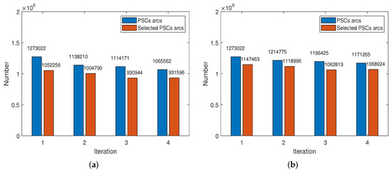
Figure 7.
Number of PSC arcs of the Delaunay triangulation network in azimuth/range plane before and after high temporal coherence constraint for linear model (a) and multicomponent model (b), respectively. The blue bars stand for the number of PSC arcs, while the brown bars stand for their selected ones with constraint.
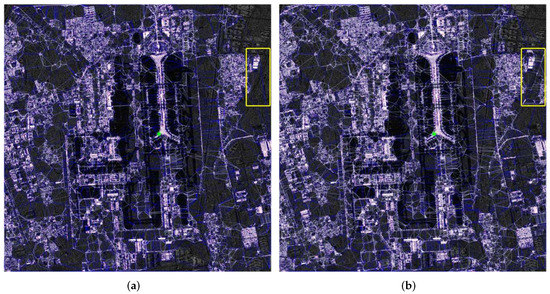
Figure 8.
The constrained Delaunay triangulation network in azimuth/range plane of PSCs at the final iteration for linear (a) and multicomponent (b) model. Red points represent the PSCs, blue and white arcs represent the Delaunay triangulation network of PSCs before and after high temporal coherence constraint.
Thirdly, the elapsed time of the 3D PU critical process is shown in Figure 9. The blue and brown bars represent the elapsed time in temporal coherence calculation and TPU + SPU, respectively. It is observed that under the same PSCs in the first iteration, although one additional dimension of variables and more PSC arcs need calculation, slightly inferior, 66.5 min, elapsed in the temporal coherence calculation procedure by the multi-component case, compared with 65 min for the linear case. It indicates the competitiveness of the multi-component model in elapsed time compared with the linear model.
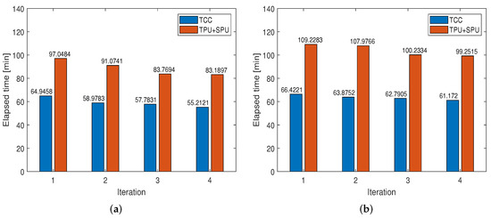
Figure 9.
Temporal coherence calculation (TCC) and PU elapsed time in each iteration; (a,b) list the elapsed time for linear and multi-component models, respectively.
6.2. PSCs Comparison
The number of PSCs with the coherence constraint based on both models is compared in Figure 10, where the blue bar represents the original number of PSCs, e.g., the original PSCs selected by for the first iteration and and and for the second, third and fourth iterations, while the brown bar represents the number after Delaunay triangulation network optimization. It is observed that from the first iteration, the same number of original PSCs, with 424,448, is obtained in both linear and multi-component cases. Moreover, it can be seen from the second bar to the fourth bar that more PSCs are retained in the multi-component case than in the linear case with the same selection principle. The final number of PS selected based on the multi-component model is 35,270 more than that based on the linear model, an increase by about . It demonstrates that there are more pixels with high temporal coherence in the multi-component case.
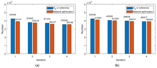
Figure 10.
PSCs Number before and after coherence threshold selection in each iteration. (a,b) list the number of PSCs for linear and multi-component models, respectively.
Secondly, according to the estimated time-series noise phase, the coherence and standard deviation (Std) of phase noise are calculated. As shown in Figure 11, the the same trend is observed from their histograms, that is, the coherence and Std of phase noise get better stepwise during four iterations, which indicates availability of the IPSI results based on both linear and multi-component models. Especially, the coherence and Std of phase noise based on the multi-component model is better than those based on the linear model.
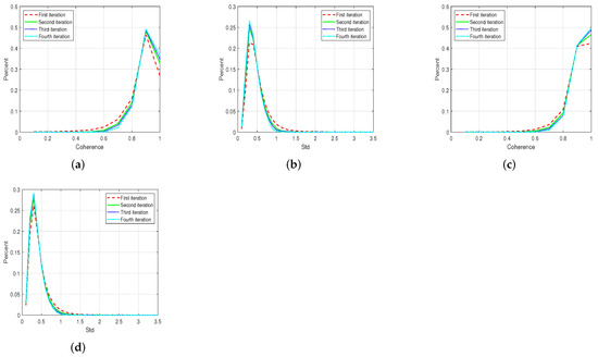
Figure 11.
The histograms of coherence and standard deviation of phase noise during four iterations. (a,b) are the histograms of coherence and standard deviation of phase noise based on the linear model, respectively, while (c,d) are based on the multi-component model.
6.3. Results Comparsion
The corrected DEM, deformation velocity and seasonal amplitude are shown in Figure 12, from which it can be seen that the new DEMs are significantly more accurate than the referred SRTM DEM (Figure 4c), in particular for the area of Terminal 3. The trend of corrected DEM is consistent with the TanDEM DEM of the Beijing Capital International Airport area. The consistent trend also applies to the deformation velocity by comparing with referred deformation velocity obtained by the StaMPS method from June 2003 to November 2013 [44]. The observed time overlapped about 2 years with the data set we used. However, there is some difference due to the difference of spatial resolution, especially for the DEM. Furthermore, more detail is presented by the estimated deformation velocities in both cases than the results obtained by the StaMPS method. Moreover, the same trend of topography, deformation velocity and seasonal amplitude can be observed from Figure 12 in both cases. From Figure 12c,f, we can find that most PS pixels have small seasonal displacement, which may be caused by seasonal change of underground water [41], and some buildings with thermal dilation [30,45,46].
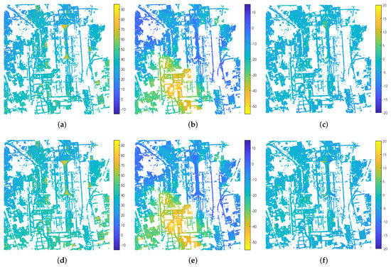
Figure 12.
IPSI final results. All results shown in azimuth-slant range coordination. The “−” before numbers in the picture is a minus sign. (a,d) are the corrected DEM [m] based on the linear and multi-component model, respectively, after adding residual topography back to the coarse DEM. (b,e) are deformation velocity [mm/yr] based on the linear and multi-component model, respectively. (c,f) are seasonal amplitude [mm] based on the linear and multi-component model, respectively.
Then, we investigate the results of common PS pixels in both cases. 353,845 common PS pixels, accounting for PS pixels in linear case, are plotted in Figure 13a. Their joint distributions of topography, deformation velocity and seasonal amplitude between both models are shown in Figure 13b–d, respectively. Given the results for common PS pixels, the evaluation result including bias, RMSE and , based on the multi-component model are listed in Table 3. It indicates the results for common PS pixels based on both models are close. The local statistics of cumulative deformation time series of one arbitrary local common pixel, located in subsidence area, are shown in Figure 13e,f, respectively. It is observed that the cumulative deformation time series based on both models are close. In fact, the RMSE of the cumulative deformation time series with respect to the modeled cumulative deformation is 2.99 mm. It demonstrates the effectiveness of the results based on the multi-component model.

Figure 13.
Comparisons of the common PS pixels’ results based on both model. (a) is for the common PS pixels selected. (b–d) are joint distribution of common PS pixels’ topography, deformation velocity and seasonal amplitude between both models. (e,f) represent statistics of the local 49 PS points’ cumulative deformation time series in case of linear and multi-component models for the PS pixels marked out by white circle in (a), and the blue dotted line stands for the mean modeled cumulative deformation [mm].

Table 3.
Evaluation results of the multi-component temporal coherence model.
Certainly, there is some difference due to the more PS results in multi-component case. Figure 14a shows the extra 36,607 pixels of the multi-component case. An arbitrary pixel, marked with green cross in Figure 14a, is chosen to confirm effectiveness of extra seasonal amplitude estimated in the multi-component case. As shown in Figure 14b,c, the distribution of residual deformation after subtracting the linear component is highly related to that of air temperature. The correlation coefficient is 0.9 by fitting the scatter diagram of temperature and residual deformation, which indicates the effectiveness of the multi-component model used for retrieving seasonal deformation. The results of local region for both cases, marked with yellow frame in Figure 14a, are magnified for comparison. In Figure 15, the red line above shows the local results based on linear model, while the below one shows the other case. It can be seen that the local results based on the multi-component model covers the objects better than the linear model. It is obvious that the lounge bridges of the T3 C building are clearly reconstructed by PS points. Quantitatively, the former covers 20,063 pixels, which is 13.3% more than the latter.
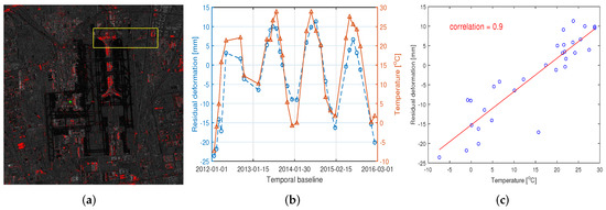
Figure 14.
Analysis of extra PS pixels the multi-component case more than the linear case. The “−” before numbers in the picture is a minus sign. (a) The extra PS pixels the multi-component case more than the linear case. (b) The distributions of residual deformation subtracting the linear component and air temperature. (c) Scatter plot and regression analysis of residual deformation and air temperature.

Figure 15.
Local results comparison for both models. The results above and below the red line based on linear and multi-component models, respectively. All images shown in azimuth-slant range coordination. (a) The corrected DEM [m]. (b) The LOS deformation velocity [mm/yr]. (c) The seasonal amplitude [mm].
Last but not least, as shown in Figure 16, the two models are compared in terms of uncertainties of residual topography, deformation velocity and seasonal amplitude. It is observed from their histograms that the uncertainties of residual topography, deformation velocity and seasonal amplitude in the multi-component case are better than those in the linear case. In detail, PS pixels with 0.5 m, 0.2 mm/yr and 0.2 mm estimation uncertainty in residual topography, deformation velocity and seasonal amplitude, respectively, account for 90.0%, 96.5% and 72.2% in the multi-component case, while they are, respectively, 85.1%, 94.8% and 61.5% in the linear case. As shown in the bottom row of Figure 16 for the uncertainties based on the multi-component model minus those based on the linear model, the result based on the multi-component model is better. In fact, when the coherence is above 0.65, the worst uncertainties from the multi-component model in residual topography, deformation velocity and seasonal amplitude estimation are 2.15 m, 0.59 mm/yr and 0.99 mm, respectively.
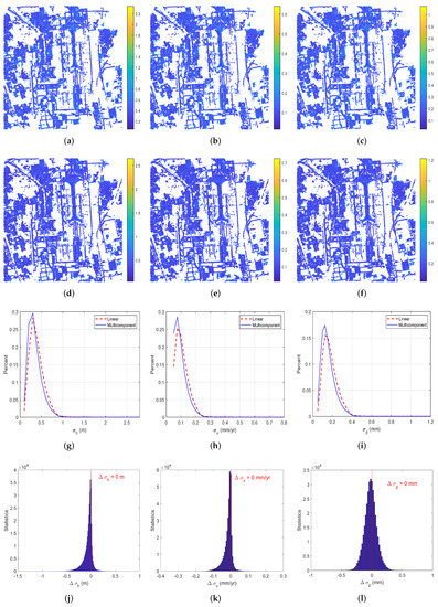
Figure 16.
Uncertainties evaluation of the results based on linear (top row) and multi-component (second row) models and their histograms (third row) and differential results of common pixels (last row). (a–f) represent the uncertainties of residual topography [m], deformation velocity [mm/yr] and seasonal amplitude [mm], respectively. (g–i) are the histograms of residual topography, deformation velocity and seasonal amplitude based on both models. (j–l) are the uncertainties based on the multi-component model minus those based on the linear model in terms of residual topography, deformation velocity and seasonal amplitude.The first, second and third columns represent the uncertainty of residual topography [m], deformation velocity [mm/yr] and seasonal amplitude [mm], respectively.
7. Conclusions
In this work, a multi-component temporal coherence model, which considers more components than the conventional linear model, has been developed for 3-D PU in TS-InSAR of seasonal deformation areas, and an uncertainty evaluation bound is derived for measuring the accuracy of residual topography, deformation velocity and seasonal amplitude. The multi-component temporal coherence model is applied to the IPSI, and its performance is demonstrated using a set of TSX/TDX data. In terms of PU evaluation, PS selection and final estimation results, the performance based on the multi-component model is better than the linear model given the same number of iterations and procedure. Compared with the 2-D linear model, it is found that the number of PS pixels selected with the same coherence threshold is increased by about 10%, 14.7% more arcs of PS pixels with high temporal coherence are used for 3D PU, and more PS pixels are of low uncertainty in residual topography, deformation velocity and seasonal amplitude estimation. Moreover, a competitive computing speed is obtained based on the multi-component model.
Author Contributions
Conceptualization, L.J. and B.Y.; formal analysis, B.Y. and H.X.; funding acquisition, L.J. and H.W.; investigation, L.J. and H.W.; methodology, H.X. and B.Y.; resources, H.X. and L.J.; supervision, L.J., H.X., Z.Z. and R.H.; validation, B.Y. and Z.Z.; writing—original draft, B.Y. and W.L. All authors have read and agreed to the published version of the manuscript.
Funding
This work was funded in part by the Key Research Program of the Chinese Academy of Sciences under Grant KFZD-SW-428, in part by the National Key R & D Program of China (2017YFA0603103), in part by the National Natural Science Foundation of China (41974009), and in part by the Key Research Program of Frontier Sciences, Chinese Academy of Sciences (QYZDB-SSW-DQC027, QYZDJ-SSW-DQC042).
Institutional Review Board Statement
Not applicable.
Informed Consent Statement
Not applicable.
Data Availability Statement
Not applicable.
Acknowledgments
We will thank for National Aeronautics and Space Administration (NASA) for making SRTM DEM data available.
Conflicts of Interest
The authors declare no conflict of interest.
References
- Zhu, X.; Wang, Y.; Montazeri, S.; Ge, N. A review of ten-year advances of multi-baseline SAR interferometry using TerraSAR-X data. Remote Sens. 2018, 10, 1374. [Google Scholar] [CrossRef] [Green Version]
- Ferretti, A.; Prati, C.; Rocca, F. Nonlinear subsidence rate estimation using permanent scatterers in differential SAR interferometry. IEEE Trans. Geosci. Remote Sens. 2000, 38, 2202–2212. [Google Scholar] [CrossRef] [Green Version]
- Ferretti, A.; Prati, C.; Rocca, F. Permanent scatterers in SAR interferometry. IEEE Trans. Geosci. Remote Sens. 2001, 39, 8–20. [Google Scholar] [CrossRef]
- Kampes, B. Displacement Parameter Estimation Using Permanent Scatterer Interferometry. Ph.D. Thesis, Delft University of Technology, Dutch, The Netherlands, 2005. [Google Scholar]
- Hooper, A.; Bekaert, D.; Spaans, K.; Arıkan, M. Recent advances in SAR interferometry time series analysis for measuring crustal deformation. Tectonophysics 2012, 514, 1–13. [Google Scholar] [CrossRef]
- Hooper, A.; Segall, P.; Zebker, H. Persistent scatterer interferometric synthetic aperture radar for crustal deformation analysis, with application to Volcán Alcedo, Galápagos. J. Geophys. Res. Solid Earth 2007, 112, 1–21. [Google Scholar] [CrossRef] [Green Version]
- Foroughnia, F.; Nemati, S.; Maghsoudi, Y.; Perissin, D. An iterative PS-InSAR method for the analysis of large spatio-temporal baseline data stacks for land subsidence estimation. Int. J. Appl. Earth Obs. Geoinf. 2019, 74, 248–258. [Google Scholar] [CrossRef]
- Fornaro, G.; Serafino, F. Imaging of single and double scatterers in urban areas via SAR tomography. IEEE Trans. Geosci. Remote Sens. 2006, 44, 3497–3505. [Google Scholar] [CrossRef]
- Yu, H.; Lan, Y.; Yuan, Z.; Xu, J.; Lee, H. Phase unwrapping in InSAR: A review. IEEE Geosci. Remote Sens. Mag. 2019, 7, 40–58. [Google Scholar] [CrossRef]
- Li, R.; Lv, X.; Yuan, J.; Yao, J. A triangle-oriented Spatial–Temporal phase unwrapping algorithm based on irrotational constraints for time-series InSAR. IEEE Trans. Geosci. Remote Sens. 2019, 57, 10263–10275. [Google Scholar] [CrossRef]
- Crosetto, M.; Monserrat, O.; Cuevas-González, M.; Devanthéry, N.; Crippa, B. Persistent scatterer interferometry: A review. ISPRS J. Photogramm. Remote Sens. 2016, 115, 78–89. [Google Scholar] [CrossRef] [Green Version]
- Fornaro, G.; Pauciullo, A.; Reale, D. A null-space method for the phase unwrapping of multitemporal SAR interferometric stacks. IEEE Trans. Geosci. Remote Sens. 2011, 49, 2323–2334. [Google Scholar] [CrossRef]
- Ghiglia, D.; Ghiglia, D.; Pritt, M.; Pritt, M. Two-Dimensional Phase Unwrapping: Theory, Algorithms, and Software; Living Away from Home: Studies; Wiley: New York, NY, USA, 1998. [Google Scholar]
- Yu, H.; Li, Z.; Bao, Z. Residues cluster-based segmentation and outlier-detection method for large-scale phase unwrapping. IEEE Trans. Image Process. 2011, 20, 2865–2875. [Google Scholar] [PubMed]
- Costantini, M.; Rosen, P.A. A generalized phase unwrapping approach for sparse data. In Proceedings of the IEEE 1999 International Geoscience and Remote Sensing Symposium—IGARSS’99 (Cat. No. 99CH36293), Hamburg, Germany, 28 June–2 July 1999; IEEE: Hamburg, Germany, 1999; Volume 1, pp. 267–269. [Google Scholar]
- Hooper, A. A statistical-cost approach to unwrapping the phase of InSAR time series. In Proceedings of the International Workshop on ERS SAR Interferometry, Frascati, Italy, 30 November–4 December 2009; Volume 30. [Google Scholar]
- Chen, C.W.; Zebker, H.A. Two-dimensional phase unwrapping with use of statistical models for cost functions in nonlinear optimization. JOSA A 2001, 18, 338–351. [Google Scholar] [CrossRef] [Green Version]
- Goldstein, R.M.; Zebker, H.A.; Werner, C.L. Satellite radar interferometry: Two-dimensional phase unwrapping. Radio Sci. 1988, 23, 713–720. [Google Scholar] [CrossRef] [Green Version]
- Costantini, M. A novel phase unwrapping method based on network programming. IEEE Trans. Geosci. Remote Sens. 1998, 36, 813–821. [Google Scholar] [CrossRef]
- Spoorthi, G.; Gorthi, R.K.S.S.; Gorthi, S. Phasenet 2.0: Phase unwrapping of noisy data based on deep learning approach. IEEE Trans. Image Process. 2020, 29, 4862–4872. [Google Scholar] [CrossRef]
- Sica, F.; Calvanese, F.; Scarpa, G.; Rizzoli, P. A CNN-based coherence-driven approach for InSAR phase unwrapping. IEEE Geosci. Remote Sens. Lett. 2020, 19, 4003705. [Google Scholar] [CrossRef]
- Hooper, A.; Zebker, H.A. Phase unwrapping in three dimensions with application to InSAR time series. JOSA A 2007, 24, 2737–2747. [Google Scholar] [CrossRef] [Green Version]
- Shanker, A.P.; Zebker, H. Edgelist phase unwrapping algorithm for time series InSAR analysis. JOSA A 2010, 27, 605–612. [Google Scholar] [CrossRef]
- Costantini, M.; Malvarosa, F.; Minati, F. A general formulation for redundant integration of finite differences and phase unwrapping on a sparse multidimensional domain. IEEE Trans. Geosci. Remote Sens. 2011, 50, 758–768. [Google Scholar] [CrossRef]
- Liu, F.; Pan, B. A new 3-D minimum cost flow phase unwrapping algorithm based on closure phase. IEEE Trans. Geosci. Remote Sens. 2019, 58, 1857–1867. [Google Scholar] [CrossRef]
- Pepe, A.; Lanari, R. On the extension of the minimum cost flow algorithm for phase unwrapping of multitemporal differential SAR interferograms. IEEE Trans. Geosci. Remote Sens. 2006, 44, 2374–2383. [Google Scholar] [CrossRef]
- Pepe, A.; Euillades, L.D.; Manunta, M.; Lanari, R. New advances of the extended minimum cost flow phase unwrapping algorithm for SBAS-DInSAR analysis at full spatial resolution. IEEE Trans. Geosci. Remote Sens. 2011, 49, 4062–4079. [Google Scholar] [CrossRef]
- Cuenca, M.C.; Hooper, A.J.; Hanssen, R.F. A new method for temporal phase unwrapping of persistent scatterers InSAR time series. IEEE Trans. Geosci. Remote Sens. 2011, 49, 4606–4615. [Google Scholar] [CrossRef]
- Kampes, B.M.; Hanssen, R.F. Ambiguity resolution for permanent scatterer interferometry. IEEE Trans. Geosci. Remote Sens. 2004, 42, 2446–2453. [Google Scholar] [CrossRef] [Green Version]
- Zhu, X.X.; Bamler, R. Let us do the time warp: Multicomponent nonlinear motion estimation in differential SAR tomography. IEEE Geosci. Remote Sens. Lett. 2011, 8, 735–739. [Google Scholar] [CrossRef] [Green Version]
- Colesanti, C.; Ferretti, A.; Novali, F.; Prati, C.; Rocca, F. SAR monitoring of progressive and seasonal ground deformation using the permanent scatterers technique. IEEE Trans. Geosci. Remote Sens. 2003, 41, 1685–1701. [Google Scholar] [CrossRef] [Green Version]
- Kay, S.M. Fundamentals of Statistical Signal Processing: Estimation Theory; Prentice-Hall, Inc.: Upper Saddle River, NJ, USA, 1993. [Google Scholar]
- KAY, S.M. Fundamentals of Statistical Signal Processing; Prentice Hall: Upper Saddle River, NJ, USA, 1998. [Google Scholar]
- Zachariah, D.; Stoica, P. Cramér-rao bound analog of bayes’ rule [lecture notes]. IEEE Signal Process. Mag. 2015, 32, 164–168. [Google Scholar] [CrossRef]
- Prasad, R.; Murthy, C.R. Cramér–Rao-type bounds for sparse Bayesian learning. IEEE Trans. Signal Process. 2012, 61, 622–632. [Google Scholar] [CrossRef] [Green Version]
- Stoica, P.; Nehorai, A. MUSIC, maximum likelihood, and Cramer–Rao bound. IEEE Trans. Acoust. Speech Signal Process. 1989, 37, 720–741. [Google Scholar] [CrossRef]
- Sun, P.; Tang, J.; He, Q.; Tang, B.; Tang, X. Cramer–Rao bound of parameters estimation and coherence performance for next generation radar. IET Radar Sonar Navig. 2013, 7, 553–567. [Google Scholar] [CrossRef]
- Zhao, B.; Haldar, J.P.; Liao, C.; Ma, D.; Jiang, Y.; Griswold, M.A.; Setsompop, K.; Wald, L.L. Optimal experiment design for magnetic resonance fingerprinting: Cramer–Rao bound meets spin dynamics. IEEE Trans. Med. Imag. 2018, 38, 844–861. [Google Scholar] [CrossRef] [PubMed]
- Zhu, X.X.; Bamler, R. Super-resolution power and robustness of compressive sensing for spectral estimation with application to spaceborne tomographic SAR. IEEE Trans. Geosci. Remote Sens. 2011, 50, 247–258. [Google Scholar] [CrossRef]
- Yang, B.; Xu, H.; Liu, W.; You, Y.; Xie, X. Realistic lower bound on elevation estimation for tomographic SAR. IEEE J. Sel. Top. Appl. Earth Observ. Remote Sens. 2018, 11, 2429–2439. [Google Scholar] [CrossRef]
- Zhou, C.; Gong, H.; Zhang, Y.; Warner, T.A.; Wang, C. Spatiotemporal evolution of land subsidence in the Beijing plain 2003–2015 using persistent scatterer interferometry (PSI) with multi-source SAR data. Remote Sens. 2018, 10, 552. [Google Scholar] [CrossRef] [Green Version]
- Wang, C.G.; Wang, Z.Z.; Ke, C. Structure Design of Beijing Capital International Airport Terminal 3. Build. Struct. 2008, 38, 16–24. [Google Scholar]
- Li, S.; Xu, H.; Gao, S.; Li, C. A non-fuzzy interferometric phase estimation algorithm based on modified Fully Convolutional Network. Pattern Recognit. Lett. 2019, 128, 60–69. [Google Scholar] [CrossRef]
- Gao, M.; Gong, H.; Chen, B.; Zhou, C.; Chen, W.; Liang, Y.; Shi, M.; Si, Y. InSAR time-series investigation of long-term ground displacement at Beijing Capital International Airport, China. Tectonophysics 2016, 691, 271–281. [Google Scholar] [CrossRef]
- Ma, P.; Lin, H.; Lan, H.; Chen, F. Multi-dimensional SAR tomography for monitoring the deformation of newly built concrete buildings. ISPRS J. Photogramm. Remote Sens. 2015, 106, 118–128. [Google Scholar] [CrossRef]
- Ma, P.; Wang, W.; Zhang, B.; Wang, J.; Shi, G.; Huang, G.; Chen, F.; Jiang, L.; Lin, H. Remotely sensing large-and small-scale ground subsidence: A case study of the Guangdong–Hong Kong–Macao Greater Bay Area of China. Remote Sens. Environ. 2019, 232, 111282. [Google Scholar] [CrossRef]
Publisher’s Note: MDPI stays neutral with regard to jurisdictional claims in published maps and institutional affiliations. |
© 2022 by the authors. Licensee MDPI, Basel, Switzerland. This article is an open access article distributed under the terms and conditions of the Creative Commons Attribution (CC BY) license (https://creativecommons.org/licenses/by/4.0/).