Article

The Use of C-Band and X-Band SAR with Machine Learning for Detecting Small-Scale Mining

by
Gabrielle Janse van Rensburg
1,2,* and
Jaco Kemp
2
1
Council for Geoscience, Pretoria 0184, South Africa
2
Department of Geography and Environmental Studies, Stellenbosch University, Stellenbosch 7602, South Africa
*
Author to whom correspondence should be addressed.
Remote Sens. 2022, 14(4), 977; https://doi.org/10.3390/rs14040977
Submission received: 4 November 2021 / Revised: 1 December 2021 / Accepted: 6 December 2021 / Published: 17 February 2022

Abstract

:
Illicit small-scale mining occurs in many tropical regions and is both environmentally and socially hazardous. The aim of this study was to determine whether the classification of Synthetic Aperture Radar (SAR) imagery could detect and map small-scale mining in Ghana by analyzing multi-temporal filtering applied to three SAR datasets and testing five machine-learning classifiers. Using an object-based image analysis approach, we were successful in classifying water bodies associated with small-scale mining. The multi-temporally filtered Sentinel-1 dataset was the most reliable, with kappa coefficients at 0.65 and 0.82 for the multi-class classification scheme and binary-water classification scheme, respectively. The single-date Sentinel-1 dataset has the highest overall accuracy, at 90.93% for the binary water classification scheme. The KompSAT-5 dataset achieved the lowest accuracy at an overall accuracy of 80.61% and a kappa coefficient of 0.61 for a binary-water classification scheme. The experimental results demonstrated that it is possible to classify water as a proxy to identify illegal mining activities and that SAR is a potentially accurate and reliable solution for the detection of SSM in tropical regions such as Ghana. Therefore, using SAR can assist local governments in regulating small-scale mining activities by providing specific spatial information on the whereabouts of small-scale mining locations.

1. Introduction

Small-scale mining (SSM) has devastating impacts on the natural environment when not regulated properly, and many small-scale mining operations are operated illegally. SSM is a low-cost, labor-intensive method of mining [1] in areas where gold is easily accessible, such as on the river banks where alluvial gold deposits can be found. Land degradation is a consequence of such mining activities and remains an important global issue, as the global demand for precious minerals will continue to increase [2]. Around two-thirds of the total supply of these minerals comes from countries in South America, South Asia, and Sub-Saharan Africa [3].
In Ghana, “galamsey” is a term commonly used to describe illegal mining activity in Ghana. Mantey et al. [4] and Owusu-Nimo et al. [5] suggest that galamsey operations are an illegal or unregulated form of SSM and processing of gold that lies at or below soil and water surfaces in Ghana. Galamsey operations have historically only been associated with simple tools and manual labor [6,7] but the use of mechanized equipment like excavators has recently also come into play [4,8], most probably due to the influx of foreign nationals who changed the operational dynamics of galamsey operations [4]. The precious minerals are gathered discreetly and sold in contravention of state laws [4,9]. Galamseyers also do not pay tax, many mines are in delicate or prohibited areas, and often, human safety is put at risk [5,10,11,12].
Galamsey operations tend to leave behind many wastelands in the form of pits flooded with water, deforested lands, and polluted water bodies [5,13] that are hazardous to the local people, livestock and wildlife. Accessing SSM sites is difficult due to their remote locations and is extremely dangerous [5,14]. Remote sensing provides a way to monitor such remote locations on a regular basis, but the use of optical imagery is restricted because of the tropical climate of Southern Ghana. Snapir et al. [
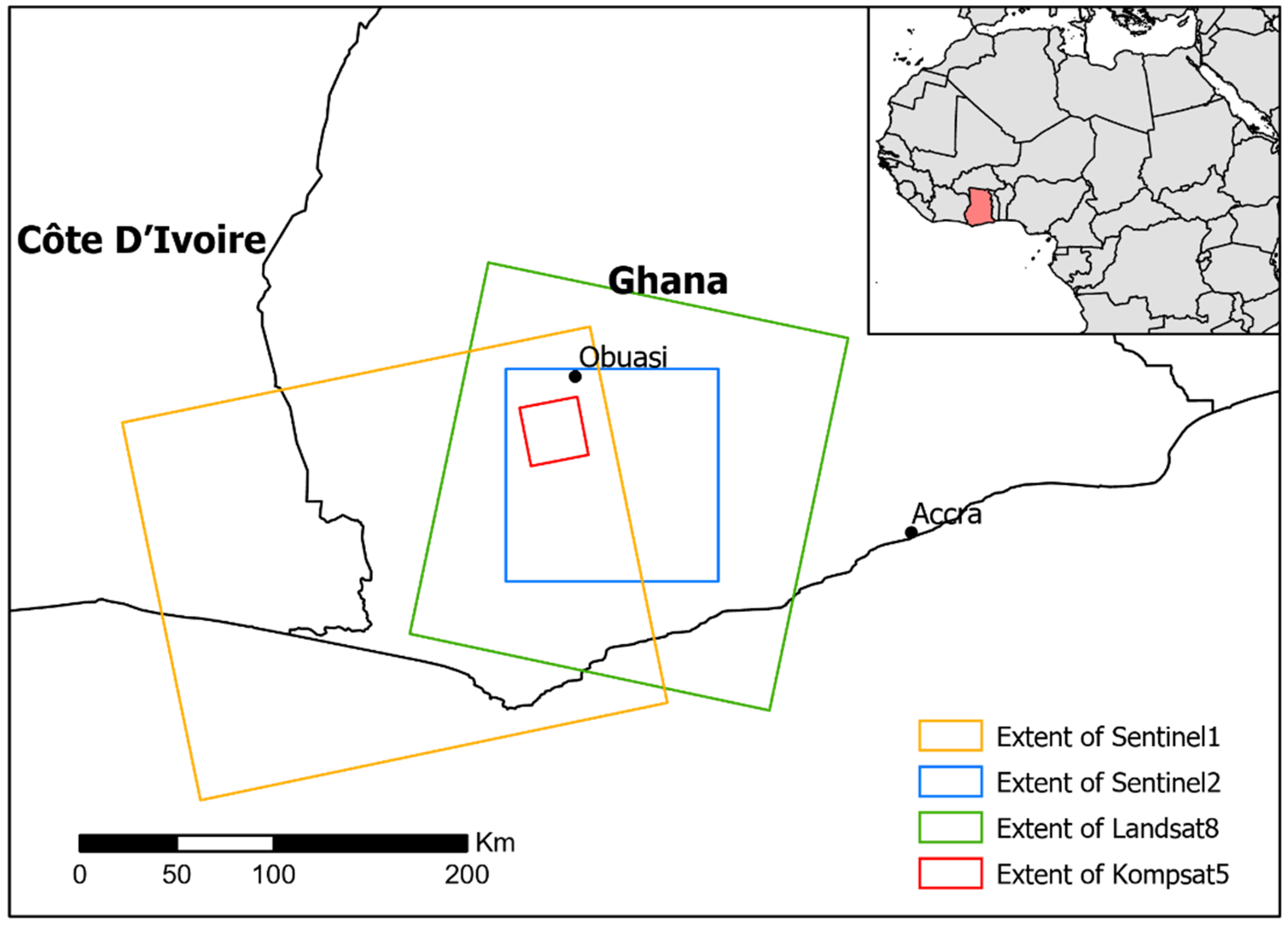
15], who attempted to map the expanding areas of galamsey, had difficulty in obtaining cloud-free imagery to evaluate change detection. They only found one cloud-free Landsat-8 image and were unable to find suitable Landsat images for multi-temporal compositing for their study in Ghana. The effective monitoring of such large-scale unregulated mining activity requires a continuous supply of image data that is available year-round, as well as night and day.
Synthetic Aperture Radar (SAR) imagery presents a solution due to the active nature of SAR sensors, which emit microwaves that can penetrate through clouds and also function during the nighttime [16,17,18]. Except for one recently published study by [19], SAR has not yet been applied to the mapping and monitoring of SSM in Ghana. SAR can provide valuable insights into the specific locations of SSM and the growth rate of galamsey over time [20]. Questions such as, “In which seasons are SSM most active?” have not yet been answered. Having an uninterrupted supply of usable, easily obtainable imagery, as provided by Sentinel-1, could provide governments with strategic information to improve regulation efforts to address the issues associated with SSM [4,5]. Globally, SAR has been used extensively for different applications requiring an active sensing system that is not affected by cloud cover or the time of day, such as the monitoring of ships, wetlands, floods and deforestation [21,22,23]. SAR is also used for the monitoring of crops such as sugarcane [24], or the mapping of the geomorphology of coastlines [25] using its scattering properties. Further examples of the application of SAR can be seen in [26,27,28].
Remote sensing has been widely used for the application of land cover classification [29] as a method for mapping and monitoring land use [30]. Land cover mapping is essential for the estimation of land cover change because land cover change is directly related to human and natural health and growth [30,31,32]. Typical applications of land cover classification are in the estimation of deforestation, for analyzing the extent of flood events, and determining areas for biodiversity conservation [30,33,34,35]. Additionally, it can be used for monitoring illegal logging and mining activities in remote locations [5,14,36].
Land cover mapping using remote sensing is driven by the need for knowledge of the spatial distribution of land use and land cover (LULC) [27]. Remote sensing data has become easily accessible, and the advancement of computers and algorithms has caused immense growth in the field of land cover classification [37]. Classified images are then used to assist in policymaking and decision-making on the effects of urbanization and industrial development, illegal activities, protecting important natural areas, human settlement planning, food security and more [31,38,39,40], especially in remote areas where data is scarce. Classification is, therefore, a potential approach to mapping SSM in remote areas.
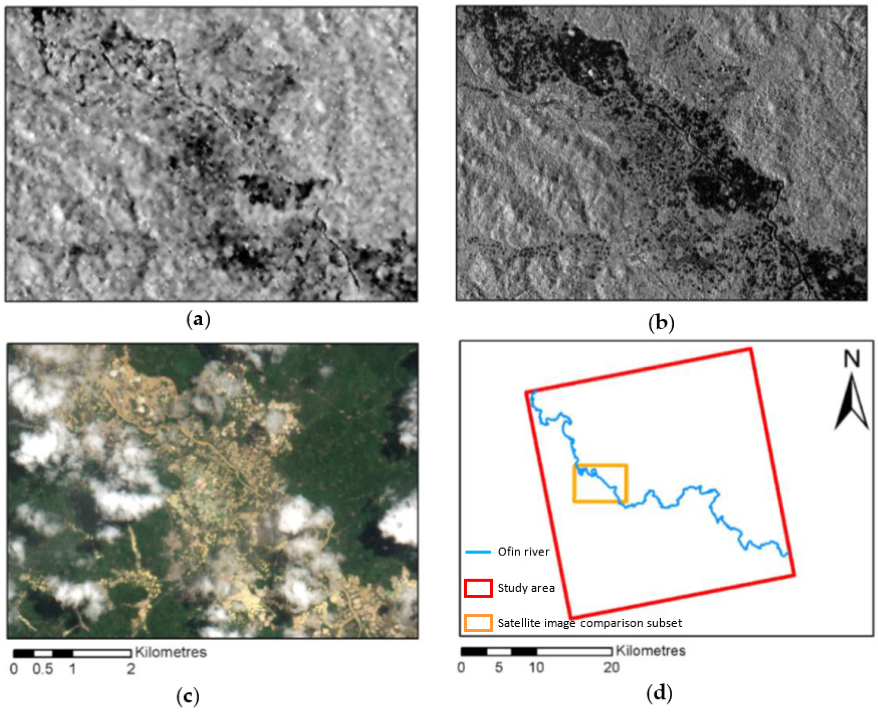
SSM sites around rivers typically comprise extensive, intermixed areas of bare soil and water pools resulting from the mining process [14]. A typical pool of water after the mining process has begun is about 20 m in diameter, which challenges the spatial resolution limits of Sentinel-1. However, using multi-date imagery often produces more accurate results than single-date imagery [14]. The application of multi-temporal filtering of SAR for monitoring SSM has not yet been tested. SAR flood monitoring also provides insight into mapping the water pools of the alluvial SSM sites, by using change detection (e.g., [41,42]). Since around the year 2000, machine learning classification algorithms such as random forests have been tested and found to give reliable classification results on SAR imagery [41,43,44,45]. Different machine learning classifiers have not yet been compared for the classification of SSM with SAR imagery. Classifying SAR imagery is more challenging than classifying optical imagery because ground features are harder to distinguish with the human eye than those that can be seen in optical imagery. Knowing which classifier produces the most accurate and reliable results is important for an effective monitoring system.
Most of the literature with regards to illegal mining or small-scale mining globally is about policymaking, such as the studies by [1,6,46,47,48,49,50,51,52], or the environmental impacts or health assessments that involve manual sampling methods, such as the studies by [53,54,55,56,57,58]. Only a few examples exist of where remote sensing is used to map or monitor SSM and these include [14,15,36,59], who used optical imagery.
Almeida-Filho and Shimabukuro [60] have published the only study so far using the backscatter values of SAR to map the degeneration caused by SSM. The aim of their study was to investigate the possibility of using SAR to detect degradation areas caused by independent gold miners, “garimpeiros”, in the Amazon because of the regular cloud cover in the region. Almeida-Filho and Shimabukuro [60] used three 18-m resolution, L-band, HH polarization Japanese Earth Resource Satellite-1 (JERS-1) images from the years 1993 (dry season), 1994 (rainy season), and 1996 (rainy season). Speckle filtering was applied with a 7 × 7 window kernel and the images were resampled to 30 m resolution to match the resolution of Landsat TM, acquired in 1994, which was used as the reference image. Their study area was the Tepequém plateau, situated in northern Brazil, which consisted of savannah grass that was surrounded by tropical rain forest. They found that the low grassland vegetation produced subtle tonal contrasts in the SAR imagery compared to the high contrast produced by deforestation in studies performed in the forested areas, e.g., [61,62,63]. The similar backscatter responses between the eroded areas and the savannah grass made identification of the degraded areas from gold-mining activities unidentifiable when using a single-date JERS-1 SAR image. Their change detection normalized difference index (NDI) technique showed that the land cover change was detectable with the low tonal contrast of the grasslands. Due to the lack of a reliable classifier for SAR imagery, the authors of [60] were unable to produce a thematic map of the degradation areas found in their 1993–1994 NDI image.
From the study by Almeida-Filho and Shimabukuro [60], it is clear that SAR has the potential to detect SSM. Their challenge of detecting the degradation areas in single-date imagery can be tested over forested areas where gold mining takes place, such as in Ghana. The recent publication of research by [19] proved that SSM in Ghana can be detected with SAR. They used Sentinel-1 time series data and compared the mean, minimum, and maximum backscatter difference images of both polarizations. They found that the minimum backscatter images were the most sensitive to detecting changes caused by mining-induced land cover changes in Ghana and that a threshold value of +1.65 dB was suitable to classify this change. It is, however, uncertain what the impact of multi-temporal filtering of a time series of Sentinel-1 imagery would have on SSM detection accuracies. The use of a wider variety of machine learning algorithms, especially applied to different SAR wavelengths and features, has not been sufficiently investigated.
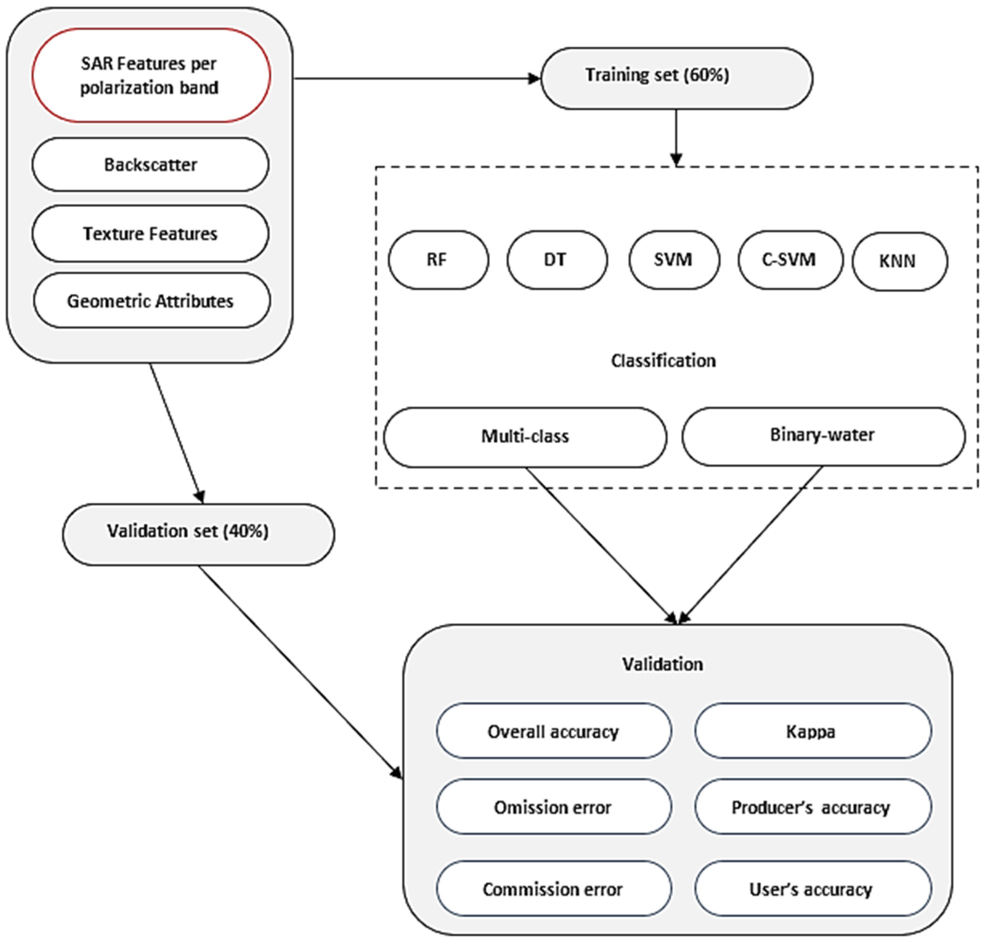
In this study, we evaluated how different SAR sensors compare regarding the mapping of SSM when applying classification. We tested how single-product speckle-filtered SAR performed, compared with multi-temporal filtered SAR, when applying classification, and which classification algorithm is best suited for the mapping of SSM with SAR imagery.

2. Materials and Methods

2.1. Study Area

The study area is located in Southern Ghana, which includes the Ofin River near the mining town of Obuasi (Figure 1). The study area is rural and dominated by forests. Southern Ghana has a tropical climate with daytime temperatures ranging between 25 and 35 degrees Celsius [64]; the most rainfall occurs between July and September and the average annual rainfall is 736.6 mm [65]. The absence of large buildings in the scattered rural settlements is beneficial for applying remote sensing with SAR since the buildings will not interfere with the radar signal. Buildings produce a double-bounce effect that reflects the microwave energy back to the sensor very strongly.

2.2. Data Collection

The data used in this study consists of multiple Sentinel-1 images and one KompSAT-5 image. Sentinel-1 is freely available through the Copernicus Open Access Hub and the KompSAT-5 image was sponsored by SI-Imaging. For ground truth validation, open-access Sentinel-2 imagery was used. The Sentinel-1 imagery is C-band (5.405 GHz) SAR backscatter with incidence angles ranging from 32.9° to 43.1° and the spatial resolution is 20 m. The Sentinel-1 imagery was accessed as interferometric wide-swath (IW) single-look complex (SLC) products from the Copernicus Open Access Hub. IW offers dual-polarization capability, with vertical transmit–horizontal receive (VH) and vertical transmit–vertical receive (VV). The range of dates for the Sentinel-1 imagery is from August 2017 to August 2018 and one image was selected for each month. While all 13 images were used for the multi-temporal filtering process, classification was only performed on the 12 August 2018 image.
The KompSAT-5 (Korea multi-purpose satellite) X-band (9.66 GHz) image used in this experiment was provided by SI-Imaging Services. KompSAT-5′s enhanced standard (ES Standard) mode is similar to Sentinel-1′s IW mode, with single-polarization VH. The incidence angle ranges from 28.8° to 55°, the spatial resolution is 3 m, and it covers a swath of 30 km (SI-Imaging Services 2019). The date of acquisition was 12 July 2018.
Sentinel-2 optical imagery was used as the ground truth dataset for training and validation purposes. The aim was to retrieve an image with the least amount of cloud cover, closest to the date of the single-date SAR imagery (July/August 2018). Sentinel-2 imagery is also freely available through the Copernicus Open Access Hub. Level-1C imagery was downloaded and only the true color band combination (RGB 4-3-2) at 10 m spatial resolution was used. Figure 2 displays an example of each of the Sentinel-1 and the KompSAT-5 imagery over an area where abundant SSM takes place, surrounding the Ofin River. The ground truth Sentinel-2 image is also shown over the same area segment.
The Sentinel-1 toolbox, available in SNAP, was used for the pre-processing of both the Sentinel-1 and KompSAT-5 datasets. Pre-processing involved the radiometric calibration, geocoding, and terrain correction of all images. The single-date images were speckle-filtered using the Lee Sigma (7 × 7) filter, and the multi-temporal Sentinel-1 dataset underwent image co-registration and multi-temporal filtering, also with the Lee Sigma (7 × 7) filter. These filtered datasets will be referred to as S1 and S1-MT, respectively, in this article. All filtered images were converted to decibel format. Additional textural features were derived from each dataset using PCI Geomatica’s TEX algorithm to calculate the grey-level co-occurrence matrix (GLCM) for each polarization band. The following eight texture measures were calculated: homogeneity, contrast, dissimilarity, mean, variance, entropy, angular second moment (ASM), and correlation.

2.3. Methodology

The research design is illustrated in Figure 3. First, the SAR features were extracted per object after image segmentation was applied. Then, samples were collected for input to the training and testing datasets for the machine learning classifiers. Next, the classifier was run on each dataset. Lastly, validation statistics were performed to analyze the accuracy and reliability of each classifier or dataset.

2.3.1. Sample Collection

Samples were selected to use as input for the training and testing of the machine learning classifiers. Samples were collected on the Sentinel-1 multi-temporally filtered image (S1-MT) by selecting objects from the segmentation results and visually confirming on the Sentinel-2 image to which class the object belongs. Two classification scheme designs were tested. The first classification scheme was a binary-water classification scheme consisting of two classes: water and non-water. Binary classification schemes are simple and highly accurate where the classification scheme merely consists of, for example, water and non-water. After several studies attempted to take advantage of the very low backscatter received from water bodies [66,67,68,69] it has been established that when mapping large water bodies, the simple single-threshold method did not produce good results [70] because of the variability of the environment, such as wind-roughening and satellite parameters [71,72]. Spatial and temporal variety in backscatter also occurred in permanent water bodies in the study by [73]. The second classification scheme was a multi-class classification scheme that consisted of the following classes: water, bare ground, vegetation and built-up area. This was performed to compare binary classification results to a more generic classification scheme approach that is popularly used for land cover classification applications (e.g., [74,75]). Both classification schemes are of interest for this study, to compare the accuracy and robustness of the classification algorithms. The descriptions of each class are listed in Table 1. The number of samples collected was 197 per class. Thus, the multi-class classification database consisted of 788 samples, and the binary-water classification database comprised 394 samples.

2.3.2. Image Classification Part 1: SAR Dataset Comparison

The input SAR datasets with all the calculated features are summarized in Table 2 where the texture features include homogeneity, contrast, dissimilarity, mean, variance, entropy, ASM, and correlation, and the geometric attributes are count, rectangularity, length/width, compactness, and roundness. The SAR datasets are the single-date Sentinel-1 (S1), single-date KompSAT-5 (K5), and multi-temporally filtered Sentinel-1 (S1-MT) datasets that consist of the backscatter values, texture features and geometric attributes for each polarization band.
The SAR datasets were classified using the random forest machine-learning algorithm. Random forest (RF) is a classifier that fits a number of decision tree classifiers on various subsamples of the dataset. RF then uses averaging to improve the predictive accuracy and to control overfitting. Breiman (2001) defines RF as a “combination of tree predictors such that each tree depends on the values of a random vector sampled independently and with the same distribution for all trees in the forest” [76]. RF selects the best solution from all the predictive sets by means of a voting parameter and RF stores the significance of the input features [26]. The classifier was run 1000 times using the Python-based scikit-learn libraries, where the dataset was split on 40% for the test size and the samples were selected according to a stratified random approach.

2.3.3. Image Classification Part 2: Machine Learning Classification Comparison

The five most commonly used machine learning classifiers employed in the classification of remote sensing datasets are: k-nearest neighbor (KNN), decision trees (DT), random forest (RF), the support vector machine (SVM), and kernel support vector machine (C-SVM) [45]. The popularity of these algorithms for remote sensing applications is because of their ease of use, computational efficiency and adaptability [77]. Each classification algorithm uses a different mathematical model as an approach to pattern recognition and the prediction of classes.
Decision trees represent a supervised machine learning method that uses a tree-like model based on conditional control statements. This non-parametric method is used for classification and regression analysis. The DT algorithm creates a model that predicts a target value through learned decision rules that are inferred from the data input features [78].
Neighbors-based classification, such as k-nearest neighbor, is a type of instance-based learning where new problem instances are compared with instances seen in training. The algorithm does not attempt to construct an internal model but only stores instances of the training data in the memory [79]. KNN performs classification based on approximate locality from the major votes of the nearest neighbor of each point using, e.g., the Euclidean distance between points [78].
Support vector machines are used for classification and regression analysis by building an internal model that works well for non-linear datasets [80,81]. The algorithm takes input vectors and maps them non-linearly onto a high-dimension feature space, to maximize the width of the gaps between categories using a hyperplane [80]. When a hyperplane cannot separate the two categories while maximizing the margin, C-SVM is used, where C is the regularization parameter that has an inverse relationship with the margin [82]. SVM utilizes kernel functions that map the input data to higher dimensions to achieve the optimal hyperplane for maximum separation between classes [80]. The types of kernels used by SVM are linear, polynomial, sigmoid and radial base function (RBF), where the RBF-kernel is commonly used in many applications [83]. SVM is a highly accurate classifier compared to classifiers such as decision trees [84].
Image classification was conducted with the same methodology as was used for the SAR dataset comparison, but it was only performed on the S1-MT dataset. Each classifier was run separately for both classification schemes and the test set size remained at 40%. The dataset was split with each run of the classifier and the classifier ran 1000 times. All classifiers were trained using the same set of input features of S1-multi as in the SAR dataset comparison, which included intensity bands, texture layers, and geometric features. The classifiers tested were RF, DT, SVM (with linear kernel function), C-SVM (with RBF kernel function), and KNN.

2.3.4. Accuracy Assessment

Confusion matrices were created for each classifier and classification scheme, to measure the relative performance of each classifier. The average of each position in the confusion matrix was calculated from the 1000 iterations of the classifier, to create a derived confusion matrix for each classification scheme. Error metrics like producer’s and user’s accuracies, overall accuracy and kappa coefficient were derived from the matrix. The kappa coefficient is an important metric often used in the accuracy assessment of classification results in remote sensing applications [85,86]. The kappa coefficient is not an index of accuracy, but is instead an indication of agreement beyond chance and has been criticized as unsuited for typical remote sensing applications [86]. Despite this criticism, the kappa coefficient was reported in this study for ease of comparison, since it has been used by many remote sensing studies for an accuracy assessment of the production of thematic maps (e.g., [45,85,87]).
The statistical significance was measured with the area under the curve (AUC) method that is based on probability assessment. The standard normal value (z), together with the confidence level, which was set at 95%, is then used to get the probability from the probability tables that can be found in the study by [88]. The higher the probability, the larger the area under the curve and, therefore, the more significant the result. The z-scores were calculated using the means and standard deviations of the overall accuracy results of each classifier on the multi-class classification scheme.

3. Results

3.1. SAR Datasets Comparison

The S1-MT dataset has the highest overall accuracy at 73.60% for the multi-class classification scheme and S1 has the highest overall accuracy at 90.93% for the binary water classification scheme (Figure 4). However, the S1-MT dataset has the highest kappa coefficients at 0.65 and 0.82 for the multi-class classification scheme and binary-water classification scheme, respectively. The K5 dataset yielded the lowest overall accuracy and kappa coefficients at 80.61 and 0.61, respectively, for both the multi-class classification scheme and the binary-water classification scheme.
Table 3 summarizes the producer’s and user’s accuracies for the “water” class with RF between the datasets. The S1-MT dataset PA is 2.28% and 20.76% higher, and the UA is 2.61% and 21.57% higher than S1 and K5, respectively, in terms of the “water” class of the multi-class classification scheme. The S1-MT dataset also outperformed the S1 and K5 datasets with the binary-water classification scheme at 1.58% and 11.05% higher PA, and 0.33% and 9.49% higher UA, for S1 and K5, respectively.
The average error of omission and commission values summarized in Table 4 confirms why the multi-class classification scheme performed poorly compared to the binary-water classification scheme. For the S1-MT dataset, 26.40% of reference sites were left out (omitted) and 26.26% of the objects were incorrectly classified (committed) for the multi-class classification scheme, compared to a 9.07% omission error and 9.00% commission error for the binary-water classification scheme. The individual confusion matrices for all three datasets and both classification schemes are listed in Appendix A.

3.2. Machine Learning Classifier Comparison

For the machine learning classifier comparison, RF outperformed all the classifiers, with an average overall accuracy of 73.60% and 90.04% for the multi-class classification scheme and binary-water classification scheme, respectively (Figure 5). The second-best performing classifier was C-SVM with an average overall accuracy of 70.15% and 89.17% for the multi-class classification scheme and binary-water classification scheme, respectively. SVM and C-SVM performed very similarly, and DT and KNN yielded the lowest overall accuracy and kappa coefficients. RF was significantly better than the other classifiers, according to the area under the curve method. Random forest showed the highest probability score at 0.87, whereas decision trees had the lowest probability score of 0.12. The probability results are displayed in Table 5.
Table 6 summarizes the producer’s and user’s accuracies of the “water” class classification on S1-MT of DT, RF, KNN, SVM, and C-SVM. RF had the highest PA and UA results, except in the case of the UA of the multi-class classification scheme that belongs to SVM. The RF classifier is 3.9% higher in PA than the second-best result of C-SVM for the multi-class classification scheme, and 10.85% higher in PA than DT, which gave the lowest result. For the binary water classification scheme, RF outperformed C-SVM by 1.67% in PA and DT, again, with the lowest result at 6.44% lower than the PA of RF. The UA in the multi-class classification scheme was the highest at 81.87% for SVM, 0.65% better than the UA of RF; the UA of SVM is also 10.95% higher than the UA of KNN, which gave the lowest result. The UA in the binary-water classification scheme was the highest for RF at 89.29%, with a 0.25% difference from SVM and 3.35% difference from KNN, again the lowest result.
Figure 6 visually shows the RF classification results on the multi-temporally filtered S1 dataset (S1-MT). Figure 6a shows the multi-class land cover classification map, where blue is water, green is vegetation, orange is bare ground and grey is built-up area. The image indicates that built-up areas and bare ground are incorrectly classified in the vegetation and river areas. The confusion matrix calculated confirms high errors of commission for bare ground and built-up area at 38.88% and 18.50%, respectively. The water-binary land cover classification map (Figure 6b) clearly shows the extent of water pools along the river, stretching into the vegetated areas. The reduction of classes from four to two led to more accurate results, albeit at the cost of class granularity.
For the SAR dataset comparison (image classification part 1) the multi-class classification scheme yielded unreliable results, whereas the average kappa coefficient for all datasets and classification algorithms was 0.54, as shown in Table 7. The binary-water classification scheme gave reliable results with an average kappa coefficient of 0.75. With the multi-class classification scheme, confusion between classes took place, as can be seen in Table 7, whereas the binary-water classification could clearly distinguish between the water objects and the non-water objects. The confusion matrices of all results are given in Appendix A Table A1, Table A2, Table A3, Table A4, Table A5, Table A6, Table A7, Table A8, Table A9, Table A10, Table A11, Table A12, Table A13 and Table A14.

4. Discussion

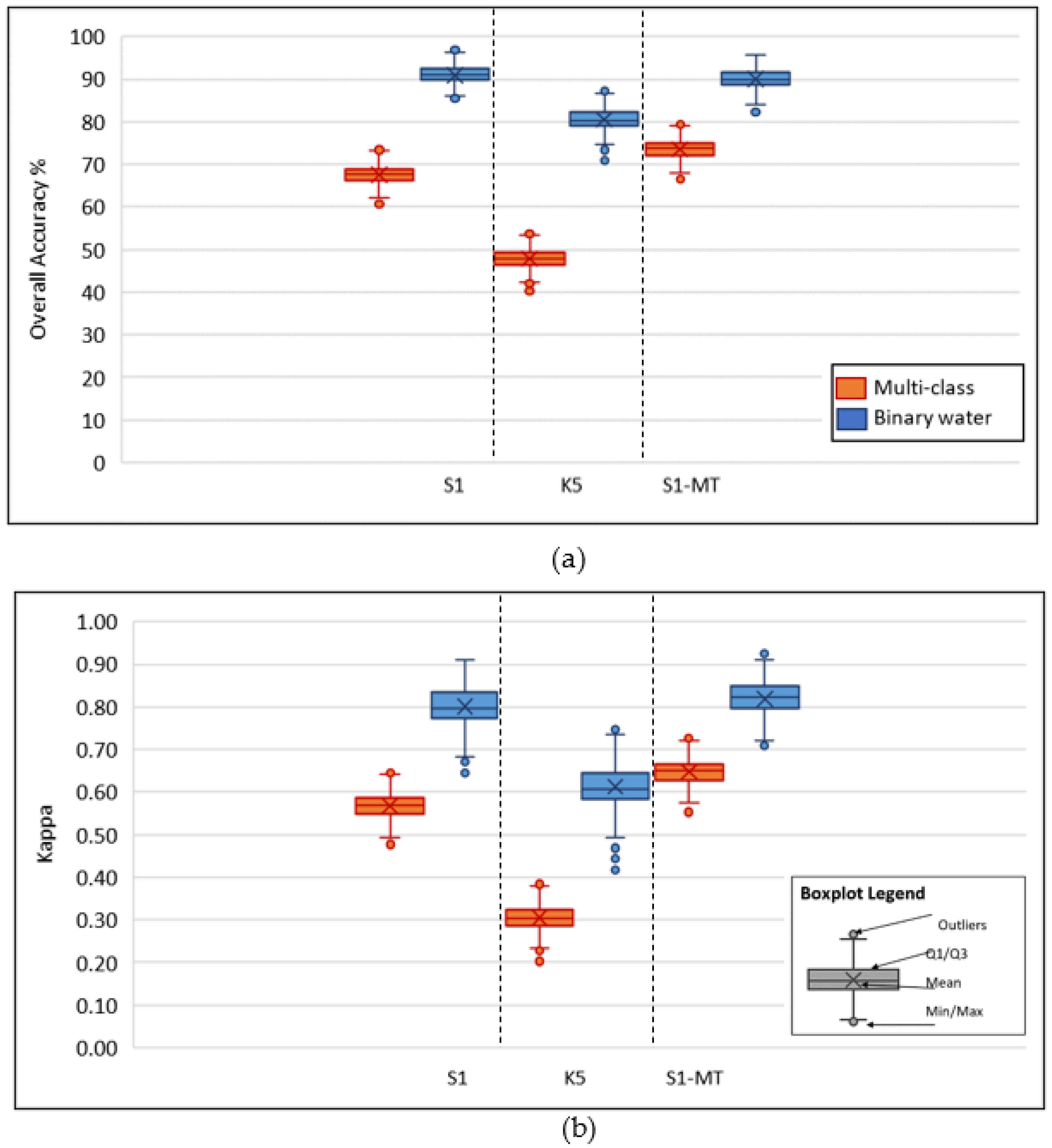
By comparing the classification results of the S1 sensor with those from K5, the difference in wavelength is evident. The X-band K5 imagery yielded significantly lower accuracies than the C-band S1 imagery. This may be due to the shorter wavelength of K5, which is less sensitive to differences in roughness between the land cover classes. To test this, an additional classification was performed with just the VH bands of S1 and S1-MT. The results showed that the overall accuracy and kappa coefficient results for Sentinel-1 VH are less accurate than using both polarizations, but they are still more accurate than the K5 results. There is also a bigger difference in overall accuracy and kappa coefficient for the multi-class classification scheme than the binary-water classification scheme. This further supports the notion that the C-band is better suited for this application than the X-band, even at a lower resolution.
The radiometric calibration of K5 may also influence the weaker results. Comparing multi-temporal filtering with single-date filtering showed that S1-MT performed more accurately, with margins of less than 3% in producer’s accuracy for the multi-class classification and margins of less than 2% in producer’s accuracy for the binary-water classification. Multi-temporal filtering reduces the amount of speckle, but the difference in UA and PA between S1 and S1-MT is negligible. This suggests that the time, data, and computation cost of performing multi-temporal filtering might not be worthwhile for this application.
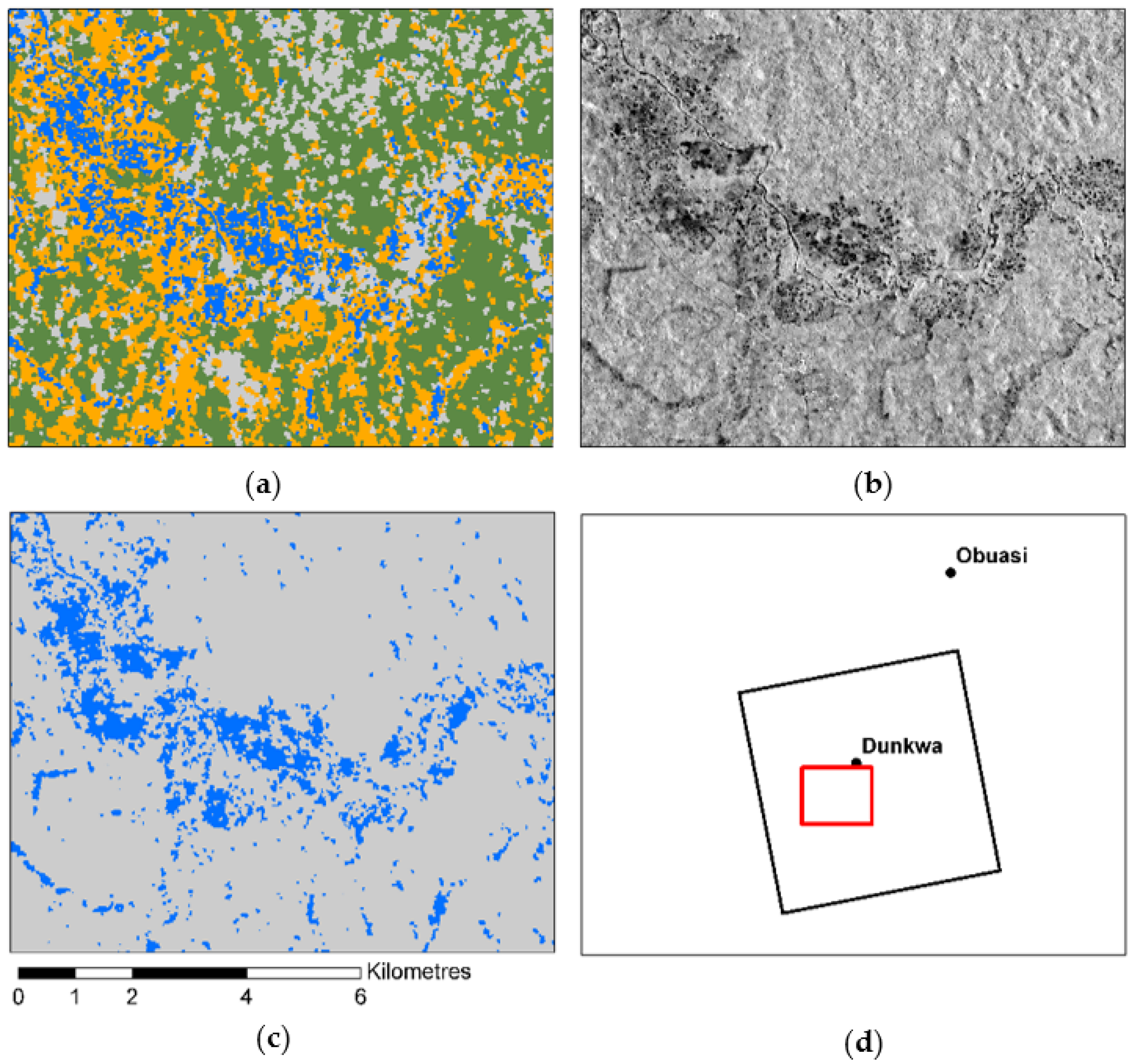
Confusion exists within the multi-class classification scheme, especially between water and bare ground. This is evident by the high omission and commission errors produced by this classification scheme. With the S1 imagery, the water class and the bare ground class are mixed at the ASM sites around the river, due to the use of lower resolution than the K5 imagery. Therefore, the binary-water classification scheme obtained significantly higher accuracies due to the elimination of confusion. This is confirmed by the low omission and commission errors of the binary-water classification scheme. The implication is that while small-scale mining operations cannot be directly detected using this approach, the scattered water pools associated with these operations can be detected to a fair degree of accuracy.
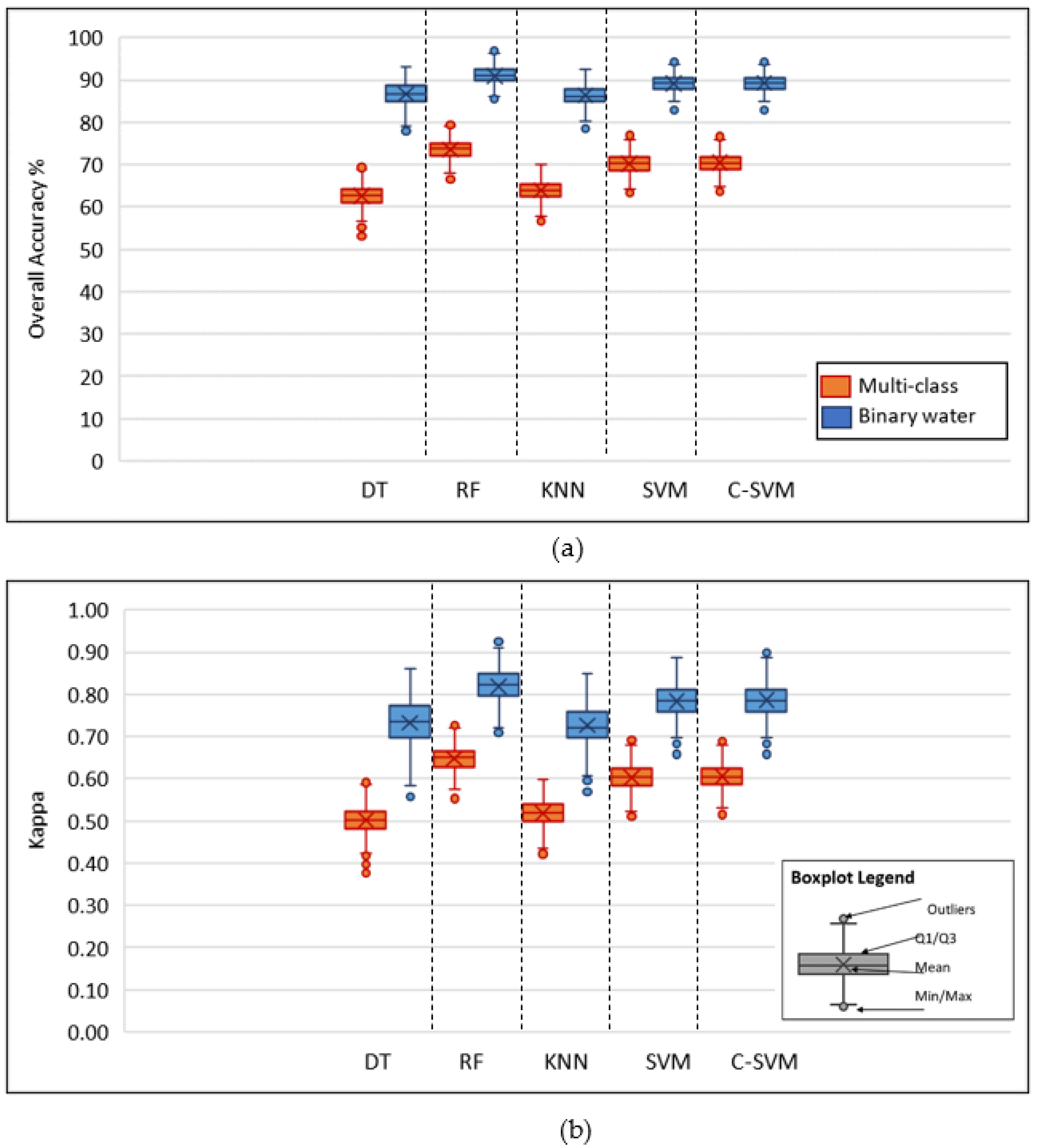
The same trend as in the SAR dataset comparison occurs in the machine learning comparison, where the binary-water classification scheme outperforms the multi-class classification scheme. The difference between the highest-performing dataset and lowest-performing dataset for the multi-class classification scheme is around 21%, whereas the difference for the binary-water classification scheme is around 10%. The difference between the highest performing classifier for the multi-class classification scheme is less than 11%, and the difference for the binary-water classification scheme is less than 7%. The high variance in the multi-class classification scheme results is due to the misclassification of classes that took place during this classification process.
For the machine learning classifier comparison, the random forest classifier was significantly more accurate than the other classifiers, with a probability of 0.87 at a 95% confidence level. Random forest is the most robust of the machine learning algorithms and deals very well with high dimensionality and complex data. C-SVM and SVM also achieved high overall accuracies, where C-SVM outperformed SVM. This is likely because the data structure was of a higher dimensionality, where the C-SVM kernel could find a better fit for the hyperplane to group the data. The decision trees classifier gave the least accurate as well as the least reliable results. This is because of how the trees are split in the algorithm and not iterated through, unlike in the random forest method. KNN is the simplest of the algorithms and performed slightly better than decision trees. KNN is not robust, demonstrating high dimensionality and complex data.
In Ghana, the mapping of illegal mining using remote sensing has only been attempted in one study [15], where they used multi-temporal optical imagery. They were able to detect the galamsey sites with change detection in Ghana but recommended the use of SAR imagery because of the interference of cloud cover. Bangira et al. [45] compared different machine learning classifiers where they mapped different types of water bodies; the SVM classifier outperformed the RF classifier, with an average overall accuracy of 91.7% compared to 79.5%. Their study incorporated SAR imagery and optical imagery, as well as indices, into the training of the classifiers. The results from the classification conducted in this study showed that RF outperformed SVM. A likely reason that SVM performed better than RF in Bangira et al.’s [45] study is that the indices and optical imagery gave more information on the water body types, meaning that it was simpler for the SVM classifier to classify the data. RF is prone to overclassifying, and this may have been the case in their study. Bangira et al. [45] also assessed the Otsu threshold methods and made the point that for water body mapping, using thresholds is simpler and yields accurate enough results for classification. From studies where floods were mapped with SAR imagery (e.g., [41,89,90,91]), threshold methods were used, therefore suggesting that mapping SSM with thresholds is a simpler and more effective option.
The lower accuracies obtained from S1 using only the VH polarization, when compared to using both VH and VV, indicate that the combination of these polarizations increases the discriminatory power of the machine learning algorithms. Since the VH-only S1 classification outperformed the VH-only K5 classification, it can also be argued that the difference in accuracy obtained between these two sensors is largely due to the difference in wavelength and not due to the increased dimensionality offered by S1′s dual polarization. In a forested environment such as this, the C-band is therefore preferable to the X-band for mapping SSM.

5. Conclusions

The C-band Sentinel-1 image outperformed the X-band KompSAT-5 image in accuracy and reliability. The KompSAT-5 image performance was substandard for both classification schemes, with an OA of less than 60% and a kappa coefficient of less than 0.6. Both SAR sensors could only classify the water bodies associated with SSM. Both single-product speckle-filtered SAR and multi-temporally filtered SAR produced very accurate and reliable results. However, the multi-temporally filtered database had a smaller range in the difference between the results of the multi-class classification scheme and the binary-water classification scheme. For this reason, multi-temporal filtering improves the overall reliability of the classification results. The comparison of the machine learning classification algorithms showed that RF is the best-suited algorithm to map SSM with SAR imagery. However, SVM came a close second. The influence of the custom kernel for SVM was insignificant and can therefore be deemed unnecessary. The DT and KNN algorithms had the poorest performance and are not suitable for SSM mapping with SAR.
The classification methods showed that a multi-class classification approach for using SAR to map illegal mining in forested areas does not perform well. The binary-water classification scheme gave highly accurate and reliable results, especially with the multi-temporally filtered Sentinel-1 imagery and the random forest classifier. The resulting classifications only mapped the water bodies in the image and the actual SSM activities were not yet mapped. This is, however, very useful because of the association of illegal alluvial mining with water bodies.
This research has shown that C-band SAR imagery can be successfully used to detect illegal mining operations in tropical regions by means of the associated water bodies. SSM in these areas are remote and require an uninterrupted supply of remote sensing imagery to provide useful insights on the spatial distribution patterns of SSM activities. The methods tested in this study are a step toward achieving automated near-real-time monitoring of SSM in cloud-cover-prone areas. Freely available SAR imagery, such as from Sentinel-1, could serve as the cornerstone of an operational monitoring system designed to detect and monitor illegal mining operations.

Author Contributions

Conceptualization, G.J.v.R. and J.K.; data curation, G.J.v.R. and J.K.; formal analysis, G.J.v.R.; methodology, G.J.v.R.; project administration, G.J.v.R. and J.K.; supervision, J.K.; writing—original draft, G.J.v.R.; writing—review and editing, G.J.v.R. and J.K. All authors have read and agreed to the published version of the manuscript.

Funding

This research was funded by the Space Advisory Company with a research grant and the Council for Geoscience for G.J.v.R.’s study bursary.

Institutional Review Board Statement

Not applicable.

Informed Consent Statement

Not applicable.

Data Availability Statement

Publicly available datasets were analyzed in this study. These data can be found here: https://scihub.copernicus.eu/dhus/#/home (accessed on: 6 June 2018) and http://www.si-imaging.com/products/#1478507064219-34e51d03-67d9 (accessed on: 31 July 2018).

Acknowledgments

Thank you to Janine Cole and Patrick Cole at the CGS for their guidance and support, and SI-Imaging for providing the KompSAT-5 data. The authors also wish to thank the anonymous reviewers for their valuable inputs to the paper.

Conflicts of Interest

The authors declare that they have no known competing financial interests or personal relationships that could have appeared to influence the work reported in this paper.

Appendix A. Confusion Matrices for the Image Classifications

Table A1. Random forest multi-class classification on an S1 confusion matrix.
WaterVegetationBare GroundBuilt-UpTOTALPA %EO %
Water6701017985.0614.94
Vegetation15513117969.3230.68
Bare ground15163997949.2850.72
Built-up31410527966.4033.60
TOTAL85857274316
UA %78.6164.5254.2371.02
EC %21.3935.4845.7728.98
Overall accuracy67.51
Overall kappa0.57
Table A2. Random forest multi-class classification on a K5 confusion matrix.
WaterVegetationBare GroundBuilt-UpTOTALPA %EO %
Water5322047966.5833.42
Vegetation63316247941.3858.62
Bare ground251526127933.0666.94
Built-up42411407950.5849.42
TOTAL88747380316
UA %59.6543.8935.6349.93
EC %40.3556.1164.3750.07
Overall accuracy47.90
Overall kappa0.31
Table A3. Random forest multi-class classification on an S1-MT confusion matrix.
WaterVegetationBare GroundBuilt-UpTOTALPA %EO %
Water690917987.3412.66
Vegetation1571387972.4327.57
Bare ground12174557957.1342.87
Built-up387617977.4722.53
TOTAL85827475316
UA %81.2269.7061.1281.50
EC %18.7830.3038.8818.50
Overall accuracy73.60
Overall kappa0.65
Table A4. Decision trees multi-class classification on an S1-MT confusion matrix.
WaterVegetationBare GroundBuilt-UpTOTALPA %EO %
Water6021247976.4923.51
Vegetation24619127958.4241.58
Bare ground12193897948.3451.66
Built-up5129537967.3532.65
TOTAL79797979316
UA %76.6858.1348.1867.74
EC %23.3241.8751.8232.26
Overall accuracy62.65
Overall kappa0.50
Table A5. KNN multi-class classification on an S1-MT confusion matrix.
WaterVegetationBare GroundBuilt-UpTOTALPA %EO %
Water6521117981.6518.35
Vegetation4571447971.7628.24
Bare ground18223447942.8357.17
Built-up4199477959.1140.89
TOTAL911006857316
UA %70.9756.6149.4582.58
EC %29.0343.3950.5517.42
Overall accuracy62.65
Overall kappa0.50
Table A6. SVM multi-class classification on an S1-MT confusion matrix.
WaterVegetationBare GroundBuilt-UpTOTALPA %EO %
Water6511217982.0317.97
Vegetation1561677970.7129.29
Bare ground10174667958.1141.89
Built-up4127567970.8329.17
TOTAL79868170316
UA %81.8765.1856.5380.03
EC %18.1334.8243.4719.97
Overall accuracy70.42
Overall kappa0.61
Table A7. C-SVM multi-class classification on an S1-MT confusion matrix.
WaterVegetationBare GroundBuilt-UpTOTALPA %EO %
Water6611117983.4416.56
Vegetation2571557972.1227.88
Bare ground14174357954.2345.77
Built-up4118567970.8129.19
TOTAL86857868316
UA %76.9466.8455.2782.78
EC %23.0633.1644.7317.22
Overall accuracy62.65
Overall kappa0.50
Table A8. Random forest binary-water classification on an S1 confusion matrix.
WaterNon-WaterTOTALPA %EO %
Water7277991.448.56
Non-water9707988.6511.35
TOTAL8177158
UA %88.9691.19
EC %11.048.81
Overall accuracy90.93
Overall kappa0.80
Table A9. Random forest binary-water classification on a K5 confusion matrix.
WaterNon-WaterTOTALPA %EO %
Water65147981.9718.03
Non-water16637979.2520.75
TOTAL8177158
UA %79.8081.46
EC %20.2018.54
Overall accuracy80.61
Overall kappa0.61
Table A10. Random forest binary-water classification on an S1-MT confusion matrix.
WaterNon-WaterTOTALPA %EO %
Water7367993.026.98
Non-water9707988.8411.16
TOTAL8276158
UA %89.2992.71
EC %10.717.29
Overall accuracy90.04
Overall kappa0.82
Table A11. Decision trees binary-water classification on an S1-MT confusion matrix.
WaterNon-WaterTOTALPA %EO %
Water68117986.5813.42
Non-water10697986.7313.27
TOTAL7979158
UA %86.7186.60
EC %13.2913.40
Overall accuracy86.65
Overall kappa0.73
Table A12. KNN binary-water classification on an S1-MT confusion matrix.
WaterNon-WaterTOTALPA %EO %
Water69107986.8113.19
Non-water11687985.7914.21
TOTAL79.80578.195158
UA %85.9486.68
EC %14.0613.32
Overall accuracy86.30
Overall kappa0.73
Table A13. SVM binary-water classification on an S1-MT confusion matrix.
WaterNon-WaterTOTALPA %EO %
Water7187989.6910.31
Non-water9707988.9611.04
TOTAL8078158
UA %89.0489.61
EC %10.9610.39
Overall accuracy89.33
Overall kappa0.79
Table A14. C-SVM binary-water classification on an S1-MT confusion matrix.
WaterNon-WaterTOTALPA %EO %
Water7277991.358.65
Non-water10697986.9913.01
TOTAL82.44375.557158
UA %87.5390.95
EC %12.479.05
Overall accuracy89.17
Overall kappa0.78

References

  1. Hilson, G. Farming, small-scale mining and rural livelihoods in Sub-Saharan Africa: A critical overview. Extr. Ind. Soc. 2016, 3, 547–563. [Google Scholar] [CrossRef]
  2. Moomen, A.W.; Dewan, A. Assessing the spatial relationships between mining and land degradation: Evidence from Ghana. Int. J. Min. Reclam. 2017, 31, 505–518. [Google Scholar] [CrossRef]
  3. Shaw, T.M. African agency & quest; Africa, South Africa and the BRICS. Int. Politics 2015, 52, 255–268. [Google Scholar]
  4. Mantey, J.; Owusu-Nimo, F.; Nyarko, K.B.; Aubynn, A. Operational dynamics of ‘Galamsey’ within eleven selected districts of western region of Ghana. J. Min. Environ. 2017, 8, 11–34. [Google Scholar]
  5. Owusu-Nimo, F.; Mantey, J.; Nyarko, K.B.; Appiah-Effah, E.; Aubynn, A. Spatial distribution patterns of illegal artisanal small scale gold mining (Galamsey) operations in Ghana: A focus on the Western Region. Heliyon 2018, 4, e00534. [Google Scholar] [CrossRef] [PubMed] [Green Version]
  6. Aryee, B.N.A.; Ntibery, B.K.; Atorkui, E. Trends in the small-scale mining of precious minerals in Ghana: A perspective on its environmental impact. J. Clean. Prod. 2003, 11, 131–140. [Google Scholar] [CrossRef]
  7. Owusu, E.E.; Dwomoh, G. The Impact of Illegal Mining on the Ghanaian Youth: Evidence From Kwaebibirem District In Ghana. Res. Humanit. Soc. Sci. 2012, 2, 86–93. [Google Scholar]
  8. ‘GALAMSEY’ a Canker in Western Region. Available online: https://www.modernghana.com/news/472110/1/galamsey-a-canker-in-western-region.html (accessed on 16 March 2018).
  9. Aubynn, A. Sustainable solution or a marriage of inconvenience? The coexistence of large-scale mining and artisanal and small-scale mining on the Abosso Goldfields concession in Western Ghana. Resour. Policy 2009, 34, 64–70. [Google Scholar] [CrossRef]
  10. The Impact of Chinese Involvement in Small-Scale Gold Mining in Ghana. Available online: https://www.theigc.org/wp-content/uploads/2016/08/Crawford-et-al-2015-Final-Report-1.pdf (accessed on 25 April 2018).
  11. Galamsey Killing Oda Forest Reserve but Gov’t Looks Unconcerned. Available online: https://www.todaygh.com/galamsey-killing-oda-forest-reserve-govt-looks-unconcerned/ (accessed on 16 March 2018).
  12. Special Report: The Cost of Galamsey—Ghana Extractive Industries Transparency Initiative. Available online: http://www.gheiti.gov.gh/site/index.php?option=com_content&view=article&id=187:special-report-the-cost-of-galamsey&catid=1:latest-news&Itemid=29 (accessed on 17 March 2018).
  13. Residents Worried over Abandoned Galamsey Pits. Available online: https://www.ghanaweb.com/GhanaHomePage/regional/Residents-worried-over-abandoned-galamsey-pits-467469 (accessed on 16 March 2018).
  14. Asner, G.P.; Llactayo, W.; Tupayachi, R.; Luna, E.R. Elevated rates of gold mining in the Amazon revealed through high-resolution monitoring. Proc. Natl. Acad. Sci. USA 2013, 110, 18454–18459. [Google Scholar] [CrossRef] [PubMed] [Green Version]
  15. Snapir, B.; Simms, D.M.; Waine, T.W. Mapping the expansion of galamsey gold mines in the cocoa growing area of Ghana using optical remote sensing. Int. J. Appl. Earth Obs. Geoinf. 2017, 58, 225–233. [Google Scholar] [CrossRef] [Green Version]
  16. Mansourpour, M.; Rajabi, M.A.; Blais, J.A.R. Effects and Performance of Speckle Noise Reduction Filters on Active Radar and SAR Images. ISPRS Int. J. Geo-Inf. 2006, 36, 1–6. [Google Scholar]
  17. Joshi, N.; Baumann, M.; Ehammer, A.; Fensholt, R.; Grogan, K.; Hostert, P.; Jepsen, M.R.; Kuemmerle, T.; Meyfroidt, P.; Mitchard, E.T.A.; et al. A review of the application of optical and radar remote sensing data fusion to land use mapping and monitoring. Remote Sens. 2016, 8, 70. [Google Scholar] [CrossRef] [Green Version]
  18. Reiche, J.; Hamunyela, E.; Verbesselt, J.; Hoekman, D.; Wageningen, M.H. Improving near-real-time deforestation monitoring in tropical dry forests by combining dense Sentinel-1 time series with Landsat and ALOS-2 PALSAR-2. Remote Sens. Environ. 2018, 204, 147–161. [Google Scholar] [CrossRef]
  19. Forkuor, G.; Ullmann, T.; Griesbeck, M. Mapping and monitoring small-scale mining activities in Ghana using Sentinel-1 time series (2015–2019). Remote Sens. 2020, 12, 911. [Google Scholar] [CrossRef] [Green Version]
  20. Denner, M.G. The Application of Synthetic Aperture Radar for the Detection and Mapping of Small-Scale Mining in Ghana. Master’s Thesis, Stellenbosch University, Cape Town, South Africa, 2020. [Google Scholar]
  21. Dewan, A.M.; Kankam-Yeboah, K.; Nishigaki, M. Using Synthetic Aperture Radar (SAR) Data for Mapping River Water Flooding in an Urban Landscape: A Case Study of Greater Dhaka, Bangladesh. J. Japan Soc. Hydrol. Water Resour. 2006, 19, 44–54. [Google Scholar] [CrossRef] [Green Version]
  22. Yousif, O.; Ban, Y. Improving SAR-Based Urban Change Detection by Combining MAP-MRF Classifier and Nonlocal Means Similarity Weights. IEEE J. Sel. Top. Appl. Earth Obs. Remote Sens. 2014, 7, 4288–4300. [Google Scholar] [CrossRef]
  23. White, L.; Brisco, B.; Dabboor, M.; Schmitt, A.; Pratt, A. A Collection of SAR Methodologies for Monitoring Wetlands. Remote Sens. 2015, 7, 7615–7645. [Google Scholar] [CrossRef] [Green Version]
  24. Molijn, R.A.; Iannini, L.; Vieira Rocha, J.; Hanssen, R.F. Sugarcane Productivity Mapping through C-Band and L-Band SAR and Optical Satellite Imagery. Remote Sens. 2019, 11, 1109. [Google Scholar] [CrossRef] [Green Version]
  25. Marghany, M.; Sabu, Z.; Hashim, M. Mapping coastal geomorphology changes using synthetic aperture radar data. Int. J. Phys. Sci. 2010, 5, 1890–1896. [Google Scholar]
  26. Han, H.; Hong, S.H.; Kim, H.C.; Chae, T.B.; Choi, H.J. A study of the feasibility of using KOMPSAT-5 SAR data to map sea ice in the Chukchi Sea in late summer. Remote Sens. Lett. 2017, 8, 468–477. [Google Scholar] [CrossRef]
  27. Parihar, N.; Das, A.; Rathore, V.S.; Nathawat, M.S.; Mohan, S. Analysis of L-band SAR backscatter and coherence for delineation of land-use/land-cover. Int. J. Remote Sens. 2014, 35, 6781–6798. [Google Scholar] [CrossRef]
  28. Pu, W. Shuffle GAN With Autoencoder: A Deep Learning Approach to Separate Moving and Stationary Targets in SAR Imagery. IEEE Trans. Neural Netw. Learn. 2021, 1, 1–15. [Google Scholar] [CrossRef]
  29. Chen, K.S.; Huang, W.P.; Tsay, D.H.; Amar, F. Classification of multifrequency polarimetric SAR imagery using a dynamic learning neural network. IEEE Trans. Geosci. Remote Sens. 1996, 34, 814–820. [Google Scholar] [CrossRef]
  30. Rodriguez-Galiano, V.F.; Ghimire, B.; Rogan, J.; Chica-Olmo, M.; Rigol-Sanchez, J.P. An assessment of the effectiveness of a random forest classifier for land-cover classification. ISPRS J. Photogramm. Remote Sens. 2012, 67, 93–104. [Google Scholar] [CrossRef]
  31. Pierce, L.E.; Dobson, M.C.; Ulaby, F. Knowledge-based land-cover classification using ERS-l/JERS-1 composites. In Proceedings of the IGARSS ’94—1994 IEEE International Geoscience and Remote Sensing Symposium, Pasadena, CA, USA, 8–12 August 1994. [Google Scholar]
  32. Bala, G.; Caldeira, K.; Wickett, M.; Phillips, T.; Lobell, D.; Delire, C.; Mirin, A. Combined climate and carbon-cycle effects of large-scale deforestation. Proc. Natl. Acad. Sci. USA 2007, 104, 6550–6555. [Google Scholar] [CrossRef] [PubMed] [Green Version]
  33. Lambin, E.; Turner, B.; Geist, H.; Agbola, S.; Angelsen, A.; Bruce, J.; Coomes, O.; Dirzo, R.; Fischer, G.; Folke, C. The causes of land-use and land-cover change: Moving beyond the myths. Glob. Environ. 2001, 11, 261–269. [Google Scholar] [CrossRef]
  34. Mas, J.F.; Velázquez, A.; Díaz-Gallegos, J.R.; Mayorga-Saucedo, R.; Alcántara, C.; Bocco, G.; Castro, R.; Fernández, T.; Pérez-Vega, A. Assessing land use/cover changes: A nationwide multidate spatial database for Mexico. Int. J. Appl. Earth Obs. Geoinf. 2004, 5, 249–261. [Google Scholar] [CrossRef]
  35. Turner, B.; Lambin, E.; Reenberg, A. The emergence of land change science for global environmental change and sustainability. Proc. Natl. Acad. Sci. USA 2007, 104, 20666–20671. [Google Scholar] [CrossRef] [PubMed] [Green Version]
  36. Elmes, A.; Ipanaqué, J.G.Y.; Rogan, J.; Cuba, N.; Bebbington, A. Mapping licit and illicit mining activity in the Madre de Dios region of Peru. Remote Sens. Lett. 2014, 5, 882–891. [Google Scholar] [CrossRef]
  37. Waske, B.; Van der Linden, S. Classifying multilevel imagery from SAR and optical sensors by decision fusion. IEEE Trans. Geosci. Remote Sens. 2008, 46, 1457–1466. [Google Scholar] [CrossRef]
  38. Hilson, G.; Hilson, A.; Maconashie, R.; McQuilken, J.; Goumandakoye, H. Artisanal and small-scale mining (ASM) in sub-Saharan Africa: Re-conceptualizing formalization and “illegal” activity. Geoforum 2017, 83, 80–90. [Google Scholar] [CrossRef]
  39. Ban, Y.; Wu, Q. RADARSAT SAR Data for Landuse/Land-Cover Classification in the Rural-Urban Fringe of the Greater Toronto Area. In Proceedings of the 8th AGILE International Conference on Geographic Information Science, Denver, CO, USA, 24–29 July 2005. [Google Scholar]
  40. Ban, Y.; Hu, H.; Rangel, I.M. Fusion of Quickbird MS and RADARSAT SAR data for urban land cover mapping: Object-based and knowledge-based approach. Int. J. Remote Sens. 2010, 31, 1391–1410. [Google Scholar] [CrossRef]
  41. Schlaffer, S.; Matgen, P.; Hollaus, M.; Wagner, W. Flood detection from multi-temporally SAR data using harmonic analysis and change detection. Int. J. Appl. Earth Obs. Geoinf. 2015, 38, 15–24. [Google Scholar] [CrossRef]
  42. Schlaffer, S.; Chini, M.; Giustarini, L.; Matgen, P. Probabilistic mapping of flood-induced backscatter changes in SAR time series. Int. J. Appl. Earth Obs. Geoinf. 2017, 56, 77–87. [Google Scholar] [CrossRef]
  43. Fu, B.; Wang, Y.; Campbell, A.; Li, Y.; Zhang, B.; Yin, S.; Xing, Z.; Jin, X. Comparison of object-based and pixel-based Random Forest algorithm for wetland vegetation mapping using high spatial resolution GF-1 and SAR data. Ecol. Indic. 2017, 73, 105–117. [Google Scholar] [CrossRef]
  44. Mahdianpari, M.; Salehi, B.; Mohammadimanesh, F.; Motagh, M. Random forest wetland classification using ALOS-2 L-band, RADARSAT-2 C-band, and TerraSAR-X imagery. ISPRS J. Photogramm. Remote Sens. 2017, 130, 13–31. [Google Scholar] [CrossRef]
  45. Bangira, T.; Alfieri, S.M.; Menenti, M.; Van Niekerk, A. Comparing thresholding with machine learning classifiers for mapping complex water. Remote Sens. 2019, 11, 1351. [Google Scholar] [CrossRef] [Green Version]
  46. Hilson, G. A contextual review of the Ghanaian small-scale mining industry. Min. Miner. Sustain. Dev. 2001, 76, 29. [Google Scholar]
  47. Teschner, B.A. Small-scale mining in Ghana: The government and the galamsey. Resour. Policy 2012, 37, 308–314. [Google Scholar] [CrossRef]
  48. Corbett, T.; O’Faircheallaigh, C.; Regan, A. “Designated areas” and the regulation of artisanal and small-scale mining. Land Use Policy 2017, 68, 393–401. [Google Scholar] [CrossRef]
  49. Vogel, C.; Musamba, J.; Radley, B. A miner’s canary in eastern Congo: Formalisation of artisanal 3T mining and precarious livelihoods in South Kivu. Extr. Ind. Soc. 2018, 5, 73–80. [Google Scholar] [CrossRef]
  50. Hilson, G.; Goumandakoye, H.; Diallo, P. Formalizing artisanal mining “spaces” in rural sub-Saharan Africa: The case of Niger. Land Use Policy 2019, 80, 259–268. [Google Scholar] [CrossRef]
  51. Pedersen, R.H.; Mutagwabab, W.; Jønssonc, J.B.; Schoneveldd, G.; Jacobe, T.; Chachag, M.; Wengh, X.; Njau, M.G. Mining-sector dynamics in an era of resurgent resource nationalism: Changing relations between large-scale mining and artisanal and small-scale mining in Tanzania. Resour. Policy 2019, 62, 339–346. [Google Scholar] [CrossRef]
  52. Otamonga, J.P.; Poté, J.W. Abandoned mines and artisanal and small-scale mining in Democratic Republic of the Congo (DRC): Survey and agenda for future research. J. Geochem. Explor. 2020, 208, 106394. [Google Scholar] [CrossRef]
  53. Veiga, M.M.; Maxson, P.A.; Hylander, L.D. Origin and consumption of mercury in small-scale gold mining. J. Clean. Prod. 2006, 14, 436–447. [Google Scholar] [CrossRef]
  54. Emmanuel, A. Impact of Illegal Mining on Water Resources for Domestic and Irrigation Purposes. ARPN J. Earth Sci. 2013, 2, 117–121. [Google Scholar]
  55. Clifford, M.J. Assessing releases of mercury from small-scale gold mining sites in Ghana. Extr. Ind. Soc. 2017, 4, 497–505. [Google Scholar] [CrossRef]
  56. Gyamfi, E.; Appiah-Adjei, E.K.; Adjei, K.A. Potential heavy metal pollution of soil and water resources from artisanal mining in Kokoteasua, Ghana. Groundw. Sustain. Dev. 2019, 8, 450–456. [Google Scholar] [CrossRef]
  57. Moody, K.H.; Hasan, K.M.; Aljic, S.; Blakeman, V.M.; Hicks, L.P.; Loving, D.C.; Moore, M.E.; Hammett, B.S.; Silva-González, M.; Seney, C.S.; et al. Mercury emissions from Peruvian gold shops: Potential ramifications for Minamata compliance in artisanal and small-scale gold mining communities. Environ. Res. 2019, 182, 109042. [Google Scholar] [CrossRef]
  58. Knoblauch, A.M.; Farnham, A.; Ouoba, J.; Zanetti, J.; Müller, S.; Jean-Richard, V.; Utzinger, J.; Wehrli, B.; Brugger, F.; Diagbouga, S.; et al. Potential health effects of cyanide use in artisanal and small-scale gold mining in Burkina Faso. J. Clean. Prod. 2020, 252, 119689. [Google Scholar] [CrossRef]
  59. Kranz, O.; Lang, S.; Schoepfer, E. 2.5D change detection from satellite imagery to monitor small-scale mining activities in the Democratic Republic of the Congo. Int. J. Appl. Earth Obs. Geoinf. 2017, 61, 81–91. [Google Scholar] [CrossRef]
  60. Almeida-Filho, R.; Shimabukuro, Y.E. Detecting areas disturbed by gold mining activities through JERS-1 SAR images, Roraima State, Brazilian Amazon. Int. J. Remote Sens. 2000, 21, 3357–3362. [Google Scholar] [CrossRef]
  61. Saatchi, S.S.; Soares, J.V.; Alves, D.S. Mapping deforestation and land use in Amazon rainforest by using SIR-C imagery. Remote Sens. Environ. 1997, 59, 191–202. [Google Scholar] [CrossRef]
  62. Shimabukuro, Y.E.; Amaral, S.; Ahern, F.J.; Pietsch, R.W. Land cover classification from RADARSAT data of the Tapajós National Forest, Brazil. Can. J. Remote Sens. 1998, 24, 393–401. [Google Scholar] [CrossRef]
  63. Dutra, L.V.; Hernandez, F.P.; Mazzocato, M.E.; Souza, R.C.M.; Oliveira, C. Land cover classification based on multi-date JERS-1 imagery as a basis for deforestation detection. In Proceedings of the IEEE 1999 International Geoscience and Remote Sensing Symposium. IGARSS’99 (Cat. No.99CH36293), Hamburg, Germany, 28 June–2 July 1999. [Google Scholar]
  64. Climate and Average Weather in Ghana. Available online: https://weather-and-climate.com/average-monthly-Rainfall-Temperature-Sunshine-in-Ghana (accessed on 22 December 2019).
  65. Ghana: Geography, Location, Weather etc. 2019. Available online: https://www.ghanaweb.com/GhanaHomePage/geography/climate.php (accessed on 15 July 2019).
  66. Hirose, K.; Maruyama, Y.; Do Van, Q.; Tsukada, M.; Shiokawa, Y. Visualization of flood monitoring in the lower reaches of the Mekong River. In Proceedings of the 22nd Asian Conference on Remote Sensing, Singapore, 5–9 November 2001. [Google Scholar]
  67. Yamada, Y. Detection of flood-inundated area and relation between the area and micro-geomorphology using SAR and GIS. In IGARSS 2001. Scanning the Present and Resolving the Future, Proceedings of the IEEE 2001 International Geoscience and Remote Sensing Symposium (Cat. No.01CH37217), Sydney, Australia, 9–13 July 2001; IEEE: Sydney, Australia, 2001. [Google Scholar]
  68. Matgen, P.; Hostache, R.; Schumann, G.; Pfister, L.; Hoffmann, L.; Savenije, H. Towards an automated SAR-based flood monitoring system: Lessons learned from two case studies. Phys. Chem. Earth 2011, 36, 241–252. [Google Scholar] [CrossRef]
  69. Giustarini, L.; Hostache, R.; Matgen, P.; Schumann, G.; Bates, P.D.; Mason, D.C. A Change detection approach to flood mapping in urban areas using TerraSAR-X. IEEE Trans. Geosci. Remote Sens. 2013, 51, 2417–2430. [Google Scholar] [CrossRef] [Green Version]
  70. Tan, Q.; Bi, S.; Hu, J.; Liu, Z. Measuring lake water level using multi-source remote sensing images combined with hydrological statistical data. In Science for Society: Exploring and Managing a Changing Planet, 2004, Proceedings of the International Geoscience and Remote Sensing Symposium, Anchorage, AK, USA, 20–24 September 2004; IEEE: Anchorage, AK, USA, 2004. [Google Scholar]
  71. Martinis, S.; Twele, A.; Voigt, S. Towards operational near real-time flood detection using a split-based automatic thresholding procedure on high-resolution TerraSAR-X data. Nat. Hazards Earth Syst. Sci. 2009, 9, 303–314. [Google Scholar] [CrossRef]
  72. Shen, X.; Anagnostoua, E.N.; Allenc, G.H.; Brakenridged, G.R.; Kettnerd, A.J. Near-real-time non-obstructed flood inundation mapping using synthetic aperture radar. Remote Sens. Environ. 2019, 221, 302–315. [Google Scholar] [CrossRef]
  73. Martinis, S.; Rieke, C. Backscatter analysis using multi-temporally and multi-frequency SAR data in the context of flood mapping at River Saale, Germany. Remote Sens. 2015, 7, 7732–7752. [Google Scholar] [CrossRef] [Green Version]
  74. Quegan, S.; Toan, T.L.; Yu, J.J.; Ribbes, F.; Floury, N. Multitemporal ERS SAR analysis applied to forest mapping. IEEE Trans. Geosci. Remote Sens. 2000, 38, 741–753. [Google Scholar] [CrossRef]
  75. Verhulp, J.; Van Niekerk, A. Transferability of decision trees for land cover classification in a heterogeneous area. S. Afr. J. Geomat. 2017, 6, 30–46. [Google Scholar] [CrossRef]
  76. Breiman, L. Random forests. Mach. Learn. 2001, 45, 5–32. [Google Scholar] [CrossRef] [Green Version]
  77. Myburgh, G.; Van Niekerk, A. Impact of training set size on object-based landcover classification: A comparison of three classifiers. IJAGR 2014, 5, 49–67. [Google Scholar]
  78. Pedregosa, F.; Varoquaux, G.; Gramfort, A.; Michel, V.; Thirion, B. Scikit-learn: Machine Learning in Python. J. Mach. Learn. Res. 2011, 12, 2825–2830. [Google Scholar]
  79. User Guide for Scikit Learn Version 0.12. Scikit Learn User Guide 0.12. Available online: https://www.scribd.com/document/205251894/Scikit-Learn-User-Guide-0-12 (accessed on 12 June 2019).
  80. Cortes, C.; Vapnik, V. Support-Vector Networks. Mach. Learn. 1995, 20, 273–297. [Google Scholar] [CrossRef]
  81. Hwang, J.I.; Jung, H.S. Automatic Ship Detection Using the Artificial Neural Network and Support Vector Machine from X-Band SAR Satellite Images. Remote Sens. 2018, 10, 1799. [Google Scholar] [CrossRef] [Green Version]
  82. Chen, P.H.; Lin, C.J.; Schölkopf, B. A tutorial on ν-support vector machines. Appl. Stoch. Model. Bus. Ind. 2005, 21, 111–136. [Google Scholar] [CrossRef]
  83. A Practical Guide to Support Vector Classification. Available online: https://www.csie.ntu.edu.tw/~cjlin/papers/guide/guide.pdf (accessed on 12 June 2019).
  84. Support Vector Machines in Scikit-Learn. Available online: https://www.datacamp.com/community/tutorials/svm-classification-scikit-learn-python (accessed on 12 June 2019).
  85. Congalton, R.G.; Oderwald, R.G.; Mead, R.A. Assessing Landsat Classification Accuracy Using Discrete Multivariate Analysis Statistical Techniques. Photogramm. Eng. 1983, 49, 1671–1678. [Google Scholar]
  86. Foody, G.M. Explaining the unsuitability of the kappa coefficient in the assessment and comparison of the accuracy of thematic maps obtained by image classification. Remote Sens. Environ. 2020, 239, 111630. [Google Scholar] [CrossRef]
  87. Gilbertson, J.K.; Van Niekerk, A. Value of dimensionality reduction for crop differentiation with multi-temporal imagery and machine learning. Comput. Electron. Agric. 2017, 142, 50–58. [Google Scholar] [CrossRef]
  88. Statistics How to 2019. Z-Table (Right of Curve or Left)—Statistics How to [Online]. Available online: https://www.statisticshowto.datasciencecentral.com/tables/z-table/ (accessed on 27 June 2019).
  89. Long, S.; Fatoyinbo, T.E.; Policelli, F. Flood extent mapping for Namibia using change detection and thresholding with SAR. Environ. Res. Lett. 2014, 9, 035002. [Google Scholar] [CrossRef]
  90. Mason, D.C.; Guistarini, L.; Garcia-Pintado, J.; Cloke, H.L. Detection of flooded urban areas in high-resolution Synthetic Aperture Radar images using double scattering. Int. J. Appl. Earth Obs. Geoinf. 2014, 28, 150–159. [Google Scholar] [CrossRef] [Green Version]
  91. Clement, M.A.; Kilsby, C.G.; Moore, P. Multi-temporally synthetic aperture radar flood mapping using change detection. J. Flood Risk Manag. 2018, 11, 152–168. [Google Scholar] [CrossRef]
Figure 1. The footprints of the satellite imagery used in this study are located in Southern Ghana. All the imagery was cropped to the KompSAT-5 footprint that delineates the study area.
Remotesensing 14 00977 g001
Figure 2. Example subsets of imagery used: (a) Sentinel-1 VH backscatter from 8 August 2018, (b) KompSAT-5 VH backscatter from 12 July 2018, and (c) Sentinel-2 true-color image taken on 5 August 2018, where (d) gives the extent of the example subset area The example area highlights a section of the Ofin River where abundant small-scale mining takes place.
Remotesensing 14 00977 g002
Figure 3. Flowchart of the supervised classification method followed in this study.
Remotesensing 14 00977 g003
Figure 4. Graphs displaying the overall accuracy (a) and kappa coefficient (b) results for the SAR datasets comparison (image classification, part 1).
Remotesensing 14 00977 g004
Figure 5. Graphs displaying the overall accuracy (a) and kappa coefficient (b) results for the machine learning classifier comparison (image classification part 2).
Remotesensing 14 00977 g005
Figure 6. Example of the visual RF results of S1-MT where: (a) is the multi-class classification, (b) the intensity of S1-multi, (c) the binary water classification, and (d) the map showing the extent of the images in (ac). Blue is water, green is vegetation, orange is bare ground and grey is built-up area.
Remotesensing 14 00977 g006
Table 1. The descriptions of each class.
Multi-Class ClassesBinary-Water ClassesDescription
WaterWaterUniform texture. Blue, green pixels.
Built-up areaNon-waterBuilt structures such as roads, dam walls and buildings. Can be grey in color or brown.
VegetationForest: Densely packed trees. usually of a dark green color. Have a “speckled” texture.
Low vegetation: Usually located in patches of lighter green areas between darker green (forest/tree) areas. Vegetation refers to grass, bushes, and low trees.
Bare groundOpen areas that contain no structures or vegetation. Typically, a dark brown/brown/orange color or grey color.
Table 2. Summary of the image features used as input for the classification analysis. (S1 = single-date Sentinel-1, K5 = single-date KompSAT-5, S1-MT = multi-temporally filtered Sentinel-1).
ImageBackscatter BandsTexture FeaturesGeometric AttributesTotal Number of Features
S1VH, VV (n = 2)(n = 16)(n = 5)23
K5VH (n = 1)(n = 8)(n = 5)14
S1-MTVH, VV (n = 2)(n = 16)(n = 5)23
Table 3. Producer’s (PA) and user’s accuracies (UA) of the “water” class for RF classification on the S1, K5, and S1-MT datasets.
DatasetClassification Scheme
Multi-ClassBinary-Water
PA %UA %PA %UA %
S185.0678.6191.4488.96
K566.5859.6581.9779.80
S1-MT87.3481.2293.0289.29
Table 4. The average omission error and commission errors are presented in percentage for each dataset and classification scheme (OE: omission error; CE: commission error).
DatasetClassification Scheme
Multi-ClassBinary-Water
OE %CE %OE %CE %
RF S132.4932.919.969.93
RF S1-MT26.4026.629.079.00
RF K552.1052.7219.3919.39
Table 5. The significance evaluation results for each classifier are given, with the probability that was obtained through the area under the curve method.
OA Multi-ClassDTRFKNNC-SVMSVMMEAN (µ)STD DEV (σ)
Average OA of each classifier (%)62.3773.5463.7970.1770.3668.054.75
z-value−1.191.16−0.900.450.49
Area (probability)0.120.870.190.670.68
Table 6. Producer’s (PA) and user’s accuracies (UA) of the “water” class classification on S1-MT of DT, RF, KNN, SVM, and C-SVM.
ClassifierClassification Scheme
Multi-ClassBinary-Water
PA %UA %PA %UA %
DT76.4976.6886.5886.71
RF87.3481.2293.0289.29
KNN81.6570.9786.8185.94
SVM82.0381.8789.6989.04
C-SVM83.4476.9491.3587.53
Table 7. A summary of the averaged values for the results of Experiments 1 and 2.
Classifier/DatasetClassification Scheme
Multi-ClassBinary-Water
OA %KOA %K
RF K547.900.3180.610.61
RF S167.510.5790.930.80
RF S1-MT73.600.6590.040.82
DT62.650.5086.650.73
SVM70.420.6189.330.79
C-SVM70.150.6089.170.78
KNN63.840.5286.300.73
Average65.150.5487.580.75
Publisher’s Note: MDPI stays neutral with regard to jurisdictional claims in published maps and institutional affiliations.

