Panoptic Segmentation Meets Remote Sensing

Abstract

Panoptic segmentation combines instance and semantic predictions, allowing the detection of countable objects and different backgrounds simultaneously. Effectively approaching panoptic segmentation in remotely sensed data is very promising since it provides a complete classification, especially in areas with many elements as the urban setting. However, some difficulties have prevented the growth of this task: (a) it is very laborious to label large images with many classes, (b) there is no software for generating DL samples in the panoptic segmentation format, (c) remote sensing images are often very large requiring methods for selecting and generating samples, and (d) most available software is not friendly to remote sensing data formats (e.g., TIFF). Thus, this study aims to increase the operability of panoptic segmentation in remote sensing by providing: (1) a pipeline for generating panoptic segmentation datasets, (2) software to create deep learning samples in the Common Objects in Context (COCO) annotation format automatically, (3) a novel dataset, (4) leverage the Detectron2 software for compatibility with remote sensing data, and (5) evaluate this task on the urban setting. The proposed pipeline considers three inputs (original image, semantic image, and panoptic image), and our software uses these inputs alongside point shapefiles to automatically generate samples in the COCO annotation format. We generated 3400 samples with 512 × 512 pixel dimensions and evaluated the dataset using Panoptic-FPN. Besides, the metric analysis considered semantic, instance, and panoptic metrics, obtaining 93.865 mean intersection over union (mIoU), 47.691 Average (AP) Precision, and 64.979 Panoptic Quality (PQ). Our study presents the first effective pipeline for generating panoptic segmentation data for remote sensing targets.

1. Introduction

The increasing availability of satellite images alongside computational improvements makes the remote sensing field conducive to using deep learning (DL) techniques [1]. Unlike traditional machine learning (ML) methods for image classification that rely on a per-pixel analysis [2,3], DL enables the understanding of shapes, contours, textures, among other characteristics, resulting in better classification and predictive performance. In this regard, convolutional neural networks (CNNs) were a game-changing method in DL and pattern recognition because of its ability to process multi-dimensional arrays [4]. CNNs apply convolutional kernels throughout the image resulting in feature maps, enabling low, medium, and high-level feature recognition (e.g., corners, parts of an object, and full objects, respectively) [5]. Besides, the development of new CNN architectures is a fast-growing field with novel and better architectures year after year, such as VGGnet [6], ResNet [7], AlexNet [8], ResNeXt [9], Efficient-net [10], among others.

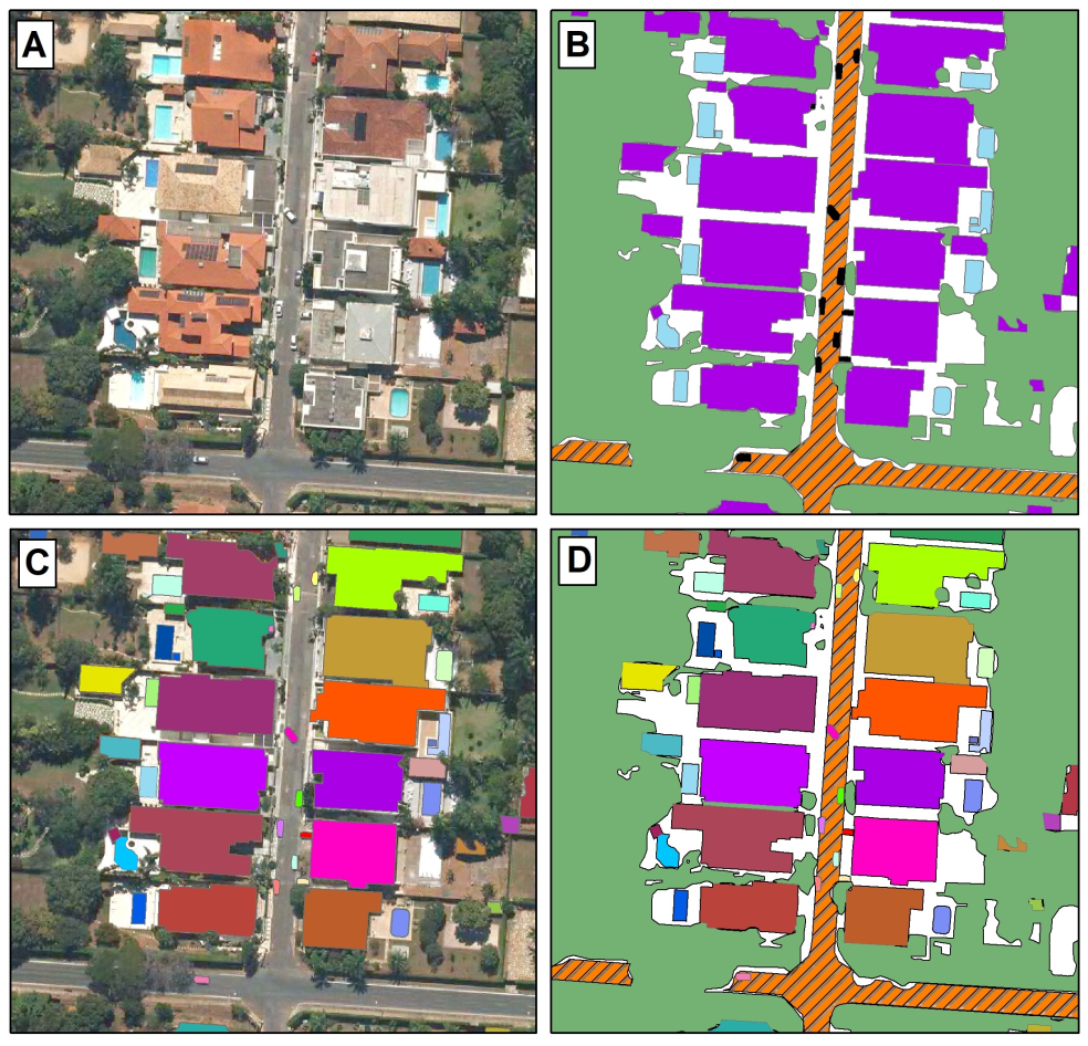
There are endless applications with CNN architectures, varying from single image classification to keypoint detection [11]. Nevertheless, there are three main approaches for image segmentation [1,12,13,14] (Figure 1: (1) semantic segmentation; (2) instance segmentation; and (3) panoptic segmentation. For a given input image (Figure 1A), semantic segmentation models perform a pixel-wise classification [15] (Figure 1B), in which all elements belonging to the same class receive the same label. However, this method presents limitations for the recognition of individual elements, especially in crowded areas. On the other hand, instance segmentation generates bounding boxes (i.e., a set of four coordinates that delimits the object’s boundaries) and performs a binary segmentation mask for each element, enabling a distinct identification [16]. Nonetheless, instance segmentation approaches are restricted to objects (Figure 1B), not covering background elements (e.g., lake, grass, roads). Most datasets adopt a terminology of “thing” and “stuff” categories to differentiate objects and backgrounds [17,18,19,20,21]. The “thing” categories are often countable and present characteristic shapes, similar sizes, and identifiable parts (e.g., buildings, houses, swimming pools). Oppositely, “stuff” categories are usually not countable and amorphous (e.g., lake, grass, roads) [22]. Thus, panoptic segmentation [23] aims to simultaneously combine instance and semantic predictions for classifying things and stuff categories, providing a more informative scene understanding (Figure 1D).

Although panoptic segmentation has excellent potential in remote sensing data, a crucial step for its expansion is the image annotation that varies according to the segmentation task. Semantic segmentation is the most straightforward approach, requiring the original image and their corresponding ground truth images. The instance segmentation has a more complicated annotation style, which requires the bounding box information, the class identification, and the polygons that constitute each object. A standard approach is to store all of this information in the Common Objects in Context (COCO) annotation format [20]. Panoptic segmentation has the most complex and laborious format, requiring instance and semantic annotations. Therefore, the high complexity of panoptic annotations leads to a lack of remote sensing databases. Currently, panoptic segmentation algorithms are compatible with the standard COCO annotation format [23]. A significant advantage of using the COCO annotation format is compatibility with state-of-the-art software. Nowadays, Detectron2 [24] is one of the most advanced algorithms for instance and panoptic segmentation, and most research advances involve changes in the backbone structures, e.g., MobileNetV3 [25], EfficientPS [26], Res2Net [27]. Therefore, this format enables vast methodological advances. However, a big challenge in the application of remote sensing is the adaptation of algorithms to its peculiarities, which include the image format (e.g., GeoTIFF and TIFF) and the multiple channels (e.g., multispectral and time series), which differ from the traditional Red, Green, and Blue (RGB) images used in other fields of computer vision [28].

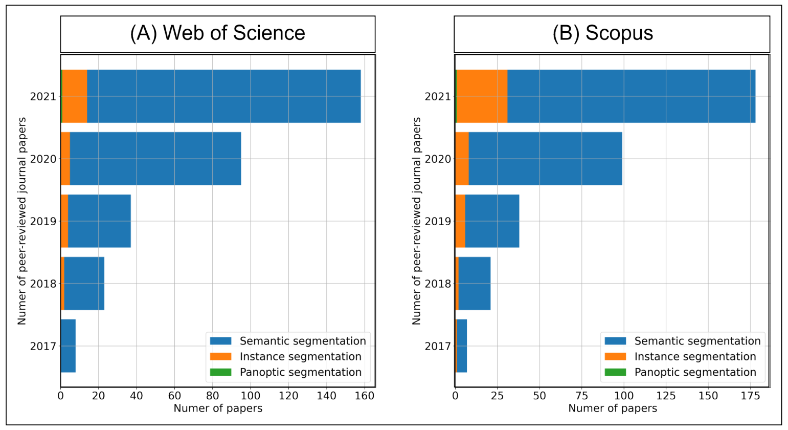
The increase in complexity among DL methods (panoptic segmentation > instance segmentation > semantic segmentation) reflects the frequency of peer-reviewed articles across each DL approach (Figure 2). On the web of science and scopus databases considering articles up to 1 January 2022, we evaluated four searches filtering by topic and only considering journal papers: (1) “remote sensing” AND “semantic segmentation” AND “deep learning”; (2) “remote sensing” AND “instance segmentation” AND “deep learning”; (3) “remote sensing” AND “panoptic segmentation” AND “deep learning” and (4) “panoptic segmentation”. Semantic segmentation is the most common approach using DL in remote sensing, while instance segmentation has significantly fewer papers. On the other hand, panoptic segmentation has only one research published in remote sensing [29], in which the authors used the DOTA [30], UCAS-AOD [31], and ISPRS-2D (https://www2.isprs.org/commissions/comm2/wg4/benchmark/semantic-labeling/, accessed on 25 January 2021) datasets, none of which are made for the panoptic segmentation task. Moreover, we found two other studies. The first focuses on change detection in building footprints using bi-temporal images [32], and the second use for different crops [33]. Although both studies implement panoptic models, it does not use “stuff” categories apart from the background, being very similar to an instance segmentation approach.

Even though the panoptic task is laborious, tools for easing the panoptic data preparation and integration with remote sensing peculiarities may present a significant breakthrough. The panoptic predictions retrieve countable objects and different backgrounds, guiding public policies and decision-making with complete information. The absence of remote sensing panoptic segmentation research alongside databases for this task represents a substantial gap. Moreover, One of the notable drawbacks in the computer vision community regarding traditional images is the inference time, which exalts models like YOLACT and YOLACT++ [34,35] due to the ability to handle real data time, even compromising the accuracy metrics a little. This problem is less significant in remote sensing as the image acquisition frequency is days, weeks, or even months, making it preferable to use methods that return more information and higher accuracy rather than speed performance.

Moreover, the advancements of DL tasks are strictly related to the disposition of large publicly available datasets, being the case in most computer vision problems, mainly after the ImageNet dataset [36]. These publicly available datasets encourage researchers to develop new methods to achieve ever-increasing accuracy and, consequently, new strategies that drive scientific progress. This phenomenon occurs in all tasks, shown by progressively better accuracy results in benchmarked datasets. What makes the COCO and other large datasets attractive to test new algorithms is: (1) an extensive number of images; (2) a high number of classes; and (3) the variety of annotations for different tasks. However, up until now, the publicly available datasets for remote sensing are insufficient. First, there are no panoptic segmentation datasets. Second, the instance segmentation databases are usually monothematic, as many building footprints datasets such as the SpaceNet competition [37].

A good starting point for a large remote sensing dataset would include widely used and researched targets, and the urban setting and its components is a very hot topic with many applications: road extraction [38,39,40,41,42,43,44,45], building extraction [46,47,48,49,50,51,52], lake water bodies [53,54,55], vehicle detection [56,57,58], slum detection [59], plastic detection [60], among others. Most studies address a single target at a time (e.g., road extraction, buildings), and panoptic segmentation would enable vast semantic information of images.

This study aims to solve these issues in panoptic segmentation for remote sensing images from data preparation up to implementation, presenting the following contributions:

• BSB Aerial Dataset: a novel dataset with a high amount of data and commonly used thing and stuff classes in the remote sensing community, suitable for semantic, instance, and panoptic segmentation tasks.
• Data preparation pipeline and annotation software: a method for preparing the ground truth data using commonly used Geographic Information Systems (GIS) tools (e.g., ArcMap) and an annotation converter software to store panoptic, instance, and semantic annotations in the COCO annotation format, that other researchers can apply in other datasets.
• Urban setting evaluation: evaluation of semantic, instance, and panoptic segmentation metrics and evaluation of difficulties in the urban setting.

The remainder of this paper is organized as follows. Section 2 describe the study area, how the annotations were made, our proposed software, the Panoptic-Feature Pyramid Network (FPN) architecture, and the metrics used for evaluation. Next, Section 3 shows the outcomes and visual results. In Section 4, we present four topics of discussion retrieving the main contributions from this study (annotation tools, remote sensing datasets, difficulties in the urban setting, an overview of the panoptic segmentation task, and limitations and future works. Finally, we present the conclusions in Section 5.

2. Material and Methods

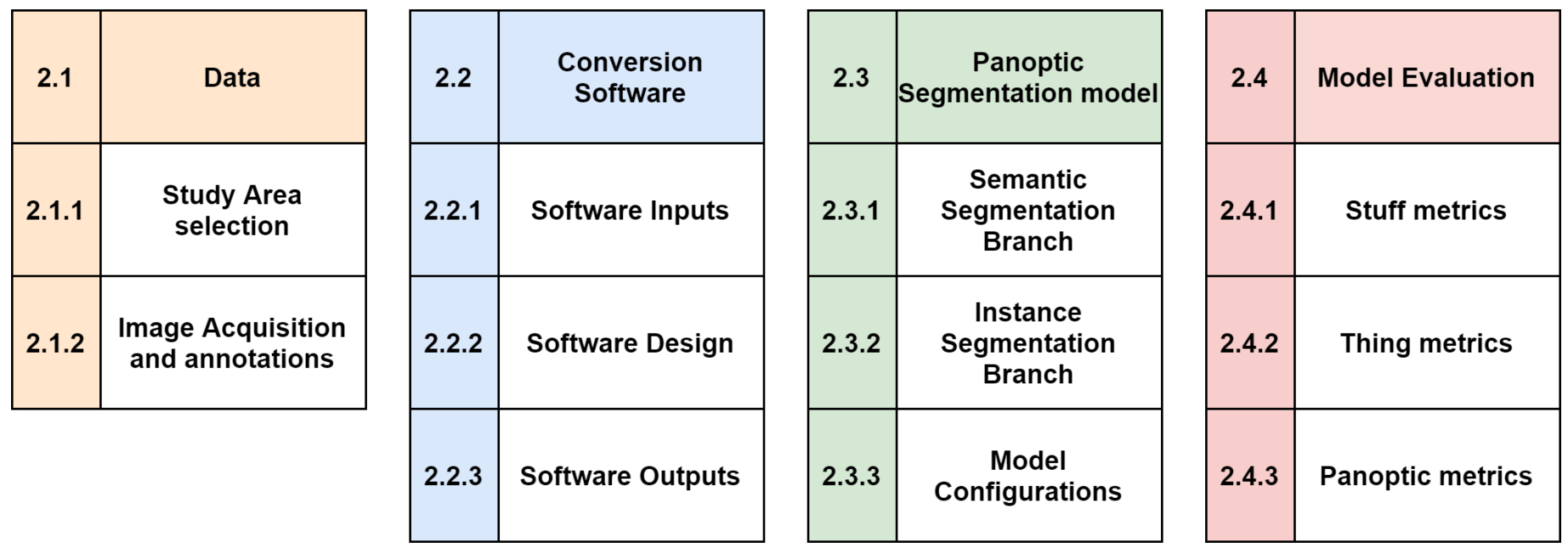
The present research had the following methodology (Figure 3): (Section 2.1) Data; (Section 2.2) Conversion Software; (Section 2.3) Panoptic Segmentation model; and (Section 2.4) Model evaluation.

2.1. Data

2.1.1. Study Area Selection

The study area was the city of Brasília (Figure 4), the capital of Brazil. Brasília was built and inaugurated in 1960 by President Juscelino Kubitschek to transfer the capital of Rio de Janeiro (in the coastal zone) to the country’s central region, aiming at modernization and integrated development of the nation. The capital’s original urban project was designed by the urban planner and architect Lúcio Costa, who modeled the city around Paranoá Lake with a top-view appearance of an airplane. The urban plan includes housing and commerce sectors around a series of parallel avenues 13 km long, containing zones dedicated to schools, medical services, shopping areas, and other community facilities. In 1988, United Nations Educational, Scientific and Cultural Organization (UNESCO) declared the city a World Heritage Site.

The city presents suitable characteristics for DL tasks: (1) it is one of the few planned cities in the world presenting well-organized patterns, which eases the process of understanding each class; (2) the buildings are not high, which reduces occlusion and shadows errors due to the photographing angle; (3) the city contains organized portions of houses, buildings, and commerce, facilitating the annotation procedure; and (4) it has many socio-economical differences in many parts of the city, bringing information that might be useful to many other cities in the world. The city setting is very suitable for developing panoptic segmentation applications since it presents countable objects (e.g., cars and houses) and amorphous targets (e.g., vegetation and lake) that wouldn’t be correctly represented by using only an instance or semantic segmentation approach.

2.1.2. Image Acquisition and Annotations

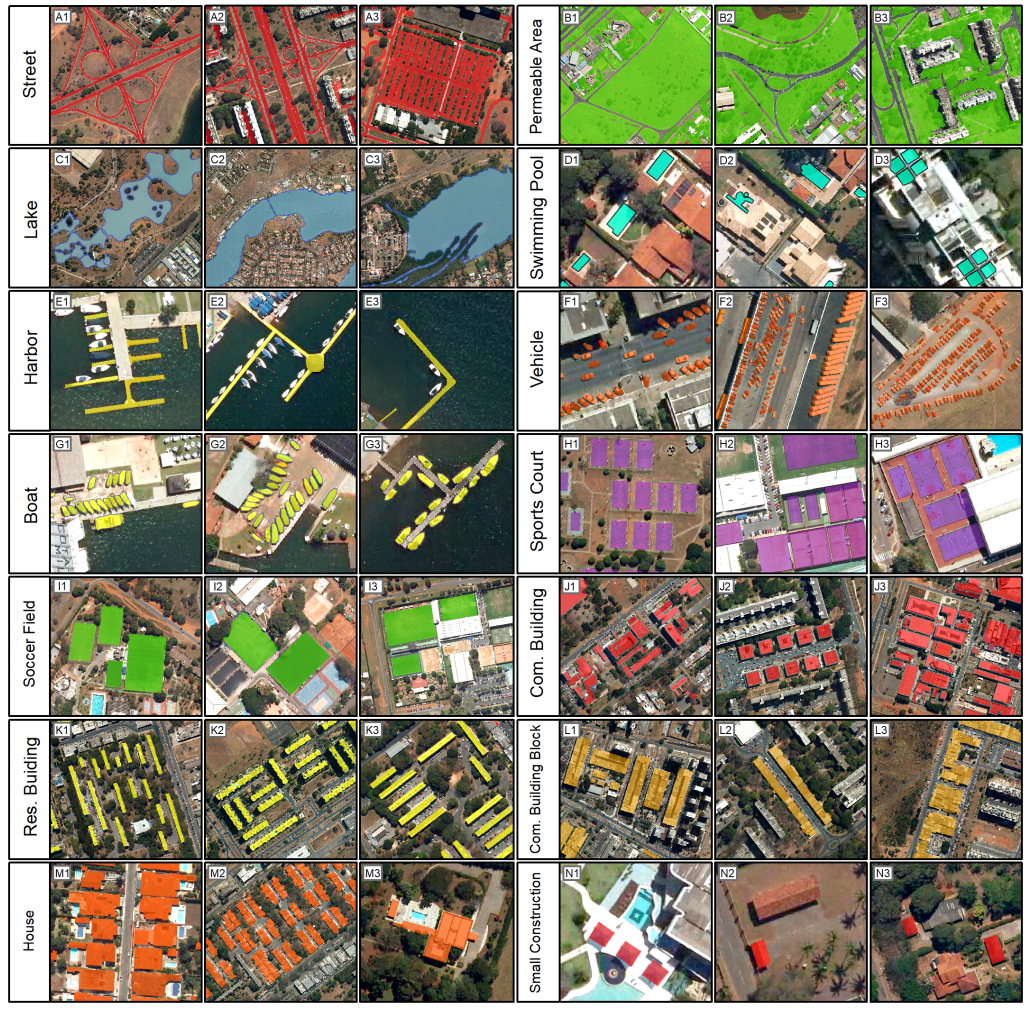
The aerial images present the RGB channels and spatial resolution of 0.24 meters over Brasilia cover an area of 79.40 km${}^2$, obtained by the Infraestrutura de Dados Espaciais do Distrito Federal (IDE/DF) (https://www.geoportal.seduh.df.gov.br/geoportal/, accessed on 25 January 2021). We made vectorized annotations using the ArcMap software considering fourteen urban classes (three “stuff” and eleven “thing” categories).

Table 1. Category, numeric label, thing/stuff, and number of instances used in the BSB Aerial Dataset. The number of polygons in the stuff categories receive the ’-’ symbol since it is not relevant.

Category	Label	Thing/Stuff	Polygons	Pixels	Annotation Pattern
Background	0	-	-	112,497,999	Unlabeled pixels
Street	1	Stuff	-	167,065,309	Visible asphalt areas
Permeable Area	2	Stuff	-	803,782,026	Natural soil and vegetation
Lake	3	Stuff	-	117,979,347	Natural water bodies
Swimming pool	4	Thing	4835	3,816,585	Swimming pool polygons
Harbor	5	Thing	121	214,970	Harbor polygons
Vehicle	6	Thing	84,675	11,458,709	Ground vehicle polygons
Boat	7	Thing	548	189,115	Boat polygons
Sports Court	8	Thing	613	3,899,848	Sports court polygons
Soccer Field	9	Thing	89	3,776,903	Soccer field polygons
Com. Buiding	10	Thing	3796	69,617,961	Commercial building rooftop polygons
Res. Buiding	11	Thing	1654	8,369,418	Residential building rooftop polygons
Com. Building Block	12	Thing	201	30,761,062	Commercial building block rooftops polygons
House	13	Thing	5061	42,528,071	House-like polygons with area > 80 m${}^2$
Small Construction	14	Thing	4552	2,543,032	House-like polygons with area < 80 m${}^2$

lists the panoptic categories with their annotation pattern, and Figure 5 shows three examples from each class. The vehicles presented the most polygons (84,675), whereas the soccer fields had only 89. This imbalance among the different categories is widespread due to the nature of the urban landscape, i.e., there are more cars than soccer fields in cities. The understanding of this imbalance is an essential topic for investigating DL algorithms in the city setting. Since there is high variability in the permeable areas, we made a more generalized class considering all types of natural lands and vegetation, being the class with the highest number of annotated pixels (803,782,026). Besides, the vehicle and boat polygons were obtained from de Carvalho et al. study [61].

2.2. Conversion Software

DL methods require extensive collections of annotated images with different object classes for training and evaluation. Different open-sourced annotation software has been proposed, containing high-efficiency tools for the creation of polygons and bounding boxes, such as Labelme [62,63], LabelImg (https://github.com/tzutalin/labelImg, accessed on 25 January 2021), Computer Vision Annotation Tool (CVAT) [64], RectLabel (https://rectlabel.com, accessed on 25 January 2021), Labelbox (https://labelbox.com), and Visual Object Tagging Tool (VoTT) (https://github.com/microsoft/VoTT, accessed on 25 January 2021).However, the elaboration of annotations in remote sensing differs from other computer vision procedures that use traditional photographic images (e.g., cellphone photos), containing some particularities, such as georeferencing, projection, multiple channels, and GeoTIFF files. Thus, there is a gap in specific annotation tools for remote sensing. In this context, a powerful solution for expanding the terrestrial truth database for DL is to take advantage of the extensive mapping information stored in a GIS database. Besides, GIS programs already have several editing, and manipulation tools developed and improved for geo-referenced data. Recently, a specific annotation tool for remote sensing is the LabelRS based on ArcGIS [65], considering semantic segmentation, object detection, and image classification. However, LabelRS is based on ArcPy scripts dependent on ArcGIS, not fully open-source, and does not operate with panoptic annotations.

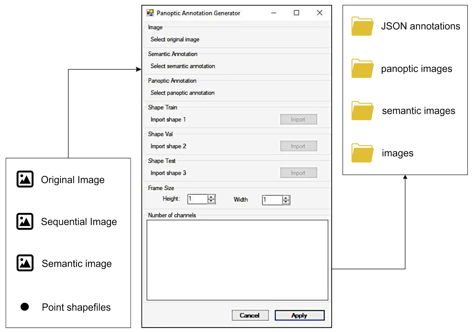
The present study develops a module within the Abilius software that converts GIS vector data into COCO-compatible annotations widely used in DL algorithms (Figure 6) (https://github.com/abilius-app/Panoptic-Generator, accessed on 25 January 2021). The proposed framework generates samples from vector data in shape format to JavaScript Object Notation (JSON) files in the COCO annotation format, considering the three main segmentation tasks (semantic, instance, and panoptic). The use of GIS databases provides a practical way to expand the free community-maintained datasets, minimizing the time-consuming and challenging process of manually generating large numbers of annotations for different classes of objects. The tool generates annotations for the three segmentation tasks in an end-to-end approach, in which the annotations are ready to use, requiring no intermediary process and reducing labor-intensive work. Besides, it is important to note that the conversion from raster data to polygons may bring imprecision at a pixel level since points represent the polygons. This imprecision can be minimized by changing the approximation function for the polygon generation. However, when considering more points for each polygon, the computational power increases, and those approximation differences are imperceptible for the spatial resolution of our images. Moreover, this tool was crucial to build the current dataset, but it also applies to other scenarios, since it just requires other researchers to follow our proposed pipeline using GIS software.

2.2.1. Software Inputs

To automatically obtain the semantic, instance, and panoptic annotations, we proposed a novel pipeline with four inputs (considering the georeferenced images in the same system): (a) the original image (Figure 7A); (b) semantic image (Figure 7B); (c) sequential ground truth image (Figure 7C) (each “thing” object has a different value), and (d) the point shapefiles (Figure 7D). The class-agnostic image is a traditional semantic segmentation ground truth, in which each class receives a unique label, easily achieved by converting from polygon to raster in GIS software. The sequential ground truth (which will become the panoptic images) requires a different value for each polygon that belongs to the “thing” categories. First, we grouped all the “stuff” classes since these classes do not need a unique identification. The subsequent “thing” classes receive a unique value to each polygon using sequential values in the attribute table. Moreover, the point shapefiles play a crucial role in generating the DL samples since it uses the point location as the centroid of the frame. Our proposed method using point shapefiles provides the following benefits: (a) more control over the selected data in each set; (b) allows augmenting the training data by choosing points close to each other; and (c) in large images, there are areas with much less relevance, and the user may choose more significant regions to generate the dataset. Apart from the inputs, the user may choose other parameters such as spectral bands and spatial dimensions. Our study used the RGB channels (other applications might require more channels or less depending on the sensor) and 512 × 512-pixel dimensions.

2.2.2. Software Design

Given the raw inputs, the software must crop tiles in the given point shapefile areas. For each point shapefile, it crops all input images considering the point as the centroid, meaning that if the user chooses a tile size of 512 × 512, the frame will present distance from the centroid of 256-pixels in the up, down, right, and left directions (resulting in a squared frame with 512 × 512 dimensions). Now, for each 512 × 512 tile, we must gather the image annotations semantic, instance, and panoptic segmentation tasks, given as follows:

• Semantic segmentation annotation: Pixel-wise classification of the entire image with the same spatial dimensions from the original image tiles. Usually, the background (i.e., unlabeled data) has a value of zero. Each class presents a unique value.
• Instance segmentation annotation: Each object requires a pixel-wise classification, bounding box, and class of each bounding box for each object. Since there is more information when compared to the semantic segmentation approach, most software adopts the COCO annotation format, e.g., Detectron2 [24]. For instance segmentation, the COCO annotation format uses a JSON file requiring for each object the: (a) identification, (b) image identification, (c) category identification (i.e., the label of the class), (d) segmentation (polygon coordinates), (e) area (total number of pixels), (f) bounding box (four coordinates) (https://cocodataset.org/#format-data, accessed on 25 January 2021).
• Panoptic segmentation annotation: The panoptic segmentation combines semantic and instance segmentation. It requires a folder with the semantic segmentation images in which all thing classes have zero value. Besides, it requires the instance segmentation JSON file and an additional panoptic segmentation JSON file. The panoptic JSON is very similar to the instance JSON, but considering an identifier named “isthing”, in which the “thing” category is one and “stuff” is zero.

The semantic segmentation data is the most straightforward, and its output cropped tiles are already in the format to apply a semantic segmentation model. Nevertheless, the semantic image plays a crucial role in the instance and panoptic JSON construction. The parameters designed to build the COCO annotation JSONS for instance and panoptic segmentation were the following:

• Image identification: Each cropped tile receives an ascending numeration. For example, there are 3000-point shapefiles in the training set, and the image identifications range from 1 to 3000.
• Segmentation: We used the OpenCV C++ library for obtaining all contours in the sequential image. The contour representation is in tuples (x and y). For each distinct value, the proposed software gathers all coordinates separately according to the COCO annotation specifications. The polygon information will only be stored in the instance segmentation JSON, but these coordinates will guide the subsequent bounding box process.
• Bounding box: Using the polygons obtained in the segmentation process enables the extraction of minimum and maximum points (in the horizontal and vertical directions). There are many possible ways to obtain the bounding box information using four coordinates. However, we used the top-left coordinates associated with the width and height.
• Area: We apply a loop to count the number of pixels of each different value on the sequential image.
• Category identification: This is where the segmentation image is so important. The sequential image does not contain any class information (only that each thing class has a different value). For each generated polygon, we extract the category value from the semantic image to use it as the category identification label.
• Object identification: This method is different for the instance and panoptic JSONS. In the instance JSON, the identification is a sequential ascending value (the last object in the last image will present the highest value, and the first object in the first image will present the lowest value), and it only considers the “thing” classes. In the panoptic JSON, the identification is the same as the object number in sequential order, and it considers “thing” and “stuff” classes.

Apart from these critical parameters, we did not consider the possibility of crowded objects (our data has all separate instances), so the “is_crowd” parameter is always zero. Moreover, the user must specify which classes are “stuff” or “things”. The sequential input data is an image with single-channel TIFF format transformed in our software to a three-channel PNG image compatible with Detectron2 software, converting from decimal number to base-256.

2.2.3. Software Outputs

The software outputs the images and annotations in a COCO dataset structure. The algorithm produces ten folders, an individual folder for annotations in JSON format and three folders for each set of samples (training, validation, and testing) referring to the original image, panoramic annotations, and semantic annotations. In the training-validation-test split, the training set usually presents most of the data for the purpose of learning the specific task. However, the training set alone is not sufficient to build an effective model since, in many situations, the model overfits the data after a certain point. Thus, the validation set allows tracking the trained model performance on new data while still tuning hyperparameters. The test set is an independent set to evaluate the performance.

Table 2. Data split on the three sets with their respective number of images and instances, in which all images present 512 × 512 × 3 dimensions.

Set	Number of Tiles	Number of Instances
Training	3000	102,971
Validation	200	9070
Test	200	7237

lists the number of tiles in each set and the total number of instances. Our proposed conversion software allows overlapping image tiles, which may be valuable in the training data functioning as a data augmentation method. However, this would lead to biased results if applied in the validation and testing sets. In this regard, we used the graphic Buffer analysis tool from the ArcMap software, considering the dimensions generating 512 × 512 squared buffers to verify that none of the sets were overlapping.

2.3. Panoptic Segmentation Model

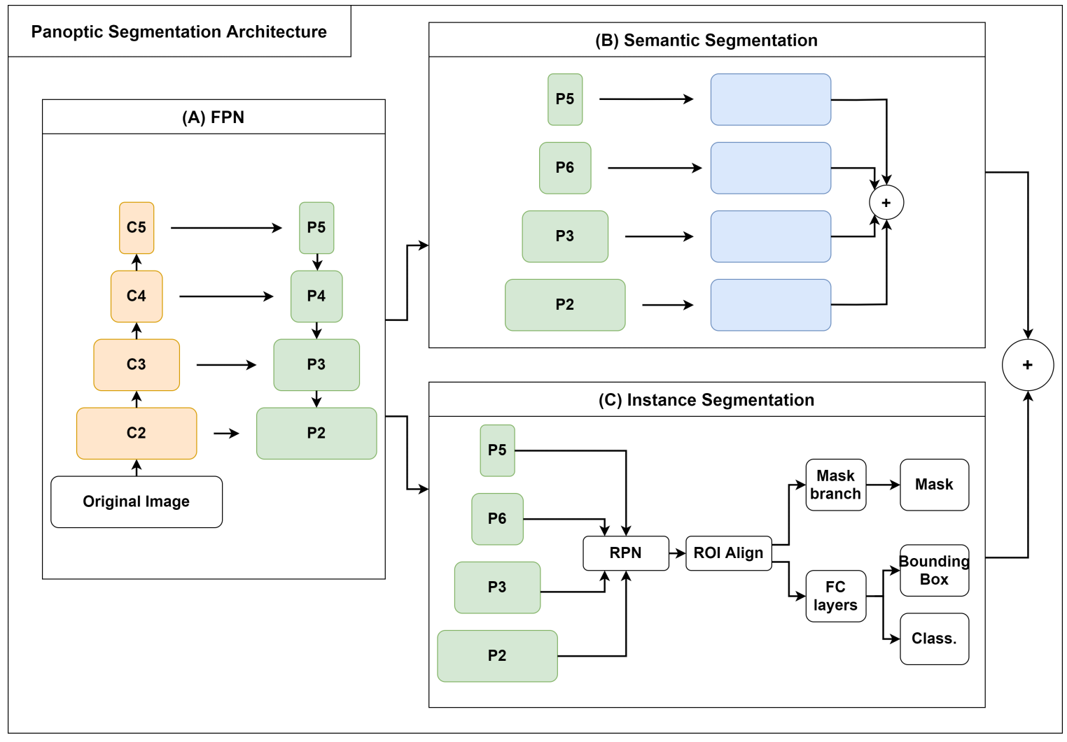
With the annotations in the correct format, the next step was to use panoptic segmentation DL models. Panoptic segmentation networks aim to combine the semantic and instance results using a simple heuristic method [23] (Figure 8). The model presents two branches: semantic segmentation (Figure 8B) and instance segmentation (Figure 8C). Figure 8 shows the Panoptic-FPN architecture, which use the FPN [66] as a common structure for both branches (Figure 8A. Besides, we considered two backbones, the ResNet-50 and ResNet-101.

2.3.1. Semantic Segmentation Module

Semantic segmentation models are the most used among the remote sensing community, mainly because of the good results and simplicity of models and annotation formats. There are a wide variety of architectures such as the U-net [67], Fully Convolutional Networks (FCN) [68], DeepLab [53]. The semantic segmentation using the FPN presents some differences when compared to traditional encoder-decoder structures. FPN predictions with different scales (P2, P3, P4, P5) are resized to the input image spatial resolution by applying bilinear upsampling, in which the sampling rate is different for each prediction to obtain the same dimensions as shown in Figure 8B. The elements present in the “things” category all receive the same label (avoiding problems with the predictions from the instance segmentation branch).

2.3.2. Instance Segmentation Module

Instance segmentation had a significant breakthrough with the Mask-RCNN [16]. This method relies on the extension of Faster-RCNN [69], a detector with two stages: (a) Region Proposal Network (RPN); and (b) box regression and classification for each Region of Interest (ROI) from the RPN. However, aiming to perform pixel-wise segmentation, the Mask-RCNN added a segmentation branch on top of the Faster-RCNN architecture. First, the method applies the RPN on top of different scale predictions (e.g., P2, P3, P4, P5) and proposes several anchor boxes in more susceptible regions. Then, the ROI align procedure standardizes each bounding box dimension (avoiding quantization problems) as shown in Figure 8C. The last step considers a binary segmentation mask for each object alongside the bounding box with its respective classification.

2.3.3. Model Configurations

The loss function for the Panoptic-FPN model is the combination of the semantic and instance segmentation losses. The instance segmentation encompasses the bounding box regression, classification, and mask losses. The semantic segmentation uses a traditional cross-entropy loss among the “stuff” categories and a class considering all “thing” categories together.

Regarding the model hyperparameters, we used: (a) stochastic gradient descent (SGD) optimizer, (b) learning rate of 0.0005, (c) 150,000 iterations, (d) five anchor boxes (with sizes 32, 64, 128, 256, and 512), (e) three aspect ratios (0.5, 1, 2), (f) one image per batch. Besides, we trained the model using ImageNet pre-trained weights and unfreezing all layers. Moreover, we evaluated the metrics on the validation set with a period of 1000 iterations and saved the final model with the highest PQ metric. To avoid overfitting and increase performance (mainly on the small objects), we used three augmentation strategies: (a) random vertical flip (probability chance of 50%), (b) random horizontal flip (probability chance of 50%), and (c) resize shortest edge with 640, 672, 704, 736, 768, and 800 possible sizes. The data processing used a computer containing an Intel i7 core and NVIDIA 2080 GPU with 11GB RAM.

2.4. Model Evaluation

In supervised learning tasks, the accuracy analysis compares the predicted results and the ground truth data. Each task has different ground truth data and, therefore, different evaluation metrics. However, the confusion matrix is a common structure for all tasks, yielding four possible results: true positives (TP), true negatives (TN), false positives (FP), and false negatives (FN). Section 2.4.1, Section 2.4.2, Section 2.4.3 explain the semantic, instance, and panoptic segmentation metrics, respectively.

2.4.1. Stuff Evaluation

For semantic segmentation tasks, the confusion matrix analysis is per pixel. The most straightforward metric is the pixel accuracy (pAcc):

$$\mathrm{p}\mathrm{A}\mathrm{c}\mathrm{c}=\frac{\mathrm{T}\mathrm{P}+\mathrm{T}\mathrm{N}}{\mathrm{T}\mathrm{P}+\mathrm{T}\mathrm{N}+\mathrm{F}\mathrm{P}+\mathrm{F}\mathrm{N}}$$

(1)

However, in many cases, the classes are imbalanced, bringing imprecise results. The mean pixel accuracy (mAcc) takes into consideration the number of pixels belonging to each class, performing a weighted average.

Apart from PA, the intersection over union (IoU) is the primary metric for many semantic segmentation studies, mainly because it penalizes the algorithm for FP and FN errors:

$$\mathrm{I}\mathrm{o}\mathrm{U}=\frac{|A\cap B|}{|A\cup B|}=\frac{\mathrm{T}\mathrm{P}}{\mathrm{T}\mathrm{P}+\mathrm{F}\mathrm{P}+\mathrm{F}\mathrm{N}}$$

(2)

In which: $A\cap B$: the area of intersection; $A\cup B$: the area of union.

For a more general understanding of this metric, we may use the mean IoU (mIoU), which is the average IoU of all categories or the frequency weighted IoU (fwIoU) which is the weighted average of each IoU considering the frequency of each class.

2.4.2. Thing Evaluation

Instance segmentation metrics take into consideration both the bounding box predictions and the mask quality. The most common approach to instance segmentation problems uses standard COCO metrics [16,27,35,70,71]. The primary metric in evaluation is the average precision (AP) [20], also known as the area under the precision-recall curve:

$$\mathrm{A}\mathrm{P}={\int }_0^1\mathrm{Precision}\left(\mathrm{Recall}\right)\mathrm{dRecall},$$

(3)

in which:

$$\mathrm{Precision}=\frac{\mathrm{T}\mathrm{P}}{\mathrm{T}\mathrm{P}+\mathrm{F}\mathrm{P}}$$

(4)

$$\mathrm{Recall}=\frac{\mathrm{T}\mathrm{P}}{\mathrm{T}\mathrm{P}+\mathrm{F}\mathrm{N}}$$

(5)

Moreover, the COCO AP metrics consider different IoU thresholds from 0.5 to 0.95 with 0.05 steps, which is useful to measure the quality of the bounding boxes compared to the original image. The secondary metrics consider specific IoU thresholds: AP${}_{50}$ and AP${}_{75}$, which use IoU values of 0.5 and 0.75, respectively. Besides, the evaluation considers different sized objects (AP${}_S$, AP${}_M$, and AP${}_L$): (1) small objects (<32${}^2$ pixels); (2) medium objects (32${}^2$ pixels < area < 96${}^2$ pixels); and (3) large objects (>96${}^2$ pixels).

2.4.3. Panoptic Evaluation

The Panoptic Quality (PQ) is the primary metric for evaluating the Panoptic Segmentation task [23,26,27], and it is the current metric for the COCO panoptic task challenge, being defined by:

$$\mathrm{P}\mathrm{Q}=\frac{{\sum }_{\left(\mathrm{p},\mathrm{g}\right)\in \mathrm{T}\mathrm{P}}\mathrm{I}\mathrm{o}\mathrm{U}\left(pred,\mathrm{G}\mathrm{T}\right)}{\left|\mathrm{T}\mathrm{P}\right|+\frac{1}{2}\left|\mathrm{F}\mathrm{P}\right|+\frac{1}{2}\left|\mathrm{F}\mathrm{N}\right|}$$

(6)

In which p is the DL prediction, and g is the ground truth. The expression above is the multiplication of two metrics, the Segmentation Quality (SQ) and Recognition Quality (RQ), expressed by:

$$\mathrm{S}\mathrm{Q}=\frac{{\sum }_{\left(\mathrm{p},\mathrm{g}\right)\in \mathrm{T}\mathrm{P}}\mathrm{I}\mathrm{o}\mathrm{U}(pred,\mathrm{G}\mathrm{T})}{\left|\mathrm{T}\mathrm{P}\right|}$$

(7)

$$\mathrm{R}\mathrm{Q}=\frac{\mathrm{T}\mathrm{P}}{\left|\mathrm{T}\mathrm{P}\right|+\frac{1}{2}\left|\mathrm{F}\mathrm{P}\right|+\frac{1}{2}\left|\mathrm{F}\mathrm{N}\right|}$$

(8)

3. Results

3.1. Metrics

The metrics section presents (Section 3.1.1) semantic segmentation metrics, (Section 3.1.2) instance segmentation metrics, and (Section 3.1.3) panoptic segmentation metrics. The semantic segmentation metrics are related to the “stuff” classes in a per-pixel analysis. The instance segmentation classes relate to the “thing” classes using traditional object detection metrics, such as the AP. The panoptic segmentation metrics englobes both types of features.

3.1.1. Semantic Segmentation Results

Table 3. Mean Intersection over Union (mIoU), frequency weighted (fwIoU), mean accuracy (mAcc), and pixel accuracy (pAcc) results for semantic segmentation in the BSB Aerial Dataset validation and test sets.

Backbone	mIoU	fwIoU	mAcc	pAcc
Validation Set
R50	92.129	92.865	95.643	96.271
R101	92.643	93.241	95.769	96.485
Difference	0.514	0.376	0.126	0.214
Test Set
R50	92.381	93.404	95.772	96.573
R101	93.865	94.472	96.339	97.148
Difference	1.484	1.068	0.567	0.575

lists the general metrics for the three “stuff” categories (street, permeable area, and lake), considering the mIoU, fwIoU, mAcc, and pAcc for the Panoptic-FPN model with the ResNet-50 and ResNet-101 backbones. The validation and test results were very similar, in which the R101 backbone presented slightly better results among all metrics. In the validation and test sets, the metric with the most considerable difference between the ResNet-50 and ResNet-101 backbones was the IoU (0.514 and 1.484 difference in the validation and test set, respectively).

Table 4. Segmentation metrics (Intersection over Union (IoU) and Accuracy (Acc)) for each “stuff” classes in the BSB Aerial dataset validation and test sets considering the ResNet101 (R101), ResNet50 (R50) backbones, and their difference (R101–R50).

Category	R101		R50		Difference
	IoU	Acc	IoU	Acc	IoU	Acc
Validation Set
All things	89.962	95.060	89.402	94.882	0.56	0.178
Street	88.079	91.773	86.933	91.799	1.146	−0.026
Permeable Area	95.384	98.090	95.286	97.786	0.098	0.304
Lake	97.148	98.153	96.993	98.105	0.155	0.048
Test Set
All things	90.718	94.563	89.142	93.041	1.576	1.522
Street	90.607	93.600	89.129	93.844	1.478	−0.244
Permeable Area	96.275	98.775	95.559	98.120	0.716	0.655
Lake	97.859	98.459	95.665	98.013	2.194	0.446

lists the accuracy results of each “stuff” class for the validation and test sets. In addition to the three stuff classes (lake, permeable area, and street), the analysis creates another class merging the “thing” classes (we defined it as “all things”). Some samples have a single-class predominance, such as lake and permeable area, increasing the accuracy metric due to the high proportion of correctly classified pixels. The “lake” class presented the highest IoU for the validation (97.1%) and test (97.8%) sets, mainly because it presents very distinct characteristics from all other classes in the dataset. The permeable area achieves a slightly lower accuracy (IoU of 95.384 for validation and 96.275 for the test) than the lake class because it encompasses many different intraclass features (e.g., trees, grass, earth, sand). The “street” class, widely studied in remote sensing, presented an IoU of 88% and 90% for validation and test. These IoU values are significant considering the difficulty of street mapping even by visual interpretation due to the high interference of overlapping objects (e.g., cars, permeable areas, undefined elements) and the challenges with shaded areas.

The R101 backbone presented better IoU results for all categories. The most significant difference was the street category in the validation set (1.146) and the lake in the test set (2.194). The R50 backbone presented a higher value for the street class in the validation (0.026) and test sets (0.244). Since the balancing of the classes is not even, the IoU provides more insightful results when compared to the accuracy.

3.1.2. Instance Segmentation Results

Table 5. COCO metrics for the “thing” categories in the BSB Aerial Dataset validation set considering two backbones (ResNet-101 (R101) and ResNet-50 (R50)) and their difference (R101–R50).

Backbone	Type	AP	${\mathbf{AP}}_{50}$	${\mathbf{AP}}_{75}$	${\mathbf{AP}}_{\mathit{S}}$	${\mathbf{AP}}_{\mathit{M}}$	${\mathbf{AP}}_{\mathit{L}}$
Validation Set
R101	Box	47.266	69.351	50.206	26.154	51.667	55.680
	Mask	45.379	68.331	50.917	24.064	49.490	57.882
R50	Box	45.855	68.258	51.351	25.806	49.732	48.678
	Mask	42.850	68.553	48.863	21.213	47.686	47.040
Difference	Box	1.411	1.093	−1.145	0.348	1.935	6.993
	Mask	2.529	2.778	2.054	2.851	1.804	10.842
Test Set
R101	Box	47.691	67.096	52.552	28.920	49.795	57.446
	Mask	44.211	65.271	49.394	25.016	49.377	58.311
R50	Box	44.642	64.306	50.727	28.636	49.881	53.298
	Mask	41.933	62.821	47.640	23.631	50.027	52.204
Difference	Box	3.049	2.790	1.825	0.284	−0.086	4.148
	Mask	2.278	2.450	1.754	1.385	−0.650	6.107

lists the results for the standard COCO metrics (AP, AP${}_{50}$, AP${}_{75}$, AP${}_S$, AP${}_M$, and AP${}_L$) for the “thing” classes, considering the bounding box (Box) and segmentation mask (mask), from the two backbones (ResNet-101 (R101) and ResNet-50 (R50)). The validation and test results were very similar to those occurring in the “stuff” classes. However, the primary metric (AP) differences among the two backbones (R101–R50) were more considerable in the test set regarding the box metrics, with a difference of nearly 1.6%. The R101 backbone had higher values in almost all derived metrics, except for the AP75 box metric in the validation set and the APmedium in the test set.

Although the overall metrics showed better performance for the R101 backbone, the analysis by class presents some classes with slightly better results for the R50 backbone (

Table 6. AP metrics for bounding box and mask per category considering the “thing” classes in the BSB Aerial Dataset validation set for the ResNet101 (R101) and ResNet50 (R50) backbones and their difference (R101-R50).

Category	R101		R50		Difference
	Box AP	Mask AP	Box AP	Mask AP	Box AP	Mask AP
Validation Set
Swimming pool	55.495	53.857	53.121	51.974	2.374	1.883
Harbor	37.137	21.079	39.415	24.300	−2.278	−3.221
Vehicle	55.616	56.573	54.568	55.893	1.048	0.680
Boat	30.582	36.216	35.329	37.265	−4.747	−1.049
Sports court	56.681	55.193	46.906	42.494	9.775	12.699
Soccer field	34.866	39.569	39.619	41.767	−4.753	−2.198
Com. building	32.114	31.799	28.592	28.471	3.522	3.328
Com. building block	66.283	63.192	52.149	47.606	14.134	15.586
Residential building	67.046	57.615	63.512	54.312	3.534	3.303
House	57.555	56.697	59.907	57.470	−2.352	−0.773
Small construction	26.550	27.381	31.284	29.800	−4.734	−2.419
Test Set
Swimming pool	53.561	50.044	51.546	50.520	2.015	−0.476
Harbor	42.429	22.837	31.409	17.270	11.02	5.567
Vehicle	56.371	57.689	55.695	57.311	0.676	0.378
Boat	26.190	31.210	30.698	34.875	−4.508	−3.665
Sports court	46.018	45.515	40.566	40.672	5.452	4.843
Soccer field	46.279	45.831	36.832	33.886	9.447	11.945
Com. building	42.516	37.709	41.145	40.265	1.371	−2.556
Com. building block	70.971	67.465	69.341	63.679	1.63	3.786
Residential building	54.829	47.397	51.774	44.640	3.055	2.757
House	62.395	59.886	57.861	58.396	4.534	1.490
Small construction	26.046	20.740	24.202	19.746	1.844	0.994

). In the validation set, five of the eleven classes had higher values in the ResNet-50 backbone (harbor, boat, soccer field, house, and small construction). This effect was less frequent in the test set, showing only the boat class with superiority of the ResNet-50 backbone in the box metric and three classes (swimming pool, boat, and commercial building) in the mask metric.

3.1.3. Panoptic Segmentation Results

Table 7. COCO metrics for panoptic segmentation in the BSB Aerial Dataset validation and test sets considering the Panoptic Quality (PQ), Segmentation Quality (SQ), and Recognition Quality (RQ).

Backbone	Type	PQ	SQ	RQ
Validation Set
R101	All	65.296	85.104	76.229
	Things	59.783	82.876	71.948
	Stuff	85.508	93.272	91.925
R50	All	63.829	84.886	74.550
	Things	57.958	82.777	69.674
	Stuff	85.354	92.617	92.432
Difference	All	1.467	0.218	1.679
	Things	1.825	0.099	2.274
	Stuff	0.154	0.655	−0.507
Test Set
R101	All	64.979	85.378	75.474
	Things	58.354	83.171	69.997
	Stuff	89.272	93.468	95.558
R50	All	62.230	85.315	72.179
	Things	55.239	83.344	65.956
	Stuff	87.864	92.540	94.998
Difference	All	2.749	0.063	3.295
	Things	3.115	−0.173	4.041
	Stuff	1.408	0.928	0.560

lists the results for the panoptic segmentation metrics (PQ, SQ, and RQ), which are the main metrics for evaluating this task. In hand with the previous “stuff” and “thing” results, the ResNet-101 backbone presented the best metrics in most cases, except for the RQ${}_{stuff}$ in the validation set and the SQ${}_{things}$ in the test set. Overall, the main metric for analysis (PQ) had nearly a 2% difference among the backbones. The low discrepancies among the different architectures suggest that in situations with lower computational power, the usage of a lighter backbone still presents close enough results.

3.2. Visual Results

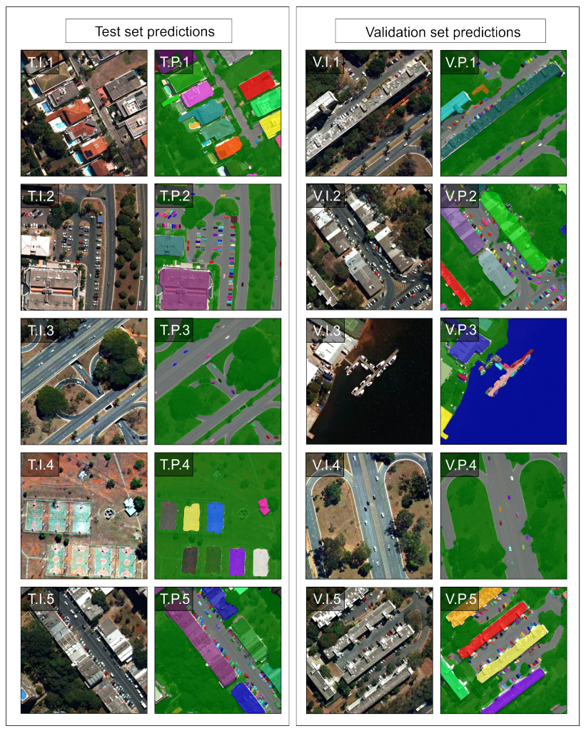
Figure 9 shows five test and validation samples, including the original images and predictions from the Panoptic-FPN model using the ResNet-101 backbone. The results demonstrate a coherent urban landscape segmentation, visually integrating countable objects (things) and amorphous regions (things) in an enriching perspective toward real-world representation. Among the ten image pairs, there is at least one representation of each of the fourteen classes. As shown in the metrics section, the results present no evident discrepancies in the validation and testing data, demonstrating very similar visual results in both sets. The segmented images show the high ability to visually separate the different instances, even in crowded situations like cars in parking lots. Furthermore, the “stuff” classes are very well delineated, showing little confusion among the street, permeable areas, and lake classes. The set of established classes allows a good representation of the urban landscape elements, even considering some class simplifications. Therefore, panoptic segmentation congregates multiple competencies in computer vision for the satellite imagery interpretation in a single structure.

4. Discussion

The panoptic segmentation task imposes new challenges in the formulation of algorithms and database structures, covering particularities of both object detection and semantic segmentation. Therefore, panoptic segmentation establishes a unified image segmentation approach, which changes digital image processing and requires new annotation tools and extensive and adapted datasets. In this context, this research innovates by developing a panoptic data annotation tool, establishing a panoptic remote sensing dataset, and being one of the first evaluations of the use of panoptic segmentation in urban aerial images.

4.1. Annotation Tools for Remote Sensing

Many software annotation tools are available online, e.g., LabelMe [62]. Nevertheless, those tools have problems with satellite image data because of large sizes and other singularities that are uncommon in the traditional computer vision tasks: (a) image format (i.e., satellite imagery is often in GeoTIFF, whereas traditional computer vision uses PNG or JPEG images), (b) georeferencing, and (c) compatibility with polygon GIS data. The remote sensing field made use of GIS software long before the rise of DL. With that said, there are extensive collections of GIS data (urban, agriculture, change detection) that other researchers could apply DL models. However, vector-based GIS data requires modifications to use DL models. Thus, we proposed a conversion tool from GIS data that automatically crops image tiles with their corresponding polygon vector data stored in shapefile format to panoptic, instance, and semantic annotations. The proposed tool is open access and works independently, without the need to use proprietary programs such as LabelRS developed by ArcPy and dependent on ArcGis [65]. Besides, our proposed pipeline and software enable the users to choose many samples for training, validation, and testing in strategic areas using point shapefiles. This method of choosing samples presents a huge benefit compared to methods such as sliding windows for image generation. Finally, our software enables the generation of the three segmentation tasks (instance, semantic, and panoptic), allowing other researchers to exploit the field of desire.

4.2. Datasets

Most transfer learning applications use trained models from extensive databases such as the COCO dataset. Nevertheless, remote sensing images present characteristics that may not yield the most optimal results using traditional images. These images contain diverse targets and landscapes, with different geometric shapes, patterns, and textural attributes, representing a challenge for automatic interpretation. Therefore, the effectiveness of training and testing depends on accurately annotated ground truth datasets, which requires much effort into building large remote sensing databases with a significant variety of classes. Furthermore, the availability of open access encourages new methods and applications, as seen in other computer vision tasks.

Long et al. [72] performed a complete review of remote sensing image datasets for DL methods, including tasks of scene classification, object detection, semantic segmentation, and change detection. In this recent review, there is no database for panoptic segmentation, which demonstrates a knowledge gap. Most datasets consider limited semantic categories or target a specific element, such as building [37,73,74], vehicle [75,76,77], ship [78,79,80], road [81,82], among others. Regarding available remote sensing datasets for various urban categories, one of the main is the iSAID [83], with 2806 aerial images distributed in 15 different classes, for instance segmentation and object detection tasks.

The scarcity of remote sensing databases with all cityscape elements makes mapping difficult due to highly complex classes, numerous instances, and mainly intraclass and interclass elements commonly neglected. Adopting the panoptic approach allows us to relate the content of interest and the surrounding environment, which is still little explored. Therefore, organizing large datasets into panoptic categories is a key alternative to mapping complex environments such as urban systems that are not reached even with enriched semantic categories.

The proposed BSB Aerial Dataset contains 3400 images (3000 for training, 200 for validation, and 200 for testing) with 512 × 512 dimensions containing fourteen common urban classes. This dataset simplified some urban classes, such as sports courts instead of tennis courts, soccer fields, and basketball courts. Moreover, our dataset considers three “stuff” classes, widely represented in the urban setting, such as roads. The availability of data and the need for periodic mapping of urban infrastructure by the government allows for the constant improvement of this database. Besides, the dataset aims to trigger other researchers to exploit this task thoroughly.

4.3. Difficulties in the Urban Setting

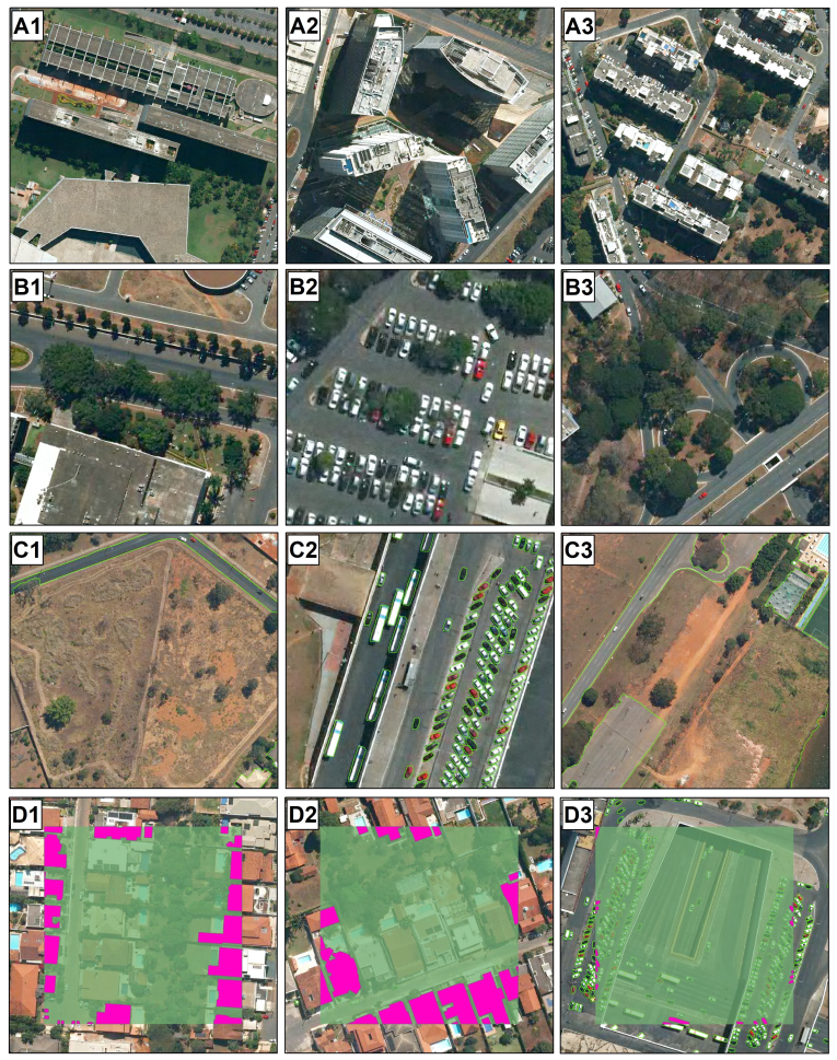
Although this study shows a promising field in remote sensing with a good capability of identifying “thing” and “stuff” categories simultaneously, we observed four main difficulties in image annotation and possible results in the urban setting (Figure 10): (1) shadows, (2) occlusion objects, (3) class categorization, and (4) edge problem on the image tiles. Shadows entirely or partially obstruct the light and occur under diverse conditions from the different objects (e.g., cloud, building, mountain, and trees), requiring well-established ground rules to obtain consistent annotations. Therefore, the shadow presence is a source of confusion and misclassification, reducing image quality for visual interpretation and segmentation and, consequently, negatively impacting the accuracy metrics [84] (Figure 10(A1–A3)). Specifically, urban landscapes have a high proportion of areas covered by shadows due to the high density of tall objects. Therefore, urban zones aggravate the interference of shadows, causing semantic ambiguity and incorrect labeling, which is a challenge in remote sensing studies [72,85]. DL methods tend to minimize shading effects, but errors occur in very low light locations. Another fundamental problem in computer vision is the occlusion that impedes object recognition in satellite images. Commonly, there are many object occlusions in the urban landscape, such as vehicles partially covered by trees and buildings, making their identification difficult even for humans (Figure 10(B1–B3)).

Like the occlusion problem, the objects that rely on the tile edges may present an insufficient representation. In monothematic studies, the authors may design the dataset to avoid this problem. However, for the panoptic segmentation task, which aims for an entire scene pixel-wise classification, some objects will be partial representation no matter how large we choose the image tile (Figure 10(D1–D3)). Our proposed annotation tool enables the authors to select each tile’s exact point, which gives data generation autonomy to avoid very few representations (even though the problem will still be present). By choosing large image tiles, the percentual representation of edge objects will be lower and tends to have a smaller impact on the model and accuracy metrics but increasing the image tile also requires more computational power.

Finally, the improvement of urban classes in the database is ongoing work. This research sought to establish general and representative classes, but the advent of new categories will allow for more detailed analysis according to research interests. For example, our vehicle class encompasses buses, small cars, and trucks, and our permeable area class contains bare ground, grass, and trees as shown in Figure 10(C1–C3).

4.4. Panoptic Segmentation Task

The remote sensing field is prone to using panoptic segmentation, mainly when referring to satellite and aerial images that do not require real-time processing. Most images have a frequency of at least days apart from each other, making some widely studied metrics such as inference time much less relevant. In remote sensing, the more information we can get simultaneously, the better. However, panoptic segmentation presents some non-trivial data generation mechanisms that require information for both instance and semantic segmentation. Besides, the existing panoptic segmentation studies that develop novel remote sensing datasets do not fully embrace the “stuff” classes [32,33].

The panoptic segmentation may represent a breakthrough in the remote sensing field for the ability to gather countable objects and background elements using a single framework, surpassing some difficulties of semantic and instance segmentation. Nonetheless, the data generation process and configuration of the models are much less straightforward than other methods, highlighting the importance of shortening this gap.

4.5. Limitations and Future Work

The high diversity of properties in remote sensing images (different spatial, spectral, and temporal resolutions) and the different landscapes of the Earth’s surface make it a challenge to formulate a generalized DL dataset. In this sense, our proposed annotation tool is suitable for creating datasets considering different image types. Future research on panoptic segmentation in remote sensing should progress to include images from various sensors, allowing faster advances in its application.

Furthermore, an important advance for panoptic segmentation is to include occlusion scenarios. Currently, the panoptic segmentation and its subsequent metrics (PQ, SQ, and RQ) require no overlapping segments, i.e., it considers only the visible pixels of the images. The usage of top-view images is very susceptible to classifying non-visible areas (occluded targets). Those changes would require adaptations in the models and metrics.

Practical remote sensing applications also require mechanisms for classifying large regions. Those methods usually use sliding windows, which have different peculiarities for pixel-based (e.g., semantic segmentation) and box-based methods (e.g., instance segmentation). The semantic segmentation approach use sliding windows with overlapping pixels, in which overlapped pixels are averaged. This averaging procedure attenuates the borders and enhances the metrics [86,87,88]. The instance segmentation proposals use sliding windows with a half-frame stride value, which allows identifying the elements as a whole and eliminating partial predictions [28,89]. There is no specific method for using a panoptic segmentation framework using sliding windows.

5. Conclusions

The application of panoptic, instance and semantic segmentation often depends on the desired outcome of a research or industry application. Nevertheless, a research gap in the remote sensing community is the lack of studies addressing panoptic segmentation, one of the most powerful techniques. The present research proposed an effective solution for using this unexplored and powerful method in remote sensing by: (a) providing a large dataset (BSB aerial dataset) containing 3400 images with 512 × 512 pixel dimensions in the COCO annotation format and fourteen classes (eleven “thing” and three “stuff” categories), being suitable for testing new DL models, (b) providing a novel pipeline and software for easily generating panoptic segmentation datasets in a format that is compatible with state-of-the-art software (e.g., Detectron2), and (c) leveraging and modifying structures in the DL models for remote sensing applicability, and (d) making a complete analysis of different metrics and evaluating difficulties of this task in the urban setting. One of the main challenges for preparing a panoptic segmentation model is the image format, which is still not well documented. Thus, we proposed an automatic converter from GIS data to panoptic, instance, and semantic segmentation formats. GIS data was widespread even before the DL rise, and the number of datasets that could benefit from our method is enormous. Besides, our tool allows the users to choose the exact points in large images to generate the DL samples using point shapefiles, which brings more autonomy to the studies and allows better data choosing. We believe that this work may increase other studies on the panoptic segmentation task with the BSB Aerial Dataset and the annotation tool and the baselines comparisons using well-documented software (Detectron2). Moreover, we evaluated the Panoptic-FPN model using two backbones (ResNet-101 and ResNet-50), showing promising metrics for this method’s usage in the urban setting. Therefore, this research shows an effective annotation tool, a large dataset for multiple tasks, and their application on some non-trivial models. Regarding future studies, we discussed three major problems to be addressed: (1) augmenting the dataset with images with different spectral bands and spatial resolution, (2) expand the panoptic idea for occlusion scenarios in remote sensing, and (3) adapt methods for classifying large images.

References

1. Ma, L.; Liu, Y.; Zhang, X.; Ye, Y.; Yin, G.; Johnson, B.A. Deep learning in remote sensing applications: A meta-analysis and review. ISPRS J. Photogramm. Remote Sens. 2019, 152, 166–177. [Google Scholar] [CrossRef]
2. Maxwell, A.E.; Warner, T.A.; Fang, F. Implementation of machine-learning classification in remote sensing: An applied review. Int. J. Remote Sens. 2018, 39, 2784–2817. [Google Scholar] [CrossRef] [Green Version]
3. Shao, Y.; Lunetta, R.S. Comparison of support vector machine, neural network, and CART algorithms for the land-cover classification using limited training data points. ISPRS J. Photogramm. Remote Sens. 2012, 70, 78–87. [Google Scholar] [CrossRef]
4. Lecun, Y.; Bengio, Y.; Hinton, G. Deep learning. Nature 2015, 521, 436–444. [Google Scholar] [CrossRef] [PubMed]
5. Nogueira, K.; Penatti, O.A.; dos Santos, J.A. Towards better exploiting convolutional neural networks for remote sensing scene classification. Pattern Recognit. 2017, 61, 539–556. [Google Scholar] [CrossRef] [Green Version]
6. Simonyan, K.; Zisserman, A. Very Deep Convolutional Networks for Large-Scale Image Recognition. arXiv 2015, arXiv:1409.1556. [Google Scholar]
7. He, K.; Zhang, X.; Ren, S.; Sun, J. Deep Residual Learning for Image Recognition; IEEE: Las Vegas, NV, USA, 2016; Volume 45, pp. 770–778. [Google Scholar] [CrossRef] [Green Version]
8. Krizhevsky, A.; Sutskever, I.; Hinton, G.E. ImageNet classification with deep convolutional neural networks. Commun. ACM 2017, 60, 84–90. [Google Scholar] [CrossRef]
9. Xie, S.; Girshick, R.; Dollar, P.; Tu, Z.; He, K. Aggregated Residual Transformations for Deep Neural Networks; IEEE: Honolulu, HI, USA, 2017; pp. 5987–5995. [Google Scholar] [CrossRef] [Green Version]
10. Tan, M.; Le, Q. Efficientnet: Rethinking model scaling for convolutional neural networks. In Proceedings of the International Conference on Machine Learning, Long Beach, CA, USA, 9–15 June 2019; pp. 6105–6114. [Google Scholar]
11. Dhillon, A.; Verma, G.K. Convolutional neural network: A review of models, methodologies and applications to object detection. Prog. Artif. Intell. 2020, 9, 85–112. [Google Scholar] [CrossRef]
12. Hoeser, T.; Bachofer, F.; Kuenzer, C. Object detection and image segmentation with deep learning on earth observation data: A review—Part II: Applications. Remote Sens. 2020, 12, 3053. [Google Scholar] [CrossRef]
13. Voulodimos, A.; Doulamis, N.; Doulamis, A.; Protopapadakis, E. Deep Learning for Computer Vision: A Brief Review. Comput. Intell. Neurosci. 2018, 2018, 1–13. [Google Scholar] [CrossRef]
14. Yuan, X.; Shi, J.; Gu, L. A review of deep learning methods for semantic segmentation of remote sensing imagery. Expert Syst. Appl. 2021, 169, 114417. [Google Scholar] [CrossRef]
15. Singh, R.; Rani, R. Semantic Segmentation using Deep Convolutional Neural Network: A Review. SSRN Electron. J. 2020, 1–8. [Google Scholar] [CrossRef]
16. He, K.; Gkioxari, G.; Dollar, P.; Girshick, R. Mask R-CNN. IEEE Trans. Pattern Anal. Mach. Intell. 2020, 42, 386–397. [Google Scholar] [CrossRef]
17. Cordts, M.; Omran, M.; Ramos, S.; Rehfeld, T.; Enzweiler, M.; Benenson, R.; Franke, U.; Roth, S.; Schiele, B. The Cityscapes Dataset for Semantic Urban Scene Understanding; IEEE: Las Vegas, NV, USA, 2016; Volume 29, pp. 3213–3223. [Google Scholar] [CrossRef] [Green Version]
18. Everingham, M.; Eslami, S.M.A.; Van Gool, L.; Williams, C.K.I.; Winn, J.; Zisserman, A. The Pascal Visual Object Classes Challenge: A Retrospective. Int. J. Comput. Vis. 2015, 111, 98–136. [Google Scholar] [CrossRef]
19. Geiger, A.; Lenz, P.; Stiller, C.; Urtasun, R. Vision meets robotics: The KITTI dataset. Int. J. Robot. Res. 2013, 32, 1231–1237. [Google Scholar] [CrossRef] [Green Version]
20. Lin, T.Y.; Maire, M.; Belongie, S.; Hays, J.; Perona, P.; Ramanan, D.; Dollár, P.; Zitnick, C.L. Microsoft COCO: Common Objects in Context. In Computer Vision—ECCV 2014. Lecture Notes in Computer Science; Fleet, D., Tomas, P., Schiele, B., Tuytelaars, T., Eds.; Number June; Springer: Zurich, Switzerland, 2014; Volume 8693, pp. 740–755. [Google Scholar] [CrossRef] [Green Version]
21. Neuhold, G.; Ollmann, T.; Bulo, S.R.; Kontschieder, P. The Mapillary Vistas Dataset for Semantic Understanding of Street Scenes; IEEE: Salt Lake City, UT, USA, 2017; Volume 2017, pp. 5000–5009. [Google Scholar] [CrossRef]
22. Caesar, H.; Uijlings, J.; Ferrari, V. COCO-Stuff: Thing and Stuff Classes in Context; IEEE: Salt Lake City, UT, USA, 2018; pp. 1209–1218. [Google Scholar] [CrossRef] [Green Version]
23. Kirillov, A.; He, K.; Girshick, R.; Rother, C.; Dollar, P. Panoptic Segmentation; IEEE: Long Beach, CA, USA, USA, 2019; pp. 9396–9405. [Google Scholar] [CrossRef]
24. Wu, Y.; Kirillov, A.; Massa, F.; Lo, W.Y.; Girshick, R. Detectron2. 2019. Available online: https://github.com/facebookresearch/detectron2 (accessed on 25 January 2021).
25. Howard, A.; Sandler, M.; Chu, G.; Chen, L.C.; Chen, B.; Tan, M.; Wang, W.; Zhu, Y.; Pang, R.; Vasudevan, V.; et al. Searching for mobilenetv3. In Proceedings of the IEEE/CVF International Conference on Computer Vision, Seoul, Korea, 27–28 October 2019; pp. 1314–1324. [Google Scholar]
26. Mohan, R.; Valada, A. EfficientPS: Efficient Panoptic Segmentation. Int. J. Comput. Vis. 2021, 129, 1551–1579. [Google Scholar] [CrossRef]
27. Gao, S.H.; Cheng, M.M.; Zhao, K.; Zhang, X.Y.; Yang, M.H.; Torr, P. Res2Net: A New Multi-Scale Backbone Architecture. IEEE Trans. Pattern Anal. Mach. Intell. 2021, 43, 652–662. [Google Scholar] [CrossRef] [Green Version]
28. Carvalho, O.L.F.d.; de Carvalho Júnior, O.A.; Albuquerque, A.O.d.; Bem, P.P.d.; Silva, C.R.; Ferreira, P.H.G.; Moura, R.d.S.d.; Gomes, R.A.T.; Guimarães, R.F.; Borges, D.L. Instance segmentation for large, multi-channel remote sensing imagery using Mask-RCNN and a Mosaicking approach. Remote Sens. 2021, 13, 39. [Google Scholar] [CrossRef]
29. Hua, X.; Wang, X.; Rui, T.; Shao, F.; Wang, D. Cascaded panoptic segmentation method for high resolution remote sensing image. Appl. Soft Comput. 2021, 109, 107515. [Google Scholar] [CrossRef]
30. Xia, G.S.; Bai, X.; Ding, J.; Zhu, Z.; Belongie, S.; Luo, J.; Datcu, M.; Pelillo, M.; Zhang, L. DOTA: A large-scale dataset for object detection in aerial images. In Proceedings of the IEEE Conference on Computer Vision and Pattern Recognition, Salt Lake City, UT, USA, 18–23 June 2018; pp. 3974–3983. [Google Scholar]
31. Liu, C.; Ke, W.; Qin, F.; Ye, Q. Linear span network for object skeleton detection. In Proceedings of the European Conference on Computer Vision (ECCV), Munich, Germany, 8–14 September 2018; pp. 133–148. [Google Scholar]
32. Khoshboresh-Masouleh, M.; Shah-Hosseini, R. Building panoptic change segmentation with the use of uncertainty estimation in squeeze-and-attention CNN and remote sensing observations. Int. J. Remote Sens. 2021, 42, 7798–7820. [Google Scholar] [CrossRef]
33. Garnot, V.S.F.; Landrieu, L. Panoptic Segmentation of Satellite Image Time Series with Convolutional Temporal Attention Networks. In Proceedings of the IEEE/CVF International Conference on Computer Vision, Nashville, TN, USA, 20–25 June 2021; pp. 4872–4881. [Google Scholar]
34. Bolya, D.; Zhou, C.; Xiao, F.; Lee, Y.J. YOLACT: Real-Time Instance Segmentation; IEEE: Seoul, Korea, 2019; Number May; pp. 9156–9165. [Google Scholar] [CrossRef] [Green Version]
35. Bolya, D.; Zhou, C.; Xiao, F.; Lee, Y.J. YOLACT++: Better Real-time Instance Segmentation. IEEE Trans. Pattern Anal. Mach. Intell. 2020, 1. [Google Scholar] [CrossRef] [PubMed]
36. Deng, J.; Dong, W.; Socher, R.; Li, L.J.; Li, K.; Fei-Fei, L. ImageNet: A Large-Scale Hierarchical Image Database; IEEE: Miami, FL, USA, 2009; pp. 248–255. [Google Scholar] [CrossRef] [Green Version]
37. Van Etten, A.; Lindenbaum, D.; Bacastow, T.M. SpaceNet: A Remote Sensing Dataset and Challenge Series. arXiv 2018, arXiv:1807.01232. [Google Scholar]
38. Guo, H.; He, G.; Jiang, W.; Yin, R.; Yan, L.; Leng, W. A Multi-Scale Water Extraction Convolutional Neural Network (MWEN) Method for GaoFen-1 Remote Sensing Images. ISPRS Int. J. Geo-Inf. 2020, 9, 189. [Google Scholar] [CrossRef] [Green Version]
39. He, H.; Yang, D.; Wang, S.; Wang, S.; Li, Y. Road Extraction by Using Atrous Spatial Pyramid Pooling Integrated Encoder-Decoder Network and Structural Similarity Loss. Remote Sens. 2019, 11, 1015. [Google Scholar] [CrossRef] [Green Version]
40. Kestur, R.; Farooq, S.; Abdal, R.; Mehraj, E.; Narasipura, O.; Mudigere, M. UFCN: A fully convolutional neural network for road extraction in RGB imagery acquired by remote sensing from an unmanned aerial vehicle. J. Appl. Remote Sens. 2018, 12, 1. [Google Scholar] [CrossRef]
41. Lian, R.; Huang, L. DeepWindow: Sliding window based on deep learning for road extraction from remote sensing images. IEEE J. Sel. Top. Appl. Earth Obs. Remote Sens. 2020, 13, 1905–1916. [Google Scholar] [CrossRef]
42. Mokhtarzade, M.; Zoej, M.J.V. Road detection from high-resolution satellite images using artificial neural networks. Int. J. Appl. Earth Obs. Geoinf. 2007, 9, 32–40. [Google Scholar] [CrossRef] [Green Version]
43. Senthilnath, J.; Varia, N.; Dokania, A.; Anand, G.; Benediktsson, J.A. Deep TEC: Deep Transfer Learning with Ensemble Classifier for Road Extraction from UAV Imagery. Remote Sens. 2020, 12, 245. [Google Scholar] [CrossRef] [Green Version]
44. Wu, Q.; Luo, F.; Wu, P.; Wang, B.; Yang, H.; Wu, Y. Automatic Road Extraction from High-Resolution Remote Sensing Images Using a Method Based on Densely Connected Spatial Feature-Enhanced Pyramid. IEEE J. Sel. Top. Appl. Earth Obs. Remote Sens. 2021, 14, 3–17. [Google Scholar] [CrossRef]
45. Xu, Y.; Xie, Z.; Feng, Y.; Chen, Z. Road Extraction from High-Resolution Remote Sensing Imagery Using Deep Learning. Remote Sens. 2018, 10, 1461. [Google Scholar] [CrossRef] [Green Version]
46. Abdollahi, A.; Pradhan, B.; Gite, S.; Alamri, A. Building Footprint Extraction from High Resolution Aerial Images Using Generative Adversarial Network (GAN) Architecture. IEEE Access 2020, 8, 209517–209527. [Google Scholar] [CrossRef]
47. Bokhovkin, A.; Burnaev, E. Boundary Loss for Remote Sensing Imagery Semantic Segmentation. In Proceedings of the International Symposium on Neural Networks, Moscow, Russia, 10–12 July 2019; Volume 11555 LNCS, pp. 388–401. [Google Scholar] [CrossRef] [Green Version]
48. Griffiths, D.; Boehm, J. Improving public data for building segmentation from Convolutional Neural Networks (CNNs) for fused airborne lidar and image data using active contours. ISPRS J. Photogramm. Remote Sens. 2019, 154, 70–83. [Google Scholar] [CrossRef]
49. Rastogi, K.; Bodani, P.; Sharma, S.A. Automatic building footprint extraction from very high-resolution imagery using deep learning techniques. Geocarto Int. 2020, 1–13. [Google Scholar] [CrossRef]
50. Sun, S.; Mu, L.; Wang, L.; Liu, P.; Liu, X.; Zhang, Y. Semantic Segmentation for Buildings of Large Intra-Class Variation in Remote Sensing Images with O-GAN. Remote Sens. 2021, 13, 475. [Google Scholar] [CrossRef]
51. Yi, Y.; Zhang, Z.; Zhang, W.; Zhang, C.; Li, W.; Zhao, T. Semantic Segmentation of Urban Buildings from VHR Remote Sensing Imagery Using a Deep Convolutional Neural Network. Remote Sens. 2019, 11, 1774. [Google Scholar] [CrossRef] [Green Version]
52. Milosavljevic, A. Automated processing of remote sensing imagery using deep semantic segmentation: A building footprint extraction case. ISPRS Int. J. Geo-Inf. 2020, 9, 486. [Google Scholar] [CrossRef]
53. Chen, L.C.; Zhu, Y.; Papandreou, G.; Schroff, F.; Adam, H. Encoder-Decoder with Atrous Separable Convolution for Semantic Image Segmentation. In Computer Vision—ECCV 2018. Lecture Notes in Computer Science; Ferrari, V., Hebert, M., Sminchisescu, C., Weiss, Y., Eds.; Springer: Cham, Switzerland, 2018; Volume 11211, pp. 833–851. [Google Scholar] [CrossRef] [Green Version]
54. Guo, Q.; Wang, Z. A Self-Supervised Learning Framework for Road Centerline Extraction From High-Resolution Remote Sensing Images. IEEE J. Sel. Top. Appl. Earth Obs. Remote Sens. 2020, 13, 4451–4461. [Google Scholar] [CrossRef]
55. Weng, L.; Xu, Y.; Xia, M.; Zhang, Y.; Liu, J.; Xu, Y. Water Areas Segmentation from Remote Sensing Images Using a Separable Residual SegNet Network. ISPRS Int. J. Geo-Inf. 2020, 9, 256. [Google Scholar] [CrossRef]
56. Ammour, N.; Alhichri, H.; Bazi, Y.; Benjdira, B.; Alajlan, N.; Zuair, M. Deep Learning Approach for Car Detection in UAV Imagery. Remote Sens. 2017, 9, 312. [Google Scholar] [CrossRef] [Green Version]
57. Audebert, N.; Le Saux, B.; Lefèvre, S. Segment-before-Detect: Vehicle Detection and Classification through Semantic Segmentation of Aerial Images. Remote Sens. 2017, 9, 368. [Google Scholar] [CrossRef] [Green Version]
58. Mou, L.; Zhu, X.X. Vehicle Instance Segmentation From Aerial Image and Video Using a Multitask Learning Residual Fully Convolutional Network. IEEE Trans. Geosci. Remote Sens. 2018, 56, 6699–6711. [Google Scholar] [CrossRef] [Green Version]
59. Wurm, M.; Stark, T.; Zhu, X.X.; Weigand, M.; Taubenböck, H. Semantic segmentation of slums in satellite images using transfer learning on fully convolutional neural networks. ISPRS J. Photogramm. Remote Sens. 2019, 150, 59–69. [Google Scholar] [CrossRef]
60. Jakovljevic, G.; Govedarica, M.; Alvarez-Taboada, F. A Deep Learning Model for Automatic Plastic Mapping Using Unmanned Aerial Vehicle (UAV) Data. Remote Sens. 2020, 12, 1515. [Google Scholar] [CrossRef]
61. de Carvalho, O.L.F.; Júnior, O.A.d.C.; de Albuquerque, A.O.; Santana, N.C.; Borges, D.L.; Gomes, R.A.T.; Guimarães, R.F. Bounding Box-Free Instance Segmentation Using Semi-Supervised Learning for Generating a City-Scale Vehicle Dataset. arXiv 2021, arXiv:2111.12122. [Google Scholar]
62. Russell, B.C.; Torralba, A.; Murphy, K.P.; Freeman, W.T. LabelMe: A Database and Web-Based Tool for Image Annotation. Int. J. Comput. Vis. 2008, 77, 157–173. [Google Scholar] [CrossRef]
63. Torralba, A.; Russell, B.C.; Yuen, J. LabelMe: Online Image Annotation and Applications. Proc. IEEE 2010, 98, 1467–1484. [Google Scholar] [CrossRef]
64. Sekachev, B.; Nikita, M.; Andrey, Z. Computer Vision Annotation Tool: A Universal Approach to Data Annotation. 2019. Available online: https://www.intel.com/content/www/us/en/developer/articles/technical/computer-vision-annotation-tool-a-universal-approach-to-data-annotation.html (accessed on 30 October 2021).
65. Li, J.; Meng, L.; Yang, B.; Tao, C.; Li, L.; Zhang, W. LabelRS: An Automated Toolbox to Make Deep Learning Samples from Remote Sensing Images. Remote Sens. 2021, 13, 2064. [Google Scholar] [CrossRef]
66. Lin, T.Y.; Dollár, P.; Girshick, R.; He, K.; Hariharan, B.; Belongie, S. Feature pyramid networks for object detection. In Proceedings of the IEEE Conference on Computer Vision and Pattern Recognition, Honolulu, HI, USA, 21–26 July 2017; pp. 2117–2125. [Google Scholar]
67. Ronneberger, O.; Fischer, P.; Brox, T. U-Net: Convolutional Networks for Biomedical Image Segmentation. In Lecture Notes in Computer Science (including subseries Lecture Notes in Artificial Intelligence and Lecture Notes in Bioinformatics); Navab, N., Hornegger, J., Wells, W., Frangi, A., Eds.; Springer: Cham, Switzerland, 2015; Volume 9351, pp. 234–241. [Google Scholar] [CrossRef] [Green Version]
68. Zhang, Y.; Qiu, Z.; Yao, T.; Liu, D.; Mei, T. Fully Convolutional Adaptation Networks for Semantic Segmentation; IEEE: Salt Lake City, UT, USA, 2018; pp. 6810–6818. [Google Scholar] [CrossRef] [Green Version]
69. Girshick, R. Fast R-CNN; IEEE: Santiago, Chile, 2015; Volume 2015, pp. 1440–1448. [Google Scholar] [CrossRef]
70. Cai, Z.; Vasconcelos, N. Cascade R-CNN: Delving Into High Quality Object Detection; IEEE: Salt Lake City, UT, USA, 2018; pp. 6154–6162. [Google Scholar] [CrossRef] [Green Version]
71. Huang, Z.; Huang, L.; Gong, Y.; Huang, C.; Wang, X. Mask Scoring R-CNN; IEEE: Long Beach, CA, USA, USA, 2019; pp. 6402–6411. [Google Scholar] [CrossRef]
72. Lin, Y.; Zhang, H.; Li, G.; Wang, T.; Wan, L.; Lin, H. Improving Impervious Surface Extraction With Shadow-Based Sparse Representation From Optical, SAR, and LiDAR Data. IEEE J. Sel. Top. Appl. Earth Obs. Remote Sens. 2019, 12, 2417–2428. [Google Scholar] [CrossRef]
73. Benedek, C.; Descombes, X.; Zerubia, J. Building Development Monitoring in Multitemporal Remotely Sensed Image Pairs with Stochastic Birth-Death Dynamics. IEEE Trans. Pattern Anal. Mach. Intell. 2012, 34, 33–50. [Google Scholar] [CrossRef] [Green Version]
74. Ji, S.; Wei, S.; Lu, M. Fully Convolutional Networks for Multisource Building Extraction From an Open Aerial and Satellite Imagery Data Set. IEEE Trans. Geosci. Remote Sens. 2019, 57, 574–586. [Google Scholar] [CrossRef]
75. Drouyer, S. VehSat: A Large-Scale Dataset for Vehicle Detection in Satellite Images. In Proceedings of the IGARSS 2020—2020 IEEE International Geoscience and Remote Sensing Symposium, Waikoloa, HI, USA, 26 September–2 October 2020; pp. 268–271. [Google Scholar] [CrossRef]
76. Lin, H.Y.; Tu, K.C.; Li, C.Y. VAID: An Aerial Image Dataset for Vehicle Detection and Classification. IEEE Access 2020, 8, 212209–212219. [Google Scholar] [CrossRef]
77. Zeng, Y.; Duan, Q.; Chen, X.; Peng, D.; Mao, Y.; Yang, K. UAVData: A dataset for unmanned aerial vehicle detection. Soft Comput. 2021, 25, 5385–5393. [Google Scholar] [CrossRef]
78. Hou, X.; Ao, W.; Song, Q.; Lai, J.; Wang, H.; Xu, F. FUSAR-Ship: Building a high-resolution SAR-AIS matchup dataset of Gaofen-3 for ship detection and recognition. Sci. China Inf. Sci. 2020, 63, 140303. [Google Scholar] [CrossRef] [Green Version]
79. Huang, L.; Liu, B.; Li, B.; Guo, W.; Yu, W.; Zhang, Z.; Yu, W. OpenSARShip: A Dataset Dedicated to Sentinel-1 Ship Interpretation. IEEE J. Sel. Top. Appl. Earth Obs. Remote Sens. 2018, 11, 195–208. [Google Scholar] [CrossRef]
80. Wei, S.; Zeng, X.; Qu, Q.; Wang, M.; Su, H.; Shi, J. HRSID: A High-Resolution SAR Images Dataset for Ship Detection and Instance Segmentation. IEEE Access 2020, 8, 120234–120254. [Google Scholar] [CrossRef]
81. Das, S.; Mirnalinee, T.T.; Varghese, K. Use of Salient Features for the Design of a Multistage Framework to Extract Roads From High-Resolution Multispectral Satellite Images. IEEE Trans. Geosci. Remote Sens. 2011, 49, 3906–3931. [Google Scholar] [CrossRef]
82. Maggiori, E.; Tarabalka, Y.; Charpiat, G.; Alliez, P. Can Semantic Labeling Methods Generalize to Any City? The Inria Aerial Image Labeling Benchmark; IEEE: Fort Worth, TX, USA, 2017; pp. 3226–3229. [Google Scholar] [CrossRef] [Green Version]
83. Waqas Zamir, S.; Arora, A.; Gupta, A.; Khan, S.; Sun, G.; Shahbaz Khan, F.; Zhu, F.; Shao, L.; Xia, G.S.; Bai, X. isaid: A large-scale dataset for instance segmentation in aerial images. In Proceedings of the IEEE/CVF Conference on Computer Vision and Pattern Recognition Workshops, Long Beach, CA, USA, 16–17 June 2019; pp. 28–37. [Google Scholar]
84. Wang, Q.; Yan, L.; Yuan, Q.; Ma, Z. An Automatic Shadow Detection Method for VHR Remote Sensing Orthoimagery. Remote Sens. 2017, 9, 469. [Google Scholar] [CrossRef] [Green Version]
85. Liu, S.; Ding, W.; Liu, C.; Liu, Y.; Wang, Y.; Li, H. ERN: Edge Loss Reinforced Semantic Segmentation Network for Remote Sensing Images. Remote Sens. 2018, 10, 1339. [Google Scholar] [CrossRef] [Green Version]
86. de Albuquerque, A.O.; de Carvalho Júnior, O.A.; Carvalho, O.L.F.d.; de Bem, P.P.; Ferreira, P.H.G.; de Moura, R.d.S.; Silva, C.R.; Trancoso Gomes, R.A.; Fontes Guimarães, R. Deep semantic segmentation of center pivot irrigation systems from remotely sensed data. Remote Sens. 2020, 12, 2159. [Google Scholar] [CrossRef]
87. Costa, M.V.C.V.d.; Carvalho, O.L.F.d.; Orlandi, A.G.; Hirata, I.; Albuquerque, A.O.d.; Guimarães, R.F.; Gomes, R.A.T.; Júnior, O.A.d.C. Remote Sensing for Monitoring Photovoltaic Solar Plants in Brazil Using Deep Semantic Segmentation. Energies 2021, 14, 2960. [Google Scholar] [CrossRef]
88. da Costa, L.B.; de Carvalho, O.L.F.; de Albuquerque, A.O.; Gomes, R.A.T.; Guimarães, R.F.; de Carvalho Júnior, O.A. Deep Semantic Segmentation for Detecting Eucalyptus Planted Forests in the Brazilian Territory Using Sentinel-2 Imagery. Geocarto Int. 2021, 1–12. [Google Scholar] [CrossRef]
89. de Carvalho, O.L.F.; de Moura, R.d.S.; de Albuquerque, A.O.; de Bem, P.P.; Pereira, R.d.C.; Weigang, L.; Borges, D.L.; Guimarães, R.F.; Gomes, R.A.T.; de Carvalho Júnior, O.A. Instance Segmentation for Governmental Inspection of Small Touristic Infrastructure in Beach Zones Using Multispectral High-Resolution WorldView-3 Imagery. ISPRS Int. J. Geo-Inf. 2021, 10, 813. [Google Scholar] [CrossRef]
Figure 1. Representation of the (A) Original image, (B) semantic segmentation, (C) instance segmentation, and (D) panoptic segmentation.
Remotesensing 14 00965 g001
Figure 2. Temporal evolution of the number of articles in deep learning-based segmentation (semantic, instance and panoptic segmentation) for the (A) Web of Science and (B) Scopus databases.
Remotesensing 14 00965 g002
Figure 3. Methodological flowchart.
Remotesensing 14 00965 g003
Figure 4. (A,B) Study area.
Remotesensing 14 00965 g004
Figure 5. Three examples of each class from the proposed BSB Aerial Dataset: (A1A3) street, (B1B3) permeable area, (C1C3) lake, (D1D3) swimming pool, (E1E3) harbor, (F1F3) vehicle, (G1G3) boat, (H1H3) sports court, (I1I3) soccer field, (J1J3) commercial building, (K1K3) residential building, (L1L3) commercial building block, (M1M3) house, and (N1N3) small construction.
Remotesensing 14 00965 g005
Figure 6. Flowchart of the proposed software to convert data into the panoptic format, including the inputs, design, and outputs.
Remotesensing 14 00965 g006
Figure 7. Inputs for the software in which (A) is the original image, (B) Semantic image, (C) sequential image, and (D) the point shapefiles for training, validation, and testing.
Remotesensing 14 00965 g007
Figure 8. Simplified Architecture of the Panoptic Feature Pyramid Network (FPN), with its semantic segmentation (B) and instance segmentation (C) branches. The convolutions are represented by C2, C3, C4, and C5 and the predictions are represented by P2, P3, P4, and P5.
Remotesensing 14 00965 g008
Figure 9. Five pair examples of validation images (V.I.1–5) and test images (T.I.1–5) with their corresponding panoptic predictions (V.P.1–5 and T.P.1–5).
Remotesensing 14 00965 g009
Figure 10. Three examples of: (1) shadow areas (A1A3), (2) occluded objects (B1B3), (3) class categorization (C1C3), and (4) edge problem on the image tiles (D1D3).
Remotesensing 14 00965 g010