Reconstruction and Characterisation of Past and the Most Recent Slope Failure Events at the 2021 Rock-Ice Avalanche Site in Chamoli, Indian Himalaya

Abstract

Frequent ice avalanche events are being reported across the globe in recent years. On the 7 February 2021, a flash flood triggered by a rock-ice avalanche with an unusually long runout distance, caused significant damage of life and property in the Tapovan region of the Indian Himalaya. Using multi-temporal satellite datasets, digital terrain models (DTMs) and simulations, here we report the pre-event and during-event flow characteristics of two large-scale avalanches within a 5-year interval at the slope failure site. Prior to both the events, we observed short-term and long-term changes in surface velocity (SV) with maximum SVs increasing up to over 5 times the normal values. We further simulated the events to understand their mechanical characteristics leading to long runouts. In addition to its massive volume, the extraordinary magnitude of the 2021 event can partly be attributed to the possible remobilisation and entrainment of the colluvial deposits from previous ice and snow avalanches. The anomalous SVs should be explored further for their suitability as a possible remotely observable precursor of ice avalanches from hanging glaciers. This sequence of events highlights that there is a need to take into account the antecedent conditions, while making a holistic assessment of the hazard.

1. Introduction

Slope failure events in high-mountains globally hamper infrastructure and economic development, and cause hundreds of fatalities each year [1,2,3]. Contemporary research [4,5,6,7] linked the increasing mass movement hazards in high mountains to the increase in temperatures and erratic precipitation conditions. However, many of these studies also attribute the cascading effects of rapidly changing periglacial landscape and local topography for these mountain disasters [3,4,5,6]. Therefore, it is relevant to have a basic understanding of various slope failure processes in high mountains [8]. Mass movements in high mountains can be characterised based on three main parameters [9]: (1) constituents involved (regolith, rock, glacial ice, and snow), (2) propagation velocity (slow, intermediate, and fast), and (3) characteristics of the movement (debris cloud, slurry, and coherent mass). An understanding of these characterising parameters further allows for a distinct classification of high-mountain slope failure events within categories, such as mudflow, debris flow, avalanche, landslide, rockfall, and debris fall. Falls are abrupt movements of rocks or debris after detaching from steep slopes along structural discontinuities, such as joints, faults, bedding planes, and other fractures, and movement can occur in form of free-fall, bouncing, and rolling. A mudflow is a very rapid movement of saturated, fine-grained deposits with water contents equal to or higher than the liquid limit, changing the phase of the deposits from solid to plastic phase [10]. Debris flows are also very rapid movements of rock debris, in which the constituents can be in the form of tens to even hundreds of meters-wide boulders [11]. A debris flow usually forms deposits at the mouth of a canyon in form of an alluvial or debris cone consisting of a poorly sorted mixture of particles, and these deposits are steeper than the usual alluvial fans [12]. Avalanches are characterised by turbulent clouds of debris mixed with air that rush down steep slopes [3]. An avalanche can be named as an ice, snow, and rock avalanche based on its major constituent. While wet avalanches rich in liquid water behave like a viscous slurry and move relatively slowly, dry avalanches consisting of cold powdery snow move rapidly (~60 m/s) above the ground surface on a layer of pressurised air [13]. On the other hand, debris avalanches, consisting primarily of rocks and ice slabs, can move with velocities reaching even in excess of 80 m/s, depending on the slope angle [14]. Landslides are defined by rockslides and debris slides. While rockslides move along a plane parallel to the surface as a coherent mass, debris slides display rotational sliding typically in the upper part. Debris flows differ from landslides as debris flows propagate within numerous layers of the medium, whereas a landslide, as the name implies, occurs only along one or several interfaces or beds [15]. While disaster chains are initiated by landslides and avalanches, debris flow occur along a valley bottom typically after the debris deposition from an avalanche or a landslide. The deposits from landslides and avalanches are known to form barrier lakes in high mountains, developing the risk of future outburst floods.

The Hindu Kush Himalaya (HKH) is a hotspot for land degradation and mass movement events [7], such as snow avalanches, ice avalanches, and debris flows, due to the high seismicity along the Indian and Eurasian plate boundary and the extreme precipitation conditions [16]. The HKH countries are some of the most densely populated ones globally with limited land resources, and this makes the commercial activities (e.g., [17]) in the high mountains prone to mass movement hazards, both unavoidable and unsustainable at the same time. Snow and ice avalanches and landslides are frequent occurrences in high Himalayan mountains [18,19]. Nevertheless, the hazardous nature is defined by their magnitude and proximity with the local population [3]. Ice avalanches are typical of hanging glaciers. However, in the past couple of decades, a remarkable frequency of sudden large-volume detachments even from low-angle mountain glaciers has also been reported [20]. Ice avalanches have three main modes of release, i.e., frontal block failure, ice slab failure, and ice-bedrock failure [3]. Even minor ice avalanches can lead to a serious secondary hazard risk [3] and the Himalayan regions are mainly affected by these secondary hazard risks through the formation of dangerous ice-dammed lakes or through glacial lake outburst floods (GLOFs). Another secondary hazard risk is the entrainment of the snowpack in winter generating a snow avalanche; even a minor ice avalanche could trigger a huge snow avalanche. However, the studied event, i.e., the flash flood in Dhauliganga valley in Chamoli District of Uttarakhand State of India, on the morning of the 7 February 2021 was caused by a rock-ice avalanche with an extraordinarily long runout of over ~12 km, before it turned into an extremely fluidised debris flow in Rishiganga River. Within minutes, the Rishiganga River was gushing with water and debris damaging the 13.2 MW Rishiganga hydropower plant, while the debris flow further continued in the Dhauliganga River and damaged the under-construction 520 MW Tapovan–Vishnugad hydropower project, causing fatalities and injuries to over 200 people. The scale of the destruction could have magnified, had it not happened in winter, when the water-level in the river was low. A study [21] provided a detailed overview of the 7 February 2021 avalanche hazard cascade and modelled this event to be consisting of 80% rock and 20% ice volume, generating a total avalanche volume of ~27 × 10⁶ m³. Two more studies [22,23] also adopted similar approaches to put a volumetric constraint on the 7 February 2021 event and described the possible chain of events that led to the extensive destruction. Another recent study [24] used satellite datasets to investigate and comprehend the possible causes for progressive destabilisation at the ice-rock interface.

In this paper, we intend to supplement these published studies (e.g., [21,22,23,24]) by focusing on the pre-event and during-event cascading flow characteristics using multi-temporal satellite datasets and robust rock-ice avalanche modelling approaches. We focus on quantifying and discussing the mechanical characteristics (momentum, pressure, and shear stress) of this mass movement leading to its translation into an enormous debris flow. We selected two massive avalanche events, temporally spaced by a ~4.5-year gap, which ran through the same valley stretch, but were constituently different. The first event of September 2016, hereafter referred to as “the first slope failure (SF1)”, was a frontal ice-block failure of a hanging glacier. The second event of the 7 February 2021, hereafter referred to as “the second slope failure (SF2)”, was a rock-ice avalanche and was over ~2.5 times more voluminous than the 2016 ice avalanche. The successive occurrence of these two major events in the same topographical setting provides us an excellent opportunity to understand the difference in their mass movement behaviour owing to varying degree of ice content within them. The manifestation of these two massive slope failure events, SF1 and SF2, originating from nearly the same release height and hitting the same valley within a period of 5 years, is unique and offers us an unprecedented natural testbed to understand how frequent mass movements in the coming years can vary in terms of their runout and destructive nature. A thermomechanical simulation of SF1 offers us the ability to modify the valley topography to include deposits from SF1 in analysing their possible influence on the debris flow runout of SF2 [25]. In the following sections, we provide a brief overview of the avalanche sites, and separately present our findings on the estimated surface velocity (SV) and the modelled accounts of the two slope failures. Considering that SF1 was a frontal ice-block failure, while SF2 was a landslide causing ice-bedrock failure, in this paper, we used SV as an all-inclusive term to account for all the movements (sliding and deformational) occurring at the avalanche sites. Thus, this paper investigates three main research questions: (1) are there any quantifiable pre-event changes in SVs? (2) how do SV changes vary between two constituently different slope failures?, and (3) what are the differences in mechanical characteristics of two large slope failures originating from the same release height and hitting the same valley?

2. Study Area

The study area is situated in Central Himalaya within a transitional zone between the wetter Southern Himalayan ranges dominated by Indian Summer Monsoons (ISMs) and the cold arid Tibetan Highlands in the north [26]. Although the predominant precipitation source is ISM during the warmer months, the region also receives considerable precipitation from mid-latitude westerlies in the form of winter snowfall [27] between December and March. The average annual precipitation is ~1100 mm with sub-zero winter temperatures and summer temperature oscillating between 5 °C and 29 °C [28]. These weather systems display a significant control over regional cryosphere, ecosystems, and landscape evolution, ultimately influencing the socioeconomics of the region [26]. The rugged topography of this region lies between ~2000 and ~7800 m asl [29]. Topographically, the region is a hotbed for high-velocity mass movement events as it is characterised by high peaks, narrow river valleys, and deep gorges [26]. The study area partly falls within the Alaknanda River catchment and is abundant in several mountain streams and tributaries fed by meltwaters [26].

Geologically, the study area is located between the Vaikrita Thrust to the south and the Malari Fault to the North [26], and consists of the Vaikrita Group of high-grade metamorphic rocks with both acidic and basic intrusions, which are well-exposed along the Rishiganga River valley [30]. These metamorphic rocks are dominated by schist, amphibolite, and gneisses [31], and such a stratified geology is considered prone to episodes of glaciation, deglaciation, and neotectonics [32,33]. Thus, the geology of the study area is structurally fragile and exposed to the contrasting regional climatic conditions [26]. The elevation range of the detached SF1 ice slab was ~5200–5400 m asl while that of the avalanched SF2 rock-ice body was ~4900–5600 m asl. Interestingly, the equilibrium line altitude (ELA), i.e., the dividing altitude between the accumulation and ablation zones of a glacier, reported for glaciers in this region is at ~5400 m asl [28]. At ELA, the annual snow accumulation equals the annual snow ablation over a period of several years, making this altitude very sensitive to climate fluctuations [28]. The fact that both these events occurred at the slopes close to the reported ELA, indicates their particular sensitivity towards both winter accumulation and summer ablation. Further details on the geomorphic and dimensional characteristics of these slope failures are provided in the Results and Discussion section for better continuity and understanding of the events. The avalanched debris hit the valley bottom of Ronti Gad stream, which merges in the Rishiganga River before Raini Village. Rishiganga contributes to the Dhauliganga River after crossing Raini Village. SF2 followed this route for ~32 km as a flash flood [29], causing a widespread destruction of life and property and visibly changing the geomorphology of the valley. A short YouTube video [34] captured the enormity and the destructive nature of the flash flood triggered by the SF2 event up to ~8 km downstream from the deposition site. Figure 1 provides a detailed overview of the study area.

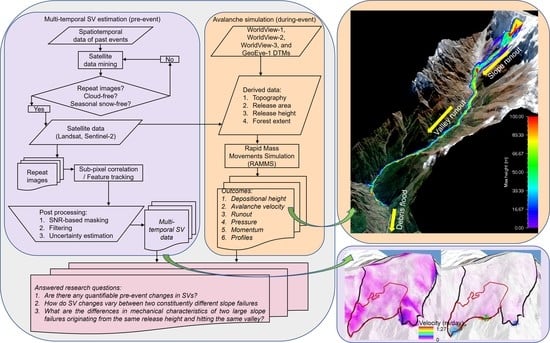
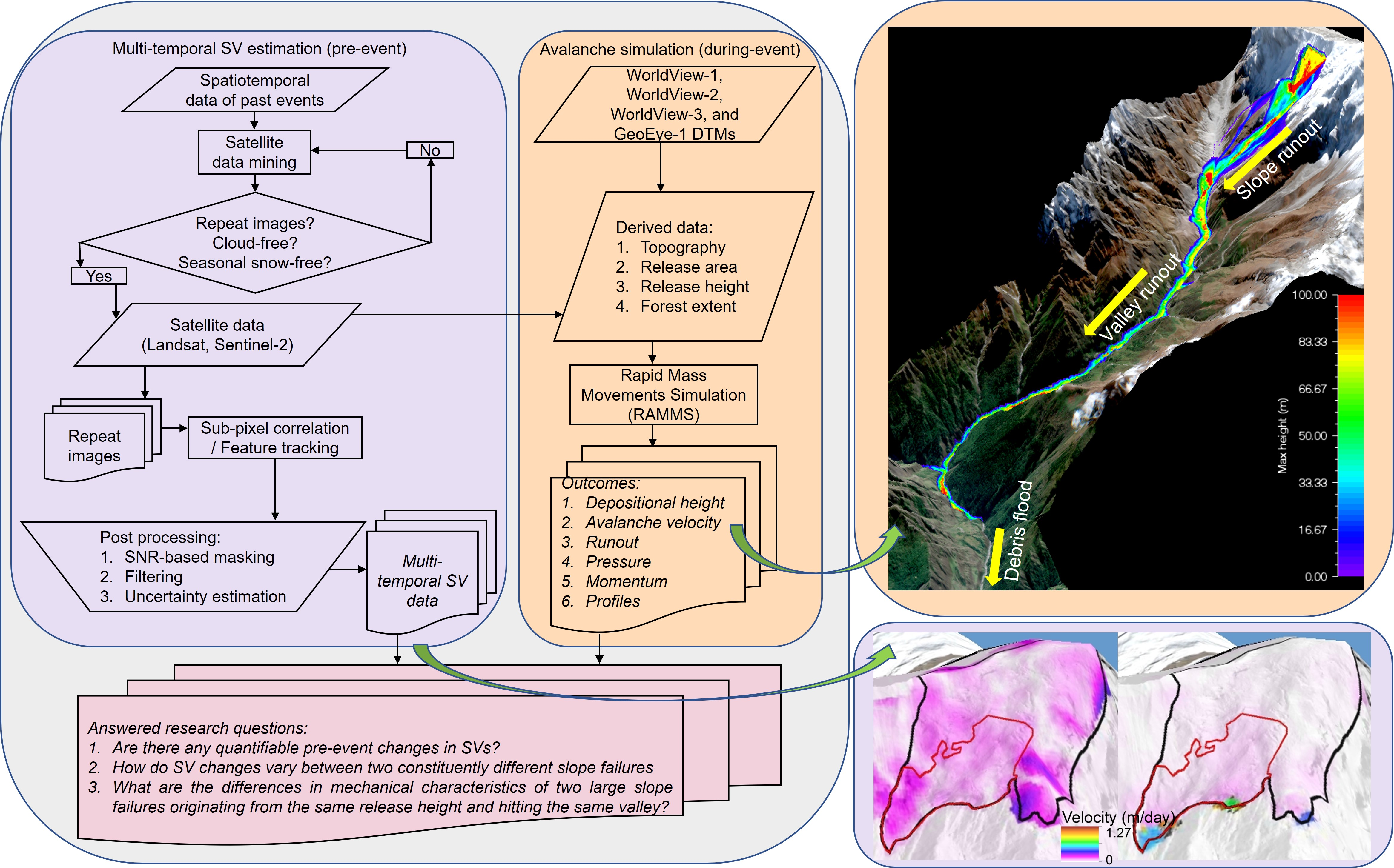
3. Materials and Methods

In addition to the high-resolution images obtained from Google Earth for visual analysis, we mainly used two remote sensing datasets for performing quantitative analyses: (1) multi-temporal satellite images for SV estimation and (2) high-resolution multi-temporal digital terrain models (DTMs) for Rapid Mass Movement Simulation (RAMMS) modelling. The details of these datasets are provided in

Table 1. Data used for SV estimations and RAMMS modelling.

Satellite Images
Acquisition Date	Scene ID/Band	Satellite/Sensor	Spatial Resolution (m/pixel)
1 September 2015	LC81450392015244LGN01/Panchromatic	Landsat 8/OLI	15
17 September 2015	LC81450392015260LGN01/Panchromatic	Landsat 8/OLI	15
3 September 2016	LC81450392016247LGN01/Panchromatic	Landsat 8/OLI	15
19 September 2016	LC81450392016263LGN01/Panchromatic	Landsat 8/OLI	15
9 October 2016	S2A_OPER_MSI_L1C_TL_SGS__20161009T053631_A006780_T44RLU/B2	Sentinel-2/MSI	10
14 October 2017	S2A_OPER_MSI_L1C_TL_SGS__20171014T104205_A012071_T44RLU/B2	Sentinel-2/MSI	10
24 October 2018	S2B_OPER_MSI_L1C_TL_MTI__20181024T090955_A008525_T44RLU/B2	Sentinel-2/MSI	10
24 October 2019	S2A_OPER_MSI_L1C_TL_EPAE_20191024T082325_A022653_T44RLU/B2	Sentinel-2/MSI	10
18 October 2020	S2A_OPER_MSI_L1C_TL_VGS1_20201018T072817_A027801_T44RLU/B2	Sentinel-2/MSI	10
27 December 2020	S2A_OPER_MSI_L1C_TL_EPAE_20201227T062601_A028802_T44RLU/B2	Sentinel-2/MSI	10
16 January 2021	S2A_OPER_MSI_L1C_TL_EPAE_20210116T063033_A029088_T44RLU/B2	Sentinel-2/MSI	10
26 January 2021	S2A_OPER_MSI_L2A_TL_EPAE_20210126T074559_A029231_T44RLU/B2	Sentinel-2/MSI	10
5 February 2021	S2A_OPER_MSI_L2A_TL_VGS1_20210205T082130_A029374_T44RLU/B2	Sentinel-2/MSI	10
DTM Details
Date Range for Stereopairs	Satellite	Source Link/Reference	Spatial Resolution (m/pixel)
1 September 2015–5 October 2015	WorldView-1 and WorldView-2	[21,36,37,38]	2
10–11 February 2021	WorldView-2, WorldView-3 and GeoEye-1	[21,37,39,40]	2

. The image IDs of the satellite images used for visual analysis are provided in the respective figure captions. The overall workflow, designed to investigate the pre-event and during-event flow characteristics, is depicted in Figure 2.

3.1. Surface Velocity (SV) Change Estimation

We used the Co-Registration of Optically Sensed Images and Correlation (COSI-Corr) tool [41], which works as a plug-in module to the Environment for Visualizing Images (ENVI) software for estimating horizontal displacement fields. COSI-Corr implements a phase correlation method based on the Fourier Shift Theorem and the retrieved relative displacement between an image pair is a resultant of an iterative, unbiased process, estimating the phase difference of their Fourier transform [41]. The standard outputs are in the form of East–West (EW) displacement, North–South (NS) displacement, and signal-to-noise ratio (SNR), and the absolute displacement is calculated as the square root of the sum of squares of the EW and NS displacement components. This displacement can be divided by various units of time, i.e., day in the present study, to obtain the SVs. The typical correlation accuracy achieved at sub-pixel resolution by COSI-Corr is as high as 1/20–1/10 of the spatial resolution of an image pixel [42].

The panchromatic band (Band 8) of Landsat 8 Operational Land Imager (OLI) and blue band (B2) of Sentinel-2 MultiSpectral Instrument (MSI) are the preferred bands for obtaining glacier and mass movement SVs [43,44]. Landsat 8 images were downloaded from the United States Geological Survey’s (USGS’s) EarthExplorer portal [45] and Sentinel-2 images were downloaded from the Copernicus Open Access Hub [46]. A 15 m/pixel resolution Landsat 8 Panchromatic band was selected for the SV estimation of SF1, as appropriate Sentinel-2 data was not available during September 2015. We found cloud-free Landsat 8 images covering 1–17 September 2015 and 3–19 of September 2016, with identical surface conditions for comparing the same duration SVs in the two consecutive years prior to SF1. We did not go back farther than one year before SF1 as it was primarily a frontal block failure and the critical ice load conditions for such events vary significantly from one year to another in this region [47]. The selected image pairs clearly highlighted the effect of this aspect on the estimated SVs. In fact, SF1 is a recurring frontal ice-block failure and we identified a previous similar event in early 2000 (Figure 3). In contrast, SF2 being primarily a landslide causing an ice-bedrock failure, we opted to perform yearly SV observations for it, starting from 2016 with good temporal availability of Sentinel-2 images. We again ensured cloud-free and similar surface conditions by selecting all the images from October, and this approach significantly reduced uncertainties. For SV observations ~40 days prior to SF2, we again opted for Band 2 of Sentinel-2. The presence of seasonal snow was unavoidable in this case. In order to effectively deal with mountain shadow, which was covering the entire SF2 hanging glacier uniformly during these ~40 days, we first clipped and then contrast-stretched the SF2 site in all the scenes by comparative histogram matching. Afterwards, we performed COSI-Corr processing only for this contrast-stretched part and the obtained results were considerably good with acceptable uncertainties (

Table 2. Estimated uncertainties in SVs. Please note that Cosi-Corr provides the displacement values, which are divided by the number of days between the image pairs to obtain velocities, explaining the corresponding, seemingly low, uncertainty values.

Correlated Pair (Represented by Acquisition Dates)	Cumulative Uncertainty (±cm/Day)
1–17 September 2015	2.13
3–19 September 2016	1.25
17 September 2015–19 September 2016	1.48
9 October 2016–14 October 2017	1.19
14 October 2017–24 October 2018	1.24
24 October 2018–24 October 2019	1.56
24 October 2019–18 October 2020	1.23
27 December 2020–16 January 2021	2.53
16–26 January 2021	3.21
26 January 2021–5 February 2021	31.70

).

Lacroix et al. [43] suggested to keep the window size for COSI-Corr processing as a compromise between the robustness of large windows and the ability of smaller windows to detect motions of rather small objects. Thus, we tried several window sizes and the most effective window size for our study site with the least uncertainties for both Landsat 8 and Sentinel-2 was found to be 32 × 32 window. We used this window for further processing all the data presented in this study. In the post-processing stage, we applied two of the filters effectively used by previous studies (e.g., [48]) to make the results more robust. Using the SNR filter, pixels with low SNR values (SNR < 0.90) were masked as poorly correlated pixels. Using the magnitude filter, we masked the abrupt values, assuming that the movement may not change abruptly but gradually [42], thus obtaining spatially smooth SV maps. However, we intentionally did not apply the magnitude filter for observing yearly movements as we wanted to identify the localised zones showing anomalous movements on a yearly scale. This approach perfectly served the purpose, as we could see the gradual spread of the stress field along the indentation for SF2 hanging glacier with each passing year until 2019.

3.2. Surface Velocity Uncertainty Estimation

The uncertainty introduced due to possible orthorectification errors may result in some minor sub-pixel-scale horizontal shifts in the Landsat 8 and Sentinel-2 images. However, in case of imageries for the same path and row used within this study, the orthorectification uncertainties affecting SV estimations are negligible [49]. Eventually, for estimating the cumulative uncertainties in our SV estimates, we adopted the approach suggested by previous studies (e.g., [48,50]). We sampled all the pixels representing the stable terrain devoid of ice and vegetation. For these stable pixels, the overall mean and standard deviation of displacements were summed up and divided by the temporal separation of the correlated images to obtain the overall uncertainty per correlated scene-pair. The estimated uncertainties are provided in Table 2 and were of the same order of magnitude as reported by the previous studies (e.g., [48,50]), except for the last pair of 26 January 2021–5 February 2021, owing to extreme snow cover in 5 February 2021 image.

3.3. Rapid Mass Movement Simulation (RAMMS)

The RAMMS tool for mass movement modelling, developed at the Swiss Institute for Snow and Avalanche Research, was successfully implemented for high mountain regions, such as the Alps (e.g., [51,52,53]), Andes (e.g., [54]), Himalaya (e.g., [55]), Southern Alps (e.g., [56]), Tatras (e.g., [57]), and others for realistic thermomechanical simulations. The RAMMS tool [13,25,58] has a user-friendly interface that allows for the integration of state-of-the-art numerical solution methods with input parameters derived from DTMs and satellite images or maps. An efficient second-order numerical solution of the depth-averaged avalanche dynamics equations forms the core of this programme [25]. More specifically, the model relies on the two-parameter Voellmy model, which is actually field calibrated using data from a real scale avalanche test site in Vallée de la Sionne, canton Valais, Switzerland [25]. The usual input parameters consist of topography, release area, release height, forest extent, and calibrated frictional coefficients, while the modelled output includes all types of mechanical parameters, such as avalanche velocity, momentum, flux, pressure, runout, and depositional height. Generating input data for this programme is straightforward as all the input parameters can easily be derived from the DTM and satellite images in the form of geographical information system (GIS) compatible shape files. The software manual provides sufficient details on how the tool works and how various frictional coefficients and input parameters can be manipulated to obtain the most realistic simulations. Detailed information on RAMMS and its input and output parameters can be downloaded from the software manual webpage [59]. More importantly, not long ago, a rock/ice avalanche model capable of modelling both extreme cases, i.e., avalanches containing mainly ice (e.g., SF1 in the present study) as well as avalanches that mainly consist of rock debris (e.g., SF2 in the present study), was embedded in the RAMMS software and was already successfully used by several case studies worldwide [60].

The hazard potential of many of the recent rock/ice avalanches, including SF2 in Chamoli, has been complex to comprehend, due to the extreme flow transitions among the constituents, i.e., ice, snow, and debris, and the temperature of the material. The proportion of the constituents (ice, snow, and debris) usually decides whether the dry fluidised (powder avalanches) flow regime would prevail, or a fluid-lubricated (debris flows) flow regime. The thermomechanical properties of the material entrained by the avalanche often determine its flow regime and modelling rock/ice avalanche speed and runout, and therefore requires a thermomechanical model accounting for the melting and lubricating properties of the entrained material, which is usually a mixture of snow, ice, water, and debris [13,58]. RAMMS is capable of modelling the thermomechanical regime of various types of avalanches, and therefore we used it as a tool to model during-event flow characteristics of SF1 and SF2.

High-resolution DTMs are extremely useful for geomorphology and mountain hazard research [61,62] and are most preferred for RAMMS simulations, as they inform the model about all the obstructions and natural dams to employ the most appropriate frictional parameters for a particular event. Fortunately, we have the availability of both pre-event and post-event high-resolution (2 m/pixel) DTMs covering SF1 and SF2 (Table 1). These DTMs were used in a study by Shugar et al. [21] and were derived by Bhushan and Shean [36] and Shean et al. [40] from the stereopairs of WorldView-1, WorldView-2, WorldView-3, and GeoEye-1 satellite images. Table 1 provides all the related references detailing the generation and characteristics of these DTMs. These DTMs allowed us to precisely demarcate and estimate the release area and volumes of SF1 and SF2 through DTM differencing as input to RAMMS. These areal and volumetric estimates are detailed in the Results and Discussion Sections. Another model input has to be the avalanche return period, which is pre-defined in the model as 10 years, 30 years, 100 years, and 300 years, representing various known or hypothetical recurrences. For SF1, we examined historical data and found it to be a recurring event, once the hanging glacier reaches its critical geometry. We could confirm that nearly 16 years ago, an event of same areal scale occurred at the SF1 site (Figure 3). Therefore, an average return period of 10 years was selected for SF1. This also translated in the simulation results in which the simulated SF1 avalanche followed the exact depositional boundaries that were observed in the after-event satellite images. We further ran the model using 30 years as the return period and the results were not equally comparable to the after-event satellite images that we derived using 10 years as the return period. On the other hand, SF2 predominantly consisted of rock debris [21] and was more suited for simulation within debris flow module of RAMMS, without a need to define the return period. Considering that both SF1 and SF2 were over 10 × 10⁶ m³, the avalanche volume category within RAMMS was set to “Large”. The model also takes into account the forest cover present along the avalanche path as an important input parameter, since vegetation provides resistance to the avalanche front. We digitised the forest mask using satellite images acquired prior to both the events. SF1 was mostly uninterrupted by any forest cover, while SF2, being a larger event, encountered dense vegetation along its path in lower reaches of the valley. Considering that SF1 was majorly an ice avalanche, for the avalanche core at rest, we used a density of 850 kg m⁻³ as recommended by Margreth et al. [53]. For SF2, considering the suggested rock:ice proportion [21] of 80:20 and the predominance of metamorphic rocks at the avalanche site [23], we inputted a density of ~2050 kg m⁻³ [63]. As the final vital input to RAMMS, the Coulomb friction (μ) and the turbulent friction (ε) are defined. The friction values μ and ε strongly depend on the return period and avalanche volume, and, in our study, owing to high-resolution DTMs and temporal image analysis, we were certain of these input parameters. The friction values, μ and ε, depend on the configurational energy content of the avalanche core [13], and in the avalanche module used for SF1 simulation in RAMMS, if a calculation is obtained with constant friction values, no terrain undulations and forest areas are considered. Therefore, for SF1, we opted for the variable friction values, which are automatically estimated by RAMMS, based on DTM-derived parameters (slope angle, altitude, and curvature), and we further provided forest information and the global parameters of the return period and avalanche volume. In case of SF2, the debris flow module of RAMMS needed to be initialised through a carefully selected combination of μ and ε, calibrated using the documented [21,22,23,24] time- and flow-related details of the event. This calibration was achieved through the observed runout extent on the post-disaster satellite imagery and the reported debris flow zones, flow heights, and velocities [21,22,23,24]. Thus, the model was precisely calibrated through extensive iterations to define the optimal friction values of μ and ε as 0.13 and 200 ms⁻², respectively. These values correspond well with the suggested range of values in the RAMMS manual.

A general topic of previous investigations for SF2 has been to explain the possible source of entrainment material, which led to such an enormous debris flow. A recent study [29], based on field observations, suggests that the vast deposits of the 2016 event might have been a possible source of material, which significantly enlarged the volume and extent of SF2. To investigate this aspect, we further used the erosion module in RAMMS while simulating SF2. We provided variable depths of sediment erosions between 2–8 m, based on the simulations by Jiang et al. [22], in the upper reaches of Ronti Gad, in order to model the increase in volume and velocity of SF2 as it travelled along the channel. This erosion corresponds to the material that aids the entrainment of the avalanche front. Supplementary Materials Files (Video S1: Simulated SF1 event, Video S2: Simulated SF2 event) of this paper provide a 3D visualisation of the RAMMS modelling results.

4. Results and Discussion

We present and discuss the main results of this research under the following subheadings, focussing on the pre-event and during-event flow characteristics of SF1, the long-term and short-term pre-event flow characteristics of SF2, and the simulated during-event runout characteristics of SF2.

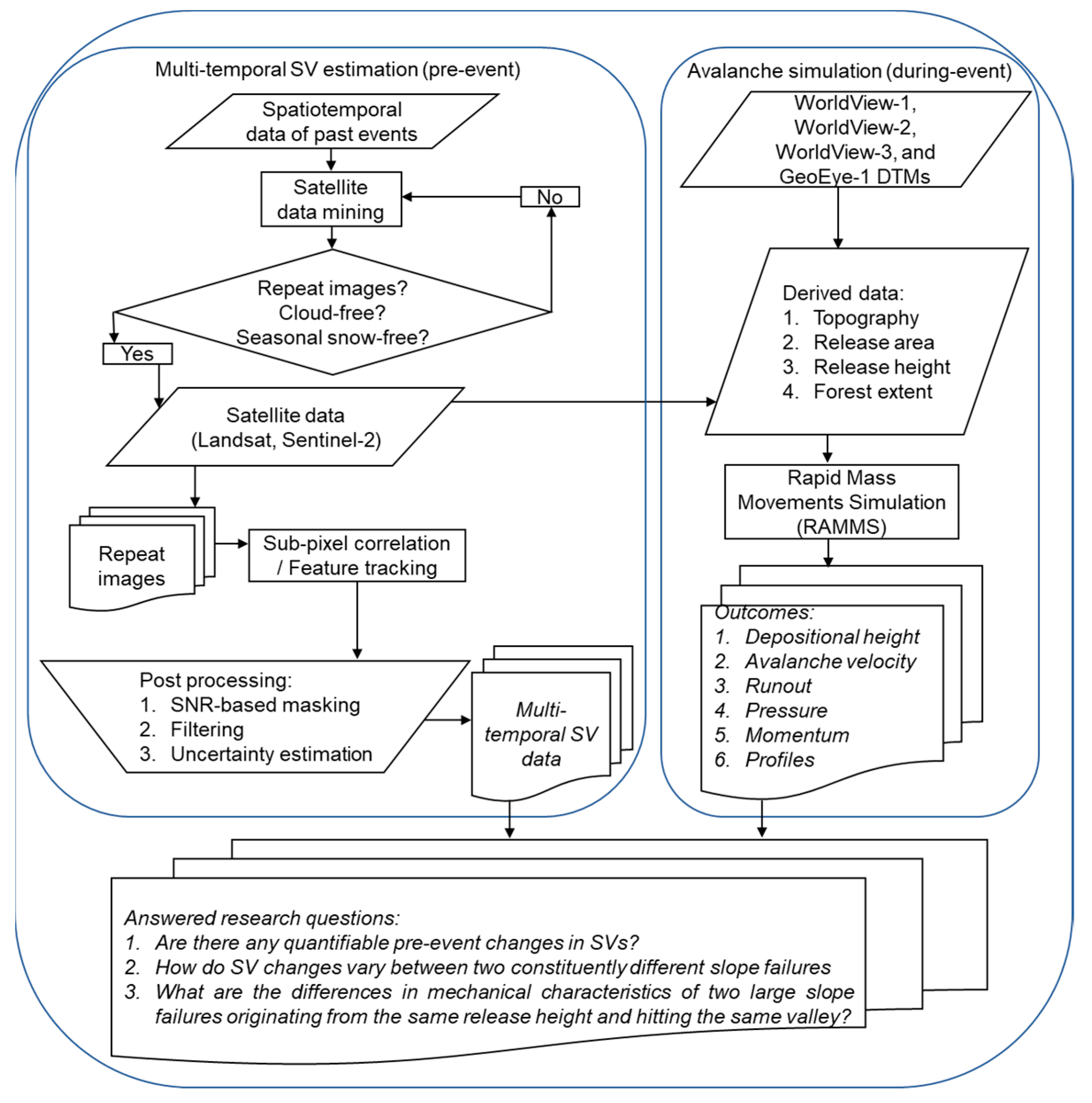
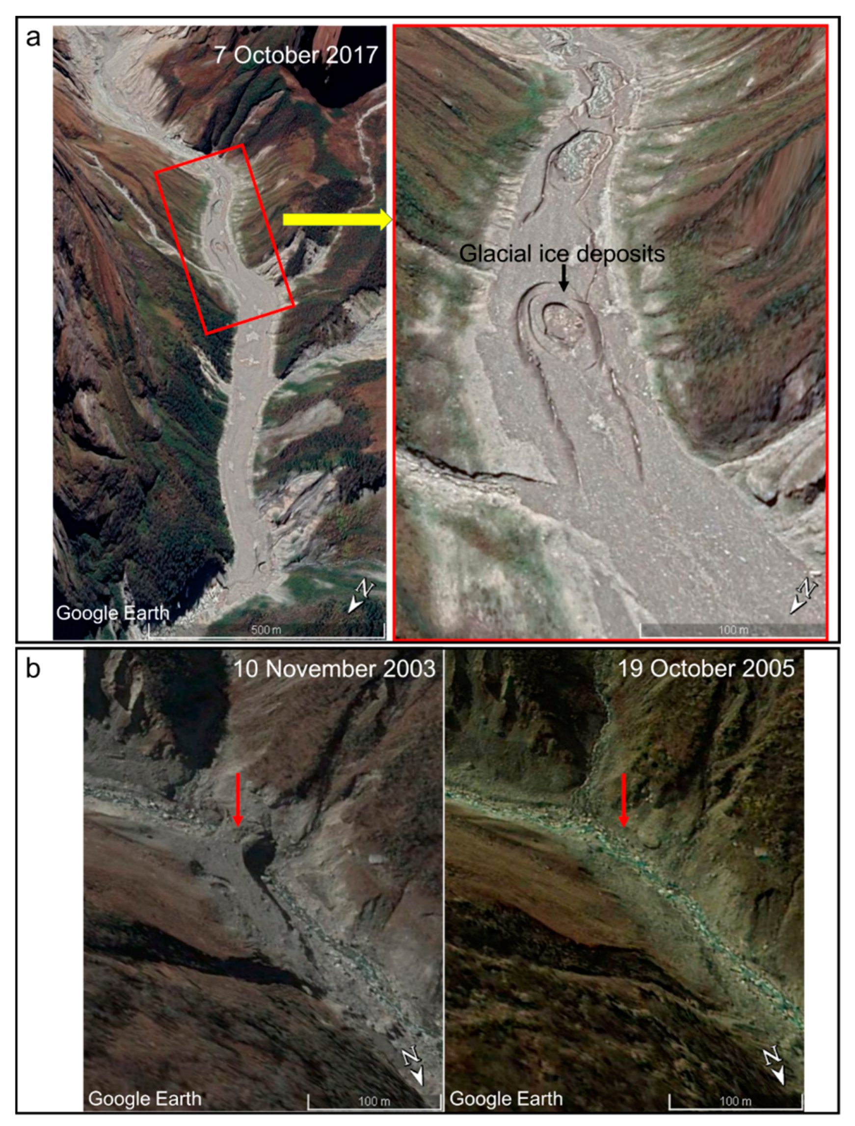
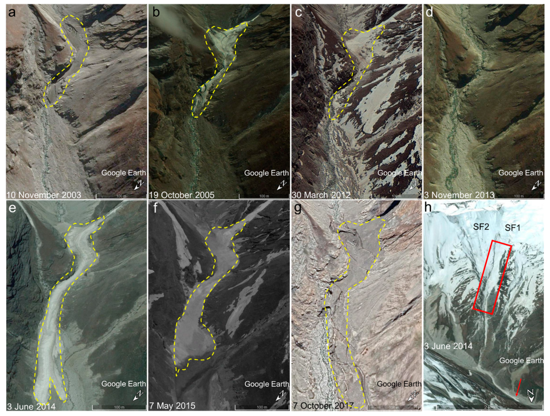
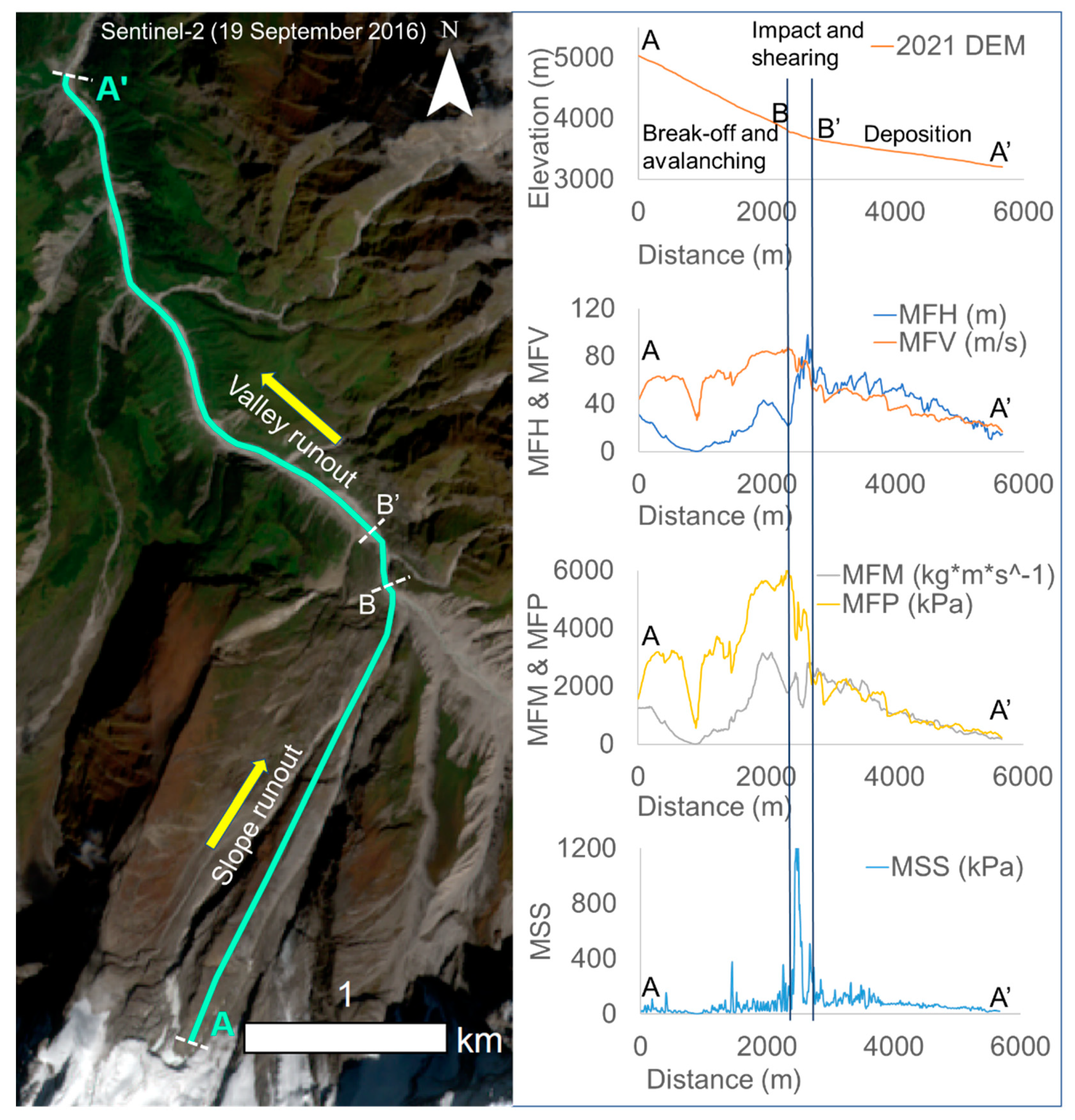
4.1. SF1: Key Observations and Pre-Event and During-Event Flow Characteristics

SF1 site (Figure 1 and Figure 3) appears to be a hotspot for ice avalanching from the same initiation zone. The maximum cross-sectional lengths and area of the broken part of the hanging glacier during SF1 were ~0.57 km (across the flow), ~0.92 km (along the flow), and ~0.28 km², respectively. SF1 was a frontal block failure and the multi-temporal DTMs of 2021 and 2015 provided by Shugar et al. [21] helped us to estimate a volume of ~10 × 10⁶ m³, corresponding predominantly to the glacier ice and possibly some seasonal snow. Using multi-temporal satellite images, we observed at least two major and comparable slope failure events at the SF1 site during the past two decades. These events were spaced ~16.5 years apart and they produced exactly the same indentation (Figure 3), marked by the dashed red curve in Figure 1c. For the earlier event, the 3D perspective views in Figure 3a depict the avalanched zone, and by using all the available Landsat images, we could narrow-down the timing of this event between January and April 2000. Similarly, the 3D perspective views in Figure 3b highlight the repetition of another avalanche (called SF1 in this paper) at the same indentation site. Using freely accessible Sentinel-2 and PlanetScope [64] images, we could narrow-down the timing of SF1 between 19 and 24 September 2016.

To understand the enormity of SF2, there is a need to consider these events from 2000 and 2016 at the SF1 site. These events were large-volume (~10 × 10⁶ m³) ice avalanche events leading to large deposits of ice and debris (orange rectangles in Figure 3) in the avalanche deposition zone in a narrow mountain stream named Ronti Gad. This deposition, following the 2000 and 2016 events, covered a ~3.5 km length of the stream (Figure 3 and Figure 4). The thick ice-debris deposits from these events tend to persist for multiple years after the event. For example, some of the possible remnants of the deposits from the 2000 event could be observed even in 2005, more than 5 years after the event (Figure 5b).

Another observation made on multiple years images (Figure 5) is the significantly seasonally active nature of the avalanche slope (Figure 5h). In addition to the ice avalanches, these slopes are always susceptible to snow avalanches during the winter months (Figure 5). A ~500 m-long stretch of the valley, directly beneath the avalanche slopes, is mostly covered by compacted snow, ice, and debris (Figure 5). These deposits also often hinder the full flow of the narrow stream, as is evident in Figure 4b, building up the temporary zones of increased hydraulic gradient and developing the dammed water pockets along the stream. We identified one such seasonally active avalanche slope below SF1 and SF2 sites (Figure 5 and Figure 6). While in the 3 November 2013 image of Figure 5 we observe a clear stream devoid of any avalanche deposit from the previous event of 2000 or from subsequent snow avalanches, in the 3 June 2014 and the 7 May 2015 images, we see thick fresh avalanche deposits covering the stream valley. Figure 5h highlights the seasonally active avalanche slope below the SF1 and SF2 sites, which accumulates significant snow mass during winter, often leading to slope failures relatively smaller than SF1 and SF2, but still large enough to form a deposition zone of ~500 m to 1 km in length. This large volume of snow, ice, and debris can accentuate any subsequent slope failure events, such as SF2, which occurred in the winter of 2021. We observed the available images of these slopes, days before SF2. Figure 6 highlights the significant snow accumulation on the seasonally active slope on 2 February 2021, while on 5 February 2021 Sentinel-2 image, it could be seen that a fresh cumulative snowfall of ~112 mm [22] significantly added to the snow cover. Figure 6 additionally shows the developed indentation from where the hanging glacier broke on 7 February 2021, causing SF2. Terrain profiles for SF1 and SF2 slopes (Figure 7), representing the terrain before either of the reported events occurred, estimate the maximum slope reaching as high as ~37°. The reported average slope for the entire SF2 mass [24] was even higher at ~40°. These slope values are entirely within the most avalanche-prone slope range reported from this region [18].

COSI-Corr [41] is an efficient tool to estimate surface deformations and mass movements through the correlations between temporal images, even in the absence of ground-control points (GCPs). COSI-Corr was conclusively established in estimating the motion in mass movements [43,65,66,67,68], glaciers [44], and sand dunes [69], with the relative accuracy of co-registration and correlation up to ~1/20th of a pixel [41]. Thus, there were two prime objectives for us to assess the flow characteristics of SF1. First, to use COSI-Corr for quantifying the SV changes leading to SF1, and, second, to perform the simulation and flow analyses of the broken ice volume during the SF1 event using RAMMS model. We used the cloudless and snow-free Landsat 8 satellite Panchromatic band (15 m/pixel) to estimate the SV during 1–17 September 2015 (a year before the 2016 event) and for a similar period during 3–19 September 2016 (Figure 8a,b), immediately before SF1 and at the end of the yearly ablation season. We also estimated the yearly SVs during 17 September 2015 to 19 September 2016, highlighting the higher SVs in the avalanched zone of the hanging glacier (Figure 8a,b). Compared to 1–17 September 2015, the maximum SV in the avalanched part of the hanging glacier is ~5 times higher during 3–19 September 2016 (Figure 8b) and the formed stress is strikingly evident in the region that leads to SF1 (middle and rightmost images of Figure 8a). The average velocity at the yearly scale (~12.3 ± 1.5 cm/day) for the avalanched part of the hanging glacier is also ~2 times higher than the average short-term velocities (~6.8 ± 1.7 cm/day) (Figure 8b). The maximum SVs show a distinctly increasing trend before the event, while the overall average SVs do not follow a pattern.

The visualisation of the surface deformations caused by the load effects, through an estimation of the surface displacements, has proven effective in observing the development and trajectory of mass movements [67,70]. As early as 1973, SVs were measured for the first time on an unstable cold-based hanging glacier in order to predict its collapse [71]. The observed velocities were shown to increase as a power-law function of time, up to infinity, at the theoretical time of failure [71]. This is also the characteristic signature of the stress build-up as a critical phenomenon in the case of various other naturally occurring ruptures, such as earthquakes [72], landslides [73], and rockfalls [74]. Velocity measurements performed on cold-based Weisshorn and Mönch hanging glaciers in Switzerland further confirmed this behaviour [75]. The validity of an SV monitoring approach was demonstrated in 2014 by the successful prediction of a hanging glacier “break-off” from the south face of the Grandes Jorasses (Monte Bianco, Italy), 10 days prior to the event [76]. However, owing to logistic issues, such efforts were understandably limited in their spatiotemporal domain, and all relied on field data collection for SV estimations. Our observations in the cases of SF1 and SF2, highlight that remote sensing-derived SVs have large spatial coverage and sufficient continuity and can represent a cost-effective and safer way to monitor hanging glaciers, and possibly even predict large and dangerous ice-rock avalanches in certain cases. However, any possible future predictability certainly requires more research in this direction to identify the types of slope failures which show statistically significant trends in SVs.

The RAMMS simulation further revealed the flow characteristic of this entire SF1 event (Figure 8 and Figure 9), which lasted for ~3 min as per the modelled results. Based on the mechanical characteristics, the event can be divided into three prominent phases (Figure 9): (1) break-off and avalanching in transect AB, (2) impact and shearing in transect BB’, and (3) deposition in transect B’A’. Overall, the maximum velocity, maximum flow height, and maximum pressure reached were ~90 m/s, ~100 m, and ~6000 kPa, respectively. The avalanching following the frontal break-off continued for ~2300 m before it struck the valley. The flow velocity, momentum, and pressure reached their peaks during this phase. Immediately after the impact, the maximum shear stress reached its peak (~1200 kPa), and this zone of ~200 m signifies the shearing and fragmentation of the ice core (Figure 9). Finally, a depositional analysis in RAMMS simulates the deposition zone within a ~3000 m length along the Ronti Gad stream (Figure 8c). The maximum deposition height is as much as ~48.10 m in the middle regions of the deposition zone (Figure 8c), highlighting the magnitude of the SF1 event. This also points towards the possibility that SF1 in 2016 and the previous event in 2000 might have preconditioned the valley significantly in terms of sedimentation availability and topographic smoothness, leading to the enormity of debris flow during SF2 in 2021. We further generated the deposition outline for SF1 and it remarkably matched the ice-debris extent observed in 9 October 2016 post-SF1 Sentinel-2 image. In the Himalayan context, the modelled flow characteristics and mechanical parameters are comparable to those reported for the Gyari glacier avalanche in the Shyok Basin of the Indus River, which killed 139 people [55]. The volume of the Gyari avalanche was 4.31 × 10⁶ m³, as opposed to ~10 × 10⁶ m³ of SF1, but the maximum height of the deposits reached as high as 40 m [55]. The difference between the simulated maximum pressure for Gyari (~2500 kPa) and SF1 (~6000 kPa) was also proportional to the mass difference between the two events [55].

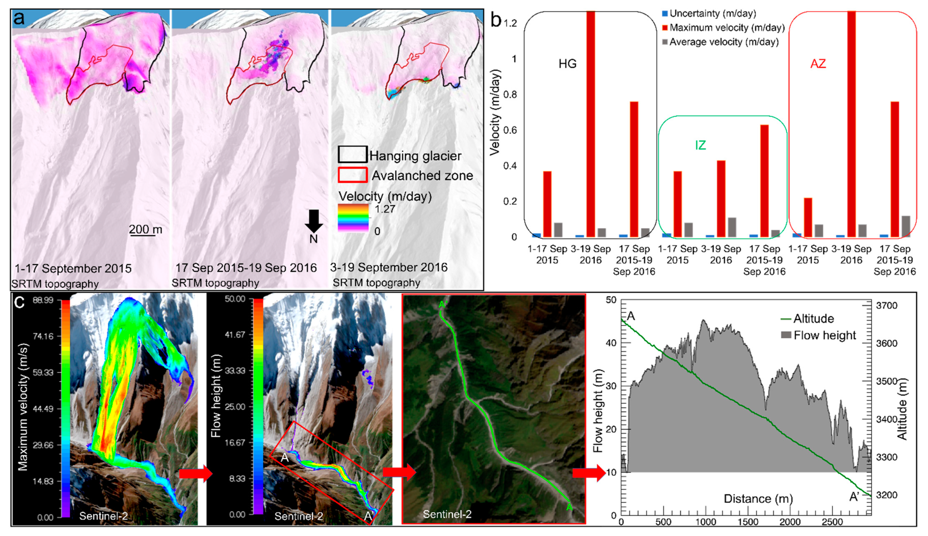
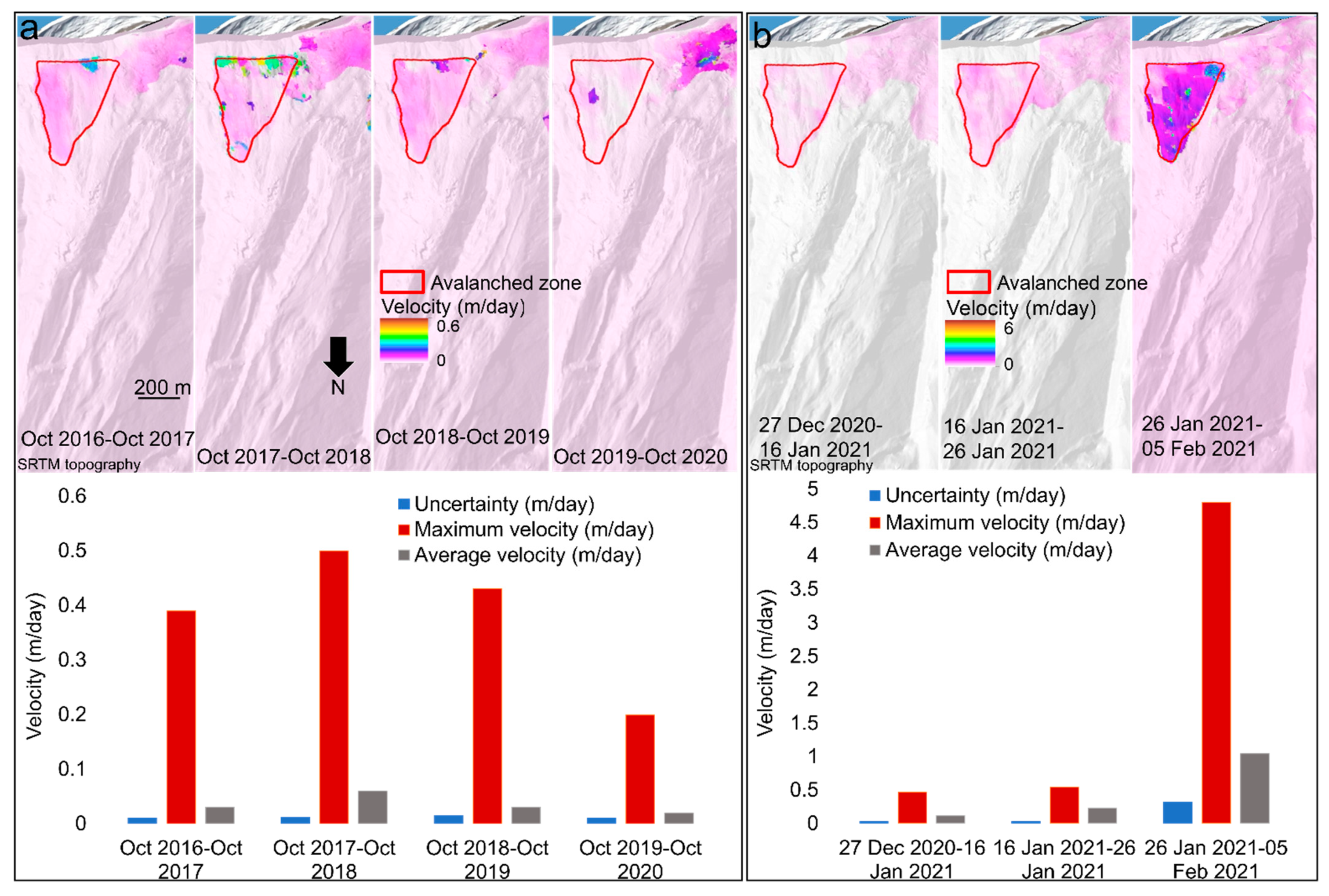
4.2. SF2: Long-Term and Short-Term Surface Velocity Evolution

We further monitored the temporal evolution in the SVs of SF2 hanging glacier. For the long-term yearly SV estimation, we used available best quality multi-temporal Sentinel-2 images from the October months of all the years, to ensure similar shadow and surface conditions. Cloud-free images from the September months were not available for some of the years. 10 m/pixel bands of Sentinel-2 images have been reported to be extremely useful in detecting precursory motions in the mass movements using COSI-Corr [43]. We generated a time-series of the yearly SVs (Figure 10a) to observe the long-term changes and the zones of the hanging glacier showing anomalous SVs. During October 2016–October 2017, we can observe anomalous ice movement fields developing in SF2 break-off zone of the hanging glacier, below its bergschrund (a large crevasse often marking the head of a mountain glacier), with the maximum SV reaching as high as ~39.2 ± 1.2 cm/day, while the average SV for the entire hanging glacier is ~2.9 ± 1.2 cm/day (Figure 10a). The average SV kept on fluctuating through 2017–2019; ~5.9 ± 1.2 cm/day during 2017–2018 and ~3.1 ± 1.6 cm/day during 2018–2019 (Figure 10a). However, the most interesting observation is the distinct stress field growing across the entire break-off zone, below the bergschrund of the hanging glacier, with the maximum SVs reaching up to ~51.3 ± 1.2 cm/day during 2017–2018 (Figure 10a).

These estimations are in accordance with the conclusions provided by Shugar et al. [21], where they report the destabilisation in SF2 mass starting from 2016, i.e., after SF1, and displaying maximum displacements during the summer months of 2017 and 2018. These SV values indicate that SF2 mass was already unstable post-SF1, and experienced significant displacement by 2020. The indentation that was almost invisible in 2016, grew to be as large as ~60–80 m by October 2020 (Figure 11), highlighting the major displacements during this period. The heavy precipitation [26,29] in the early weeks of February 2021 further added to this large, destabilised volume (~27 × 10⁶ m³) of rock, ice, and snow, leading to SF2. In fact, as per the Supplementary Data provided by Jiang et al. [22], the cumulative snowfall only on 5 February 2021 was ~112 mm, considerably higher than any of the days of that winter season.

SF1 in itself was a fairly large event that exerted a huge pressure of ~6000 kPa at its impact point, and the localised tremor could have initiated the destabilisation in the bedrock of SF2 hanging glacier below its bergschrund. A valid question here might be that why a similar intensity 2000 event at SF1 site did not trigger the destabilisation in the bedrock of SF2 hanging glacier. The possible answer lies in the timing of both these events at SF1 site. The 2000 event occurred in the winter months, while the 2016 SF1 occurred in September, i.e., at the end of summer, when the bedrock is more prone to detachment. The powerful impact of SF1 might have been sufficient to cause such detachment in the bedrock of SF2 hanging glacier, which continues to grow during the following years (Figure 11). However, it will need a separate detailed investigation to conclusively prove if impacts such as SF1 can trigger further glacier detachments. Here, we also report the short-term SV changes during the ~40 days prior to SF2 (Figure 10b). While the average SV during 27 December 2020–16 January 2021 was ~11.9 ± 2.5 cm/day, it nearly doubles to ~23.2 ± 3.2 cm/day during 16–26 January 2021, and reaches over eight times this figure to ~105.2 ± 31.7 cm/day during 26 January–5 February 2021 (Figure 10b). However, an even more dramatic increase is recorded in the maximum SVs, showing a ~10-fold rise during these ~40 days, with the maximum SVs reaching ~481.8 ± 31.7 cm/day by 5 February 2021, 2 days prior to SF2 (Figure 10b). However, these estimates should be interpreted with care due to the proportionally high uncertainties associated with the SV measurements for the 26 January–5 February 2021 period (Figure 10b), owing to significantly high snow cover and poor illumination conditions in 5 February 2021 Sentinel-2 image (Figure 6b, Figure 11f). Such conditions are reported to significantly affect the quality and accuracy of SV estimations [44], and therefore, we cannot conclusively say if the derived SVs for the 26 January–5 February 2021 period refer to actual displacements or are majorly a result of image artifact. Nevertheless, these short-term SVs provide a sequential picture of the pre-event flow characteristics, during a period of approximately one month, leading to SF2.

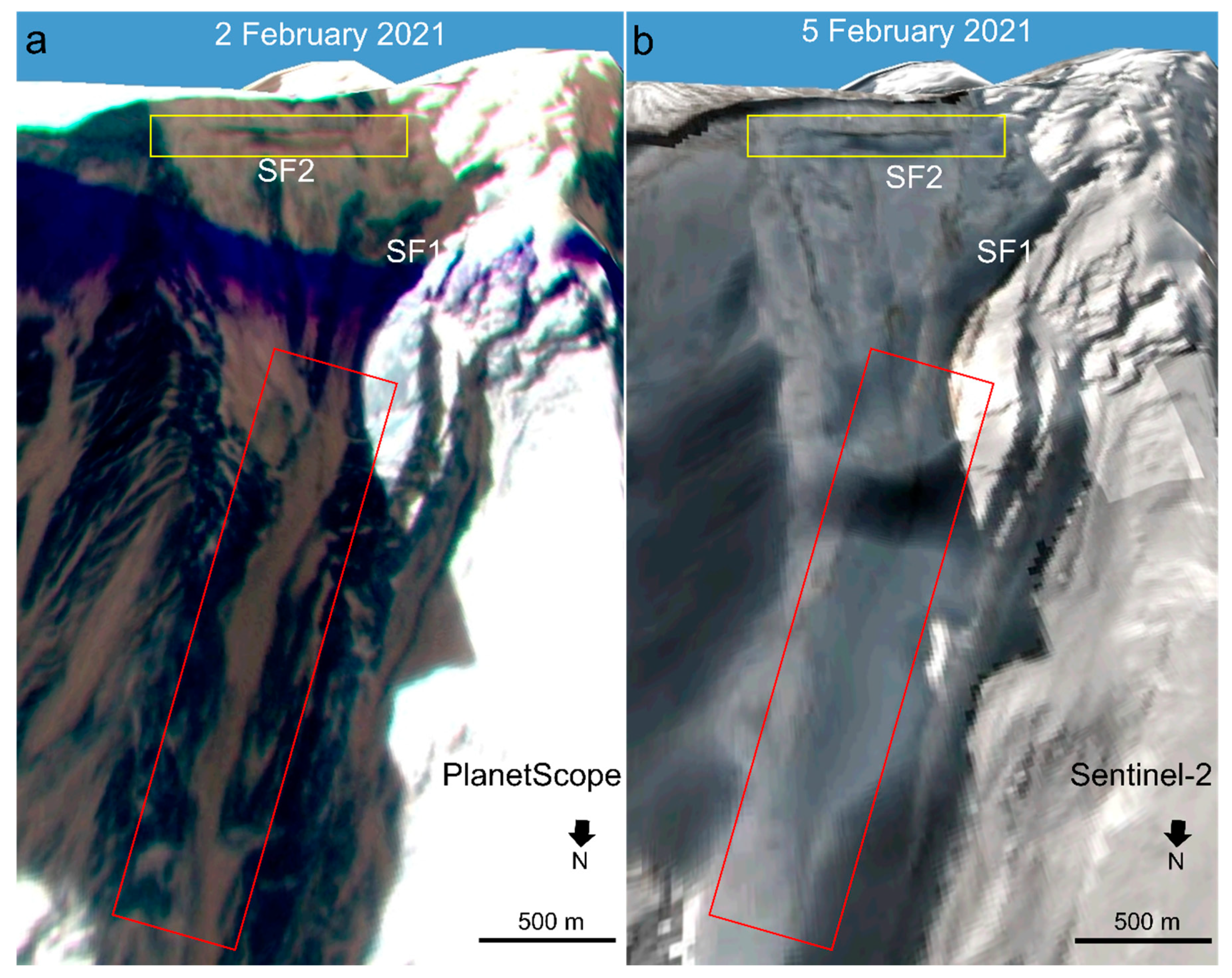
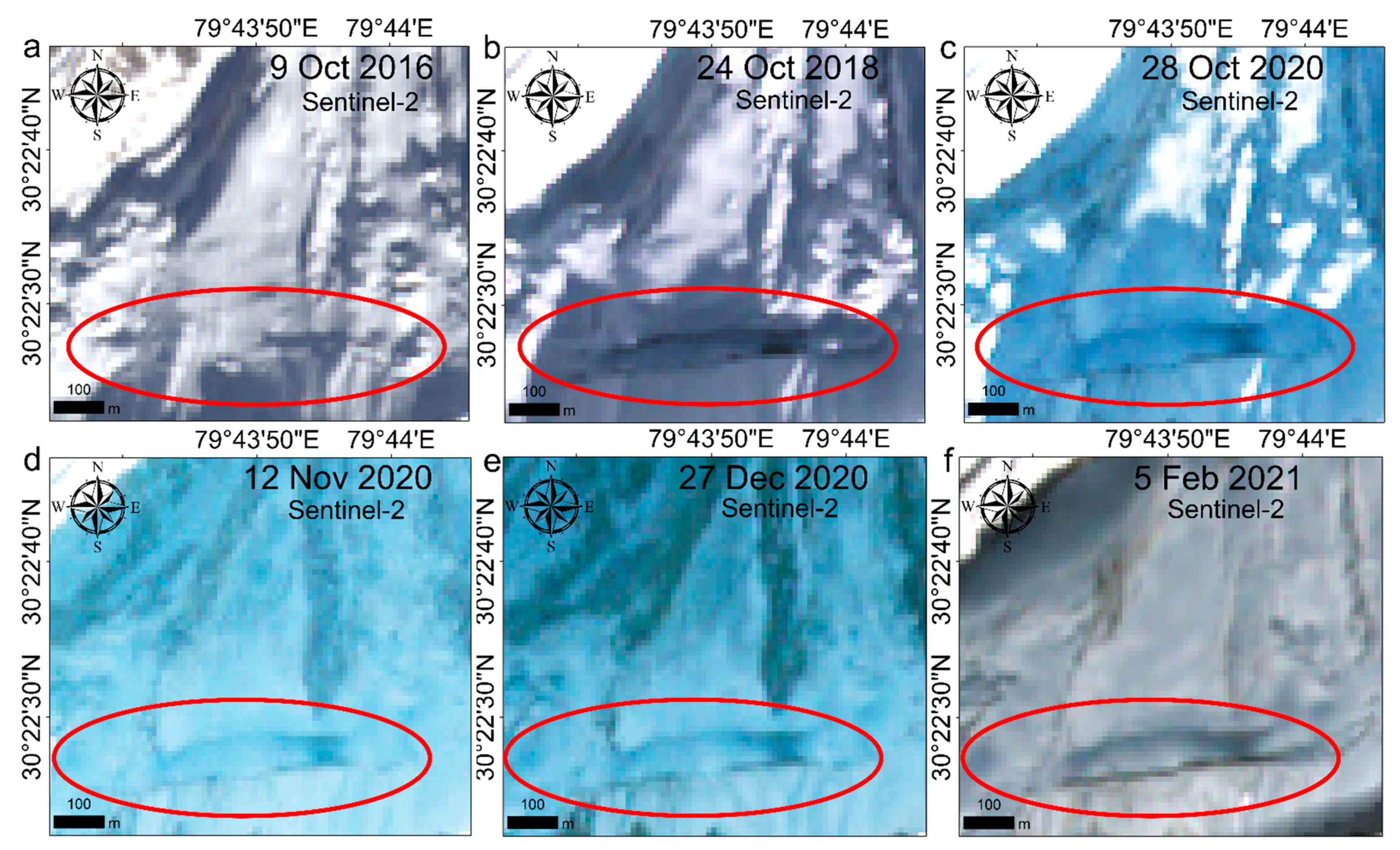
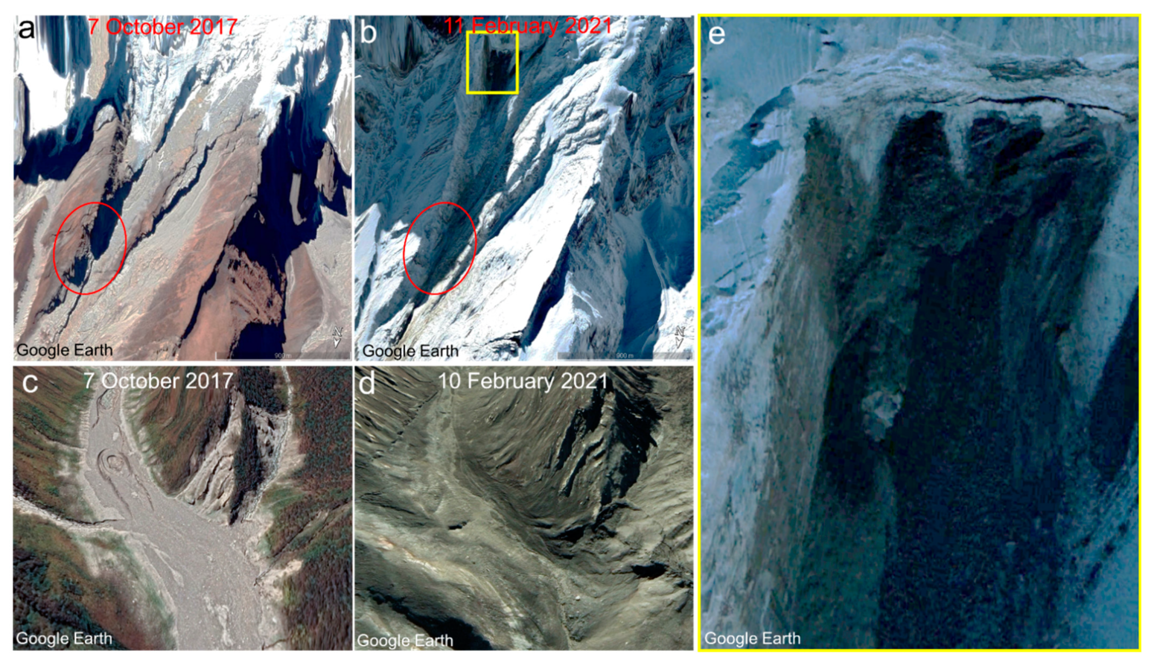
4.3. SF2: Key Observations and During-Event Flow Characteristics

The total area of the avalanched part of SF2 hanging glacier was ~0.27 km² with the maximum length of ~850 m. The destabilisation in the bedrock started after SF1 in 2016 at an elevation of ~5600 m asl (Figure 11), and on 7 February 2021, this sliding mass of rock and ice crashed into the Ronti Gad valley at an elevation of ~3800 m asl. We simulated this SF2 event using high-resolution DTMs and RAMMS model. We contrast-stretched a high-resolution image of 11 February 2021 (Figure 12e), and the scar certainly suggested a significant removal of bedrock, as also modelled by Shugar et al. [21]. This event started as a landslide and turned into a rock-ice avalanche. Real-time images provided by PlanetScope [64] suggest that before Raini village, SF2 turned into a more fluidised debris flow, causing a flash flood in Rishiganga River. This flash flood took nearly 27 min to cover the ~6 km of the distance between Raini village and Tapovan town (Figure 13), clocking a disastrous velocity of ~4 m/s. This velocity is comparable to those of several reported flash floods in mountain catchments and is capable of carrying a significant amount of debris and sediment to a large distance, destroying any obstructions in the path [77,78]. The large debris and sedimentation spread along the river channel after SF2 is visible on the 10 February 2021 Sentinel-2 image of Figure 14d.

The RAMMS simulation provided us an informative account of the mechanical characteristics of SF2 (Figure 15), which further helped us in deciphering the various zones of this entire event (Figure 16). The reported accounts [21,22,23,24,29] based on field validation, air surveys, and the visual interpretation of satellite images suggest that the total distance between SF2 site and the end of the rock-ice avalanche deposition zone was ~13 km (~2 km of mountain slope and ~11 km of river valley). From this point, the deposits started becoming more fluidised and turned into a debris flood [21]. The same published sources [21,22,23,24,29], using seismic modelling and videographic evidence provided by the local population, also put a constraint on the timeline of this event. The initial slope failure occurred at 10:21 Indian Standard Time (IST) (4:51 Greenwich Mean Time (GMT)) and it took slightly less than a minute to hit the valley [21]. PlanetScope image taken at 5:01:51 GMT (Figure 13), shows the SF2 front at the exact bend before Raini village where the rock-ice avalanche started turning into a debris flow. This indicates that SF2 rock-ice avalanche front took 10 min to travel to the transition point. However, this transition bend was also one of the sharpest and narrowest along the valley, stopping the runout and depositing the majority of the avalanched and entrained mass. This further consolidation of rock debris and ice along Rishiganga valley could have taken a few more minutes, as a long trail of avalanche can still be seen in Figure 13a. Thus, we calibrated our RAMMS model for the aforementioned distance and time to reach the optimal friction values of μ and ε. The final model outcome presented us with a time of ~13.5 min for the entire SF2 avalanche event, from slope failure until complete deposition. This is in accordance with the estimated timeline above and the simulated timeline provided by Jiang et al. [22]. This consistency in the spatiotemporal premise for the final outcomes gave us the needed confidence in the simulated mechanical parameters for SF2 (Figure 15 and Figure 16). The improving satellite remote sensing capabilities, such as the temporal resolutions, help to study natural hazards more efficiently, as in this case too, PlanetScope was able to capture the first image within ~10 min of the event, giving us a reliable timestamp for calibrating the model.

The maximum velocity reached by SF2 was ~65 m/s, while most of the flow height remains below 120 m (Figure 16). These values also correspond well with other studies; Shugar et al. [21] reported flow height of up to 120 m and the maximum velocity of 60 m/s for this event, while Jiang et al. [22] modelled the maximum flow height of 100 with the maximum velocity of 65 m/s. The maximum pressure reaches ~6000 kPa, while the momentum reaches ~4000 kgms⁻¹ in the GG’ transect (Figure 16). Based on the modelled mechanical characteristics, SF2 as a rock-ice avalanche can be divided into five prominent phases before it turns into a more fluidised debris flow in Dhauliganga River (Figure 16): (1) slope failure and sliding as slope runout (initial ~1800 m of transect GG’, i.e., GA); (2) impact and shearing (~1800–~2400 m of transect GG’, i.e., AB); (3) entrainment from valley sediments (~2400–~5000 m of transect GG’, i.e., BC); (4) liquefaction and rock-ice avalanche front propagation as valley runout (~5000–~8900 m of transect GG’, i.e., CD); and (5) deposition, detrainment, and transition into a more fluidised debris flood (~8900–~12,500 m of transect GG’, i.e., DG’).

In the first phase of the landslide, the detached mass travelled ~1800 m before it struck the valley. Our model results highlight an interesting and previously unreported aspect of this phase. At nearly 750 m below the terminus of the SF2 hanging glacier, we observed a dip in all the mechanical parameters, and, remarkably, we could also observe a dip in the difference DTM, highlighting the removal of significant rock volume by the SF2 rock-ice mass before it struck the valley (Figure 16). SF2 majorly consisted of rock volume and started as a landslide, and, therefore, when the large rock body hit the spur, it eroded it. The red ellipse in Figure 12 highlights this spur in the path of SF2 and the middle panel of Figure 16 shows the difference DTM highlighting the obliterated spur during SF2 propagation. This spur had a height range of ~4–74 m with an average height of ~25 m; The total area covered by it was ~31,078 m² and the total volume of this spur removed by SF2 was ~795,810 m³. This observation signified two aspects of this phase: (1) the model worked significantly well in predicting a hindrance in the flow, leading to the possible removal of this spur owing to the mechanical characteristics (high momentum and power) of the landslide, and (2) a significant rock volume of ~0.8 × 10⁶ m³ was further added to the avalanched volume of ~27 × 10⁶ m³ even before it reached the valley. Shugar et al. [21] postulated that the reason behind the intact lowermost part of the neighbouring larger eastern glacier post-SF2, might be the possibility that the avalanche became airborne for a while. A 3D visualization of our modelling result (Supplementary Materials Video S2) confirms that while the avalanche was airborne briefly, it soon became grounded and that could explain the obliteration of this spur. We perceive that the presence of this spur offered a topographic barrier to the lowermost part of the eastern glacier, causing a slight pause in SF2 propagation (hence the dip in the mechanical parameters), containing it within a channel, and becoming obliterated in turn. This topographic barrier and friction also caused some deformation and possible breakage of the SF2 mass, as is evident from the spikes in the shear stress profile in Figure 16.

In the impact and shearing phase, the SF2 mass hit the valley floor and all the mechanical parameters reached closer to their peak values during this phase. Immediately after the impact, the maximum shear stress reaches its peak (~1200 kPa) and this zone of ~600 m signifies the shearing and fragmentation of the rock and ice core (Figure 16). While the ice-debris from SF1 in 2016 mostly remains within ~3 km of the deposition zone, covering the main channel and surroundings, the SF2 event, starting from slightly steeper slopes, releases over ~2.5 times more of the rock-ice volume on the valley floor with previously deposited avalanche debris, significant seasonal snow (Figure 6b), and possibly dammed water ponds (Figure 4 and Figure 5). This impact could have led to considerable ice and snow melt through the substantial change in momentum (Figure 16), leading to the transmission of energy by the falling and sliding rock and ice along the stretch. This immense rate of change in momentum and power, once the avalanche hit the valley, also caused the large burst whose bang could reportedly be heard from as far as ~15 km from the avalanche site, and was later identified in the seismic readings from a station located over 100 km away [21]. For a similar event at Kolka in the North Ossetia–Alania region of the Caucasus Mountains in 2002, where a sliding hanging glacier of ~20 × 10⁶ m³ failure volume hit and eroded a small glacier, a broad estimate, considering that the substantial amount of energy was dissipated during the fall and impact, suggested that ~0.44 × 10⁶ m³ of ice could be instantly melted by a falling volume of 8 × 10⁶ m³ [79]. Considering that SF2 had a total volume of over ~27 × 10⁶ m³ and it travelled an almost similar drop height as Kolka, it could have melted at least 3 times of ~0.44 × 10⁶ m³ of ice instantly, i.e., ~1.32 × 10⁶ m³ of ice, corresponding to the ~1/4th of the total SF2 ice volume, due to the direct impact and frictional sliding. This can explain why in contrast to most previously documented rock avalanches, very little debris was found at the base of the failed slope [21]. The Kolka event too, similar to SF2, did not allow the fallen ice and debris to deposit in the vicinity of the fall, but led to an unprecedented runout distance of ~20 km, followed by flash mudflows. In such voluminous avalanches, granular friction can effectively be reduced by ice melt and associated fluidisation effects, leading to much larger travel distances than usual [79].

The next phase of SF2 consisted of entrainment from the valley sediments, mostly within the ~2400–~5000 m of transect GG’, i.e., in the BC region (Figure 16). Point C in Figure 16 marks the sharp turn in the channel where previous ice avalanches of 2000 and 2016 from SF1 site had stopped. While the majority of the ice-debris deposit from SF1 appears to have melted away before the SF2 event, we cannot ignore the enormity of SF1 deposits (Figure 4, Figure 5 and Figure 8), when the maximum deposition height reached as high as ~48 m. The SF1 event had not just altered the valley profile, but had also enriched it with significant volume of sediments and percolated meltwater in subsequent years. A mystery in explaining the long runout of SF2 has been that how only 20% of ice volume could displace nearly the entire 80% of rock volume, so far down the valley [29]. We propose that the long runout of SF2 was facilitated by the considerable entrainment from the valley sediments of past ice and snow avalanches (Figure 4 and Figure 5) during this phase of SF2 in the BC transect (Figure 16). To evaluate this hypothesis, we modelled two scenarios: (1) with the inclusion of differential erosion areas and erosion depth based on the modelled results of Jian et al. [22], and (2) without specifying the erosion areas and depth. By default, the model includes a critical shear stress that permits erosion only when the shear stress in any given cell exceeds the critical shear stress value for the onset of erosion. However, with the available information, i.e., in this case, the extent of SF1 deposits and modelled erosion by Jiang et al. [22], the inclusion of defined erosion zones can improve the model accuracy. RAMMS also provides the option to input erosion area parameters, and these were appropriately adjusted as per the instructions in RAMMS manual. Scenario 2 of not specifying the erosion areas and depth also meant that we had to consider a smaller turbulent friction (ε) parameter. While, for Scenario 1, after the model calibration, we opted for a value of ε = 200 m/s², representing a transition from a solid-dominated granular flow to a muddier flow owing to sediment entrainment, for Scenario 2, we chose a value of ε = 100 m/s², representing a relatively drier solid-dominated flow. As we expected, compared to Scenario 1, the rock-ice avalanche in Scenario 2 took nearly twice the time with an unrealistically low avalanche front momentum (only the ~1/3rd of Scenario 1), for reaching point G’ in Figure 16. This supports our assumption that the role of past avalanche deposits in entraining SF2 was considerably significant.

The subsequent phase of SF2 between ~5000 m and ~8900 m of transect GG’ (i.e., CD) does not only show a relatively constricted valley profile, but is also marked by dense vegetation along the channel, which offered considerable resistance to SF2 propagation. The rapidly changing shear stress, flow pressure, and maximum flow height values in Figure 16 highlight this aspect. This friction led to further liquefaction of the avalanche core and the front took the shape of a well-defined rock-ice avalanche between this ~5000–~8900 m of transect GG’, i.e., in section CD. Point D represents another sharp turn in the valley and allowed for the temporary accumulation of material, leading to rise in the flow heights (Figure 16).

The last phase of SF2 is marked by the deposition of transported material between ~8900 and ~12,500 m of transect GG’, i.e., section DG’. Transect HH’ in Figure 16 represents the place where Ronti Gad meets Rishiganga River and, from this point onwards, a vast volume of sediments and rocks were deposited, temporarily damming the river and forming a ~700 m long lake [21]. A deposition analysis in RAMMS resulted in the total deposition volume of ~15 × 10⁶ m³. The maximum flow height reached up to ~120 m. While Shugar et al. [21] also reported the maximum deposition height in the same range, based on DTM differencing, they reported the total deposition volume of ~8 × 10⁶ m³, between the Ronti Gad–Rishiganga River confluence and point G’ in Figure 16. There are two reasons why our deposition volume is larger: (1) we observed and quantified the deposition on a larger stretch of transect GG’, i.e., DG’, and (2) our deposition estimates are in real-time, representing the terrain just after the rock-ice avalanche stopped at point G’. Figure 17 clarifies this point further. The 2021 post-SF2 DTM was generated using stereopairs acquired on 10 and 11 February and, by then, a significant volume of deposits fluidised and escaped as the debris flood. After 24 h of the event, the sediment plume could be seen on satellite images ~150 km downstream of the source, and ~80 times of the normal turbidity could be observed ~500 km downstream within 8 days of the event [21]. This means that the deposited avalanche material continuously kept on fluidising, contributing to a constant, albeit gradually diminishing, debris flow. To evaluate our modelled deposition results, we hypothesised that while DTM difference elevations would show lower deposition heights, considering that they were generated using 10/11 February stereopairs, the profile pattern should match our modelled deposition heights. When we performed the profile analysis along four transects in the deposition region (Figure 16), we found that there was a remarkable similarity between the profile patterns between the modelled curve representing the deposition height immediately after the SF2 event on 7 February and the DTM difference curve representing the terrain on 11 February (Figure 17). This further proved the authenticity of our simulated results.

The SF2 event could be a result of the combined contribution of both the gradually destabilising slope and a deformational stress building up due to the winter snow accumulation load. A recent paper [47] suggested a possible polythermal regime for glaciers north of the study area, promoting both sliding and deformational forms of motion. Both pressure melting and creep-rate enhancement driven by stress concentration act as prime factors in producing noticeable surface motion under polythermal regime [80]. An approximate range for the existence of cold, polythermal, and temperate ice based on the relation between the mean annual air temperature (MAAT) and critical slope for failure on ramp-type glaciers [81] suggests that, for the average slope of SF2 site and assuming the polythermal nature of ice, a slope failure is possible within an MAAT range of −2.5 °C to −5 °C. The MAAT for SF1 and SF2 corresponds to ~−5 °C, based on the published data for Chamoli district [82], extrapolated to the SF2 site using a constant environmental lapse rate of −6.5 °C [83]. This means that such slope failures can become increasingly possible, irrespective of the seasons, with changing climatic conditions. In their review on avalanching glacier instabilities, Faillettaz et al. [84] identified three different types of instabilities depending on the thermal properties of the ice/bedrock interface. If cold, the glacier experiences a critical acceleration following the power-law up to the break-off, and a prediction of the final break-off is possible. The type of motion observed in case of SF1 is closer to a possible cold regime, indicating a possibility of predicting its future break-offs. In case of a temperate regime, water plays a key role in the development of instability, and critical conditions promoting the final instability can still be identified [84]. However, in the case of a partly temperate or polythermal regime, predicting the actual break-off becomes difficult. While SF1 and SF2 are different in their mechanical characteristics, in both these cases, we observe certain abrupt but characteristically different changes in SVs, which raises another research question concerning whether their thermal regimes are different despite being in proximity, or if they experience a transition/evolution in their thermal regimes. The temporal evolution observed in the case of SF2 might represent the instability in a glacier experiencing a rapid transition from a cold to a temperate glacier bed due to percolation through the detached headwall. This possibility makes our SV estimates relevant to possibly open-up a new research frontier on understanding the transition in thermal regimes of hanging glaciers in these mountains, and how this transition might make them more prone to slope failures.

5. Conclusions

This research started with targeting three key research questions (Figure 2) mentioned in the Introduction Section, and we successfully derived several useful conclusions for them. The change in satellite-derived SVs should further be explored as an important precursor of ice-rock avalanching, and its temporal observation in high mountains can prove to be extremely helpful for predicting several SF1-type future slope failure events. Our SV estimates prove that continuously improving temporal and spatial resolution of satellite datasets can be effectively employed in performing such observations at unprecedented spatiotemporal scales. We also observed how SV changes vary between two constituently different slope failures, i.e., SF1 and SF2. In the case of the landslide causing ice-bedrock failure, i.e., SF2, SV anomalies developed and disappeared gradually and could be observed even at yearly scales. However, that makes predicting the actual time of failure difficult. The observed increase in SVs days-to-weeks prior to SF2 should be interpreted with caution, as relatively higher uncertainties are associated with them, due to high snow cover and poor illumination in satellite images. More of similar case studies are needed to infer if other SF2-type events also experience an immediate surge in SVs prior to their occurrence. On the other hand, for the frontal block failure, i.e., SF1, the SV anomalies are more localised and pronounced closer to the time of slope failure, as the glacier attains its critical geometry (Figure 18). We further performed calibrated RAMMS simulations to infer the differences in the mechanical characteristics of the two large slope failures, i.e., SF1 and SF2, originating from the same release height and hitting the same valley floor. The simulated mechanical parameters were able to describe the during-event flow characteristics of both the events, and the changes in these parameters further helped in identifying the various zones of these mass movements.

Although the past events at SF1 site had not inflicted any direct damage to life and property, it is difficult to predict their future impacts in combination with other glacial hazards, such as SF2. While SF2 is an ice-bedrock failure, SF1 shows the characteristics of a frontal block failure as it tends to periodically replicate itself. More importantly, we can observe new ice accumulation at the avalanched slope of SF1 site since its last failure in 2016 (Figure 18). The hanging glacier is recovering its previous critical geometry before SF1, and ~0.052 km² (~20% of the total lost area in SF1) was recovered by October 2020 (Figure 18). Based on the available high-resolution images on Google Earth, we can observe that the full recovery usually takes 12–15 years, as happened after the 2000 event at SF1 site. Our results provide the first-hand account of noticeable SV changes days before SF1, and indicate that temporal SV monitoring of hanging glaciers might help to predict similar future events However, it is more important to first develop statistically robust “anomaly” characterisation routines for a variety of ice avalanche events to identify the cases with the most potential to be predicted through remote sensing. This chain of events clearly highlights the complexity of high mountain hazards, where considering the hazardous nature of an event in isolation is no longer sufficient. Instead, there is an increasing need to take into account the antecedent conditions, while making a holistic assessment of any high mountain hazard.

References

1. Froude, M.J.; Petley, D.N. Global Fatal Landslide Occurrence from 2004 to 2016. Nat. Hazards Earth Syst. Sci. 2018, 18, 2161–2181. [Google Scholar] [CrossRef] [Green Version]
2. Petley, D.N.; Hearn, G.J.; Hart, A.; Rosser, N.J.; Dunning, S.A.; Oven, K.; Mitchell, W.A. Trends in Landslide Occurrence in Nepal. Nat. Hazards 2007, 43, 23–44. [Google Scholar] [CrossRef]
3. Richardson, S.D.; Reynolds, J.M. An Overview of Glacial Hazards in the Himalayas. Quat. Int. 2000, 65, 31–47. [Google Scholar] [CrossRef]
4. Haeberli, W.; Schaub, Y.; Huggel, C. Increasing Risks Related to Landslides from Degrading Permafrost into New Lakes in De-Glaciating Mountain Ranges. Geomorphology 2017, 293, 405–417. [Google Scholar] [CrossRef]
5. Huggel, C. Recent Extreme Slope Failures in Glacial Environments: Effects of Thermal Perturbation. Quat. Sci. Rev. 2009, 28, 1119–1130. [Google Scholar] [CrossRef] [Green Version]
6. Huggel, C.; Clague, J.J.; Korup, O. Is Climate Change Responsible for Changing Landslide Activity in High Mountains? Earth Surf. Processes Landf. 2012, 37, 77–91. [Google Scholar] [CrossRef]
7. Kirschbaum, D.; Kapnick, S.B.; Stanley, T.; Pascale, S. Changes in Extreme Precipitation and Landslides over High Mountain Asia. Geophys. Res. Lett. 2020, 47, e2019GL085347. [Google Scholar] [CrossRef]
8. Fischer, L.; Huggel, C.; Kääb, A.; Haeberli, W. Slope Failures and Erosion Rates on a Glacierized High-Mountain Face under Climatic Changes. Earth Surf. Processes Landf. 2013, 38, 836–846. [Google Scholar] [CrossRef]
9. Martinsen, O. Mass Movements. In The Geological Deformation of Sediments; Maltman, A., Ed.; Springer: Dordrecht, The Netherlands, 1994; pp. 127–165. ISBN 978-94-011-0731-0. [Google Scholar]
10. Lee, S.H.-H.; Widjaja, B. Phase Concept for Mudflow Based on the Influence of Viscosity. Soils Found. 2013, 53, 77–90. [Google Scholar] [CrossRef] [Green Version]
11. Abe, K.; Konagai, K. Numerical Simulation for Runout Process of Debris Flow Using Depth-Averaged Material Point Method. Soils Found. 2016, 56, 869–888. [Google Scholar] [CrossRef]
12. Takahashi, T. Debris Flow. Annu. Rev. Fluid Mech. 1981, 13, 57–77. [Google Scholar] [CrossRef]
13. Bartelt, P.; Buser, O.; Vera Valero, C.; Bühler, Y. Configurational Energy and the Formation of Mixed Flowing/Powder Snow and Ice Avalanches. Ann. Glaciol. 2016, 57, 179–188. [Google Scholar] [CrossRef] [Green Version]
14. Schaub, Y.; Huggel, C.; Cochachin, A. Ice-Avalanche Scenario Elaboration and Uncertainty Propagation in Numerical Simulation of Rock-/Ice-Avalanche-Induced Impact Waves at Mount Hualcán and Lake 513, Peru. Landslides 2016, 13, 1445–1459. [Google Scholar] [CrossRef]
15. Wang, Z.-Y.; Lee, J.H.; Melching, C.S. Debris Flows and Landslides. In River Dynamics and Integrated River Management; Springer: Berlin/Heidelberg, Germany, 2015; pp. 193–264. [Google Scholar] [CrossRef]
16. Kirschbaum, D.; Stanley, T.; Zhou, Y. Spatial and Temporal Analysis of a Global Landslide Catalog. Geomorphology 2015, 249, 4–15. [Google Scholar] [CrossRef]
17. Sam, L.; Bhardwaj, A.; Sinha, V.S.P.; Joshi, P.K.; Kumar, R. Use of Geospatial Tools to Prioritize Zones of Hydro-Energy Potential in Glaciated Himalayan Terrain. J. Indian Soc. Remote Sens. 2016, 44, 409–420. [Google Scholar] [CrossRef]
18. Snehmani; Bhardwaj, A.; Pandit, A.; Ganju, A. Demarcation of Potential Avalanche Sites Using Remote Sensing and Ground Observations: A Case Study of Gangotri Glacier. Geocarto Int. 2014, 29, 520–535. [Google Scholar] [CrossRef]
19. Snehmani; Bhardwaj, A.; Singh, M.K.; Gupta, R.D.; Joshi, P.K.; Ganju, A. Modelling the Hypsometric Seasonal Snow Cover Using Meteorological Parameters. J. Spat. Sci. 2015, 60, 51–64. [Google Scholar] [CrossRef]
20. Kääb, A.; Jacquemart, M.; Gilbert, A.; Leinss, S.; Girod, L.; Huggel, C.; Falaschi, D.; Ugalde, F.; Petrakov, D.; Chernomorets, S.; et al. Sudden Large-Volume Detachments of Low-Angle Mountain Glaciers—More Frequent than Thought? Cryosphere 2021, 15, 1751–1785. [Google Scholar] [CrossRef]
21. Shugar, D.H.; Jacquemart, M.; Shean, D.; Bhushan, S.; Upadhyay, K.; Sattar, A.; Schwanghart, W.; McBride, S.; de Vries, M.V.W.; Mergili, M. A Massive Rock and Ice Avalanche Caused the 2021 Disaster at Chamoli, Indian Himalaya. Science 2021, 373, 300–306. [Google Scholar] [CrossRef]
22. Jiang, R.; Zhang, L.; Peng, D.; He, X.; He, J. The Landslide Hazard Chain in the Tapovan of the Himalayas on 7 February 2021. Geophys. Res. Lett. 2021, 48, e2021GL093723. [Google Scholar] [CrossRef]
23. Martha, T.R.; Roy, P.; Jain, N.; Kumar, K.V.; Reddy, P.S.; Nalini, J.; Sharma, S.; Shukla, A.K.; Rao, K.D.; Narender, B. Rock Avalanche Induced Flash Flood on 07 February 2021 in Uttarakhand, India—A Photogeological Reconstruction of the Event. Landslides 2021, 18, 2881–2893. [Google Scholar] [CrossRef]
24. Mao, W.; Wu, L.; Singh, R.P.; Qi, Y.; Xie, B.; Liu, Y.; Ding, Y.; Zhou, Z.; Li, J. Progressive Destabilization and Triggering Mechanism Analysis Using Multiple Data for Chamoli Rockslide in 7 February 2021. Geomat. Nat. Hazards Risk 2022, 13, 35–53. [Google Scholar] [CrossRef]
25. Christen, M.; Bühler, Y.; Bartelt, P.; Leine, R.; Glover, J.; Schweizer, A.; Graf, C.; McArdell, B.W.; Gerber, W.; Deubelbeiss, Y.; et al. Integral hazard management using a unified software environment: Numerical simulation tool “RAMMS” for gravitational natural hazards. In Proceedings of the 12th Congress Interpraevent, Grenoble, France, 23–26 April 2012; Koboltschnig, G., Hübl, J., Braun, J., Eds.; 2012; pp. 77–86. [Google Scholar]
26. Pandey, P.; Chauhan, P.; Bhatt, C.M.; Thakur, P.K.; Kannaujia, S.; Dhote, P.R.; Roy, A.; Kumar, S.; Chopra, S.; Bhardwaj, A. Cause and Process Mechanism of Rockslide Triggered Flood Event in Rishiganga and Dhauliganga River Valleys, Chamoli, Uttarakhand, India Using Satellite Remote Sensing and in Situ Observations. J. Indian Soc. Remote Sens. 2021, 49, 1011–1024. [Google Scholar] [CrossRef]
27. Shekhar, M.; Bhardwaj, A.; Singh, S.; Ranhotra, P.S.; Bhattacharyya, A.; Pal, A.K.; Roy, I.; Martín-Torres, F.J.; Zorzano, M.-P. Himalayan Glaciers Experienced Significant Mass Loss during Later Phases of Little Ice Age. Sci. Rep. 2017, 7, 10305. [Google Scholar] [CrossRef] [PubMed]
28. Kumar, V.; Mehta, M.; Mishra, A.; Trivedi, A. Temporal Fluctuations and Frontal Area Change of Bangni and Dunagiri Glaciers from 1962 to 2013, Dhauliganga Basin, Central Himalaya, India. Geomorphology 2017, 284, 88–98. [Google Scholar] [CrossRef]
29. Mehta, M.; Kumar, V.; Sain, K.; Tiwari, S.K.; Kumar, A.; Verma, A. Causes and Consequences of Rishiganga Flash Flood, Nanda Devi Biosphere Reserve, Central Himalaya, India. Curr. Sci. 2021, 121, 1483–1487. [Google Scholar]
30. Mauro, Y. Geology and Metamorphism of the Nanda Devi Region, Kumaun Higher Himalaya. Himal. Geol. 1979, 9, 3–17. [Google Scholar]
31. Valdiya, K.S.; Goel, O.P. Lithological Subdivision and Petrology of the Great Himalayan Vaikrita Group in Kumaun, India. Proc. Indian Acad. Sci.-Earth Planet. Sci. 1983, 92, 141–163. [Google Scholar] [CrossRef]
32. Sahoo, P.K.; Kumar, S.; Singh, R.P. Neotectonic Study of Ganga and Yamuna Tear Faults, NW Himalaya, Using Remote Sensing and GIS. Int. J. Remote Sens. 2000, 21, 499–518. [Google Scholar] [CrossRef]
33. McColl, S.T. Paraglacial Rock-Slope Stability. Geomorphology 2012, 153, 1–16. [Google Scholar] [CrossRef] [Green Version]
34. Massive Flood as Glacier Breaks Off at Uttarakhand’s Joshimath, 150 Labourers Missing. Available online: https://www.youtube.com/watch?v=DoWivEFpbsE (accessed on 23 January 2022).
35. ICIMOD. Major River Basins in the Hindu Kush Himalaya (HKH) Region [Data Set]; ICIMOD: Lalitpur, Nepal, 2021. [Google Scholar] [CrossRef]
36. Bhushan, S.; Shean, D. Chamoli Disaster Pre-Event 2-m DEM Composite: September 2015 (1.0) [Data Set]; Zenodo: Brussels, Belgium, 2021. [Google Scholar] [CrossRef]
37. Shean, D.E.; Alexandrov, O.; Moratto, Z.M.; Smith, B.E.; Joughin, I.R.; Porter, C.; Morin, P. An Automated, Open-Source Pipeline for Mass Production of Digital Elevation Models (DEMs) from Very-High-Resolution Commercial Stereo Satellite Imagery. ISPRS J. Photogramm. Remote Sens. 2016, 116, 101–117. [Google Scholar] [CrossRef] [Green Version]
38. Shean, D.E.; Bhushan, S.; Montesano, P.; Rounce, D.R.; Arendt, A.; Osmanoglu, B. A Systematic, Regional Assessment of High Mountain Asia Glacier Mass Balance. Front. Earth Sci. 2020, 7, 363. [Google Scholar] [CrossRef] [Green Version]
39. Deschamps-Berger, C.; Gascoin, S.; Berthier, E.; Deems, J.; Gutmann, E.; Dehecq, A.; Shean, D.; Dumont, M. Snow Depth Mapping from Stereo Satellite Imagery in Mountainous Terrain: Evaluation Using Airborne Laser-Scanning Data. Cryosphere 2020, 14, 2925–2940. [Google Scholar] [CrossRef]
40. Shean, D.; Bhushan, S.; Berthier, E.; Deschamps-Berger, C.; Gascoin, S.; Knuth, F. Chamoli Disaster Post-Event 2-m DEM Composite (10–11 February 2021) and Difference Map (1.0) [Data Set]; Zenodo: Brussels, Belgium, 2021. [Google Scholar] [CrossRef]
41. Leprince, S.; Barbot, S.; Ayoub, F.; Avouac, J.-P. Automatic and Precise Orthorectification, Coregistration, and Subpixel Correlation of Satellite Images, Application to Ground Deformation Measurements. IEEE Trans. Geosci. Remote Sens. 2007, 45, 1529–1558. [Google Scholar] [CrossRef] [Green Version]
42. Scherler, D.; Leprince, S.; Strecker, M.R. Glacier-Surface Velocities in Alpine Terrain from Optical Satellite Imagery—Accuracy Improvement and Quality Assessment. Remote Sens. Environ. 2008, 112, 3806–3819. [Google Scholar] [CrossRef]
43. Lacroix, P.; Bièvre, G.; Pathier, E.; Kniess, U.; Jongmans, D. Use of Sentinel-2 Images for the Detection of Precursory Motions before Landslide Failures. Remote Sens. Environ. 2018, 215, 507–516. [Google Scholar] [CrossRef]
44. Sam, L.; Bhardwaj, A.; Singh, S.; Kumar, R. Remote Sensing Flow Velocity of Debris-Covered Glaciers Using Landsat 8 Data. Prog. Phys. Geogr. Earth Environ. 2016, 40, 305–321. [Google Scholar] [CrossRef]
45. USGS EarthExplorer. Available online: https://earthexplorer.usgs.gov/ (accessed on 10 March 2021).
46. Copernicus Open Access Hub. Available online: https://scihub.copernicus.eu/dhus/#/home (accessed on 10 March 2021).
47. Sam, L.; Bhardwaj, A.; Kumar, R.; Buchroithner, M.F.; Martín-Torres, F.J. Heterogeneity in Topographic Control on Velocities of Western Himalayan Glaciers. Sci. Rep. 2018, 8, 12843. [Google Scholar] [CrossRef] [Green Version]
48. Garg, P.K.; Shukla, A.; Jasrotia, A.S. On the Strongly Imbalanced State of Glaciers in the Sikkim, Eastern Himalaya, India. Sci. Total Environ. 2019, 691, 16–35. [Google Scholar] [CrossRef]
49. Heid, T.; Kääb, A. Repeat Optical Satellite Images Reveal Widespread and Long Term Decrease in Land-Terminating Glacier Speeds. Cryosphere 2012, 6, 467–478. [Google Scholar] [CrossRef] [Green Version]
50. Scherler, D.; Strecker, M.R. Large Surface Velocity Fluctuations of Biafo Glacier, Central Karakoram, at High Spatial and Temporal Resolution from Optical Satellite Images. J. Glaciol. 2012, 58, 569–580. [Google Scholar] [CrossRef] [Green Version]
51. Dreier, L.; Bühler, Y.; Ginzler, C.; Bartelt, P. Comparison of Simulated Powder Snow Avalanches with Photogrammetric Measurements. Ann. Glaciol. 2016, 57, 371–381. [Google Scholar] [CrossRef] [Green Version]
52. Frank, F.; McArdell, B.W.; Huggel, C.; Vieli, A. The Importance of Entrainment and Bulking on Debris Flow Runout Modeling: Examples from the Swiss Alps. Nat. Hazards Earth Syst. Sci. 2015, 15, 2569–2583. [Google Scholar] [CrossRef] [Green Version]
53. Margreth, S.; Funk, M.; Tobler, D.; Dalban, P.; Meier, L.; Lauper, J. Analysis of the Hazard Caused by Ice Avalanches from the Hanging Glacier on the Eiger West Face. Cold Reg. Sci. Technol. 2017, 144, 63–72. [Google Scholar] [CrossRef]
54. Rodríguez-Morata, C.; Villacorta, S.; Stoffel, M.; Ballesteros-Cánovas, J.A. Assessing Strategies to Mitigate Debris-Flow Risk in Abancay Province, South-Central Peruvian Andes. Geomorphology 2019, 342, 127–139. [Google Scholar] [CrossRef]
55. Gilany, N.; Iqbal, J. Simulation of Glacial Avalanche Hazards in Shyok Basin of Upper Indus. Sci. Rep. 2019, 9, 20077. [Google Scholar] [CrossRef]
56. Allen, S.K.; Schneider, D.; Owens, I.F. First Approaches towards Modelling Glacial Hazards in the Mount Cook Region of New Zealand’s Southern Alps. Nat. Hazards Earth Syst. Sci. 2009, 9, 481–499. [Google Scholar] [CrossRef] [Green Version]
57. Chrustek, P.; Świerk, M.; Biskupić, M. Snow Avalanche Hazard Mapping for Different Frequency Scenarios, the Case of the Tatra Mts., Western Carpathians. In Proceedings of the 2013 International Snow Science Workshop, Grenoble–Chamonix Mont-Blanc, France, 7–11 October 2013; pp. 745–749. [Google Scholar]
58. Bartelt, P.; Valero, C.V.; Feistl, T.; Christen, M.; Bühler, Y.; Buser, O. Modelling Cohesion in Snow Avalanche Flow. J. Glaciol. 2015, 61, 837–850. [Google Scholar] [CrossRef] [Green Version]
59. RAMMS Downloads. Available online: https://ramms.slf.ch/ramms/index.php?option=com_content&view=article&id=53&Itemid=70 (accessed on 30 July 2021).
60. New Thermomechanical Model for Rock/Ice Avalanches. Available online: https://www.slf.ch/en/news/2018/04/new-thermomechanical-model-for-rockice-avalanches.html#tabelement1-tab2 (accessed on 30 July 2021).
61. Bhardwaj, A.; Sam, L.; Martín-Torres, F.J.; Zorzano, M.-P. Are Slope Streaks Indicative of Global-Scale Aqueous Processes on Contemporary Mars? Rev. Geophys. 2019, 57, 48–77. [Google Scholar] [CrossRef]
62. Singh, M.K.; Snehmani; Gupta, R.D.; Bhardwaj, A.; Joshi, P.K.; Ganju, A. High Resolution DEM Generation for Complex Snow Covered Indian Himalayan Region Using ADS80 Aerial Push-Broom Camera: A First Time Attempt. Arab. J. Geosci. 2015, 8, 1403–1414. [Google Scholar] [CrossRef]
63. Smithson, S.B. Densities of Metamorphic Rocks. Geophysics 1971, 36, 690–694. [Google Scholar] [CrossRef]
64. Planet Team. Planet Application Program Interface: In Space for Life on Earth; Planet Team: San Francisco, CA, USA, 2017. [Google Scholar]
65. Fernandez, P.; Whitworth, M. A New Technique for the Detection of Large Scale Landslides in Glacio-Lacustrine Deposits Using Image Correlation Based upon Aerial Imagery: A Case Study from the French Alps. Int. J. Appl. Earth Obs. Geoinf. 2016, 52, 1–11. [Google Scholar] [CrossRef] [Green Version]
66. Peppa, M.V.; Mills, J.P.; Moore, P.; Miller, P.E.; Chambers, J.E. Brief Communication: Landslide Motion from Cross Correlation of UAV-Derived Morphological Attributes. Nat. Hazards Earth Syst. Sci. 2017, 17, 2143–2150. [Google Scholar] [CrossRef] [Green Version]
67. Türk, T. Determination of Mass Movements in Slow-Motion Landslides by the Cosi-Corr Method. Geomat. Nat. Hazards Risk 2018, 9, 325–336. [Google Scholar] [CrossRef] [Green Version]
68. Turner, D.; Lucieer, A.; De Jong, S.M. Time Series Analysis of Landslide Dynamics Using an Unmanned Aerial Vehicle (UAV). Remote Sens. 2015, 7, 1736–1757. [Google Scholar] [CrossRef] [Green Version]
69. Sam, L.; Gahlot, N.; Prusty, B.G. Estimation of Dune Celerity and Sand Flux in Part of West Rajasthan, Gadra Area of the Thar Desert Using Temporal Remote Sensing Data. Arab. J. Geosci. 2015, 8, 295–306. [Google Scholar] [CrossRef]
70. Gili, J.A.; Corominas, J.; Rius, J. Using Global Positioning System Techniques in Landslide Monitoring. Eng. Geol. 2000, 55, 167–192. [Google Scholar] [CrossRef]
71. Flotron, A. Movement Studies on a Hanging Glacier in Relation with an Ice Avalanche. J. Glaciol. 1977, 19, 671–672. [Google Scholar] [CrossRef] [Green Version]
72. Bowman, D.D.; Ouillon, G.; Sammis, C.G.; Sornette, A.; Sornette, D. An Observational Test of the Critical Earthquake Concept. J. Geophys. Res. Solid Earth 1998, 103, 24359–24372. [Google Scholar] [CrossRef] [Green Version]
73. Sornette, D.; Helmstetter, A.; Andersen, J.V.; Gluzman, S.; Grasso, J.-R.; Pisarenko, V. Towards Landslide Predictions: Two Case Studies. Phys. A Stat. Mech. Its Appl. 2004, 338, 605–632. [Google Scholar] [CrossRef] [Green Version]
74. Amitrano, D.; Grasso, J.R.; Senfaute, G. Seismic Precursory Patterns before a Cliff Collapse and Critical Point Phenomena. Geophys. Res. Lett. 2005, 32. [Google Scholar] [CrossRef] [Green Version]
75. Faillettaz, J.; Pralong, A.; Funk, M.; Deichmann, N. Evidence of Log-Periodic Oscillations and Increasing Icequake Activity during the Breaking-off of Large Ice Masses. J. Glaciol. 2008, 54, 725–737. [Google Scholar] [CrossRef] [Green Version]
76. Faillettaz, J.; Funk, M.; Vagliasindi, M. Time Forecast of a Break-off Event from a Hanging Glacier. Cryosphere 2016, 10, 1191–1200. [Google Scholar] [CrossRef] [Green Version]
77. Asano, Y.; Uchida, T. Detailed Documentation of Dynamic Changes in Flow Depth and Surface Velocity during a Large Flood in a Steep Mountain Stream. J. Hydrol. 2016, 541, 127–135. [Google Scholar] [CrossRef]
78. Zhang, G.; Cui, P.; Yin, Y.; Liu, D.; Jin, W.; Wang, H.; Yan, Y.; Ahmed, B.N.; Wang, J. Real-Time Monitoring and Estimation of the Discharge of Flash Floods in a Steep Mountain Catchment. Hydrol. Processes 2019, 33, 3195–3212. [Google Scholar] [CrossRef]
79. Huggel, C.; Zgraggen-Oswald, S.; Haeberli, W.; Kääb, A.; Polkvoj, A.; Galushkin, I.; Evans, S.G. The 2002 Rock/Ice Avalanche at Kolka/Karmadon, Russian Caucasus: Assessment of Extraordinary Avalanche Formation and Mobility, and Application of QuickBird Satellite Imagery. Nat. Hazards Earth Syst. Sci. 2005, 5, 173–187. [Google Scholar] [CrossRef] [Green Version]
80. Weertman, J. On the Sliding of Glaciers. J. Glaciol. 1957, 3, 33–38. [Google Scholar] [CrossRef] [Green Version]
81. Huggel, C.; Haeberli, W.; Kääb, A.; Bieri, D.; Richardson, S. An Assessment Procedure for Glacial Hazards in the Swiss Alps. Can. Geotech. J. 2004, 41, 1068–1083. [Google Scholar] [CrossRef]
82. Yadav, R.; Tripathi, S.K.; Pranuthi, G.; Dubey, S.K. Trend Analysis by Mann-Kendall Test for Precipitation and Temperature for Thirteen Districts of Uttarakhand. J. Agrometeorol. 2014, 16, 164. [Google Scholar]
83. Barry, R.G. Mountain Weather and Climate; Routledge: London, UK, 2008. [Google Scholar]
84. Faillettaz, J.; Funk, M.; Vincent, C. Avalanching Glacier Instabilities: Review on Processes and Early Warning Perspectives. Rev. Geophys. 2015, 53, 203–224. [Google Scholar] [CrossRef] [Green Version]
Figure 1. Location map: (a) satellite image highlighting the study area and (b) an overview map showing the contextual location of the study site (red rectangle) in north India (the main river basins of the Indian Subcontinent are also named in blue text, while the countries and their capitals (green stars) are mentioned in black and red texts, respectively); (c) zoomed-in 3D perspective views (north is downward) of the two slope failure sites (the red arrow shows the snow in the upper reaches of the slopes joining SF1 and SF2 zones and the dashed red curve shows the indentation from where repetitive slope failure events take place at SF1 site); (d) 3D perspective views of the starting zone (yellow rectangle in the top panel) of SF1 before and after the event, and bottom panel showing the deposition zone (orange rectangle) of SF1 in the Ronti Gad stream (the 9 October 2016 Sentinel-2 ID: S2A_OPER_MSI_L1C_TL_SGS__20161009T053631_A006780_T44RLU); and (e) 3D perspective views of the starting zone (yellow rectangle) of SF2 on 7 February 2021 (the 13 September 2020 Sentinel-2 ID: S2B_MSIL1C_20200913T051649_N0209_R062_T44RLU, and the 10 February 2021 Sentinel-2 ID: S2B_MSIL1C_20210210T051939_N0209_R062_T44RLU). Sentinel-2 images used in (ce) are acquired within the Copernicus Programme of the European Space Agency (ESA); the source for (b) is world grey scale layer of Environmental Systems Research Institute (ESRI) online base map; the source of the HKH river basin boundary used in (b) is the International Centre for Integrated Mountain Development [35]; and the bottom panel of (d) comprises of the Google Earth images (Credit: CNES/Airbus).
Remotesensing 14 00949 g001
Figure 2. A workflow for investigating the pre-event and during-event flow characteristics.
Remotesensing 14 00949 g002
Figure 3. Similar temporal events at SF1 site: (a) 3D perspective views generated using the October 2000 (post-event) and October 1999 (pre-event) Landsat 7 Panchromatic Band (15 m/pixel) (the event occurred between January and April of 2000); (b) 3D perspective views generated using the October 2016 (post-event) and September 2016 (pre-event) Sentinel-2 true colour composite (TCC) (10 m/pixel). The event occurred between the 19 and 24 September 2016. The yellow rectangles highlight the starting zone while the orange rectangles show the deposition zone, before and after the events. Landsat 7 image IDs: LE71450392000275SGS00 and LE71450391999288EDC00; Sentinel-2 image IDs: S2A_OPER_MSI_L1C_TL_SGS__20160919T104034_A006494_T44RKU and S2A_OPER_MSI_L1C_TL_SGS__20161009T053631_A006780_T44RLU.
Remotesensing 14 00949 g003
Figure 4. Large deposition of ice and debris during previous slope failures in 2016 and 2000 from SF1 site: (a) ice-debris deposition reaching ~3.5 km down-valley after the 2016 event; (b) an ice-debris dam (red arrow in 2003 image), ~2 km downstream from the starting point of the deposition zone, which eventually disappeared in the 2005 image. Source: Google Earth images (Credit: CNES/Airbus).
Remotesensing 14 00949 g004
Figure 5. Multi-temporal (ag) status of the avalanche deposition zone (dashed yellow polygon), right beneath the active slopes. The image in (e) shows a fresh avalanche and the image in (h) shows the seasonally active avalanche slope (red rectangle) below SF1 and SF2, with a long runout marked by the red arrow. Source: Google Earth images (Credit: CNES/Airbus).
Remotesensing 14 00949 g005
Figure 6. 3D perspective views of the slope failure sites and the seasonal avalanche slope (red rectangle). The avalanche slope represents the same terrain as the red rectangle in Figure 5: (a) 2 February 2021 PlanetScope image [64]; (b) 5 February 2021 Sentinel-2 image. The yellow rectangle shows the developed indentation from where the major part of the hanging glacier broke on 7 February 2021, causing SF2. The images are contrast-stretched to counter the shadow and sensor saturation due to the snow. PlanetScope image ID: 20210202_052653_11_227c_3B; Sentinel-2 image ID: S2A_OPER_MSI_L2A_TL_VGS1_20210205T082130_A029374_T44RLU.
Remotesensing 14 00949 g006
Figure 7. Elevation profile along the transects covering the avalanche slopes. The elevation is above the mean sea level and the source is the Shuttle Radar Topography Mission (SRTM) DEM from 2000, representing the terrain before any of the reported events. Source: Google Earth image (Credit: CNES/Airbus).
Remotesensing 14 00949 g007
Figure 8. Surface velocity (SV) and RAMMS simulation for SF1: (a) 3D perspective views with overlaid short-term and long-term SVs. The Sentinel-2 image of 9 October 2016 (after SF1) is in the background. The SV colour ramp for all the time periods is adjusted to the same range (0–1.27 m/day) for visual comparisons; (b) detailed plots of SVs for the entire hanging glacier (i.e., HG), including its intact zone (IZ) and avalanched zone (AZ). For the IZ and the AZ, the SVs are also provided separately with associated uncertainties; (c) Rapid Mass Movement Simulation (RAMMS) modelling of SF1. The panel left-to-right shows the maximum velocity field, flow height and avalanche deposition zone, and the transect and respective avalanche deposit profile.
Remotesensing 14 00949 g008
Figure 9. Mechanical characteristics of SF1 during the event: the left panel shows the transect of SF1 along which various mechanical characteristics are plotted in the right panel. The knickpoints where the avalanche transformed its mechanical properties are marked by dashed white lines perpendicular to the runout. (MFH = Maximum Flow Height, MFV = Maximum Flow Velocity, MFM = Maximum Flow Momentum, MFP = Maximum Flow Pressure, and MSS = Maximum Shear Stress).
Remotesensing 14 00949 g009
Figure 10. SV evolution for SF2 hanging glacier: (a) 3D perspective views with overlaid yearly SVs in the top panel and the bottom panel shows the graphical representation of evolving SVs. The SV colour ramp for all the time periods is adjusted to the same range (0–0.6 m/day) for visual comparisons; (b) 3D perspective views with overlaid short-term SVs and the bottom panel shows the graphical representation of evolving SVs. The SV colour ramp for all the time periods is adjusted to the same range (0–6 m/day) for visual comparisons.
Remotesensing 14 00949 g010
Figure 11. Multi-temporal (af) true colour composites (TCCs) of Sentinel-2 images showing the evolving break-off zone (red ellipses) for SF2.
Remotesensing 14 00949 g011
Figure 12. Pre-SF2 (a,c) and post-SF2 (b,d) images of the avalanche scar (zoomed-in view in (e)) and valley. The extent of coverage of SF1 deposits can be visualised by comparing (c,d). The red ellipse shows the spur that was obliterated by SF2. Source: Google Earth images (Credit: CNES/Airbus).
Remotesensing 14 00949 g012
Figure 13. PlanetScope images showing the flood and debris-cloud in real-time (~10 min after the landslide): (a) rock-ice avalanche front beyond the confluence of Ronti Gad and Rishiganga (Image ID: 20210207_050151_1039_3B and 20210207_050152_1039_3B); (b) Debris flow leading to flash flood beyond Raini village (Image ID: 20210207_052833_01_2413_3B and 20210207_050152_1039_3B). Courtesy: Planet Team [64].
Remotesensing 14 00949 g013
Figure 14. Temporal changes (ad) in the SF1 deposition zone, as seen on Sentinel-2 images. Yellow outlines in the 18 October 2020 image highlight the regions along the channel, which significantly changed after SF1 and accumulated significant ice-debris deposits. Red arrows mark the avalanche slope. Sentinel-2 image IDs: S2A_OPER_MSI_L1C_TL_SGS__20160919T104034_A006494_T44RKU, S2A_OPER_MSI_L1C_TL_SGS__20161009T053631_A006780_T44RLU, S2A_OPER_MSI_L1C_TL_VGS1_20201018T072817_A027801_T44RLU, and S2B_MSIL1C_20210210T051939_N0209_R062_T44RLU.
Remotesensing 14 00949 g014
Figure 15. 3D perspective views of the mechanical parameters defining SF2: (a) height, (b) velocity, (c) pressure, and (d) momentum.
Remotesensing 14 00949 g015
Figure 16. Mechanical characteristics of SF2 during the event, revealing its distinct phases: the left panel (a) shows the transect of SF2 along which various mechanical characteristics are plotted in the right panel. The knickpoints where the mass movement transformed its mechanical properties are marked by dashed white lines perpendicular to the runout. The middle panel (b) shows the difference DTM highlighting the obliterated spur (within yellow polygon) during SF2 propagation, as shown by the red ellipse in Figure 12. The red dashed line in the right panel (c) shows the dip in all the observed (i.e., difference DTM) and simulated profiles, corresponding to the breakage of this spur. The transects in the deposition zone, i.e., DG’, provide the spatial context for Figure 17. Numbers in the top panel of (c) represent various mechanical zones of SF2, as explained in the text. Please note that MFH and MFV, and MFM and MFP are of the same order of magnitude, and are therefore plotted on the same axis using the same scale in their respective plots. (MFH = Maximum Flow Height, MFV = Maximum Flow Velocity, MFM = Maximum Flow Momentum, MFP = Maximum Flow Pressure, and MSS = Maximum Shear Stress).
Remotesensing 14 00949 g016
Figure 17. Depositional profiles compared to DTM difference between 2021 and 2015 DTMs. The yellow curve representing the modelled deposition height along the channel shows the terrain right after SF2 on 7 February, while the DTM difference curve represents the terrain on 11 February.
Remotesensing 14 00949 g017
Figure 18. Landsat 7 and Sentinel-2 images showing ice loss (red polygon) and subsequent gain (shaded blue polygon) for 2000 and 2016 events at SF1 site. Landsat 7 image IDs: LE71450392000275SGS00 and LE71450391999288EDC00; Sentinel-2 image IDs: S2A_OPER_MSI_L1C_TL_SGS__20160919T104034_A006494_T44RKU, S2A_OPER_MSI_L1C_TL_SGS__20161009T053631_A006780_T44RLU, and S2A_OPER_MSI_L1C_TL_VGS1_20201018T072817_A027801_T44RLU.
Remotesensing 14 00949 g018