1. Introduction
Small-scale turbulence plays an essential role in the vertical exchange of heat, momentum, and matter in the atmosphere. Atmospheric turbulence not only occurs in the planetary boundary layer but also at other altitudes, such as the statically stable stratosphere. Understanding the intensity and other parameters of turbulence is essential in numerical weather prediction and atmospheric chemistry simulation, as well as for an in-depth understanding of atmospheric dynamics. In terms of turbulence observations in the free atmosphere, early in-situ observations were mainly carried out by radiosonde balloons and airplanes [
1]. However, since then, with the development of atmospheric radar, it is now possible to quantitatively calculate turbulence parameters of the free atmosphere (such as the turbulence energy dissipation rate
ε and the vertical eddy diffusion coefficient
) through remote sensing [
2,
3].
The atmospheric radar echo signal contains turbulence information. Most current research on radar-based turbulent parameters is based on the Kolmogorov assumption of isotropic turbulence in the inertial range [
4,
5,
6]. Due to the distribution characteristics of turbulence scale at each height [
4], atmospheric radar needs to select different wavebands to detect isotropic Kolmogorov turbulence at different heights. For MST radar, electromagnetic wave in VHF band should be selected. The Beijing MST radar emits electromagnetic waves with a wavelength of 6 m, thus it can be assumed that the turbulence considered in this paper (troposphere–lower stratosphere) is indeed isotropic Kolmogorov turbulence.
To be able to use atmospheric radar to detect the intensity of atmospheric turbulence, the radar echo signal should come from turbulence scattering. However, in reality, radar is often affected by specular reflection, and the oblique beam is less affected by specular reflection than the vertical beam. Mesosphere–stratosphere–troposphere (MST) radar is an atmospheric radar with the ability to detect turbulence characteristics in multiple layers of the atmosphere. Therefore, MST radar is a unique and vital means of detecting free atmospheric turbulence.
Atmospheric radar is a type of Doppler radar. The spectral width of the radar contains information on the intensity of atmospheric turbulence, and the scale of atmospheric turbulence detected by the radar is smaller than the radar sampling volume. Hocking [
4] and Nastrom [
7] pointed out that broadening the radar signal spectrum is mainly affected by turbulence and non-turbulence. Non-turbulent factors of influence include the beam width, wind shear, and gravity waves. Using turbulence spectral width data can allow parameters such as the turbulence dissipation rate, vertical turbulence dissipation coefficient, turbulence inner scale, turbulence outer scale, and radar reflection cross section to be estimated. Such a method is called the spectral width method. At present, there are mainly three models used to calculate the non-turbulent spectral width: the calculation models proposed by Hocking [
3,
4], Nastrom [
7], and Dehghan and Hocking [
8], respectively. In addition to the spectral width method, other methods can also calculate turbulence parameters, including the power method [
7] and the vertical velocity variance method [
9].
Some studies have used the Thorpe method [
10] to calculate atmospheric turbulence parameters based on radiosonde data and compared radar-based and radiosonde-based turbulence parameter statistical results in the troposphere–lower stratosphere. Previous studies have shown that the turbulence parameters calculated using MST radar data are in good agreement with the calculated results using radiosonde data [
11,
12,
13]. Kantha and Hocking [
13] and Li et al. [
14] compared the
ε calculated by radar data and radiosonde data. They used the radar datasets of Harrow VHF (very high frequency) radar (42.04° N, 82.89° W) and MAARSY (Middle Atmosphere Alomar Radar System) radar (69.03° N, 16.04° E), respectively. Their results both showed that the radar-based
ε was in good agreement with the radiosonde-based
ε in the range of values, median values, and frequency distribution. Kohma et al. [
13], using the PANSY (Program of the Antarctic Syowa Mesosphere–Stratosphere–Troposphere/Incoherent Scatter) radar at Syowa Station (69.00° S, 39.35° E), calculated atmospheric turbulence parameters (1.5–19 km) on the Antarctic continent from October 2015 to September 2016 and compared the turbulent parameters with the results of radiosonde data. The results showed that the consistency between the radar-based and radiosonde-based
ε changes with altitude was better. Nonetheless, the radiosonde-based results were two to five times larger than the radar-based results. The authors pointed out that this may have been because, for deep overturning layers, sounding data will overestimate the value of
ε when the Thorpe method is used to estimate it.
In the Antarctic, Arctic, midlatitudes, and low latitudes, some studies have used radar data to study the characteristics of turbulence parameters in the troposphere–lower stratosphere. For example, the profile characteristics of turbulence parameters vary with height from the ground/tropopause, as well as their daily, seasonal, and interannual variations.
Table 1 shows statistical results of turbulence parameters derived from MST and ST radars in the troposphere–lower stratosphere in different latitudes (a total of 10 radars), revealing that there are specific differences in the statistical results of turbulence parameters across different studies. Jaiswal et al. [
14] pointed out that the turbulence parameters of the central Himalayas with its complex topography are an order of magnitude higher than those of southern India.
To date, relevant research on using MST radar data to analyze the interannual, seasonal, and diurnal variation characteristics of turbulence parameters at different heights has been limited to just a few regions. The study of the vertical distribution of turbulence parameters and their changes plays an essential role in understanding the formation and development of clouds and precipitation, the coupling between atmospheric regions (troposphere-stratosphere exchange), and the coupling of dynamic processes at different scales in the atmosphere (gravity wave breaking produces turbulence, which in turn affects atmospheric dynamics and thermal distribution characteristics). In this sense, MST radar can also support measured data related to the distribution and change of turbulence parameters for weather and climate forecasting models.
Due to the importance of this kind of research, this study uses the spectral width method to calculate the
ε and
.
Section 2 describes the data and methods used in this study.
Section 3 analyzes the seasonal and annual mean vertical distribution characteristics of each turbulence parameter.
Section 4 compares the seasonal variation characteristics of atmospheric turbulence parameters and atmospheric static/dynamic stability. Conclusions are given in
Section 5.
3. Results
3.1. Statistical Characteristics of Turbulence Parameters
Figure 2 shows the distribution and median profile of the logarithmic value of
ε in every 3-km range from 3 to 18 km, as well as the upper and lower quartile profiles.
ε is distributed from 10
−4 to 10
−1.5 m
2 s
−3, spanning 2.5 orders of magnitude, and the shape conforms to the Gaussian distribution. The median distribution of
ε is from 10
−3 to 10
−2.5 m
2 s
−3, and the upper and lower quartiles of log(
ε) are approximately between the median values ±0.25.
ε decreases from 10
−2.6 m
2 s
−3 at 3 km to 10
−3 m
2 s
−3 at 7.5 km, and increases from 7.5 km to 10
−2.2 m
2 s
−3 at 18 km. The increasing rate of
ε from 7.5 to 11 km is significantly greater than the increasing rate of the height region above 11 km.
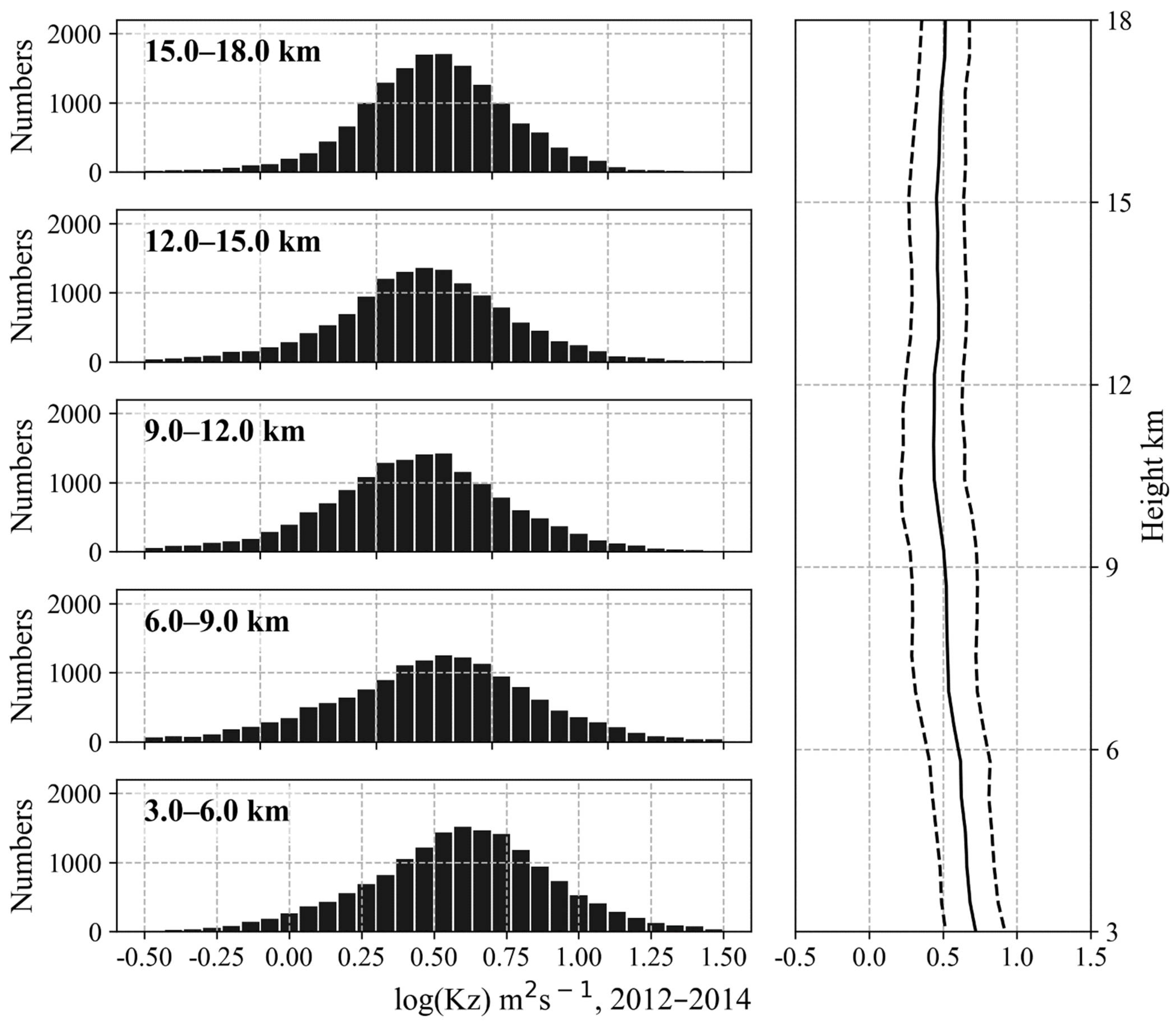
Figure 3 shows the distribution of
logarithmic values and the median profile and the upper and lower quartile profiles in the range of 3–18 km every 3 km. The
distribution is from 10
0 to 10
1 m
2 s
−1, spanning an order of magnitude, and the shape conforms to the Gaussian distribution. The median of
is distributed from 10
4 to 10
0.75 m
2 s
−1, and the upper and lower quartiles of log(
) are approximately between the median values ±0.25.
decreases from 10
0.75 m
2 s
−3 at 3 km to 10
0.5 m
2 s
−1 at 10 km. From 10 to 18 km,
changes very little with height, and the value is about 10
0.5 m
2 s
−1.
3.2. Seasonal Variation of Turbulence Parameters with Height from the Ground
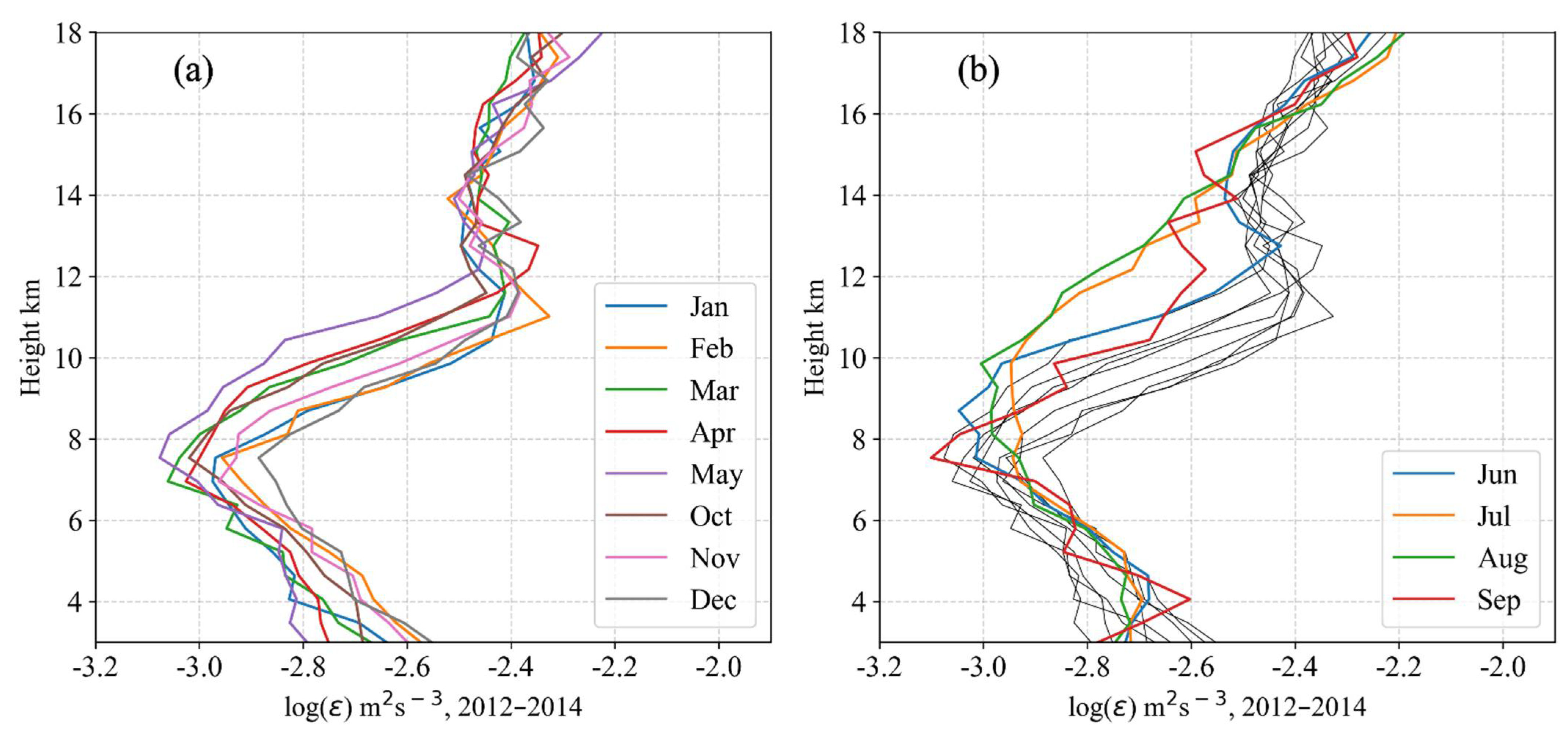
This section uses the Beijing MST radar observational data from 2012 to 2014 to analyze the variational characteristics of turbulence parameters in each month with height from the ground.
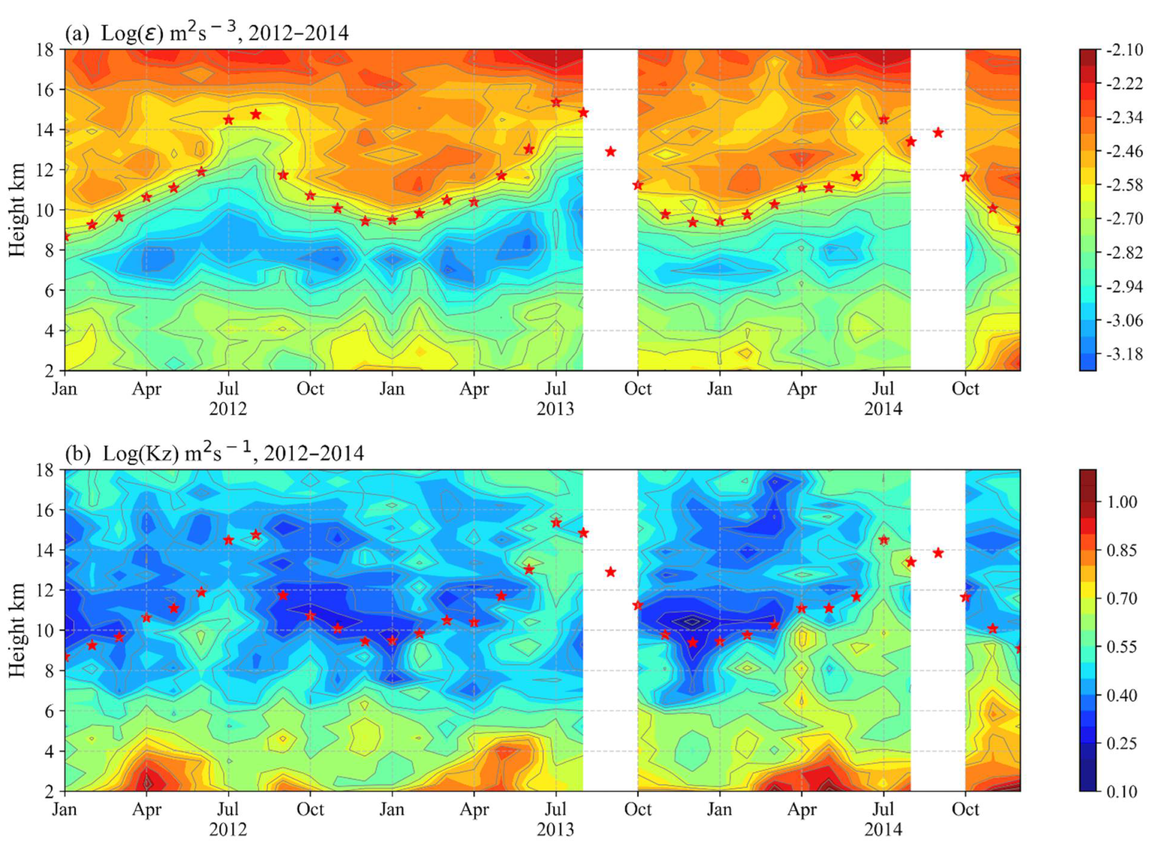
The value of
ε in the stratosphere is higher than in the troposphere, as shown in
Figure 4a. The median value of
ε in each month is distributed from 10
−3.2 to 10
−2.1 m
2 s
−3. There is a minimum value of
ε in the troposphere. The contours clearly show that the lower boundary of the small-value layer has no apparent monthly difference, while the upper boundary increases (decreases) with the increase (decrease) in the tropopause height. The tropopause height is about 15 km in July and August, and the lowest height of the tropopause is about 9 km in December and January. Furthermore, the center position of this minimum layer is about 7.5 km from October to the following May, and the height is about 10 km in July and August. June and September are more likely the transitional months.
In the height region below 7.5 km, below the minimum value of ε, ε decreases with height from the ground in each month. Additionally, the density of the contours indicates that the rate of decline of ε has no obvious monthly difference in the height region below 7.5 km. The highest increasing rate is at a few kilometers above and below the tropopause. However, the density of the contours in July and August is weaker than in other months, which shows that the increasing rate in the tropopause in July and August is lower than in other months.
In the range from the tropopause to 14 km, the value of ε has a peak layer from October to the following May. The peak layer starts in September and disappears in June of the following year. In July and August in Beijing, this layer disappears due to the tropopause rising to over 14 km. In the range of 15–18 km in Beijing, the value of ε from May to October is significantly larger than in other months.
The
of the troposphere is greater than the value of the stratosphere and has a rougher profile in each month compared with
ε, as shown in
Figure 4b. The median value of
in each month is distributed between 10
0.1 and 10
1.0 m
2 s
−1. In the range of 2–4 km from the ground, there is a large value from March to May and from September to October. Additionally, the value is larger and the thickness of this large-value layer is thicker from March to May.
At 1 km above the tropopause, has a minimum value in each month except July and August, and the distance from the ground is about 11 km. In July and August, the tropopause rises and this minimum layer disappears. At the height of several kilometers below the tropopause, there is an extreme-value zone for , and the height of the large-value zone rises as the tropopause height rises, which leads to having no minimum zone around 10–11 km in July and August. The upper boundary of the range in the decline in height of in the troposphere is about 7.5 km in July and August. However, this upper boundary is at 1 km above the tropopause (the height of the minimum value) in other months. Therefore, in July and August, in the height range from 7.5 km to 15 km, the characteristics of changing with height are different from the other months.
The monthly variations in the vertical structure of indicate that in the mid–lower troposphere and the region around the tropopause, there are apparent differences in the variation. When discussing the seasonal variation characteristics of the vertical structure of , it is necessary to consider the suitability of seasonal divisions in different atmospheric layers.
4. Discussion
4.1. Comparison of Atmospheric Turbulence Parameters and Atmospheric Stability
Unstable airflow will become or maintain turbulent flow and stable airflow will become or maintain laminar flow. This section analyzes the seasonal changes of turbulence parameters in the troposphere–lower stratosphere over Beijing from the perspective of atmospheric stability. Many factors determine the atmospheric stability, and these influencing factors can be understood as items in the turbulent kinetic energy (TKE) budget equation. There is static stability that is a measure of buoyancy convection capacity, and the BV frequency can represent the static stability of the atmosphere. Static means no movement. That is, the static stability does not consider the influence of wind. However, there is wind shear in the actual atmosphere, and even if the atmosphere is stable, wind shear can produce mechanical turbulence. When considering the terms of the TKE budget equation, to effectively approximate the simplification, researchers define the dimensionless ratio of the buoyancy generation term and the mechanical generation term as the flux Richardson number Rf.
The Rf includes turbulence-related factors. We can only use Rf to determine whether the turbulent flow can become a laminar flow, but we cannot judge whether the laminar flow can become turbulent. According to K theory, the gradient is directly proportional to the turbulence correlation. Therefore, if the gradient replaces the turbulence correlation in Rf, a new ratio can be obtained, called the gradient Richardson number
. The formula is as follows:
where
g is the gravitational acceleration,
is the potential temperature, and
is the square value of the horizontal wind vertical shear. The B-V frequency can be calculated using the formula
.
When Rf > 1, the buoyancy term is greater than the mechanical term, and the atmosphere will maintain or become a stable laminar flow. When Rf < 1, the atmosphere is considered unstable, and the atmosphere maintains or becomes turbulent. However, for Ri, when Ri < Rd, the atmosphere is unstable, and when Ri > Rt the atmosphere is considered stable. The value of Rt is 1, and the value of Rd is in the range of 0.22–0.25. This paper takes Rd = 0.25.
Based on the observational data of Beijing MST radar from 2012 to 2014, this section compares the median logarithmic values of turbulence parameters with the values of the atmospheric stability in each month. The atmospheric stabilities used in this study include atmospheric static stability, B-V frequency N, atmospheric dynamic stability, and gradient Richardson number Ri.
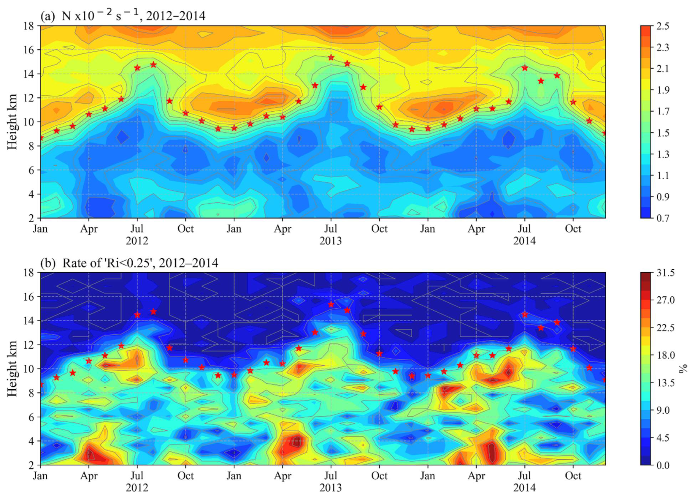
Figure 5 shows the monthly median values of B-V and the percentage of Ri < 0.25 at each height from 2 to 18 km.
In the height region of 2–18 km in Beijing, the seasonal variation characteristics of
ε and N are in good agreement.
Section 3.2 shows that from the tropopause to 16 km, there is an apparent large-value layer for
ε from October to the following May. June and September are the transition months for this high-value layer. The values of N also have the same seasonal characteristics, as shown in
Figure 5a. From October to the following May, the contours of
ε are very dense at the tropopause. N also has the same characteristics at the tropopause, which shows that the large gradient of
ε at the tropopause is related to N. The values of
ε and N have a corresponding excellent relationship between the large values and the small values. Function (3) also shows that
ε has a positive correlation with N and turbulence intensity. However, this section mainly compares the seasonal characteristics of Beijing’s turbulence parameters and atmospheric stability at mid-high latitudes.
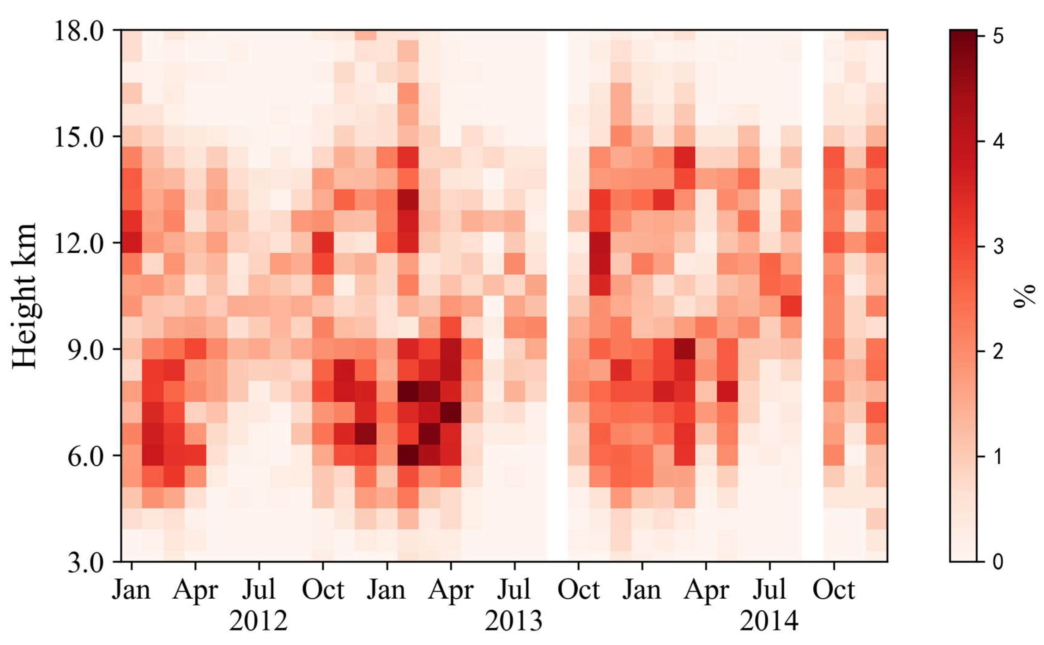
In the height region below the tropopause in Beijing, has a corresponding good relationship with the large values of the percentage of Ri < 0.25. Within the range of 2–4 km, the percentage of Ri < 0.25 and the values of both have a large-value layer from March to May and from September to October. From March to May, the percentage of Ri < 0.25 is greater than in September and October, and the upper boundary of this large value layer is significantly higher than from September and October. In the height region of 2–3 km below the tropopause, the large value of the percentage of Ri < 0.25 corresponds to the large value of .
This study also finds that the seasonal variation of atmospheric turbulence parameters has significant differences in different atmospheric layers. When considering the beginning and end months of a season, the division points of different layers might be different. For example, the values of ε and N have noticeable seasonal changes from the tropopause to 16 km in Beijing. However, the values have no obvious seasonal variation in some height ranges, mainly in the range of 6–8 km and the heights below 6 km. For and the percentage of Ri < 0.25, the values have different seasonal variation in different atmospheric layers—mainly the heights below 4 km and the range from 8 km to the tropopause. These characteristics show that even when studying the seasonal characteristics of atmospheric turbulence parameters at different levels at the same station, it is necessary to pay attention to the difference between the beginning and end months of different seasons. This section mainly discusses and compares the seasonal characteristics of atmospheric turbulence parameters and atmospheric stability in mid-high latitude regions, but the causes of these characteristics need to be further investigated.
4.2. Correlation Analysis of Turbulence Parameters and Atmospheric Stability/Turbulence Intensity
Section 4.1 shows that the turbulence parameters and the atmospheric static/dynamic stability have a good relationship at some altitudes. At the same time, the turbulence intensity (turbulence spectrum width
) is also one of factors influencing turbulence parameters (Formulae 3 and 4). Therefore, this section uses the Pearson correlation coefficient to measure the linear correlation between turbulence parameters and atmospheric stability, and the linear correlation between turbulence parameters and turbulence intensity, with the significance tested with a two-sided test. When the two-sided p-value is less than 0.05, it is considered to have passed the significance test with a 95% confidence interval. Otherwise, it is deemed to have failed the significance test. The results are shown in
Figure 6.
Figure 6a is a filled contour plot of the correlation coefficients of
ε and N in each month and at each height.
Figure 6b shows the correlation coefficients of
ε and N as well as
and the probability of Ri < 0.25 in each month and at each height.
ε and N have an apparent positive correlation below 14 km (consistent with the conclusion of
Section 4.1), and the correlation coefficient is about 0.5–0.9. However, the correlation between
ε and N did not pass the significance test in the range of 14–17 km.
ε and
have a noticeable positive correlation in the 2–18 km range, and the correlation coefficient is greater than 0.5.
ε and the monthly frequency of Ri < 0.25 have a significant negative correlation in the height range of 10–12 km, and the correlation coefficient is between −0.7 and −0.8. The above statistical results show that in the height ranges of 2–4 km and 9–13 km, the
ε may be affected by the stability of the atmosphere and the intensity of turbulence. In the range of 4–9 km, the contribution of atmospheric dynamic stability to
ε may be weak. In the range of 14–17 km, the intensity of turbulence may be the main factor affecting the
ε.
Figure 6c presents the statistical results of the correlation coefficient between
and atmospheric stability and turbulence intensity at various heights. The results show that at 6–8 km and above 15 km,
and
have a significant positive correlation with a correlation coefficient between 0.7 and 0.9. However, the correlation with atmospheric stability parameters failed the significance test. In other altitude ranges,
mainly has a significant positive (negative) correlation with the monthly occurrence probability of Ri < 0.25 (N), especially from 2–4 km and 9–11 km, and the correlation coefficient is around 0.75 (−0.75). At about 14 km, the absolute values of the correlation coefficients between
and N,
and the monthly frequency of Ri < 0.25 are all about 0.7. The above results show that the main factor influencing
is the turbulence intensity at 6–8 km and above 15 km. In the lower troposphere (2–4 km) and near the tropopause (9–11 km), atmospheric stability has a more significant impact on
, which may be related to the sharp change in atmospheric stability within this height range. At about 14 km, the atmospheric stability and turbulence intensity significantly affect the
.
Based on the above analysis, the turbulence intensity above 15 km is the main factor affecting the ε and . Therefore, it is vital to detect and study the stratospheric turbulence intensity. In this regard, MST radar can play an important role. The increase of turbulence intensity above 15 km may be related to gravity wave activity and its breaking, and further research should be carried out.
4.3. Increasing Rate of in the Tropopause
The results in
Section 3.2 show that it is inapposite to analyze the seasonal characteristics of turbulence parameters with a simple four-season classification in Beijing. The monthly averaged profiles of
ε show that January–May and October–December (or October to the following May) is significantly different from July and August, while June and September are transition months, as shown in
Figure 7. In the height range of 6–8 km,
ε has a minimum value and the values of
ε change sharply from October to the following May in the range of a few kilometers above and below the height of minimum
ε. However, the change in
ε values at the height of the minimum-value layer is relatively gentle in July and August. At the height of about 12 km,
ε has a maximum value from October to the following May, which is the peak value of
ε from the tropopause to 14 km, as mentioned in
Section 3.2. However,
ε has no such maximum value in July and August.
In the range of 2–4 km, the profiles of ε have seasonal variations. From October to the following May, ε decreases with the same rate from 2 to 7.5 km, but tends to increase with height at 2–4 km from June to September. In the range of 6–8 km, the structure of ε in June is the same as in July and August, while the structure in June is the same as from October to the following May at the height of about 12 km. The structure of ε in September is opposite to that in June. Therefore, this study defines June and September as transition months when we discuss the seasonal variations of ε.
In July and August, the profiles of
ε have no noticeable difference from 2–18 km. From October to the following May, the values of
ε have a monthly difference in the range of 2–12 km, while the trends of the monthly mean profiles are almost the same.
ε has a significant increase in the range of 7–11 km from October to the following May, as shown in
Figure 7a.
Section 3.2 also shows that
ε has the most significant increase at the tropopause height. Some studies [
13,
20] have pointed out that turbulence parameters have sharp changes in the tropopause. Therefore, we reconstructed a new dataset with the reference height of the tropopause. Each profile of the new dataset varies with the height of the tropopause.
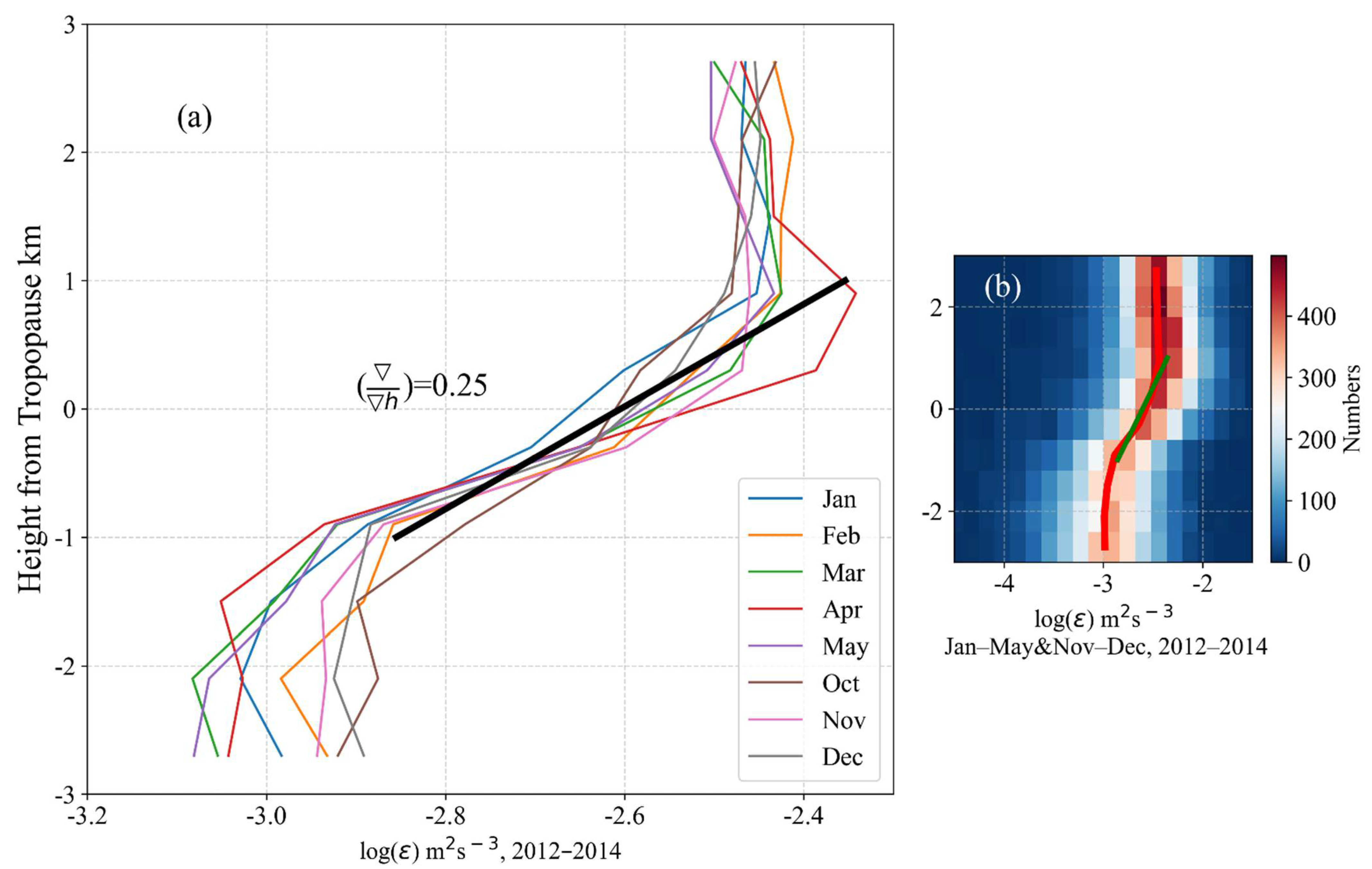
The monthly mean profiles of
ε changing with the tropopause height are shown in
Figure 8a. From October to the following May, there is no obvious monthly difference at 1 km above and below the tropopause. In the range of −1 to +1 km from the tropopause, the increasing linear rate of log(
ε) is 0.25 m
2 s
−3 km
−1. The linear rate is calculated by linear regression using all scatter points in the range of −1 to +1 km from the tropopause, and the frequency distribution of the points is shown in
Figure 8b. The red curve in
Figure 8b is the mean value of
ε at each height, and the profiles of
ε in each month (
Figure 8a) are also obtained by analyzing the frequency distribution. There are two reasons for using the average value here. First, the height of the tropopause is calculated using a sounding temperature profile with a resolution of 50 m. Therefore, the height of each profile in the new dataset is different. The new datasets need to be interpolated when analyzing the statistical characteristics of the turbulent parameters. Given that, it is more appropriate to use the monthly averaged profiles. Second, the amount of data for three years is enough to ensure that the average results can represent the statistical characteristics of turbulence parameters.
From October to the following May, in the height regions about 1 km above and below the tropopause, there is no significant difference in the profile of ε with the height from the tropopause, except in April, when the values of ε in the 0 to +1 km layer above the tropopause are stronger. Therefore, the tropopause is a significant reference height for studying turbulence parameters. The trend and rate of change of ε with height from the ground are the same in these months. Therefore, if the height of the tropopause is known, it would be likely that the monthly average profile of turbulence parameters changing with height from the ground can be obtained. However, whether this feature can be applied in specific cases requires further verification through a large number of cases.
5. Conclusions
This study used three years of data observed by Beijing’s MST radar from 2012 to 2014 to calculate the turbulent parameters (ε and , mainly) in the troposphere–lower stratosphere by using the spectral width method. This paper presents the characteristics of turbulence parameters changing with height in each month and season; plus, comparison of the seasonal variations between turbulence parameters and atmospheric stability (N and Ri) was also conducted. The conclusions are as follows:
- 1.
The
ε in Beijing is distributed from 10
−4 to 10
−1.5 m
2 s
−3, spanning 2.5 orders of magnitude, and the shape conforms to the Gaussian distribution. The median values of
ε are from 10
−3 to 10
−2.5 m
2 s
−3.
is distributed between 10
0 and 10
1 m
2 s
−1, spanning an order of magnitude. The median values of
are distributed between 10
0.4 and 10
0.75 m
2 s
−1. The turbulence parameters of Beijing MST radar show inconsistency with some of the results of previous studies, but are more consistent with the results of Harrow radar (42.04° N, 82.89° W) which is located at the nearest latitude compared with the Beijing MST radar site [
13].
- 2.
Comparison of turbulence parameters and the monthly variation characteristics of atmospheric stability with altitude showed that the vertical structure of N and ε in the height range of 2–18 km has good consistency. In the range of 2–14 km, the Pearson correlation coefficient is between 0.5 and 0.9. From the tropopause to 14 km in Beijing, the values of ε and N both have a peak layer from October to the following May.
- 3.
The frequency of Ri < 0.25 is in good agreement with the vertical structure of in the region below the tropopause. Within the height range of 2–4 km from the ground in Beijing, and the percentage of Ri < 0.25 have a significant correlation, with a Pearson correlation coefficient of about 0.75, and both have a large-value layer in March–May and September–October.
It is worth noting that the results of this study show that not only are the seasonal divisions of different regions different, but the seasonal divisions of different atmospheric layers in the same region are also different. The statistical results of ε indicate that June and September are the transition months in Beijing, and the vertical structure of ε is one type from October to the following May, and another type in July and August. However, the statistical results of show that this seasonal classification is unsuitable in the height range of 2–4 km, while this seasonal classification is suitable for at heights above 4 km. The seasonal variation of the vertical structure of is more complex, which indicates that there are specific differences in the beginning and end months of different seasons at different levels of the atmosphere.
This paper gives the statistical results of turbulence parameters, but how the turbulence parameters change during synoptic processes needs to be further investigated. For example, the correlation analysis in this paper shows that the turbulence parameters above 15 km may be mainly affected by the turbulence intensity; the results of Khoma et al. [
15] show that the seasonal characteristics of turbulence parameters are related to gravity waves in the Antarctic stratosphere; and Li et al. [
14] calculated
ε under different Ri, and the results showed that the median values of
ε when Ri < 1 is 3.2 times that of when Ri > 1. From October to the following May, in the height layer of 1 km above and below the tropopause, there is no apparent seasonal difference in the monthly average profile of
ε. Additionally, log(
ε) increases sharply with a rate of 0.25 m
2 s
−3 km
−1, derived by linear regression. This vertical structure of
ε indicates that the tropopause is a suitable reference height for studying turbulence parameters. Although some studies have used the tropopause as the reference height to analyze the statistical characteristics of turbulence parameters [
20], [
13], a large number of case studies are still needed to discuss the role of the tropopause in studying the vertical structure of turbulence parameters.


