Abstract
The ionospheric plasma density irregularities are known to play a role in the propagation of electromagnetic signals and to be one of the most important sources of disturbance for the Global Navigation Satellite System, being responsible for degradation and, sometimes, interruptions of the signals received by the system. In the equatorial ionospheric F region, these plasma density irregularities, known as plasma bubbles, find the suitable conditions for their development during post-sunset hours. In recent years, important features of plasma bubbles such as their dependence on latitude, longitude, and solar and geomagnetic activities have been inferred indirectly using their magnetic signatures. Here, we study the scaling properties of both the electron density and the magnetic field inside the plasma bubbles using measurements on board the Swarm A satellite from 1 April 2014 to 31 January 2016. We show that the spectral features of plasma irregularities cannot be directly inferred from their magnetic signatures. A relation more complex than the linear one is necessary to properly describe the role played by the evolution of plasma bubbles with local time and by the development of turbulent phenomena.
1. Introduction
One of the most interesting features of the equatorial ionospheric F region is the existence of plasma density irregularities, which find the suitable conditions for their development during post-sunset hours [1]. In the last few years, different terminologies have been used to term the equatorial ionospheric irregularities. Often, these are identified as equatorial spread-F, in virtue of the spread of the experimental trace either in frequency or in amplitude affecting the ionosonde observations, which is the marking of the existence of electron density irregularities in the reflecting layer (e.g., Booker and Wells [2]). With the advent of in situ satellite observations, they started using terms such as “depletions”, “bite-outs,” or “plasma holes”, because the irregularities were recorded mostly at locations where the electron density is depleted with respect to the background ionosphere (e.g., McClure et al. [3], Dyson and Benson [4]). Then, terms such as “plumes” or “wedges” appeared to characterize the morphology of turbulent regions and the development of such irregularities, as observed by radars (e.g., Scannapieco and Ossakow [5], Woodman and La Hoz [6]). In the last few decades, to identify the generation process of these irregularities, the term “bubble” has taken hold more and more (e.g., Burke [7]). It is worth noting that recent studies (e.g., Kil et al. [8]) introduced also the expression “plasma depletion shell” to highlight the three-dimensional structure of bubbles. The formation of these irregularities is recognized to be driven by the Rayleigh–Taylor instability mechanism [6,9,10] that generates in the ionosphere a situation similar to that occurring when a heavy fluid flows over a lighter one. The absence of sunlight, which leads to a different rate of recombination in the ionospheric layers, causes a density gradient between the upper and lower ionospheric F region with a plasma density in the upper F region higher than in the lower one. Such steep vertical density gradients realize the conditions for the growth of the Rayleigh–Taylor instability. These plasma density irregularities expand vertically and successively move along the magnetic field lines on each side of the geomagnetic equator. Typically, they also drifted eastward from vertical polarization electric fields associated with zonal neutral winds in the F region.
The result is the formation of magnetic field-aligned plasma-depleted regions, which are usually known as equatorial plasma bubbles. They are unstable to plasma density perturbations and polarization electric fields so that secondary irregularities can be generated, which are mainly the result of cascading processes. Nowadays, many important characteristics of these irregularities are known. They have different scale sizes, from hundreds of kilometers down to a few decameters [11,12], are mainly observed within a narrow band of magnetic latitude [9], are observable in a wide range of altitudes [6,9] up to around km [13,14,15], and their spatial and temporal distributions are strongly controlled by various geophysical parameters such as solar [16] and geomagnetic activity [17], season [16,18], local time, and longitude [8,19,20,21]. What drives the scientific community to investigate the plasma density irregularities is the knowledge of their role in the propagation of electromagnetic signals. They can be responsible for the disturbance of radio waves and are one of the most important sources of disturbance for the Global Navigation Satellite System (GNSS) signal. Indeed, in the worst case, plasma density irregularities can cause a loss of lock event, a condition for which a GNSS receiver can no longer track the signal sent by the satellite, with a consequent degradation of the positioning accuracy. In the last few years, the relevance of the GNSS in our society has substantially increased, as many critical infrastructures and economies are dependent on the positioning, navigation, and timing services of GNSS, so that our society is nowadays vulnerable to damages due to the malfunction of these systems. For this reason, one of the research priorities in the space weather community is to improve the knowledge of these plasma density irregularities, trying to better understand their features and generation mechanisms.
An interesting aspect of these irregularities, which requires more study, is their possible turbulent nature. Indeed, the equatorial ionosphere has proper physical conditions for the establishment of a fully developed turbulence [22,23]. Through numerical simulations, it has been possible to reproduce the ionospheric irregularities and study the corresponding dynamics under collisional and inertial regime flows [24,25]. It has been found that the plasma irregularities may be characterized by energy spectra with slopes ranging between and associated with the occurrence of energy and/or enstrophy cascades, respectively [26,27]. Over the years, these numerical models have been improved trying to describe the ionospheric two-dimensional plasma turbulence in a more realistic way. It has been found that after sunset, at apex heights between 600 and 1000 km, large-scale irregularities present a dynamics typical of inertial regime flow [28] and that although the foundations of the Kraichnan’s theory could be undetermined in the topside equatorial ionospheric F region, the numerical simulation results seem to confirm the probable existence of large plasma density irregularities. These are characterized by velocity fluctuation spectra following power laws with spectral indices similar to those predicted for energy and enstrophy cascades in two-dimensional turbulent flows [23]. In the last twenty years, thanks essentially to the rapid increase in the performance of computers, it has been possible to improve the models describing the evolution of plasma depletions. Thus, new models capable of reproducing the three-dimensional turbulent structures of equatorial plasma bubbles with high spatial and temporal resolutions have been developed (see for example Yokoyama et al. [29], Yokoyama [30]). The results of such simulations confirm observations of plasma density data recorded, for example, on board DE-2 satellite. In this case, it has been found that plasma density is characterized by an energy spectrum with a slope around for scale sizes larger than 1 km in all regions characterized by strong plasma density irregularities [28]. Nowadays, the numerical simulations have become useful tools both to study the plasma bubbles and their nonlinear evolution, and to understand some of their features, which cannot be fully understood from theoretical predictions. Therefore, it is extremely important to combine the numerical simulation results with real observations.
In order to detect and characterize plasma density irregularities, different methods, approaches, instruments, and data can be used such as, for example, ionosondes, airglow imager, coherent/incoherent scatter radars [31], as well as Global Positioning System (GPS) Total Electron Content (TEC) [32,33] in the topside ionosphere. The ground-based observations are mostly fixed in a single location and cannot give the spatial variations of plasma density irregularities in a large area. Conversely, observations from Low Earth Orbit (LEO) satellites such as for example DMSP (Defense Meteorological Satellite Program), ROCSAT-1 (Republic of China Satellite), C/NOFS (Communications/Navigation Outage Forecasting System), and COSMIC (Constellation Observing System for Meteorology, Ionosphere, and Climate) permitted climatology studies and provided the latitude-local time distributions of plasma density irregularities. The recently launched Global-scale Observation of Limb and Disk (GOLD) mission, which is located at a geo-stationary orbit, seems to be a promising mission to study bubbles, offering the opportunity to observe the Earth’s complete disk continuously from the geostationary orbit [34,35]. A different method for the detection of ionospheric irregularities based on the diamagnetic effect was suggested a few years ago. Plasma density irregularities are indeed associated with magnetic field perturbations [36,37] that can be used as a proxy for plasma irregularities. There are different ways to describe the so-called diamagnetic effect but, perhaps, the easiest one is to consider that the sum of magnetic and plasma pressures has to be constant in a quasi-stationary state. This means that when the plasma pressure is reduced, the magnetic pressure and consequently the magnetic field strength must increase. The equatorial plasma bubbles identify regions of reduced plasma density; consequently, they have to be characterized by a magnetic field strength higher than the ambient one. That was confirmed using simultaneous observations of magnetic field and electron density recorded by the CHAllenging Minisatellite Payload (CHAMP) satellite. These measurements revealed the increase of a few nT in the main field intensity inside the plasma density depletions [38] Park et al. [39] quantitatively investigated the actual balance between plasma and magnetic pressures within the plasma bubbles, showing that a dominant part of the magnetic pressure change could be explained in term of plasma density change under specific assumptions. Based on the high correlation between the variations of plasma density and those associated with magnetic field strength, an extensive survey of magnetic signatures related to plasma density irregularities was used for statistical studies [15,40,41] devoted to the analysis of the global distribution of equatorial plasma irregularities in the topside ionosphere. These studies revealed features of the magnetic signatures that closely reflected those of the plasma bubbles previously obtained using different methods as GPS scintillation [19], in situ plasma density measurements [42,43], and radio wave propagation [44]. Furthermore, magnetic field measurements recorded on board the CHAMP satellite with different time resolution (50 Hz and 1 Hz) permitted addressing some properties of the plasma density irregularities related to their different spatial sizes. Evidently, these results do not reflect directly the features of plasma depletions but their associated magnetic signatures. However, the features obtained using the magnetic signatures of the plasma depletions are consistent with those obtained by directly using the electron density measurements. For this reason, the diamagnetic effect, as an indirect way of sampling plasma density structures, can be extremely useful in studying plasma irregularities.
While it is correct to assume that some plasma bubbles features can be inferred using the corresponding magnetic signatures, the assumption that plasma bubbles scaling properties can be inferred using the associated magnetic field scaling properties may be not necessarily correct as well. The purpose of this study is to understand if the hypothesis of a linear relation between the scaling properties of the electron density and of the magnetic field is valid. So, needless to say, the clarification of this point is of crucial importance.
2. Data Description
To investigate the scaling features of the electron density irregularities and of their magnetic signatures at low latitude, we use measurements on board the Swarm A satellite during its near-polar orbit around the Earth at an altitude of approximately 460 km [45]. Swarm A is one of the satellites constellation launched by ESA for Earth observation. Specifically, the ESA mission consists of three identical satellites named Alpha, Bravo, and Charlie (A, B, and C), which were launched on 22 November 2013 into a near-polar orbit. Swarm A and C fly side-by-side at an altitude of 462 km (initial altitude) and at an inclination angle of 87.35°, whereas Swarm B flies at a higher orbit of 511 km (initial altitude) and at an inclination angle of 87.75°.
We consider measurements collected from 1 April 2014 to 31 January 2016 at low and mid latitudes () under conditions of high solar activity. It is known indeed that the equatorial plasma bubbles occur mainly during periods characterized by high extreme ultraviolet solar flux [41]. In the selected time interval, the value of the solar radio flux index (F10.7) is equal to sfu. This is not an extremely high value for the solar activity, but the selected period, which covers a part of the descending phase of Solar Cycle 24, is the only period of moderate/high solar activity during which Swarm is flying. Electron density and magnetic field vector data at a rate of 1 Hz are selected from the ESA dissemination server (http://earth.esa.int/swarm accessed on 12 February 2022). To highlight the magnetic signatures associated with plasma bubbles, we remove from the magnetic field measurements the contribution due to the magnetic field of internal origin, as modeled by CHAOS-6 [46]. CHAOS-6 is the latest generation of the CHAOS series of global high-resolution geomagnetic field models, which spans a period between 1997 and 2016. It is derived primarily from magnetic satellite data (Swarm, CHAMP, Ørsted, and SAC-C), although ground-based activity indices and observatory monthly means are also used. It is able to model the dominating core field, the crustal field, and the magnetic fields from large-scale magnetospheric currents, but there is no explicit representation of the ionospheric field or fields due to magnetosphere—ionosphere coupling currents. One of the applications of this model is the removal from the observed magnetic field of the large contributions from the prime sources when the weaker effects such as ionospheric currents, plasma irregularities, or even ocean tidal motions want to be investigated. We use the CHAOS-6 package to compute the geomagnetic field of internal origin, which is successively subtracted to the magnetic field observed by Swarm. Lastly, we focus on the 18:00–24:00 local time (LT) sector and select periods characterized by low/moderate geomagnetic activity. To select these periods, we used the index, which is designed to measure the solar particle radiation through its magnetic effects, and today, it is considered a proxy for the energy input from the solar wind to Earth. It is a global geomagnetic activity index based on 3-hour measurements from ground-based magnetometers around the world. The index ranges from 0 to 9, where a value of 0 means that the geomagnetic activity is absent, and a value of 9 means that an extreme geomagnetic storming is occurring. Data are distributed by GFZ (Helmholtz Centre Potsdam) [47] and they are redistributed by various data centers and databases. To select periods characterized by low/moderate geomagnetic activity, we consider all those time intervals characterized by . According to previous results [40], the probability of observing plasma bubbles is maximum under these conditions.
To select the plasma bubbles events, we use the Swarm Level-2 Ionospheric Bubble Index (IBI) product, which was evaluated using plasma density and magnetic field data with a cadence of 1 Hz. A full description of the data file and explanations regarding the IBI data can be found in the L2-IBI product description file (https://earth.esa.int/eogateway/documents/20142/37627/Swarm-Level-2-IBI-product-description.pdf/3e9f6c3a-1ffc-ea53-0161-a18b63f90c6f, accessed on 13 February 2022). This product is composed of three parameters: Bubble Index, Bubble Probability, and Bubble Flag. The Bubble Index can assume three different values: 1, when the analyzed data are affected by a plasma bubble, 0 when there is not a plasma bubble, and −1 when conditions do not allow unequivocally identifying a plasma bubble in the data [48]. Furthermore, when IBI = 1, there is an additional flag, the Bubble Flag (BF), indicating the quality of plasma bubbles detection that is related to exceeding a certain probability threshold. When BF = 1, we are in the presence of a high correlation between plasma density depletion and magnetic field signature. Here, we chose the condition IBI = 1 and BF = 1 to identify the plasma bubbles. However, we note that this automatic detection algorithm cannot distinguish equatorial plasma bubbles from plasma blobs, which are localized plasma density enhancements. This means that the events identified by the L2-IBI processor can contain also blob events. However, the occurrence probability of equatorial plasma bubbles is significantly higher than that of blobs mainly during solar maximum years.
3. Method and Data Analysis
The scaling features of the electron density and magnetic field at different temporal scales are evaluated using the so-called generalized -order structure function, namely . For a signal , is given by the following equation:
where t is the time, is the time delay, and stands for a statistical average. When has a power-law behavior as a function of :
the analyzed signal is characterized by a scale invariance, and is the so-called order scaling exponent, which defines the scaling nature of the increments of the signal . A signal possesses a global scale-invariance if ; that is, it is a linear function of the order q. Conversely, a signal is defined as multifractal, that is, it has a local scale-invariance, if is a nonlinear convex function of q. Here, we investigate the second-order scaling exponent, , which is related to the power spectral density (PSD) exponent, (PSD ), via the following relation:
The use of the structure function analysis, rather than the standard Fourier analysis, as a method to detect scaling features is motivated by the fact that the analysis of scaling/spectral features in the real time space, using signal increments, is less affected by the choice of a specific decomposition basis, as it is instead the case for the Fourier analysis. Furthermore, being geophysical signals, such as magnetic field and electron density fluctuations in the ionosphere, generally characterized by power-law spectra, i.e., , with spectral exponents ranging between 1 and 3, one deals with nonstationary signals with stationary increments [49]. In this case, the Fourier analysis, which requires stationarity, might produce unreliable results especially when evaluating spectral properties over short time intervals. Conversely, the structure function analysis works with signal increments that are expected to be nearly stationary, and thus, the corresponding results over short time windows/intervals are more reliable. Furthermore, the structure function analysis is a companion method that is widely used in the framework of turbulence-related studies.
The measurements collected by instruments on board a satellite require some precautions to be correctly used. The satellite crosses regions characterized by different physical processes, which change in space and time. Consequently, the collected measurements, such as in our case electron density and magnetic field strength, present properties with a local character. The scaling properties of these real-time series also acquire a local character, and it is necessary to apply methods of analysis capable of evaluating their local scaling features describing the different regions explored by the satellite. The structure function approach allows doing this. Among the different methods to evaluate the structure functions, here, we apply the local detrended structure function analysis (DSFA) method discussed in De Michelis et al. [50,51] and already successfully applied in a series of previous works showing results that are well in agreement with the present literature on the scaling and/or spectral features of turbulent fluctuations in the ionosphere. In detail, we apply the analysis on a moving window of points using a time series obtained from the original one after removing its linear trend, if present. This gives us the opportunity to remove from the initial signal all the possible large-scale variations that can affect a correct estimation of the scaling features. The choice of a moving window of 301 points is the result of an accurate series of test over a wide set of simulated multifractional Brownian motions [52,53,54], which are characterized by a local dependence (nonstationarity) of the scaling/spectral features. Indeed, this number of points is the right compromise to get an estimation of local scaling exponents sufficiently precise (with a typical error %), being 1 order of magnitude larger than the longest investigated timescale ( s). In each moving window, we evaluate the second-order structure functions associated with the electron density and magnetic field strength time series, respectively. These are evaluated for time delay values () ranging from 1 to 40 s, and the estimated second-order scaling exponents are associated with the position of the satellite at the center of the fixed window. We assume that the results obtained in the time domain are valid in the space domain too (see e.g., [55,56] and references therein). Thus, considering that the Swarm A orbital velocity is around 8 km/s, the results obtained in the time domain between 1 and 30 s are valid in the spatial domain between ∼8 and ∼250 km, i.e., where is the satellite velocity. We remark that the previous conversion between the timescale and the corresponding spatial scale is based on the assumption of the Taylor’s hypothesis according to which instantaneous spatial averages coincide with temporal averages calculated from the recorded signal. Given this hypothesis as valid, which can be applied for frozen turbulence, we assume that the temporal evolution of turbulent structures is longer than that required for the satellite to cross them [22,55,56,57]. Hence, by evaluating the scaling properties of the magnetic field strength and electronic density associated with the plasma bubbles, we can investigate the properties of these plasma density irregularities from both a magnetic and plasma point of view in a range of scales between some kilometers and a few hundred kilometers.
The structure function analysis is initially done on the entire time series of around points (22 months with a time resolution of 1 Hz) and only later, the scaling exponent values of the electron density () and magnetic field strength () associated with the occurrence of plasma bubbles are selected.
4. Results
Figure 1 reports a map of the values of the second-order structure function exponent, , which was obtained analyzing and inside the plasma bubbles. These two different parameters are characterized by similar values of , supporting the previous findings by Lühr et al. [15]. However, to look for any difference, we start by plotting in Figure 2 the corresponding histograms. The second-order structure function exponents range from 0.4 to 2 with the highest probability occurring at in both cases.
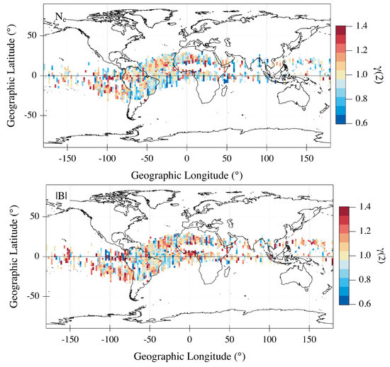
Figure 1.
Values of the second-order scaling exponent, , associated with electron density (top) and magnetic field strength (bottom) inside the plasma bubbles in the geographic latitude–longitude plane. Data are selected according to the following conditions: 18:00 ≤ LT≤ 24:00, geographic latitude, .
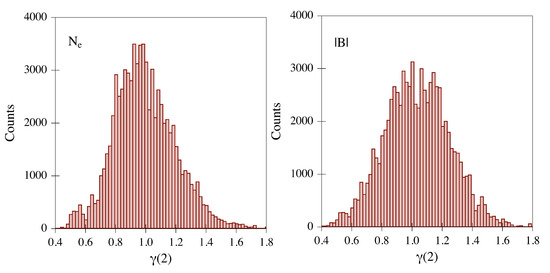
Figure 2.
Histograms of the second-order scaling exponent values associated with electron density (left) and magnetic field strength (right) inside the plasma bubbles, respectively. Data are selected according to the following conditions: 18:00 ≤ LT ≤ 24:00, geographic latitude, .
Taking into account the relation between the second-order scaling exponent and the Fourier power spectral density exponent (), we notice that the spectral features obtained in the case of electron density () are in agreement with previous results. For example, Livingston et al. [58] analyzing the spectra of electron density data recorded from the Atmospheric Explorer-E satellite (AE-E) in the interval 20:00–02:00 LT found a distribution of spectral slopes in the range between 1 and 3 centered around 1.9, which is a mean value that agrees with our results and is close to those of Dyson et al. [59], who used data recorded by the OGO satellite, Basu et al. [60], who analyzed AE-E measurements, and Le et al. [61], who analyzed ROCSAT-1 burst mode measurements at 1024 Hz sampling. Concerning the spectral scaling exponents obtained for the magnetic field strength, there are not many previous analyses with which to compare them. Lühr et al. [15] used magnetic field data recorded by CHAMP to investigate the spectral properties of the signal and found values of the spectral indices ranging between 1.4 and 2.6 with a peak around 1.9. Again, these results agree with ours. Although the mean values of the two distributions reported in Figure 2 are equal, their shapes are different, in which the distribution for is skewed. Indeed, the skewness values of distributions of and are and , respectively.
Figure 3 reports the values of the second-order structure function exponent obtained analyzing and inside the plasma bubbles according to QD magnetic latitude. For , the highest occurrence of is found for at a latitudinal distance from the equator of around in magnetic latitude in both hemispheres, while in the case of , the highest occurrence of is found for a value around 1 occurring always in the same regions. Thus, the peak of the highest occurrence of plasma bubbles is associated with a range of values that is smaller for than .
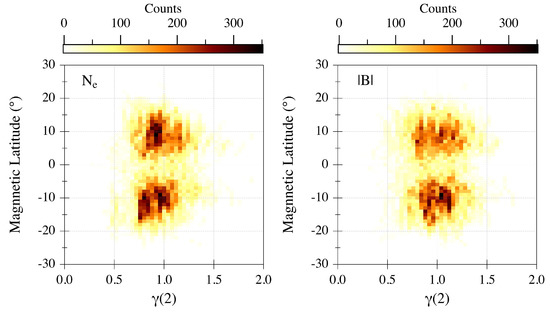
Figure 3.
Dependence on QD magnetic latitude of the second−order scaling exponent values associated with (left) and (right) inside the plasma bubbles.
To go into the observed differences between the two distributions, we repeat our analysis considering two-hour time intervals from 18:00 LT to 24:00 LT. Figure 4 reports the distribution of values relative to and in the three different selected time intervals. A double peak distribution of clearly appears analyzing the scaling properties of in the range 20:00 ≤ LT < 22:00. The distribution has one peak in the next local time interval (22:00 ≤ LT ≤ 24:00) and a rather flat shape in the previous one (18:00 ≤ LT < 20:00). In the case of values associated with , the data distribution has only one peak in the second and third local time intervals while a distribution with a rather flat shape appears in the first local time interval. The emergence of a bimodal distribution for the magnetic field exponent could be an indication of a non-unique relation between the scaling features of electron density and magnetic field fluctuations in plasma bubbles. Furthermore, as clearly shown in several works (see, e.g., [62]) (and references therein), in the second LT interval here considered, plasma bubbles are still evolving at Swarm altitude, so that the bimodality could be a reflection of the nonstationarity of the plasma bubble structures.
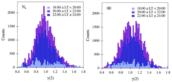
Figure 4.
Histograms of the second-order scaling exponent values associated with electron density (left) and magnetic field strength (right) inside the plasma bubbles, respectively. Data are selected according to the following conditions: 18:00 ≤ LT < 20:00 (light blue), 20:00 ≤ LT < 22:00 LT (blue) and 22:00 ≤ LT ≤ 24:00 (purple). In all cases, the geographic latitude is and .
To get more insights on the bimodal character of the distribution that appears, analyzing the scaling properties of inside the plasma bubbles between 20:00 LT and 22:00 LT, we check how the values of the two peaks are distributed in latitude and longitude. Taking into account that the two different populations are characterized by values of and , respectively, Figure 5 shows their distributions in the latitude–longitude plane. The two geographic distributions seem similar, although the values seem to prefer the areas closest to the equator. This feature is well highlighted on the bottom of Figure 5, where the values are sorted according to magnetic latitude. Here, the red line clearly shows how the plasma bubbles around the magnetic equator () are often characterized by a magnetic field strength with a second-order scaling exponent . The values of the scaling exponents of the magnetic field strength seem to depend on magnetic latitude at least during the hours following their formation. To better investigate this point, we report in the left panels of Figure 6 the joint probability distributions of values relative to () and () along with the mean values of exponent (white circles) for fixed at the three different selected two-hour time intervals. There is a large spreading of the observed distributions with most of the values concentrated around , which indicates that the relation between electron density and magnetic field scaling exponents can be assumed to be linear only in a zero-order approximation. However, looking at the trend of the mean values of fixed , we can realize how the relation between the two scaling indices significantly departs from a linear trend for at LT . This result suggests that a more complex relation might exist between plasma density and magnetic field variations. Furthermore, the departure from a linear relation increases with the midnight approaching. We can conjecture that the observed departure from linearity occurs when the fluctuations of the electron density show scaling features similar to those expected for convective turbulence, i.e., [63]. In the right panels of Figure 6, we report the conditioned probably distribution density functions of values for fixed . The observed distributions are multimodal, thus supporting the hypothesis that a linear relation between magnetic field intensity and plasma density spectral features has to be considered valid only on average being a very crude approximation. The multimodal structure of the observed distribution could also be the counterpart for different physical processes at the origin of the observed fluctuations, or it could be due to the role played by other physical quantities, such as for example the plasma temperature fluctuations, that could modify the relation between electron density and magnetic field second-order scaling exponents. Moreover, a very interesting result stands in the clear bimodal character of the distribution of the magnetic field exponent in the first LT sector. Indeed, there is not a one-to-one correspondence between the magnetic field exponent and that of the electron density fluctuations, i.e., . A possible explanation could be that, as shown in Gruzinov et al. [63], we are still in the early stage of a rising bubble so that the spectral features are still not stationary.
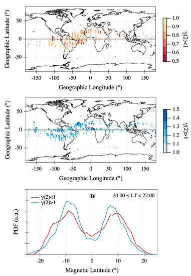
Figure 5.
Values of the second-order scaling exponent associated with magnetic field strength inside the plasma bubbles in the geographic latitude–longitude plane during the time interval 20:00 ≤ LT < 22:00 LT for and , respectively. On the bottom, the and values are sorted according to magnetic latitude.
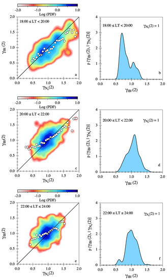
Figure 6.
On the left, the joint probability density functions of second-order scaling exponents for and for in the three different selected two-hour time intervals. White circles refer to the mean values of the magnetic field exponent at fixed electron density exponent values. The black line is the bisector line for which . On the right panels, the conditioned probability distribution density functions of values for fixed .
We conclude our analysis reporting in Figure 7 the probability density functions of the location of the plasma bubbles as a function of both the magnetic latitude and LT. These distributions suggest the tendency of plasma bubbles to move away from the equator as the time goes by. This could indicate that the plasma bubbles observed near the midnight sector have not been generated in that LT sector but could have been generated near sunset, have moved at high altitudes, and successively have started to descend in altitude, moving along the magnetic field lines. Indeed, the flux tube intersecting the 460 km Swarm A orbit at ∼10 magnetic latitude has an apex height around 600 km at the equator where the plasma bubbles are generated. This is a crucial point in the interpretation of the LT evolution of the scaling features of magnetic field and density fluctuations inside the plasma bubbles. It makes you understand how, moving away from the sunset, Swarm A crosses older plasma bubbles at locations where the turbulence had time to fully develop.
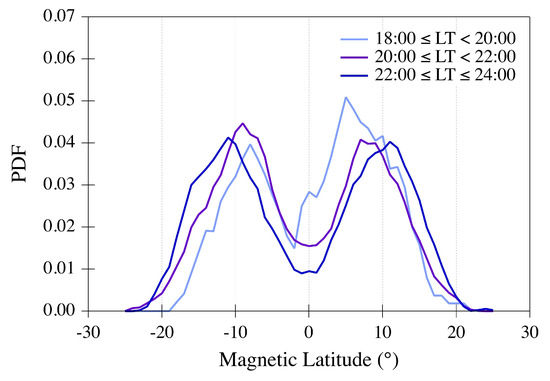
Figure 7.
Dependence on magnetic latitude and local time of location of the plasma bubbles.
5. Discussion
Our findings seem to suggest that a non-trivial linear relation exists between the spectral features of the plasma density and magnetic field in the plasma irregularities which depends on the local time and latitude. Actually, the fact that the magnetic field and electron density scaling properties are not simply linearly related is somehow expected. Usually, when we study the plasma bubbles dynamics, we start with a few assumptions.
First, following the derivation of the diamagnetic current in Alken et al. [64], i.e., considering the standard magnetohydrodynamic equations for a plasma in a steady-state configuration, that is, , and neglecting gravity, we can write that the plasma pressure force () is counter-balanced by the Lorentz force (), i.e.,
where is the ambient magnetic field. Combining Equation (4) with the Maxwell’s equation describing the Ampère’s circuital law in absence of displacement currents
where is the permeability of free space, we can write
The term on the left of Equation (8) is the sum of plasma pressure force and magnetic pressure one, while on the right, the term represents magnetic tension due to the curvature of the field lines. Taking into account that the plasma structures are much smaller than the geomagnetic field curvature radius, it is possible to assume a linear field line geometry. In this case, we can neglect the magnetic curvature term, , in the momentum balance so that a change in plasma pressure is, in first approximation, compensated by a change in the magnetic pressure (second assumption). Thus, according to Lühr et al. [37] and taking into account that , we can write that across the irregularity walls, the following relation holds:
where denotes a finite scale difference (i.e., the gradient in Equation (4) computed at the bubble intensity scales), is the Boltzmann constant, is the electron density, and and are electron and ion temperatures, respectively.
Third, considering that the strength of the ambient magnetic field is around four orders of magnitude greater than the magnetic field generated by the equatorial plasma bubbles, Equation (9) can be linearized as:
Fourth, assuming a constant plasma temperature, i.e., assuming a local thermodynamic equilibrium , according to the latter expression, a high correlation must exist between and across plasma bubble walls, and plasma density irregularities can be detected reliably through magnetic field data, being valid the following relation
where is a constant. Thus, the scaling properties of the electron density and magnetic field data should be equal, leading to a universal character of the statistical properties of fluctuations as
that can be generalized as
Conversely, our analysis find a discrepancy between the theoretical prediction by Lühr et al. [37] and the experimental results.
As observed by Alken et al. [64], studying the global flow of the gravity-driven and diamagnetic currents, the diamagnetic effect formula proposed by Lühr et al. [37] is strictly valid only when the plasma has reached equilibrium and the ambient field has no curvature. The Earth’s magnetic field has a large dipole moment and the assumption to ignore the magnetic field line curvature could be one of the possible reasons responsible for the observed discrepancies. Furthermore, it is however true that the plasma bubbles are unstable systems that evolve rapidly in time. This means that the assumption of a plasma in equilibrium that, in first approximation, may be only valid in the early hours after sunset, is no longer true in the following hours when the turbulence inside plasma bubbles is fully developed [51]. This point is supported by the discrepancies from a linear relation between magnetic field and plasma density scaling exponents for increasing LT, as shown in Figure 6, and by the geographic location of plasma bubbles in LT, as shown in Figure 7. We remark that Equation (10), being a linear approximation of Equation (4), is expected to be valid in the first phases of the plasma bubbles rising, i.e., for LT near the dusk–night sector, as highlighted in Figure 6. There is also an additional issue related to the assumption of a constant plasma (electron and ion) temperature that has to be considered. This might be true in the first instants of plasma bubbles formation, i.e., when plasma bubbles rise just after the sunset and the instability growth is still quasi-linear. Conversely, when these structures start evolving, the emerging of turbulent fluctuations can strongly affect both plasma density and temperature fluctuations which could passively respond to turbulent fluctuations. This means that the assumption of negligible temperature fluctuations could be no longer valid for hours approaching midnight. This is a crucial point that will be investigated in a successive work.
Last but not least, we note that Equation (10) neglects the role of other terms that might affect the evolution of plasma bubbles, such as for instance the emergence of convective turbulence and/or Hall MHD compressive turbulence, which might be at the basis of some discrepancies between density and magnetic field intensity fluctuations. In particular, we observe that some of the features of the observed fluctuations of the magnetic field, such as the spectral slope near are in good agreement with the emergence of 2D turbulence of electron density, which is indeed isomorphic to the viscous convection of an ordinary fluid driven by temperature gradients [63]. These extra elements require the investigation of the dynamics of the magnetic field components with a further detail than that discussed here in the case of the magnetic field intensity.
6. Summary and Conclusions
In order to understand whether it is possible to study the dynamical features of plasma density irregularities by using independently either the magnetic field or the electron density measurements, this study focused on determining the relationship between the spectral features of electron density and magnetic field strength inside plasma bubbles. In the past, many important features of the equatorial plasma bubbles have been obtained indirectly from the analysis of their magnetic signatures, using the so-called diamagnetic effect. For example, it has been possible to investigate their dependence on latitude, longitude [8,19,20,21], and solar and geomagnetic activity [16,17] by using magnetic field data recorded by LEO satellites. However, the study of the dynamical features of these plasma density irregularities by using only the magnetic field might not be correct, since it is necessary to assume that the scaling properties of the electron density and magnetic field fluctuations are equal.
In order to address this point, we studied the scaling properties of both the electron density and the magnetic field inside plasma bubbles using measurements on board the Swarm A satellite from 1 April 2014 to 31 January 2016. These were obtained using the so-called generalized -order structure function analysis evaluated by applying the local detrended structure function analysis (DSFA) method [50,51]. The considered method, along with the time resolution of the electron density and magnetic field data, permitted investigating spatial scales ranging from some kilometers to a few hundred kilometers. At this range of spatial scales, our findings suggest that it is not correct to hypothesize that the spectral features of the plasma irregularities can be inferred from their magnetic properties. For example, this type of assumption was done in the past by Lühr et al. [15], who using 50 Hz magnetic field measurements from CHAMP obtained the spectral properties of the magnetic data and considered them also valid to investigate the spectral features of the electron density irregularities.
Our findings suggest that a more complex relation may exist between the spectral features of the electron density and magnetic field in the plasma irregularities, which depends on the local time and latitude. Indeed, the results of this research support the idea that there are some relevant discrepancies between the spectral features of electron density fluctuations and magnetic field intensity ones. The discrepancies depend on the evolution of plasma bubbles with local time and on its turbulent nature. In the early stage of plasma bubble formation, i.e., when plasma bubbles rise just after the sunset and the instability growth is still quasi-linear, we find a quasi-linear relationship on average between the scaling properties of electron density and those of magnetic field. Conversely, when these structures develop, the evolution of turbulent fluctuations can strongly affect also other physical quantities such as the plasma temperature fluctuations, which could modify the spectral features. This means that the assumption of negligible temperature fluctuations could no longer be valid for hours approaching midnight. In other words, the electron temperature fluctuations could play an important role when turbulence is fully developed.
A better comprehension of the plasma bubbles dynamics and of the turbulence processes that characterize their time evolution may benefit from the use of very high-resolution vector magnetic field and plasma density measurements such as those that should be available from the future NanoMagSat mission [65]. This future satellite, which should fly at an altitude of 500 km and an inclination angle of , should allow a quick full local time coverage and for the first time joint measurements of electron density and magnetic signals at very high frequencies. The mission should give the opportunity to investigate plasma variability at very short spatial scales ranging from a few meters to some kilometers.
Author Contributions
Conceptualization, P.D.M.; methodology, P.D.M. and G.C.; investigation, P.D.M., G.C. and T.A.; data curation, R.T., F.G., M.P., A.P. and I.C.; writing—original draft preparation, P.D.M.; writing—review and editing, all. All authors have read and agreed to the published version of the manuscript.
Funding
This research received financial support from Progetto INGV Pianeta Dinamico funded by MIUR (Fondo finalizzato al rilancio degli investimenti delle amministrazioni centrali dello Stato e allo sviluppo del Paese, legge 145/2018)-Task A1-2021 under Grant codice CUP D53J19000170001.
Institutional Review Board Statement
Not applicable.
Informed Consent Statement
Not applicable.
Data Availability Statement
Publicly available data were analyzed in this study. ESA-Swarm data are available from the ESA dissemination server (http://earth.esa.int/swarm, accessed on 13 February 2022). OMNI data are available at NASA CDAWeb site (https://cdaweb.gsfc.nasa.gov/index.html/, accessed on 13 February 2022). Elaborated data are available on request from the corresponding author.
Acknowledgments
The results presented rely on data collected by ESA-Swarm mission. We thank the European Space Agency that supports the Swarm mission. Swarm data can be accessed at http://earth.esa.int/swarm (accessed on 12 February 2022). The authors kindly acknowledge V. Papitashvili and J. King at the National Space Science Data Center of the Goddard Space Flight Center for permission to use the OMNI data and the NASA CDAWeb team for making these data available. This work was supported in part by Progetto INGV Pianeta Dinamico funded by MIUR (Fondo finalizzato al rilancio degli investimenti delle amministrazioni centrali dello Stato e allo sviluppo del Paese, legge 145/2018)-Task A1-2021 under Grant codice CUP D53J19000170001.
Conflicts of Interest
The authors declare no conflict of interest.
Abbreviations
The following abbreviations are used in this manuscript:
| 2D | Two-dimensional |
| AE-E | Atmospheric Explorer-E |
| BF | Bubble Flag |
| CHAMP | CHAllenging Minisatellite Payload |
| C/NOFS | Communications/Navigation Outage Forecasting System |
| COSMIC | Constellation Observing System for Meteorology, Ionosphere, and Climate |
| DMSP | Defense Meteorological Satellite Program |
| F10.7 | Solar radio flux index |
| GOLD | Global-scale Observation of Limb and Disk |
| GPS | Global Positioning System |
| IBI | Ionospheric Bubble Index |
| LEO | Low Earth Orbit |
| LT | Local Time |
| MHD | Magnetohydrodynamic |
| OGO | Orbiting Geophysical Observatory |
| PSD | Power Spectral Density |
| QD | Quasi Dipole |
| ROCSAT-1 | Republic of China Satellite |
| TEC | Total Electron Content |
References
- Kil, H.; Heelis, R.A. Global distribution of density irregularities in the equatorial ionosphere. J. Geophys. Res. (Space Phys.) 1998, 103, 407–418. [Google Scholar] [CrossRef]
- Booker, H.G.; Wells, H.W. Scattering of radio waves by the F-region of the ionosphere. Terr. Magn. Atmos. Electr. (J. Geophys. Res.) 1938, 43, 249. [Google Scholar] [CrossRef]
- McClure, J.P.; Hanson, W.B.; Hoffman, J.H. Plasma bubbles and irregularities in the equatorial ionosphere. J. Geophys. Res. (Space Phys.) 1977, 82, 2650. [Google Scholar] [CrossRef]
- Dyson, P.L.; Benson, R.F. Topside sounder observations of equatorial bubbles. Geophys. Res. Lett. 1978, 5, 795–798. [Google Scholar] [CrossRef]
- Scannapieco, A.J.; Ossakow, S.L. Nonlinear equatorial spread F. Geophys. Res. Lett. 1976, 3, 451–454. [Google Scholar] [CrossRef]
- Woodman, R.F.; La Hoz, C. Radar observations of F region equatorial irregularities. J. Geophys. Res. (Space Phys.) 1976, 81, 5447–5466. [Google Scholar] [CrossRef]
- Burke, W.I. Plasma bubbles near the dawn terminator in the topside ionosphere. Planet. Space Sci. 1979, 27, 1187–1193. [Google Scholar] [CrossRef]
- Kil, H.; Heelis, R.A.; Paxton, L.J.; Oh, S.J. Formation of a plasma depletion shell in the equatorial ionosphere. J. Geophys. Res. (Space Phys.) 2009, 114, A11302. [Google Scholar] [CrossRef]
- Kelley, M.C. The Earth’s Ionosphere: Plasma Physics and Electrodynamics, 2nd ed.; Academic Press: Burlington, MA, USA, 2009. [Google Scholar]
- Schunk, R.; Nagy, A. Ionospheres: Physics, Plasma Physics, and Chemistry; Cambridge University Press: Cambridge, UK, 2009. [Google Scholar] [CrossRef]
- Hysell, D.L.; Seyler, C.E. A renormalization group approach to estimation of anomalous diffusion in the unstable equatorial F region. J. Geophys. Res. (Space Phys.) 1998, 103, 26731–26738. [Google Scholar] [CrossRef]
- Tsunoda, R.T.; Livingston, R.C.; McClure, J.P.; Hanson, W.B. Equatorial plasma bubbles: Vertically elongated wedges from the bottomside F layer. J. Geophys. Res. (Space Phys.) 1982, 87, 9171–9180. [Google Scholar] [CrossRef] [Green Version]
- Anderson, D.N.; Mendillo, M. Ionospheric conditions affecting the evolution of equatorial plasma depletions. Geophys. Res. Lett. 1983, 10, 541–544. [Google Scholar] [CrossRef]
- Cherniak, I.; Zakharenkova, I.; Sokolovsky, S. Multi-Instrumental Observation of Storm-Induced Ionospheric Plasma Bubbles at Equatorial and Middle Latitudes. J. Geophys. Res. (Space Phys.) 2019, 124, 1491–1508. [Google Scholar] [CrossRef]
- Lühr, H.; Xiong, C.; Park, J.; Rauberg, J. Systematic study of intermediate-scale structures of equatorial plasma irregularities in the ionosphere based on CHAMP observations. Front. Phys. 2014, 2, 15. [Google Scholar] [CrossRef] [Green Version]
- Smith, J.; Heelis, R.A. Equatorial plasma bubbles: Variations of occurrence and spatial scale in local time, longitude, season, and solar activity. J. Geophys. Res. (Space Phys.) 2017, 122, 5743–5755. [Google Scholar] [CrossRef]
- Gurram, P.; Kakad, B.; Bhattacharyya, A.; Pant, T.K. Evolution of Freshly Generated Equatorial Spread F (F-ESF) Irregularities on Quiet and Disturbed Days. J. Geophys. Res. (Space Phys.) 2018, 123, 7710–7725. [Google Scholar] [CrossRef]
- Hei, M.A.; Heelis, R.A.; McClure, J.P. Seasonal and longitudinal variation of large-scale topside equatorial plasma depletions. J. Geophys. Res. (Space Phys.) 2005, 110, A12315. [Google Scholar] [CrossRef]
- Tsunoda, R.T. Control of the seasonal and longitudinal occurrence of equatorial scintillations by the longitudinal gradient in integrated E region pedersen conductivity. J. Geophys. Res. (Space Phys.) 1985, 90, 447–456. [Google Scholar] [CrossRef]
- Aa, E.; Zou, S.; Liu, S. Statistical Analysis of Equatorial Plasma Irregularities Retrieved From Swarm 2013-2019 Observations. J. Geophys. Res. (Space Phys.) 2020, 125, e27022. [Google Scholar] [CrossRef]
- Chou, M.Y.; Wu, Q.; Pedatella, N.M.; Cherniak, I.; Schreiner, W.S.; Braun, J. Climatology of the Equatorial Plasma Bubbles Captured by FORMOSAT-3/COSMIC. J. Geophys. Res. (Space Phys.) 2020, 125, e27680. [Google Scholar] [CrossRef]
- Kintner, P.M.; Seyler, C.E. The status of observations and theory of high latitude ionospheric and magnetospheric plasma turbulence. Space Sci. Rev. 1985, 41, 91–129. [Google Scholar] [CrossRef]
- Hysell, D.L.; Shume, E.B. Electrostatic plasma turbulence in the topside equatorial F region ionosphere. J. Geophys. Res. (Space Phys.) 2002, 107, 1269. [Google Scholar] [CrossRef] [Green Version]
- Hassam, A.B.; Hall, W.; Huba, J.D.; Keskinen, M.J. Spectral characteristics of interchange turbulence. J. Geophys. Res. (Space Phys.) 1986, 91, 13513–13522. [Google Scholar] [CrossRef]
- Zargham, S.; Seyler, C.E. Collisional and inertial dynamics of the ionospheric interchange instability. J. Geophys. Res. (Space Phys.) 1989, 94, 9009–9027. [Google Scholar] [CrossRef]
- Kraichnan, R.H. Inertial Ranges in Two-Dimensional Turbulence. Phys. Fluids 1967, 10, 1417–1423. [Google Scholar] [CrossRef] [Green Version]
- Kraichnan, R.H.; Montgomery, D. Two-dimensional turbulence. Rep. Prog. Phys. 1980, 43, 547–619. [Google Scholar] [CrossRef]
- McDaniel, R.D.; Hysell, D.L. Models and DE II observations of inertial-regime irregularities in equatorial spread F. J. Geophys. Res. (Space Phys.) 1997, 102, 22233–22246. [Google Scholar] [CrossRef]
- Yokoyama, T.; Shinagawa, H.; Jin, H. Nonlinear growth, bifurcation, and pinching of equatorial plasma bubble simulated by three-dimensional high-resolution bubble model. J. Geophys. Res. (Space Phys.) 2014, 119, 10474–10482. [Google Scholar] [CrossRef] [Green Version]
- Yokoyama, T. A review on the numerical simulation of equatorial plasma bubbles toward scintillation evaluation and forecasting. Prog. Earth Planet. Sci. 2017, 4, 37. [Google Scholar] [CrossRef]
- Jin, H.; Zou, S.; Chen, G.; Yan, C.; Zhang, S.; Yang, G. Formation and Evolution of Low-Latitude F Region Field-Aligned Irregularities During the 7-8 September 2017 Storm: Hainan Coherent Scatter Phased Array Radar and Digisonde Observations. Space Weather 2018, 16, 648–659. [Google Scholar] [CrossRef]
- Akala, A.O.; Awoyele, A.; Doherty, P.H. Statistics of GNSS amplitude scintillation occurrences over Dakar, Senegal, at varying elevation angles during the maximum phase of solar cycle 24. Space Weather 2016, 14, 233–246. [Google Scholar] [CrossRef] [Green Version]
- Zakharenkova, I.; Astafyeva, E. Topside ionospheric irregularities as seen from multisatellite observations. J. Geophys. Res. (Space Phys.) 2015, 120, 807–824. [Google Scholar] [CrossRef] [Green Version]
- Karan, D.K.; Daniell, R.E.; England, S.L.; Martinis, C.R.; Eastes, R.W.; Burns, A.G.; McClintock, W.E. First Zonal Drift Velocity Measurement of Equatorial Plasma Bubbles (EPBs) From a Geostationary Orbit Using GOLD Data. J. Geophys. Res. (Space Phys.) 2020, 125, e28173. [Google Scholar] [CrossRef]
- Cai, X.; Burns, A.G.; Wang, W.; Coster, A.; Qian, L.; Liu, J.; Solomon, S.C.; Eastes, R.W.; Daniell, R.E.; McClintock, W.E. Comparison of GOLD Nighttime Measurements With Total Electron Content: Preliminary Results. J. Geophys. Res. (Space Phys.) 2020, 125, e27767. [Google Scholar] [CrossRef]
- Aggson, T.L.; Burke, W.J.; Maynard, N.C.; Hanson, W.B.; Anderson, P.C.; Slavin, J.A.; Hoegy, W.R.; Saba, J.L. Equatorial bubbles updrafting at supersonic speeds. J. Geophys. Res. (Space Phys.) 1992, 97, 8581–8590. [Google Scholar] [CrossRef]
- Lühr, H.; Rother, M.; Maus, S.; Mai, W.; Cooke, D. The diamagnetic effect of the equatorial Appleton anomaly: Its characteristics and impact on geomagnetic field modeling. Geophys. Res. Lett. 2003, 30, 1906. [Google Scholar] [CrossRef] [Green Version]
- Lühr, H.; Maus, S.; Rother, M.; Cooke, D. First in-situ observation of night-time F region currents with the CHAMP satellite. Geophys. Res. Lett. 2002, 29, 1489. [Google Scholar] [CrossRef] [Green Version]
- Park, J.; Stolle, C.; Lühr, H.; Rother, M.; Su, S.Y.; Min, K.W.; Lee, J.J. Magnetic signatures and conjugate features of low-latitude plasma blobs as observed by the CHAMP satellite. J. Geophys. Res. (Space Phys.) 2008, 113, A09313. [Google Scholar] [CrossRef]
- Stolle, C.; Lühr, H.; Rother, M.; Balasis, G. Magnetic signatures of equatorial spread F as observed by the CHAMP satellite. J. Geophys. Res. (Space Phys.) 2006, 111, A02304. [Google Scholar] [CrossRef]
- Xiong, C.; Lühr, H.; Ma, S.Y.; Stolle, C.; Fejer, B.G. Features of highly structured equatorial plasma irregularities deduced from CHAMP observations. Ann. Geophys. 2012, 30, 1259–1269. [Google Scholar] [CrossRef] [Green Version]
- Park, J.; Min, K.W.; Kim, V.P.; Kil, H.; Lee, J.J.; Kim, H.J.; Lee, E.; Lee, D.Y. Global distribution of equatorial plasma bubbles in the premidnight sector during solar maximum as observed by KOMPSAT-1 and Defense Meteorological Satellite Program F15. J. Geophys. Res. (Space Phys.) 2005, 110, A07308. [Google Scholar] [CrossRef] [Green Version]
- Huang, C.Y.; Burke, W.J.; Machuzak, J.S.; Gentile, L.C.; Sultan, P.J. DMSP observations of equatorial plasma bubbles in the topside ionosphere near solar maximum. J. Geophys. Res. (Space Phys.) 2001, 106, 8131–8142. [Google Scholar] [CrossRef]
- Whalen, J.A. Dependence of equatorial bubbles and bottomside spread F on season, magnetic activity, and E × B drift velocity during solar maximum. J. Geophys. Res. (Space Phys.) 2002, 107, 1024. [Google Scholar] [CrossRef]
- Friis-Christensen, E.; Lühr, H.; Knudsen, D.; Haagmans, R. Swarm An Earth Observation Mission investigating Geospace. Adv. Space Res. 2008, 41, 210–216. [Google Scholar] [CrossRef]
- Finlay, C.C.; Olsen, N.; Kotsiaros, S.; Gillet, N.; Tøffner-Clausen, L. Recent geomagnetic secular variation from Swarm and ground observatories as estimated in the CHAOS-6 geomagnetic field model. Earth Planets Space 2016, 68, 112. [Google Scholar] [CrossRef] [Green Version]
- Matza, J.; Stolle, C.; Yamazaki, Y.; Bronkalla, O.; Morschhauser, A. The Geomagnetic Kp Index and Derived Indices of Geomagnetic Activity. Space Weather 2021, 19, e2020SW002641. [Google Scholar] [CrossRef]
- Park, J.; Noja, M.; Stolle, C.; Lühr, H. The Ionospheric Bubble Index deduced from magnetic field and plasma observations on board Swarm. Earth Planets Space 2013, 65, 1333–1344. [Google Scholar] [CrossRef] [Green Version]
- Davis, A.; Marshak, A.; Wiscombe, W.; Cahalan, R. Multifractal characterizations of nonstationarity and intermittency in geophysical fields: Observed, retrieved, or simulated. J. Geophys. Res. (Space Phys.) 1994, 99, 8055–8072. [Google Scholar] [CrossRef]
- De Michelis, P.; Consolini, G.; Tozzi, R. Magnetic field fluctuation features at Swarm’s altitude: A fractal approach. Geophys. Res. Lett. 2015, 42, 3100–3105. [Google Scholar] [CrossRef] [Green Version]
- De Michelis, P.; Consolini, G.; Tozzi, R.; Pignalberi, A.; Pezzopane, M.; Coco, I.; Giannattasio, F.; Marcucci, M.F. Ionospheric Turbulence and the Equatorial Plasma Density Irregularities: Scaling Features and RODI. Remote Sens. 2021, 13, 759. [Google Scholar] [CrossRef]
- Peltier, R.F.; Lévy-Véhel, J. Multifractional Brownian Motion: Definition and Preliminary Results; Technical Report; INRIA: Rocquencourt, France, 1995. [Google Scholar]
- Benassi, A.; Jaffard, S.; Roux, D. Elliptic Gaussian random processes. Rev. Mat. Iberoam. 1997, 13, 19–90. [Google Scholar] [CrossRef] [Green Version]
- Consolini, G.; De Marco, R.; De Michelis, P. Intermittency and multifractional Brownian character of geomagnetic time series. Nonlinear Process. Geophys. 2013, 20, 455–466. [Google Scholar] [CrossRef] [Green Version]
- Basu, S.; MacKenzie, E.; Basu, S.; Coley, W.R.; Sharber, J.R.; Hoegy, W.R. Plasma structuring by the gradient drift instability at high latitudes and comparison with velocity shear driven processes. J. Geophys. Res. (Space Phys.) 1990, 95, 7799–7818. [Google Scholar] [CrossRef]
- Consolini, G.; De Michelis, P.; Alberti, T.; Giannattasio, F.; Coco, I.; Tozzi, R.; Chang, T.T.S. On the Multifractal Features of Low-Frequency Magnetic Field Fluctuations in the Field-Aligned Current Ionospheric Polar Regions: Swarm Observations. J. Geophys. Res. (Space Phys.) 2020, 125, e27429. [Google Scholar] [CrossRef]
- Consolini, G.; Quattrociocchi, V.; D’Angelo, G.; Alberti, T.; Piersanti, M.; Marcucci, M.F.; De Michelis, P. Electric Field Multifractal Features in the High-Latitude Ionosphere: CSES-01 Observations. Atmosphere 2021, 12, 646. [Google Scholar] [CrossRef]
- Livingston, R.C.; Rino, C.L.; McClure, J.P.; Hanson, W.B. Spectral characteristics of medium-scale equatorial F region irregularities. J. Geophys. Res. (Space Phys.) 1981, 86, 2421–2428. [Google Scholar] [CrossRef]
- Dyson, P.L.; McClure, J.P.; Hanson, W.B. In situ measurements of the spectral characteristics of F region ionospheric irregularities. J. Geophys. Res. (Space Phys.) 1974, 79, 1497. [Google Scholar] [CrossRef]
- Basu, S.; McClure, J.P.; Basu, S.; Hanson, W.B.; Aarons, J. Coordinated study of equatorial scintillation and in situ and radar observation of nighttime F region irregularities. J. Geophys. Res. (Space Phys.) 1980, 85, 5119–5130. [Google Scholar] [CrossRef]
- Le, G.; Huang, C.S.; Pfaff, R.F.; Su, S.Y.; Yeh, H.C.; Heelis, R.A.; Rich, F.J.; Hairston, M. Plasma density enhancements associated with equatorial spread F: ROCSAT-1 and DMSP observations. J. Geophys. Res. (Space Phys.) 2003, 108, 1318. [Google Scholar] [CrossRef]
- Tsunoda, R.T. Observations of Equatorial Spread F: A Working Hypothesis. Ionos. Dyn. Appl. 2021, 3, 201–280. [Google Scholar] [CrossRef]
- Gruzinov, A.V.; Kukharkin, N.; Sudan, R.N. Two-Dimensional Convective Turbulence. Phys. Rev. Lett. 1996, 76, 1260–1263. [Google Scholar] [CrossRef]
- Alken, P.; Maus, S.; Richmond, A.D.; Maute, A. The ionospheric gravity and diamagnetic current systems. J. Geophys. Res. (Space Phys.) 2011, 116, A12316. [Google Scholar] [CrossRef]
- Hulot, G.; Leger, J.M.; C., L.; Deconinck, F.; Coïsson, P.; Vigneron, P.; Alken, P.; Chulliat, A.; Finlay, C.C.; Grayver, A.; et al. NanoMagSat, a 16U nanosatellite constellation high-precision magnetic project to initiate permanent low-cost monitoring of the Earth’s magnetic field and ionospheric environment. In Proceedings of the EGU21-The EGU General Assembly 2021, Online, 19–30 April 2021. [Google Scholar] [CrossRef]
Publisher’s Note: MDPI stays neutral with regard to jurisdictional claims in published maps and institutional affiliations. |
© 2022 by the authors. Licensee MDPI, Basel, Switzerland. This article is an open access article distributed under the terms and conditions of the Creative Commons Attribution (CC BY) license (https://creativecommons.org/licenses/by/4.0/).