Pressure-Gradient Current at High Latitude from Swarm Measurements

Abstract

The pressure-gradient current is among the weaker ionospheric current systems arising from plasma pressure variations. It is also called diamagnetic current because it produces a magnetic field which is oriented oppositely to the ambient magnetic field, causing its reduction. The magnetic reduction can be revealed in measurements made by low-Earth orbiting satellites flying close to ionospheric plasma regions where rapid changes in density occur. Using geomagnetic field, plasma density and electron temperature measurements recorded on board ESA Swarm A satellite from April 2014 to March 2018, we reconstruct the flow patterns of the pressure-gradient current at high-latitude ionosphere in both hemispheres, and investigate their dependence on magnetic local time, geomagnetic activity, season and solar forcing drivers. Although being small in amplitude these currents appear to be a ubiquitous phenomenon at ionospheric high latitudes characterized by well defined flow patterns, which can cause artifacts in the main field models. Our findings can be used to correct magnetic field measurements for diamagnetic current effect, to improve modern magnetic field models, as well as to understand the impact of ionospheric irregularities on ionospheric dynamics at small-scale sizes of a few tens of kilometers.

1. Introduction

The Earth’s magnetosphere is characterized by different plasma regions, each one with particular density and temperature distributions [1]. Different currents flow in the magnetosphere characterized by patterns and intensities changing in time and space. Some of these currents are created by plasma space inhomogeneity and driven by plasma pressure gradients. The neutral sheet current, the magnetopause current and the ring current are examples of pressure-gradient currents, which flow in the Earth’s magnetosphere [2].

This phenomenon also occurs in the ionosphere where the pressure-gradient current is among the weaker ionospheric current systems arising from plasma pressure variations. Indeed, due to the coupling between geomagnetic field and plasma pressure gradient, electrons and ions drift in opposite directions generating an electric current whose intensity is of the order of a few nA/m². This current is also called diamagnetic because it produces a magnetic field, which is oriented oppositely to the ambient magnetic field, causing its reduction. The magnetic reduction associated with the pressure-gradient current can be revealed in measurements made by low-Earth orbiting (LEO) satellites flying close to ionospheric plasma regions where rapid changes in density occur. Anyway, identifying diamagnetic current by using its magnetic signature is not easy due to the weak intensity of generated magnetic perturbation, that is about 10,000 time smaller than the ambient geomagnetic field. This is why the studies investigating this current are quite recent, since high-accuracy satellite magnetic field measurements are available. Due to its origin, the diamagnetic current can be revealed at both low and high latitudes, and more generally in all those regions where the plasma pressure gradients are greatest.

Several studies focus on low latitude, in the equatorial belt, where irregular plasma density structures of various scale sizes, from centimeters up to hundreds of kilometers, can be observed after sunset and where exists a region with increased plasma density, known as Appleton or equatorial ionization anomaly. About twenty years ago, Lühr and collaborators [3] were the first to reveal the presence of these currents in the ionosphere. By using the high-resolution magnetic field data in combination with plasma density observations recorded by CHAMP (CHAllenging Minisatellite Payload) satellite [4], they revealed the magnetic signatures of plasma density variations at low latitudes and reconstructed the strength and geographic location of diamagnetic field caused by the Appleton anomaly. They estimated the strength of this field up to 5 nT at a variety of local times, showed how the diamagnetic effect could severely affect the correct estimation of the ionospheric current distributions from space, and how it could be capable of producing artifacts in the new generation main field models [5].

In the following years some other papers dealt with this subject. Interesting is the study carried out by Alken et al. [6] where the global gravity and diamagnetic current systems in the ionospheric topside F2 region were modeled by using the Thermosphere Ionosphere Electrodynamics General Circulation Model (TIEGCM) [7] with empirical density, wind and temperature inputs. The results obtained from this model permitted to reconstruct the diamagnetic current structure at low latitude, which was found to be prominent near the equatorial ionization anomaly, and to calculate the associated magnetic field. Although the obtained results showed some discrepancies with what found using the diamagnetic effect formula proposed by Lühr et al. [3], the study confirmed the need to pay attention to all those ionospheric current systems that, although smaller than others well-known ionospheric current systems, could play a role in the ionospheric dynamics and help in the development of more accurate magnetic models.

Successively, by considering 10 years of CHAMP measurements (2000–2010) and two years of Swarm data (late 2013–2015), Alken [8] reconstructed the gravity and diamagnetic currents flowing at low latitude in the topside F2 region. He found that the strength of these currents depended on season, local time and solar activity. These currents were strongest during spring and fall and their magnetic signatures ranged from 1 to 7 nT, depending on solar activity level. Another important feature of these currents was their presence until midnight. For this reason, the assumption made by many magnetic models according to which the ionospheric currents were negligible during the nighttime and geomagnetically quiet periods, was not correct.

Recently, awareness of the existence of a large amount of plasma density irregularities at high latitude, especially at polar latitudes, has led to the hypothesis that diamagnetic currents had to exist also in these regions, where they could play a role in the ionospheric dynamics. Here, the pressure-gradients are mainly related to the convection pattern and to electron precipitation, that characterizes both the polar cap and the auroral oval [9]. In particular, soft electron precipitation caused by the direct entry of magnetosheath electrons in the cusp region and from electrons of ionospheric origin that are energized at intermediate altitudes by wave-particle interactions with dispersive Alfvén waves, are supposed to generate density anomalies with elevated electron temperature in the F region ionosphere [10]. At the present time, few studies have been published on the diamagnetic currents at high latitudes: we know only two papers where these currents are investigated analysing their magnetic signatures. The first paper is by Park et al. [9] and the second one by Laundal et al. [11]. Using magnetic data from CHAMP satellite and a combination of plasma density measurements from both the Digital Ion Drift Meter and the Planar Langmuir Probe on board CHAMP, Park et al. [9] presented a climatological study of the diamagnetic signatures at high latitude due to ionospheric plasma irregularities, finding that ionospheric irregularities did not have a uniform zonal spatial distribution, but exhibited a maximum at pre-midnight ionosphere and dayside cusp. The geographic location of the irregularities also depended on geomagnetic activity and season. In this paper, the authors do not reconstruct the diamagnetic currents but use their magnetic signatures in order to investigate the occurrence rate of ionospheric irregularities. Successively, analyzing two years of magnetic and plasma density measurements from Swarm constellation, Laundal et al. [11] showed that the magnetic field variations recorded at satellite altitude were often associated with plasma pressure variations in the polar cap. They found that superposed on the magnetic perturbations due to the auroral electrojet currents was an irregular pattern, anticorrelated with plasma density measurements, that was the signature of the diamagnetic current. They suggested that this current could dominate the disturbances in the magnetic field strength at small-scale size of a few tens of kilometers.

Here, using geomagnetic field, plasma density and electron temperature measurements on board Swarm constellation, we reconstruct the flow patterns of the diamagnetic current at high-latitude ionosphere in both hemispheres, and investigate their dependence on geomagnetic activity, season and solar forcing drivers.

2. Data and Method

We study the pressure-gradient current at ionospheric high latitude using measurements on board Swarm constellation [12]. This constellation consists of three identical satellites launched into a near polar orbit at the end of 2013. Two of these satellites (Swarm A and Swarm C) fly side-by-side (1.4° separation in longitude) at an altitude around 460 km (initial altitude), whereas the third satellite (Swarm B) flies at higher orbit, around 510 km (initial altitude). These satellites are equally equipped and simultaneously acquire magnetic field, plasma density and electron temperature measurements, thanks to the presence in each satellite of a Vector Field Magnetometer (VFM) and a Electric Field Instrument (EFI) [12,13].

In this study, we use magnetic field components, electron density $N_e$ and electron temperature $T_e$ measurements acquired by Swarm A [14], at a rate of 1 Hz, during a period of four years from 1 April 2014 to 28 February 2018. Data are selected from the ESA dissemination server (http://earth.esa.int/swarm accessed on 14 March 2022). Starting from April 2014, the selected time interval excludes the period where Swarm constellation was stabilizing its orbit and makes possible to assume that Swarm A is approximately at the same altitude for all the period under analysis. The choice of February 2018 is due to the lack of the Auroral Electrojet index data beyond this period.

Since the ionospheric currents are mainly organized by Earth’s magnetic field, the study is done using a magnetic coordinate system, the non-orthogonal Quasi-Dipole (QD) system of coordinates [15,16,17]. We select data with a quasi-dipole magnetic latitude ${\lambda }_{QD}\ge \left|{50}^{°}\right|$ in order to focus on mid- and high-latitude ionospheric topside F2 region, and we use the Magnetic Local Time (MLT) [18] instead of universal time (UT) in order to consider the position respect to the Sun. To report our data on the ${\lambda }_{QD}$-MLT plane, we realize maps of our parameters with a $1^{°}\times 1^{°}$ binning ($1^{°}$ longitude corresponds to 4 min in MLT). Time series belonging to each bin are initially filtered removing values beyond $3\sigma$ from the mean value in order to take off possible spikes. The value representative of each bin corresponds to the average value of the filtered time series.

We use the Auroral Electrojet AE index to study the dependence of the pressure-gradient currents on the geomagnetic activity. This index is a good proxy of the global geomagnetic activity at high latitude, well describing the auroral zone magnetic activity due to the increase of the ionospheric currents flowing below and within the auroral oval. The AE time series has been downloaded from the Space Physics Data Facility of the NASA Goddard Space Flight Center (OMNI data set http://cdaweb.gsfs.nasa.gov/) where it is available only until 28 February 2018.

To analyse the dependence on the solar activity of the flow patterns of the diamagnetic current at high latitude we consider two different proxies: the Mg II core-to-wing ratio and the F10.7 index. The Mg II index refers to a broad absorption feature with narrow emission peaks in the core. This emission doublet, near 280 nm, originates in the Sun’s chromosphere, while the line wings part originates in the photosphere, showing much less variability. Therefore, the ratio of line core intensity to wing intensity provides a good estimate of solar variability, avoiding degradation effects [19]. For the selected period Mg II is provided by GOME-2 (Global Ozone Monitoring Experiment) mission instruments [20]. F10.7 index, instead, is the radio emission at 10.7 cm, that originates from regions of intense magnetic field, characterized by structures like plages, networks, and sunspots [21]. It is recorded by the Dominion Radio Astrophysical Observatory (Canada) with three flux determinations for each day [22]. The time series containing these two proxies have been downloaded from the Space Physics Data Facility of the NASA Goddard Space Flight Center (OMNI data set http://cdaweb.gsfs.nasa.gov/ accessed on 14 March 2022) in the case of F10.7, and from UVSAT Bremen University (GOME-2A, http://www.iup.uni.bremen.de/UVSAT/Datasets/mgii accessed on 14 March 2022) in the case of MgII.

To reconstruct the flow patterns of the pressure-gradient current at high latitude we can observe that for time scales longer than about 1 min the ionospheric electrodynamics is approximately in a steady-state with divergence-free current density ($\overrightarrow{J}$), and time-invariant electric field ($\overrightarrow{E}$). From the generalized Ohm’s law, the current density $\overrightarrow{J}$ can be expressed as the sum of different contributes due to the neutral wind (${\overrightarrow{J}}_w$), the global electrostatic electric field ($\sigma \overrightarrow{E}$, with $\sigma$ equal to the conductivity tensor), gravitational force (${\overrightarrow{J}}_g$), and pressure-gradient force (${\overrightarrow{J}}_P$). At large spatial scale the electric force and the neutral wind dominate the pressure-gradient and the gravitational forces. Thus, the first two forces are responsible for the main ionospheric currents while the other two generate currents that can usually be neglected. However, these currents can become important on smaller spatial scale, and can have non-negligible effects on low Earth orbit satellite because of their magnetic perturbations. By assuming that it is possible to ignore the effects of neutral collisions, the current density due to pressure-gradient force can be expressed as in Equation (1) [15,23].

$$\overrightarrow{J_P}=-\frac{\nabla P\times \overrightarrow{B}}{B^2}$$

(1)

where $P=N_e{k}_B(T_i+T_e)$ is the plasma pressure, $k_B$ is the Boltzmann constant, $T_e$ is the electron temperature, $T_i$ is the ion temperature, and $\overrightarrow{B}$ is the ambient magnetic field, which is produced by all sources within and outside the solid Earth up to the so-called magnetopause. The plasma pressure-gradient current, which is mainly in the zonal direction due to the strong vertical gradient of the plasma density, is naturally responsible of variations in the magnetic field strength. In first approximation, the magnetic field variations associated with this current can be evaluated by considering the balance between the plasma and magnetic pressures. According to Lühr et al. [3], in a quasi-stationary plasma where the structures are much smaller than the geomagnetic field curvature radius, the signature in the magnetic variation strength due to plasma pressure gradient is equal to:

$$\mathsf{\Delta }B=-\frac{{\mu }_0{k}_B}{B}\mathsf{\Delta }\left(N_e(T_e+T_i)\right)$$

(2)

where ${\mu }_0$ is the susceptibility of free space, and $k_B$ is the Boltzmann constant. Here, the main assumption is that the measured magnetic fluctuations are spatial on the time scale for the satellite to traverse them. This interpretation is valid when the wave frequency in the plasma rest frame is much less than the Doppler frequency due to spacecraft motion across the horizontal spatial structure. Assuming a local thermodynamic equilibrium, the magnetic field perturbations are anticorrelated with variations in plasma density: a plasma density depletion is associated with a magnetic field enhancement while a reduction in the magnetic field is related to an increase in plasma density. The current density driven by pressure gradient flows around the density enhancement in a direction that produces a magnetic field capable of reducing the ambient magnetic field.

To reconstruct the flow patterns of the plasma pressure-gradient current at Swarm altitude, it is necessary to estimate the plasma pressure. This requires to know the temperature and electron density distributions within the region of interest, being $P=N_e{k}_B(T_e+T_i)$, according to the equation of state. Swarm satellite measures only the electron density and electron temperature along its orbit but, at its altitude, the temperature of oxygen ions ($O^{+}$), which can be assumed as the main ionic species present, is of the same order of magnitude as the electron temperature and we make the assumption that $T_e\simeq T_i$ [11,24]. Thus, in first approximation, we assume that plasma pressure is equal to $P=2N_e{k}_B{T}_e$. From P values it is possible to compute the pressure gradient ($\nabla P$) on the horizontal plane. In order to approximate the geometry of the system, we consider the gradient in spherical coordinates:

$$\nabla P=\frac{\partial P}{\partial r}\overrightarrow{r}+\frac{1}{r}\frac{\partial P}{\partial \theta }\overrightarrow{\theta }+\frac{1}{rsin\theta }\frac{\partial P}{\partial \varphi }\overrightarrow{\varphi }$$

(3)

where $\theta$ is the magnetic co-latitude, and $\varphi$ is the longitude, which corresponds to MLT. Since Swarm A flies approximately at a constant altitude, we have $r\simeq const$ and in addition we are not able to evaluate the gradient along this direction. Therefore, we estimate the pressure gradient in the plane perpendicular to the radial direction:

$$\nabla P_{\perp }=\frac{1}{r}\frac{\partial P}{\partial \theta }\overrightarrow{\theta }+\frac{1}{rsin\theta }\frac{\partial P}{\partial \varphi }\overrightarrow{\varphi }$$

(4)

However, considering Equation (1), we remark that the neglected $\frac{\partial P}{\partial r}$ term provides a small contribution to the plasma pressure-gradient current being the magnetic field nearly parallel to it. Indeed, at high latitudes the magnetic field is approximately aligned with the radial direction and, compared to this term, the other two components result negligible. Therefore, in this approximation, the lack of information on $\frac{\partial P}{\partial r}$ does not affect significantly our analysis.

In order to estimate $\frac{\partial P}{\partial \theta }$ and $\frac{\partial P}{\partial \varphi }$, we consider the matrix of pressure binned values, having a number of rows equal to QD-latitude bins and a number of column equal to MLT bins. Having selected latitudes from $|{50}^{°}|$ upwards and a binning of $1^{°}\times 1^{°}$, it results in a $40\times 360$ matrix. The gradient is evaluated through second order accurate central differences [25]. Once obtained $\frac{\partial P}{\partial \theta }$ and $\frac{\partial P}{\partial \varphi }$, we complete the gradient estimation in spherical coordinate using Equation (4) considering r as fixed at the altitude of Swarm A, and $\theta$ equal to the mean QD-latitude of each bin under consideration. Finally, the current density due to pressure-gradient force is estimated according to Equation (1).

3. Results

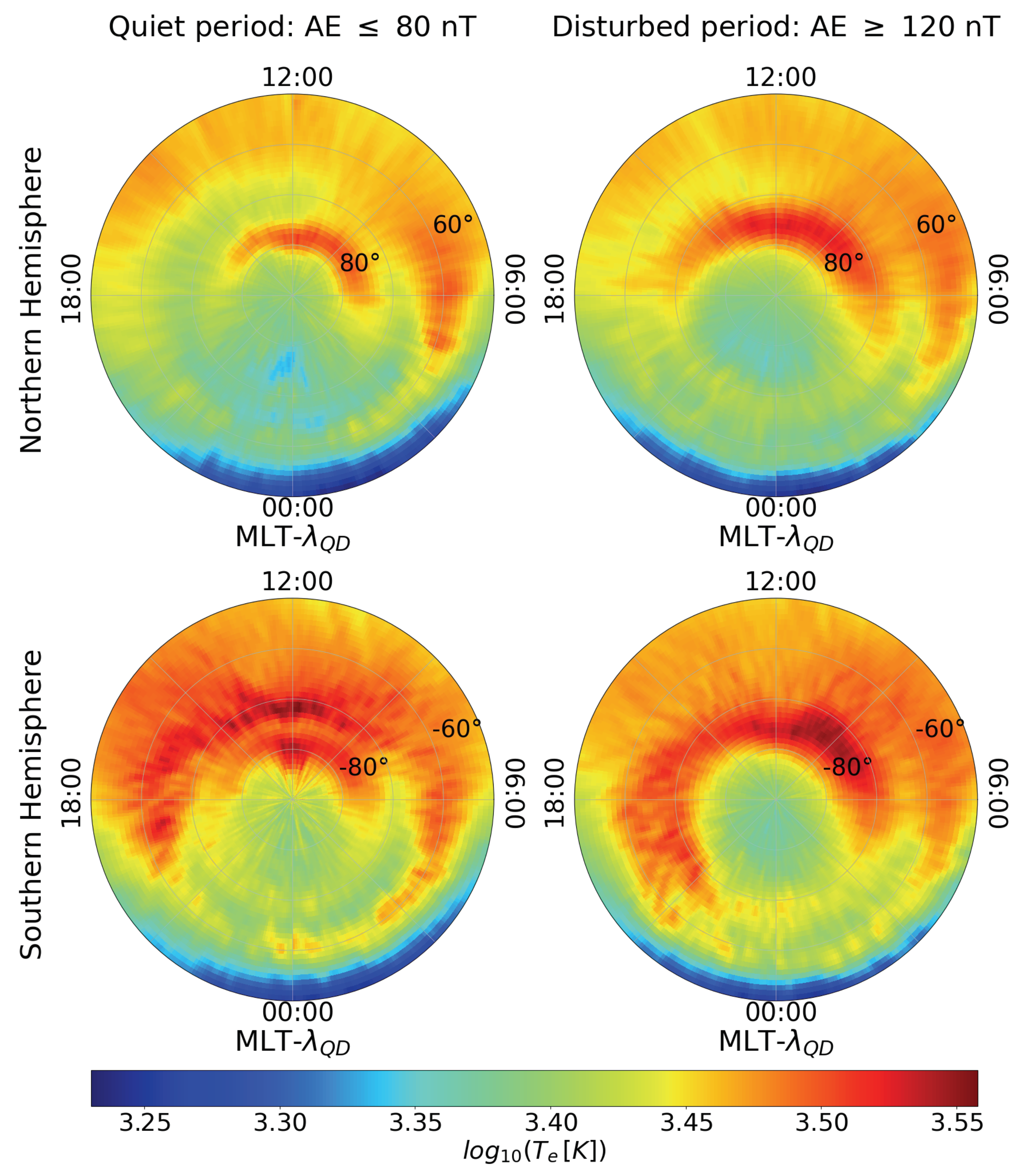
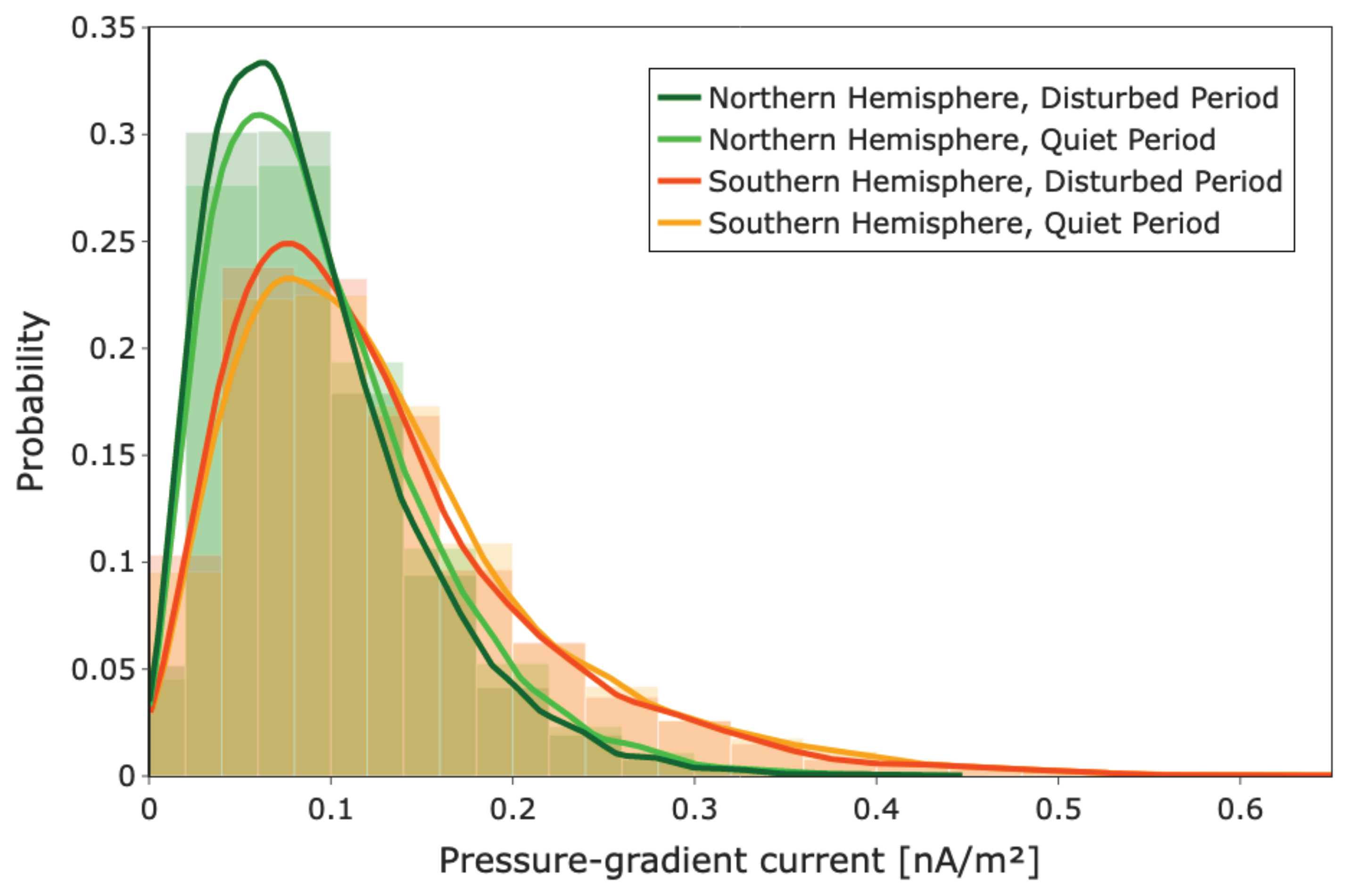
3.1. Variation of Pressure-Gradient Current with Geomagnetic Activity Level

The analysis of the current density spatial distribution due to pressure-gradient force at high latitude in the Northern and Southern hemispheres starts investigating the dependence on the geomagnetic activity level. Using the AE index we select two different levels of geomagnetic activity. Quiet periods correspond to values of $AE\le 80$ nT while disturbed ones to $AE\ge 120$ nT [26,27]. The two selected activity levels are chosen in order to clearly separate active and quiet periods according to the distribution function of AE index values, which is bimodal with a crossover around 100 nT. For this type of analysis we consider the whole dataset, that is, the electron density, electron temperature, and magnetic field recorded by Swarm A from 1 April 2014 to 28 February 2018.

Figure 1, Figure 2 and Figure 3 report a polar view of the large-scale spatial distribution of electron density ($N_e$), electron temperature ($T_e$), and plasma pressure (P) in the Northern and Southern hemispheres during quiet and disturbed periods, respectively. Data are mapped into grid binned at $1^{°}\times 1^{°}$ in QD latitude and MLT coordinates. The two selected geomagnetic activity levels correspond to different spatial distributions of the plasma parameters in the two hemispheres. Focusing on plasma pressure, we notice that its spatial distribution shows a clear dependence on magnetic latitude and magnetic local time (see Figure 3). It is characterized by a marked dayside/nigthside asymmetry, which mainly reflects the dayside/nigthside asymmetry of the electron density and temperature spatial distributions. Indeed, as reported in Figure 1, the electron density is generally almost twice in the dayside compared to the nightside due to the dependence of the electron density on the upper atmosphere ultraviolet ionization.

Moreover, a marked dayside/nigthside asymmetry also characterizes the spatial distribution of the electron temperature (see Figure 2) which is, even in this case, due to the increase of ultraviolet photoionization. However, the spatial distribution of the electron temperature also depends on the particle precipitation caused by magnetosphere-ionosphere coupling. Indeed, soft particle precipitation heats the F region ionosphere and is a likely source of the observed correlation of the anomalous density with elevated particle temperature. Thus, the magnetosphere-ionosphere coupling is responsible of the temperature enhancement both in the cusp region around noon [28], where particles of solar origin are directly injected into the ionosphere, and at auroral and sub-auroral latitudes where particles arrive directly from the geomagnetic tail regions and plasmasphere during disturbed periods (see Figure 2).

Not all the features of the electron density and electron temperature are recognizable in the plasma pressure spatial distribution. For example, the so-called main ionospheric trough (MIT), which corresponds to a prominent plasma depletion at subauroral regions during the night hours in a latitudinally limited band between ${60}^{°}$ and ${70}^{°}$ (see Figure 1), is not clearly recognizable in the pressure data. It is due to the fact that there is an electron temperature enhancement owing to the joint action of particle precipitation and decreased collisional cooling in correspondence with the main ionospheric trough [29,30]. In the nightside, at auroral and sub-auroral latitudes this process is dominant and becomes more and more important with the increase of the geomagnetic activity level (see Figure 2). Due to the anticorrelation between the electron density and electron temperature, the plasma pressure does not show a particular behaviour in this region. Conversely, Figure 3 reveals a plasma pressure depletion at low latitudes, between ${50}^{°}$ and ${65}^{°}$, in the nightside, between 21:00 and 06:00 MLT, whose position moves progressively to a lower latitude as the level of geomagnetic activity increases.

Another interesting feature of the plasma pressure is its marked increase in the cusp region around noon, which becomes more marked in the disturbed periods in both hemispheres. This increase is associated with the observed electron temperature and density enhancements.

Lastly, Figure 3 shows two other remarkable features, which mainly reflect $N_e$ spatial distribution features. There is an enhancement of plasma pressure from noon across the polar cap to the nightside during disturbed conditions in both hemispheres. This plasma pressure enhancement corresponds to the characteristic tongue of ionization (TOI) of $N_e$ [31,32], which is a large-scale feature of the F-region polar ionosphere. Furthermore, there is a plasma pressure increases around dusk in disturbed conditions reflecting the well-known storm-enhanced density (SED) plumes, which are prominent ionospheric electron density increases at the dayside mid and high latitudes [33].

Figure 4 reports the flow patterns of the plasma pressure-gradient current (black arrows) at high latitudes in the Northern and Southern hemispheres during the two different geomagnetic activity levels. Only for graphical reasons, the black arrows are mapped into grids binned at $2^{°}\times 4^{°}$ in QD latitude and MLT coordinates, where $4^{°}$ magnetic longitude corresponds to 16 min. Below the flow patterns of the reconstructed current there is the corresponding plasma pressure map, which permits us to better visualize the regions where the current develops. As expected, the current tends to flow around the plasma pressure enhancements and is stronger in region where the plasma pressure changes rapidly. Some well defined patterns can be recognized in the plasma pressure-gradient current regardless of geomagnetic activity level.

A vortex exists around the cleft region, whose position shifts equatorward as magnetic activity increases, following the natural shift of center of the precipitation region. Around the cleft region the current flows counter-clockwise in the Northern hemisphere and clockwise in the Southern one. This current flows in a direction which reduces the ambient geomagnetic field. At high latitude the magnetic field is nearly vertical and the horizontal pressure-gradient current produces a magnetic field which is, in first approximation, parallel to the main field but with opposite direction. Thus, the current produces a reduction of the magnetic field inside the plasma region around which the current flows. The existence of this current structure is indirectly confirmed by Park et al. [9] analysing the diamagnetic signatures of high-latitude ionospheric irregularities. In both hemispheres they found depletions in magnetic field strength of about 1 nT concentrated in the cusp region that they associated with the presence of local plasma irregularities with scale sizes below some hundred kilometers. Anyway, this region can be also characterized by large anomalies in the electron density correlated with intense small-scale magnetic fluctuations, which are associated with incident Alvén waves producing a local heating. This means that in this region an opposite scenario to that implicitly assumed may be possible: the observed pressure gradients may be also produced by magnetic disturbances [10].

At high latitudes (${\lambda }_{QD}>\left|{75}^{°}\right|$) the current flows counter-clockwise in the Northern hemisphere and in opposite direction in the Southern one. The spatial distribution of the current seems to identify, especially during disturbed periods, another region characterized by an enhancement of plasma density, which is due to the propagation of plasma from the cusp to the polar cap. This region, that is visible in both hemispheres, is known to be characterized by the presence of plasma instability and the formation of ionospheric irregularities known as polar cap patches, where the density is at least twice that of the background [34]. However, the reconstructed flow patterns of the pressure-gradient currents capture plasma pressure variations which are not necessary due to the presence of plasma density irregularities as for example polar cap patches and auroral blobs. At lower latitudes in the Northern and Southern hemispheres the flow pattern of the pressure-gradient current identifies another region where the ambient magnetic field can be reduced by this current. In first approximation, this region corresponds to the auroral zone from 15:00 MLT to 09:00 MLT, passing by 24:00 MLT. Thus, the pressure-gradient currents characterize also the auroral zone and equatorward of the auroral zone on the nigthside.

In general, the flow patterns of the pressure-gradient current are similar in both hemispheres and what one finds is their shift towards lower latitudes with the increase of the geomagnetic activity.

Figure 5 reports the distributions of the pressure-gradient current values for disturbed and quiet geomagnetic activity conditions for the Northern and Southern hemispheres. The comparison among the four distributions shows that the pressure-gradient current intensity is slightly higher in the Southern hemisphere than in the Northern one, while there is no great difference between quiet to disturbed periods. At high latitudes the mean values of these currents are quite low, around 1 order of magnitude less than the same diamagnetic currents observed at low latitudes [35]. Our findings are in agreement with previous studies. Analyzing two years of Swarm measurements Laundal et al. [11] estimated the small variations in the magnetic field strength due to pressure-gradient currents at polar latitudes by evaluating the magnetic field intensity variations anticorrelated with plasma density variations. As result of their statistical analysis, they showed that the polar caps, the auroral zone, and equatorward of the auroral zone on the nightside were the regions where the magnetic field variations were well explained by plasma pressure gradients. Their findings are slightly different from the results by Park et al. [9], where the highest occurrence rates between the magnetic field and the electron density variations are found in the auroral oval. In both papers the flow pattern of the pressure-gradient current is not calculated, nor its intensity. The existence of this current is invoked to justify the variations of magnetic field correlated with those of plasma density and climatological analyses of their correspondence are proposed. This means that, to make a comparison with our results, it is necessary to consider that the pressure-gradient currents flow around the plasma pressure enhancement regions, which are often characterized by the occurrence of ionospheric irregularities and are the regions identified in the previous papers. It is also important to notice that both Laundal et al. [11] and Park et al. [9] assume that the variations in plasma pressure are dominated by electron density, under the hypothesis of a local thermodynamic equilibrium, but looking at Figure 2 we notice that also the temperature plays a role in the plasma pressure, mainly in the auroral and sub-auroral latitudes.

To evaluate the pressure-gradient current we have used the magnetic field measurements recorded by Swarm A. It contains all the different contributes coming from its sources both internal (core and crust) and external (magnetospheric and ionospheric currents) to the Earth. In order to investigate the possible effect on the pressure-gradient current flow patterns of remote currents, in particular of those current systems that flow about 300 km below Swarm A and are expected to produce a smooth magnetic signature on the measured magnetic field [36], we evaluate the pressure-gradient current considering in this last case the magnetic field strength associated with internal sources. The internal part of the magnetic field is estimated using the CHAOS model [37]. Thus, the pressure-gradient current is evaluated and compared with that obtained using the ambient magnetic field. Figure 6 reports the percentage difference between the current evaluated in the two ways. This procedure should leave only the contribute of external sources to the pressure-gradient current. The effect on the pressure-gradient currents at Swarm altitude of the remote current systems is very low: it does not exceed $0.3\%$. However, it is not uniform, depending on the geographic location, magnetic local time, and geomagnetic activity level. Our findings show that the features of the reconstructed pressure-gradient currents at Swarm altitude depend only partially on geomagnetic field variations due to external disturbances, mainly they depend on the main field structures and on the features of pressure gradients.

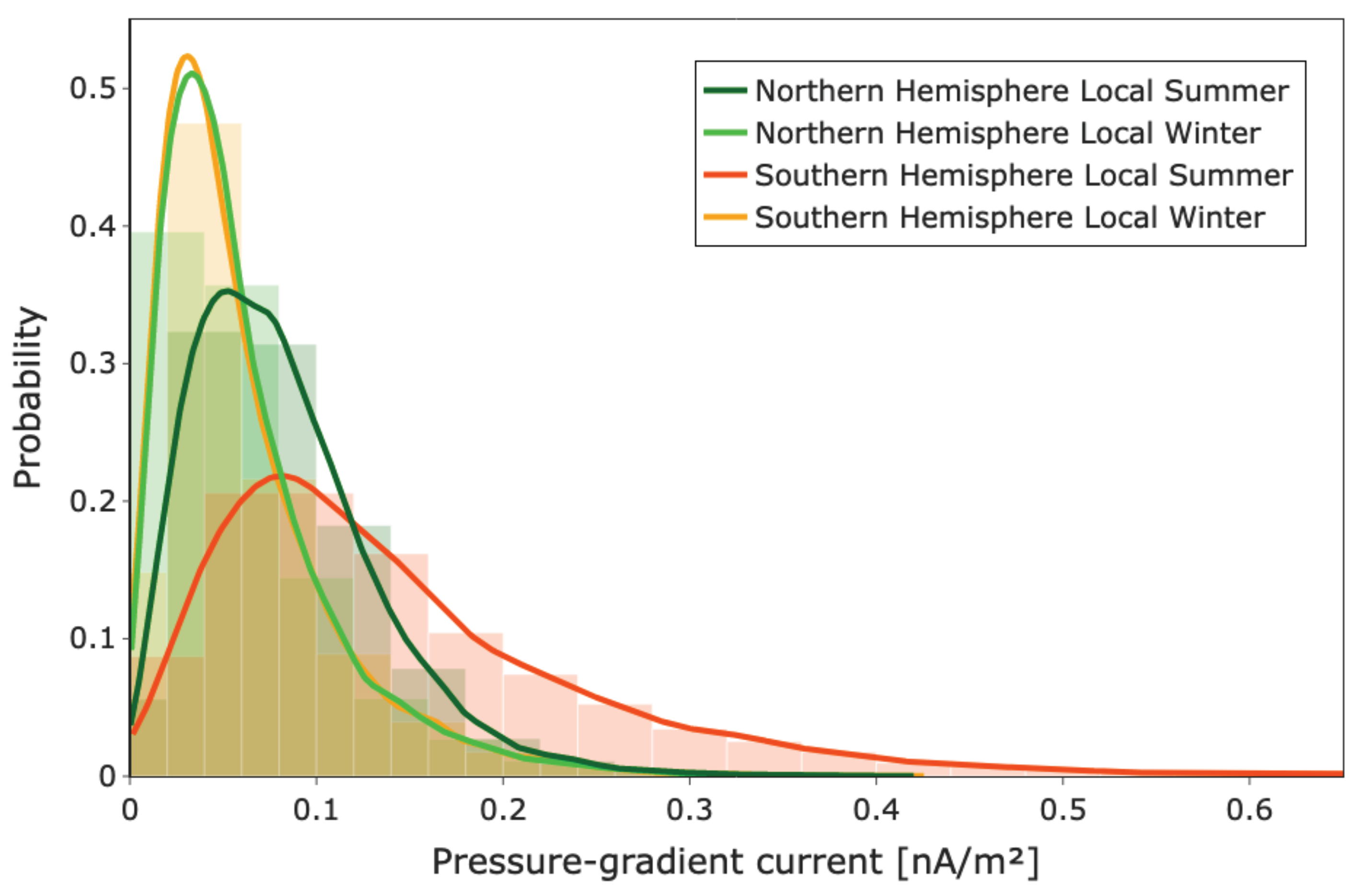
3.2. Variation of Pressure-Gradient Current with Season

In order to investigate the seasonal dependence of the pressure-gradient current, we consider the period between 5 May and 5 August of each year to identify the Northern local summer and the Southern local winter, and the period between 5 November and 5 February of each year to identify the Northern local winter and Southern local summer. Thus, by portioning the entire dataset according to summer and winter solstices, we can study the dependence of the pressure-gradient current on solar illumination.

Figure 7 reports the obtained plasma pressure distribution according to the selected seasons for both hemispheres, together with the resulting flow patterns of the pressure-gradient current. The current is described using black arrows whose lengths are proportional to the intensity. Differently from previous figures, we use different scales for the plasma pressure in the two seasons. Indeed, the plasma pressure is almost three times higher in summer than in winter. Looking at Figure 7 we notice that from winter to summer, there is an increase of plasma pressure in the dayside ionosphere at all MLTs, especially between the noon and the dusk at middle latitudes. Plasma pressure increases even in the post-nightside sector at low latitudes in the Southern hemisphere, and at high latitudes in the polar cap. Lastly, an increase is observable in the polar cusp during summer in both hemispheres.

The plasma pressure distributions reported in Figure 7 show that summer-winter asymmetry is more pronounced in the Southern hemisphere than in the Northern one. This is due to the different summer-winter asymmetry of $N_e$ spatial distribution between the two hemispheres, which is a combination of two different effects, the first produced by the solar radiation and the second by the F region annual anomaly [38,39]. Indeed, $N_e$ values are higher during summer than during winter, as a result of a larger solar radiation but, at the same time, they are higher during December solstice than during June one. Since in the Southern hemisphere the increase in $N_e$ values happens during summer season, it amplifies the difference with respect to local winter. Conversely, the F region annual anomaly has the effect of reducing the asymmetry between local seasons in the Northern hemisphere.

The dependence of the plasma pressure on the seasons also involves a dependence of the pressure-gradient current on the solar illumination. The flow patterns of the currents and their strengths change from winter to summer. The pressure-gradient currents are visible especially in summer where the structures, which have previously identified by studying the dependence on the geomagnetic activity levels, can be easily recognizable. Even in this case, we can observe three regions characterized by the presence of these currents, one around cleft region, another at high latitudes around the magnetic poles, and the third confined at auroral latitudes. These regions should identify the zones characterized by the occurrence of ionospheric irregularities.

As regards the current intensity in the two hemispheres during the two selected seasons, we report the distributions of the pressure-gradient current values in Figure 8. We notice that the current intensity is higher during summer than winter, when more plasma is produced by sunlight and plasma pressure gradients are greater. The current intensity is greater in the Southern hemisphere than Northern one.

3.3. Variation of Pressure-Gradient Current with Solar Activity

To evaluate the level of solar activity during the selected period of Swarm observations we use, as previously described, the daily solar flux at 10.7 cm (F10.7) and the Mg II core-to-wing ratio as proxies. The values of F10.7 and Mg II from 1 April 2014 to 31 December 2017 are reported in the lower panel of Figure 9. Here, the vertical dotted lines indicate the transition from one year to the next, the horizontal lines identify the yearly mean values, and the shaded parts cover the values between the yearly mean values ± one standard deviation year by year for each index. The analysed period corresponds to the decreasing phase of the solar cycle, and is characterized by a decrease in the F10.7 and Mg II yearly mean values.

For what concerns the pressure-gradient current intensity, the most remarkable features emerging from Figure 9 are a decrease in maximum and minimum values of the current intensity with the decrease of solar activity as well as a decrease of the intensity around the cusp. Moreover, regardless of the solar activity level, the pressure-gradient current is substantially more intense in the Southern hemisphere than in the Northern one at almost all magnetic latitudes and MLTs. In the Southern hemisphere, besides the three main regions already identified, another region of enhanced current is visible. It is at a latitude between ${70}^{°}$ and ${80}^{°}$ in the nightside. This structure is well visible in 2014 and 2015 when the solar activity is higher.

4. Discussion and Conclusions

The aim of the present research was to examine the flow patterns of the pressure-gradient currents and their strengths at high-latitude ionospheric topside F2 region in both hemispheres, and investigate their dependence on magnetic local time, geomagnetic activity, season and solar forcing drivers. All this has been achieved thanks to the geomagnetic field, electron density and electron temperature variations observed by Swarm A satellite from 2014 to 2018. The flow patterns of the pressure-gradient currents have been estimated under the hypothesis that it is possible to ignore the effects of neutral collisions and consider the electron and ion temperature equal. Our study is the first to show polar flow patterns of the pressure-gradient currents and their strengths at Swarm altitude. From the observations the following conclusions can be drawn:

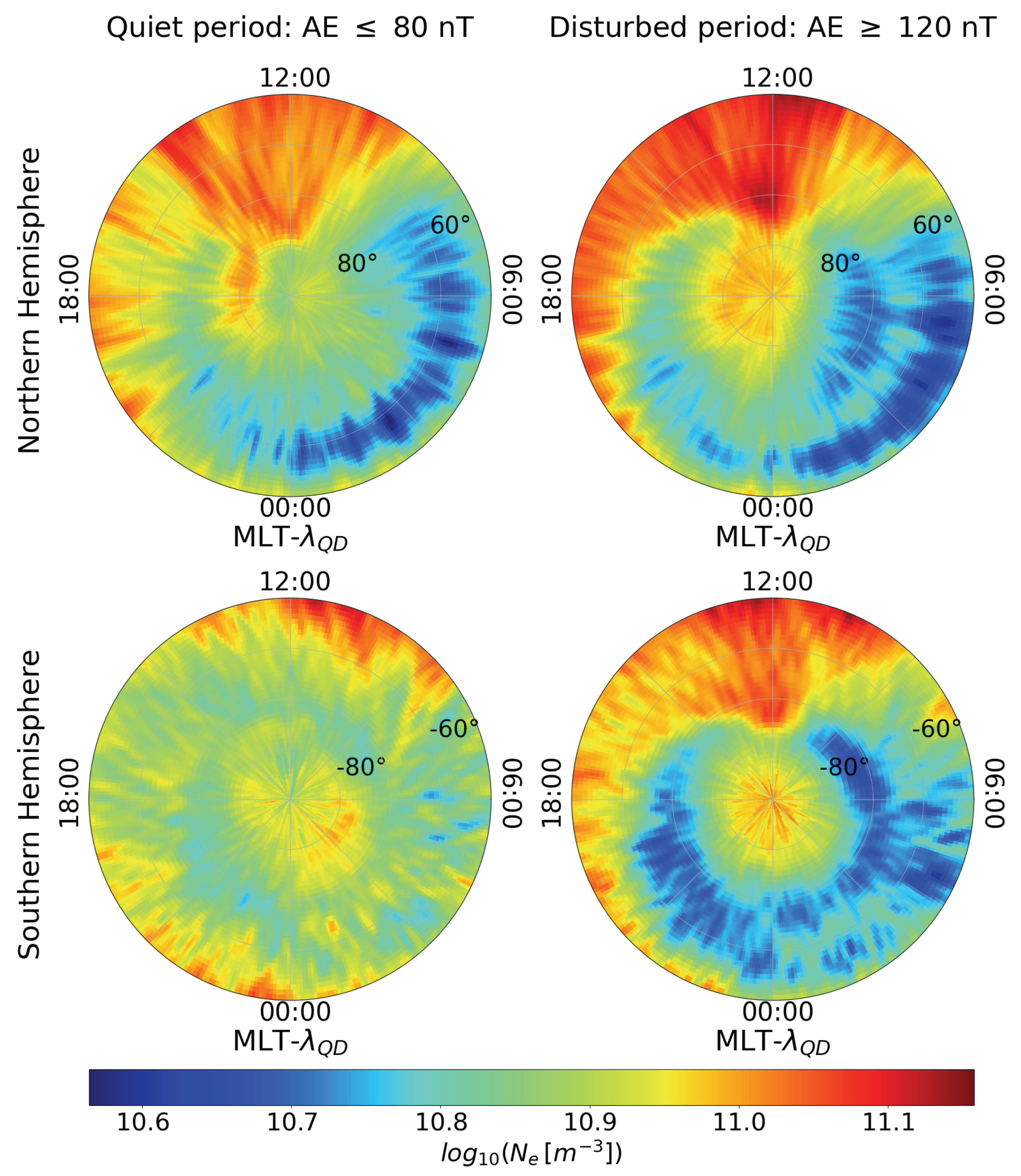
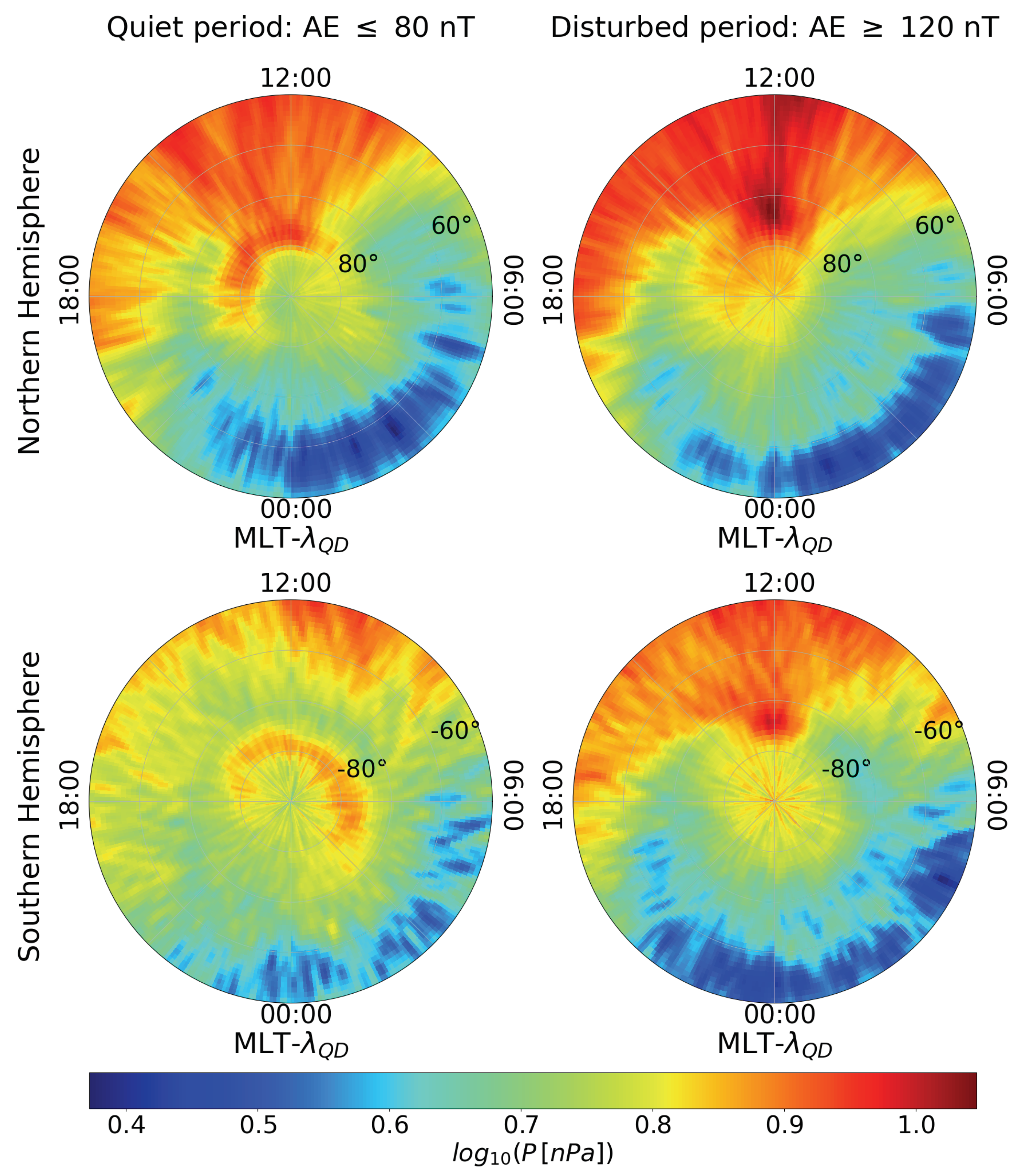
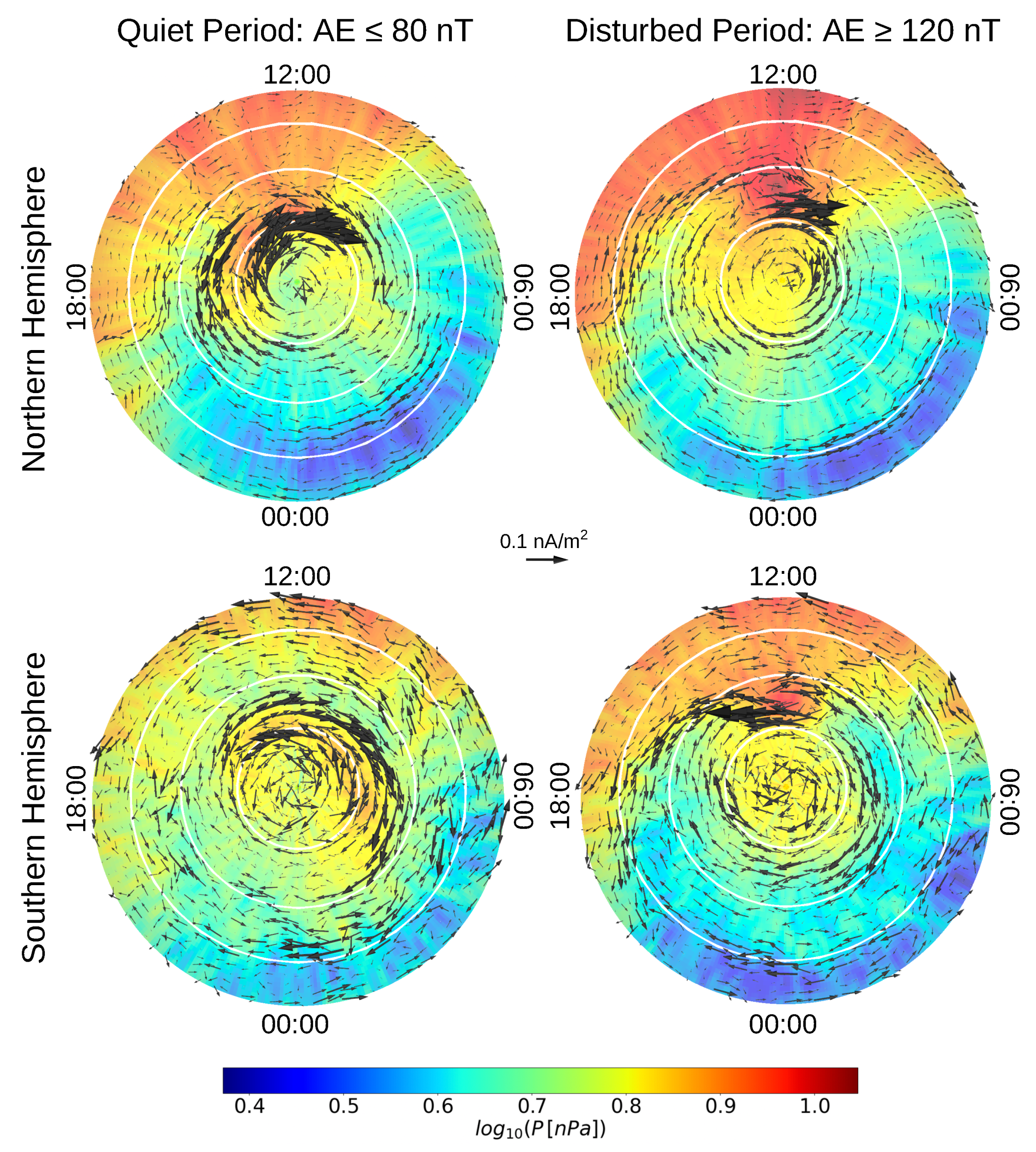
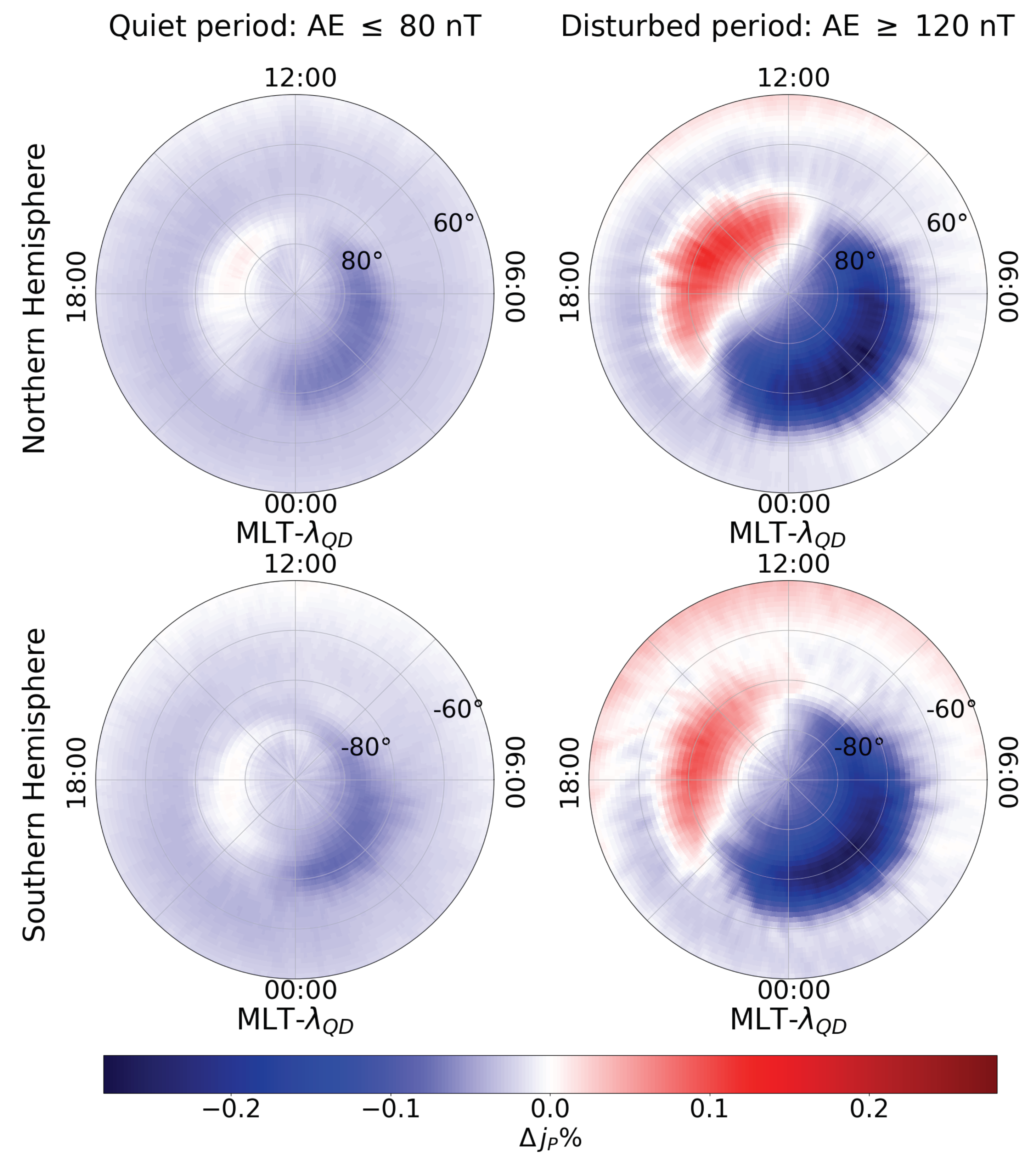
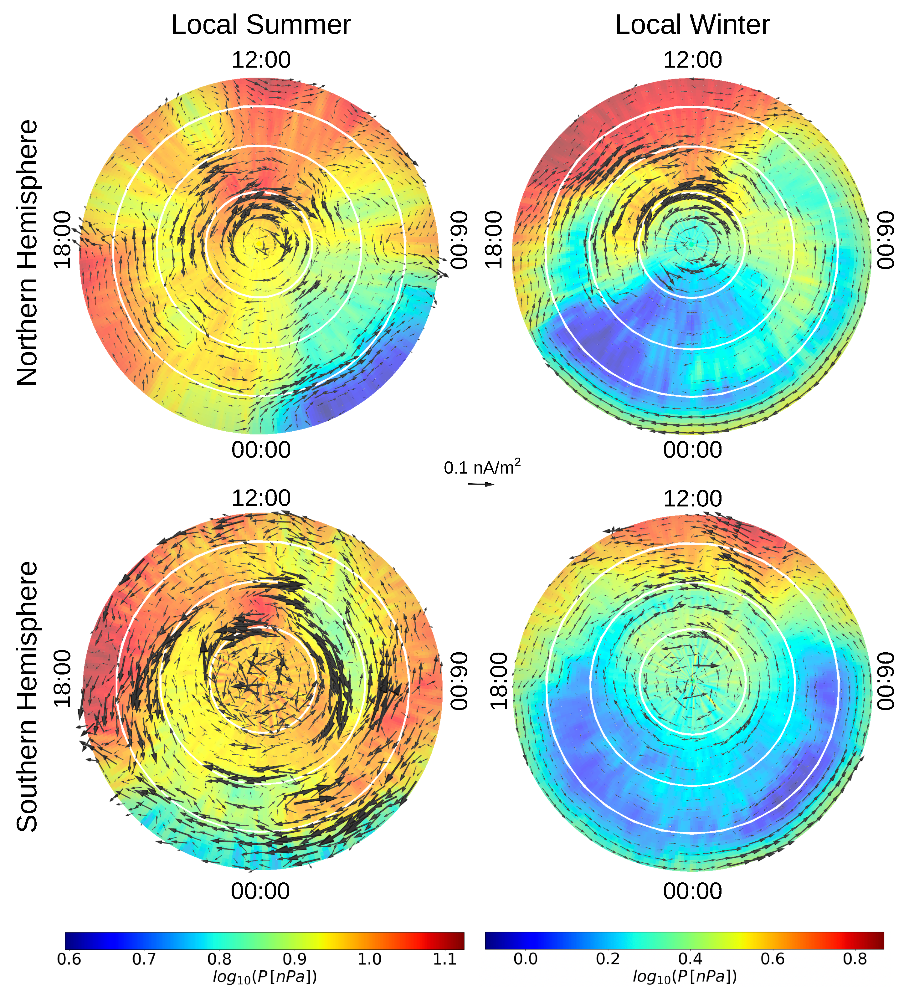
• During geomagnetically disturbed periods ($AE\ge 120$ nT) the plasma pressure gradients are particularly large around cleft region, where the electron density is changing rapidly. The pressure-gradient current flows around this plasma pressure enhancement region in both hemispheres. The existence of this flow pattern agrees with an increased probability of finding magnetic field variations correlated with plasma density ones around cleft region [9]. Anyway, we remark that additional contributions to the observed magnetic field variations and plasma pressure gradients can be due to incident Alfvén wave [10];
• Regardless of the level of geomagnetic activity, at high latitudes (${\lambda }_{QD}>\left|{75}^{°}\right|$) the flow patterns of the pressure-gradient current identify another region characterized by large plasma pressure gradients, the polar cap. This region, that is observable in both hemispheres, is known to be characterized by the presence of plasma instabilities and the formation of ionospheric irregularities [34]. Additionally, in this region previous studies [11] found a high occurrence rate of magnetic field variations well explained by plasma density variations;
• At lower latitudes in both hemispheres the flow patterns of the pressure-gradient current identify another region where the plasma pressure is changing. In first approximation, it corresponds to the auroral oval and equatorward of the auroral oval on the nigthside. These flow patterns move to lower geomagnetic latitude with increasing geomagnetic activity;
• The pressure-gradient current mean intensity is quite low, around 1 order of magnitude less than the same current observed at low latitudes. In addition, the mean value found in our analysis is lower than that obtained by Laundal et al. [11] at high latitude. The reasons are probably due to the different method used to estimate the currents and to the different size of the window used to evaluate the pressure gradients. We use a window larger than the one used by Laundal et al. [11] and for this reason our pressure gradients are sharper and the pressure-gradient current intensities are smaller.
• Pressure-gradient current shows a clear dependence on solar illumination, and its intensity is influenced by F region annual anomaly. This is probably the reason why the asymmetry summer/winter is more marked in the Southern hemisphere than in the Northern one. Using the diamagnetic effect, Park et al. [9] and Laundal et al. [11] investigated the dependence on season of the ionospheric irregularity occurrences at high latitude. In some ways, our findings are in agreement with those reported by Laundal et al. [11], who found higher occurrence rates of magnetic field variations well explained by plasma pressure in summer than winter. However, the region characterized by a higher probability to find a correspondence between magnetic field and electron density variations is mainly confined in the polar cap in Laundal et al. [11], while the geographic location of our currents is wider. Nevertheless, a more precise comparison is not possible since there is not a distinction between the two hemispheres in Laundal et al. [11]. Conversely, the findings of our study do not seem to support the previous research by Park et al. [9], who reported higher occurrence rates of plasma density irregularities in winter than summer. This is probably due to a different data selection, Park et al. [9] studied the seasonal dependence considering measurements relative to geomagnetically active periods ($AE\ge 200$ nT). We study the seasonal dependence regardless of geomagnetic activity level and in our selection the percentage of data, that satisfies the AE threshold fixed by Park et al. [9], is approximately of $28\%$;
• Regardless of geomagnetic and solar activity, the pressure-gradient current intensity is always slightly greater in the Southern hemisphere than in the Northern one;
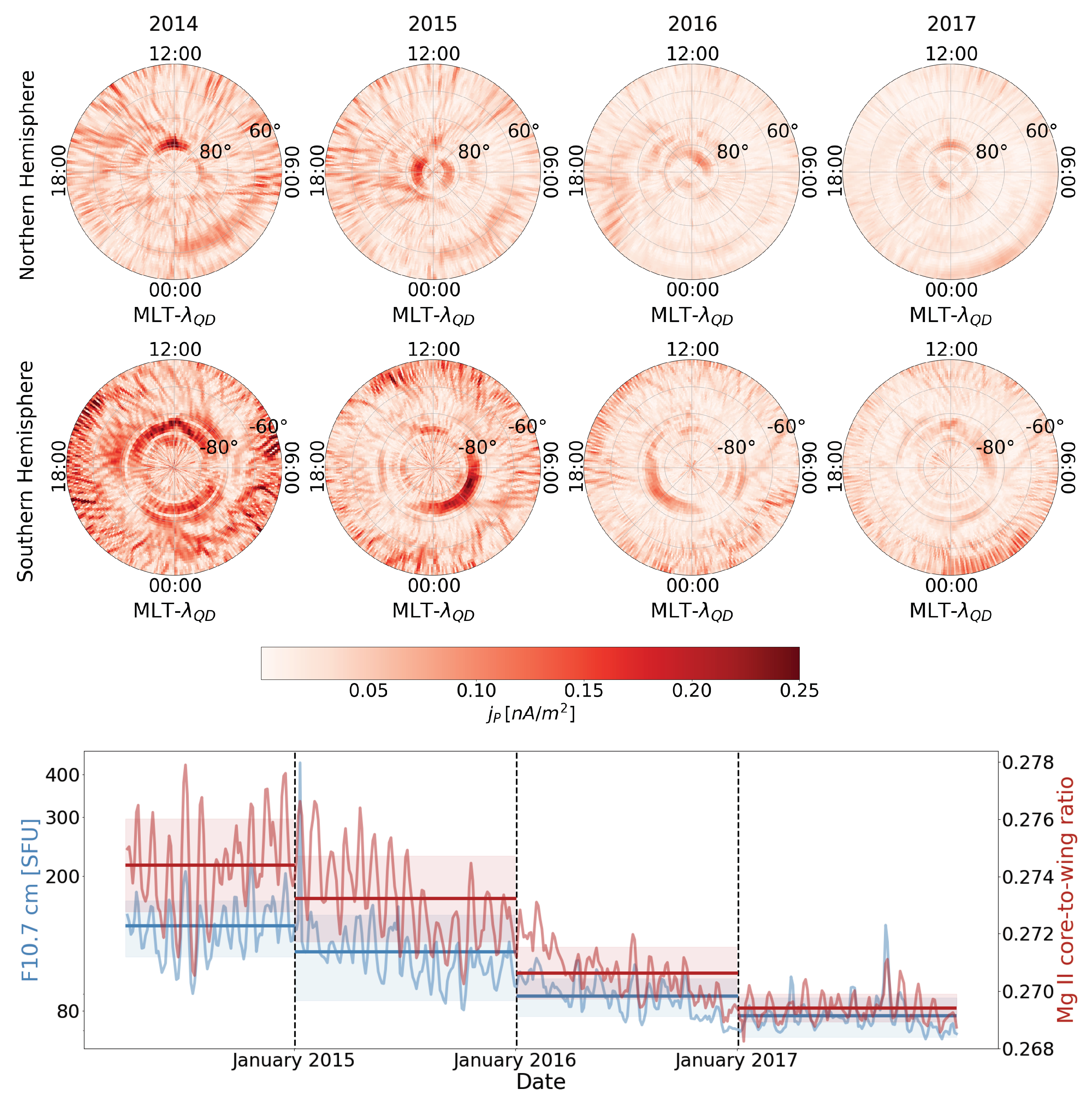
• The pressure-gradient current intensity decreases with the solar activity level.

The findings of this study confirm that the strength of the pressure-gradient currents is weak in the high-latitude ionospheric topside F2 region, at Swarm A altitude (≃460 km), but these currents appear preferentially at the same geographic locations regardless of geomagnetic activity, season and solar activity. This means that the magnetic field variations associated with these flow patterns can induce disturbances on the ionospheric magnetic field measurements and cause artifacts in main field models.

References

1. Cravens, T.; Dessler, A.; Houghton, J.; Rycroft, M. Physics of Solar System Plasmas; Cambridge University Press: Cambridge, UK, 1997. [Google Scholar]
2. Ganushkina, N.; Liemohn, M.; Dubyagin, S. Current systems in the Earth’s magnetosphere. Rev. Geophys. 2018, 56, 309–332. [Google Scholar] [CrossRef]
3. Lühr, H.; Rother, M.; Maus, S.; Mai, W.; Cooke, D. The diamagnetic effect of the equatorial Appleton anomaly: Its characteristics and impact on geomagnetic field modeling. Geophys. Res. Lett. 2003, 30. [Google Scholar] [CrossRef] [Green Version]
4. Reigber, C.; Schwintzer, P.; Neumayer, K.; Barthelmes, F.; König, R.; Förste, C.; Balmino, G.; Biancale, R.; Lemoine, J.; Loyer, S.; et al. The CHAMP-only Earth gravity field model EIGEN-2. Adv. Space Res. 2003, 31, 1883–1888. [Google Scholar] [CrossRef]
5. Lühr, H.; Maus, S. Solar cycle dependence of quiet-time magnetospheric currents and a model of their near-Earth magnetic fields. Earth Planets Space 2010, 62, 843–848. [Google Scholar] [CrossRef] [Green Version]
6. Alken, P.; Maus, S.; Richmond, A.; Maute, A. The ionospheric gravity and diamagnetic current systems. J. Geophys. Res. Space Phys. 2011, 116, A12316. [Google Scholar] [CrossRef]
7. Richmond, A.; Ridley, E.; Roble, R. A thermosphere/ionosphere general circulation model with coupled electrodynamics. Geophys. Res. Lett. 1992, 19, 601–604. [Google Scholar] [CrossRef]
8. Alken, P. Observations and modeling of the ionospheric gravity and diamagnetic current systems from CHAMP and Swarm measurements. J. Geophys. Res. Space Phys. 2016, 121, 589–601. [Google Scholar] [CrossRef] [Green Version]
9. Park, J.; Ehrlich, R.; Lühr, H.; Ritter, P. Plasma irregularities in the high-latitude ionospheric F region and their diamagnetic signatures as observed by CHAMP. J. Geophys. Res. Space Phys. 2012, 117, A10322. [Google Scholar] [CrossRef] [Green Version]
10. Lotko, W.; Zhang, B. Alfvénic heating in the cusp ionosphere-thermosphere. J. Geophys. Res. Space Phys. 2018, 123, 10–368. [Google Scholar] [CrossRef]
11. Laundal, K.; Hatch, S.; Moretto, T. Magnetic effects of plasma pressure gradients in the upper F region. Geophys. Res. Lett. 2019, 46, 2355–2363. [Google Scholar] [CrossRef] [Green Version]
12. Friis-Christensen, E.; Lühr, H.; Hulot, G. Swarm: A constellation to study the Earth’s magnetic field. Earth Planets Space 2006, 58, 351–358. [Google Scholar] [CrossRef] [Green Version]
13. Knudsen, D.; Burchill, J.; Buchert, S.; Eriksson, A.; Gill, R.; Wahlund, J.; Åhlén, L.; Smith, M.; Moffat, B. Thermal ion imagers and Langmuir probes in the Swarm electric field instruments. J. Geophys. Res. Space Phys. 2017, 122, 2655–2673. [Google Scholar] [CrossRef]
14. Lomidze, L.; Knudsen, D.; Burchill, J.; Kouznetsov, A.; Buchert, S. Calibration and validation of Swarm plasma densities and electron temperatures using ground-based radars and satellite radio occultation measurements. Radio Sci. 2018, 53, 15–36. [Google Scholar] [CrossRef] [Green Version]
15. Richmond, A.D. Ionospheric electrodynamics using magnetic apex coordinates. J. Geomagn. Geoelectr. 1995, 47, 191–212. [Google Scholar] [CrossRef]
16. Emmert, J.; Richmond, A.; Drob, D. A computationally compact representation of Magnetic-Apex and Quasi-Dipole coordinates with smooth base vectors. J. Geophys. Res. Space Phys. 2010, 115, A08322. [Google Scholar] [CrossRef]
17. Laundal, K.; Richmond, A. Magnetic coordinate systems. Space Sci. Rev. 2017, 206, 27–59. [Google Scholar] [CrossRef] [Green Version]
18. Baker, K.; Wing, S. A new magnetic coordinate system for conjugate studies at high latitudes. J. Geophys. Res. Space Phys. 1989, 94, 9139–9143. [Google Scholar] [CrossRef]
19. Peeters, P.; Simon, P.; White, O.; De Toma, G.; Rottman, G.; Woods, T.; Knapp, B. Mg II Core-to-Wing Solar Index from High Resolution GOME Data. 1997. Available online: https://earth.esa.int/workshops/ers97/papers/peeters3/index-2.html (accessed on 3 March 2022).
20. Snow, M.; Machol, J.; Viereck, R.; Woods, T.; Weber, M.; Woodraska, D.; Elliott, J. A revised magnesium II core-to-wing ratio from SORCE SOLSTICE. Earth Space Sci. 2019, 6, 2106–2114. [Google Scholar] [CrossRef]
21. Foukal, P. Extension of the F10.7 index to 1905 using Mt. Wilson Ca K spectroheliograms. Geophys. Res. Lett. 1998, 25, 2909–2912. [Google Scholar] [CrossRef]
22. Tapping, K. The 10.7 cm solar radio flux (F10.7). Space Weather 2013, 11, 394–406. [Google Scholar] [CrossRef]
23. Richmond, A.; Maute, A. Ionospheric electrodynamics modeling. In Modeling the Ionosphere-Thermosphere System; American Geophysical Union: Washington, DC, USA, 2014; pp. 57–71. [Google Scholar]
24. Kamide, Y.; Chian, A. Handbook of the Solar-Terrestrial Environment; Springer: Berlin/Heidelberg, Germany, 2007. [Google Scholar]
25. Quarteroni, A.; Sacco, R.; Saleri, F. Numerical Mathematics; Springer-Verlag New York, Inc.: New York, NY, USA, 2010; Volume 58. [Google Scholar]
26. Consolini, G. Self-organized criticality: A new paradigm for the magnetotail dynamics. Fractals 2002, 10, 275–283. [Google Scholar] [CrossRef]
27. Alberti, T.; Giannattasio, F.; De Michelis, P.; Consolini, G. Linear versus nonlinear methods for detecting magnetospheric and ionospheric current systems patterns. Earth Space Sci. 2020, 7, e2019EA000559. [Google Scholar] [CrossRef] [Green Version]
28. Milan, S.; Provan, G.; Hubert, B. Magnetic flux transport in the Dungey cycle: A survey of dayside and nightside reconnection rates. J. Geophys. Res. Space Phys. 2007, 112. [Google Scholar] [CrossRef]
29. Wang, W.; Burns, A.; Killeen, T. A numerical study of the response of ionospheric electron temperature to geomagnetic activity. J. Geophys. Res. Space Phys. 2006, 111. [Google Scholar] [CrossRef] [Green Version]
30. Prölss, G. Subauroral electron temperature enhancement in the nighttime ionosphere. Ann. Geophys. 2006, 24, 1871–1885. [Google Scholar] [CrossRef] [Green Version]
31. Knudsen, W. Magnetospheric convection and the high-latitude F 2 ionosphere. J. Geophys. Res. 1974, 79, 1046–1055. [Google Scholar] [CrossRef] [Green Version]
32. Foster, J.; Coster, A.; Erickson, P.; Holt, J.; Lind, F.; Rideout, W.; McCready, M.; Van Eyken, A.; Barnes, R.; Greenwald, R.; et al. Multiradar observations of the polar tongue of ionization. J. Geophys. Res. Space Phys. 2005, 110. [Google Scholar] [CrossRef] [Green Version]
33. Foster, J. Storm time plasma transport at middle and high latitudes. J. Geophys. Res. Space Phys. 1993, 98, 1675–1689. [Google Scholar] [CrossRef]
34. Spicher, A.; Clausen, L.; Miloch, W.; Lofstad, V.; Jin, Y.; Moen, J. Interhemispheric study of polar cap patch occurrence based on Swarm in situ data. J. Geophys. Res. Space Phys. 2017, 122, 3837–3851. [Google Scholar] [CrossRef]
35. Alken, P.; Maute, A.; Richmond, A. The F-Region Gravity and Pressure Gradient Current Systems: A Review. Space Sci. Rev. 2017, 206, 451–469. [Google Scholar] [CrossRef]
36. Olsen, N. A new tool for determining ionospheric currents from magnetic satellite data. Geophys. Res. Lett. 1996, 23, 3635–3638. [Google Scholar] [CrossRef]
37. Finlay, C.; Olsen, N.; Tøffner-Clausen, L. DTU candidate field models for IGRF-12 and the CHAOS-5 geomagnetic field model. Earth Planets Space 2015, 67, 114. [Google Scholar] [CrossRef] [Green Version]
38. Torr, D.; Torr, M.; Richards, P. Causes of the F region winter anomaly. Geophys. Res. Lett. 1980, 7, 301–304. [Google Scholar] [CrossRef]
39. Rishbeth, H.; Müller-Wodarg, I. Why is there more ionosphere in January than in July? The annual asymmetry in the F2-layer. Ann. Geophys. 2006, 24, 3293–3311. [Google Scholar] [CrossRef] [Green Version]
Figure 1. Polar view of the average spatial distribution of electron density ( N e ) for quiet (left column) and disturbed (right column) geomagnetic activity conditions, for the Northern and Southern hemispheres, in QD-latitude ( λ Q D > 50 ° and λ Q D < 50 ° for the Northern and Southern hemisphere, respectively) and MLT reference system. Maps are obtained using data recorded by Swarm A from 1 April 2014 to 28 February 2018. The concentric dashed circles represent contours of magnetic latitude separated by 10 ° .
Remotesensing 14 01428 g001
Figure 2. Polar view of the average spatial distribution of electron temperature ( T e ) for quiet (left column) and disturbed (right column) geomagnetic activity conditions, for the Northern and Southern hemispheres, in QD-latitude ( λ Q D > 50 ° and λ Q D < 50 ° for the Northern and Southern hemisphere, respectively) and MLT reference system. Maps are obtained using data recorded by Swarm A from 1 April 2014 to 28 February 2018. The concentric dashed circles represent contours of magnetic latitude separated by 10 ° .
Remotesensing 14 01428 g002
Figure 3. Polar view of the average spatial distribution of plasma pressure for quiet (left column) and disturbed (right column) geomagnetic activity conditions, for the Northern and Southern hemispheres, in QD-latitude ( λ Q D > 50 ° and λ Q D < 50 ° for the Northern and Southern hemisphere, respectively) and MLT reference system. Maps are obtained using data recorded by Swarm A from 1 April 2014 to 28 February 2018. The concentric dashed circles represent contours of magnetic latitude separated by 10 ° .
Remotesensing 14 01428 g003
Figure 4. Flow patterns of pressure-gradient current (black arrows) superimposed on the plasma pressure spatial distribution for quiet (left column) and disturbed (right column) geomagnetic activity conditions, for the Northern and Southern hemispheres, in QD-latitude ( λ Q D > | 50 ° | ) and MLT reference system. Maps are obtained using data recorded by Swarm A from 1 April 2014 to 28 February 2018. For graphical reasons, the current’s vector field is mapped into grids binned at 2 ° × 4 ° , where 4 ° magnetic longitude corresponds to 16 min. The concentric white circles are plotted in 10 ° intervals, corresponding to QD-latitudes of | 80 ° | , | 70 ° | and | 60 ° | starting from the centre, respectively.
Remotesensing 14 01428 g004
Figure 5. Distributions of the pressure-gradient current values for disturbed and quiet geomagnetic activity conditions for the Northern and Southern hemispheres. Solid line represents the continuous probability density curve and it is plotted above the more transparent relative histogram.
Remotesensing 14 01428 g005
Figure 6. Difference in percentage between the pressure-gradient current evaluated using the magnetic field measured by Swarm A and that evaluated using the magnetic field of internal origin, in the case of quiet (left column) and disturbed (right column) geomagnetic activity conditions, for the Northern and Southern hemispheres, in QD-latitude ( λ Q D > 50 ° and λ Q D < 50 ° for the Northern and Southern hemisphere, respectively) and MLT reference system.
Remotesensing 14 01428 g006
Figure 7. Flow patterns of pressure-gradient current (black arrows) superimposed on the plasma pressure distribution during summer (left column) and winter (right column) periods, in the Northern and Southern hemispheres. Maps are in QD-latitude ( λ Q D > | 50 ° | ) and MLT reference system. The binning window is 1 ° λ Q D × 4 MLT for the pressure map, while for the current’s vector field the window is 2 ° λ Q D × 16 MLT for graphical reasons. The concentric white circles are plotted in 10 ° interval, corresponding to QD-latitudes of | 80 ° | , | 70 ° | and | 60 ° | starting from the centre.
Remotesensing 14 01428 g007
Figure 8. Distributions of the pressure-gradient current values for local summer and local winter conditions in the Northern and Southern hemispheres. Solid line represents the continuous probability density curve and is plotted above the more transparent relative histogram.
Remotesensing 14 01428 g008
Figure 9. From top to bottom: Polar view of the average spatial distribution of the pressure-gradient current intensities, year by year, for the Northern and Southern hemisphere, respectively; F10.7 (blue) and the Mg II (red) indices during the 4 years of Swarm observations. The vertical dotted lines indicate the transition from one year to the next, the horizontal lines identify the yearly mean values, while the shaded parts cover the values between the yearly mean values ± one standard deviation year by year for each index.
Remotesensing 14 01428 g009
Publisher’s Note: MDPI stays neutral with regard to jurisdictional claims in published maps and institutional affiliations.