
Spatial–Temporal Land Loss Modeling and Simulation in a Vulnerable Coast: A Case Study in Coastal Louisiana


 ,
,  ,
,  ,
, 
 and
and
Abstract
:1. Introduction
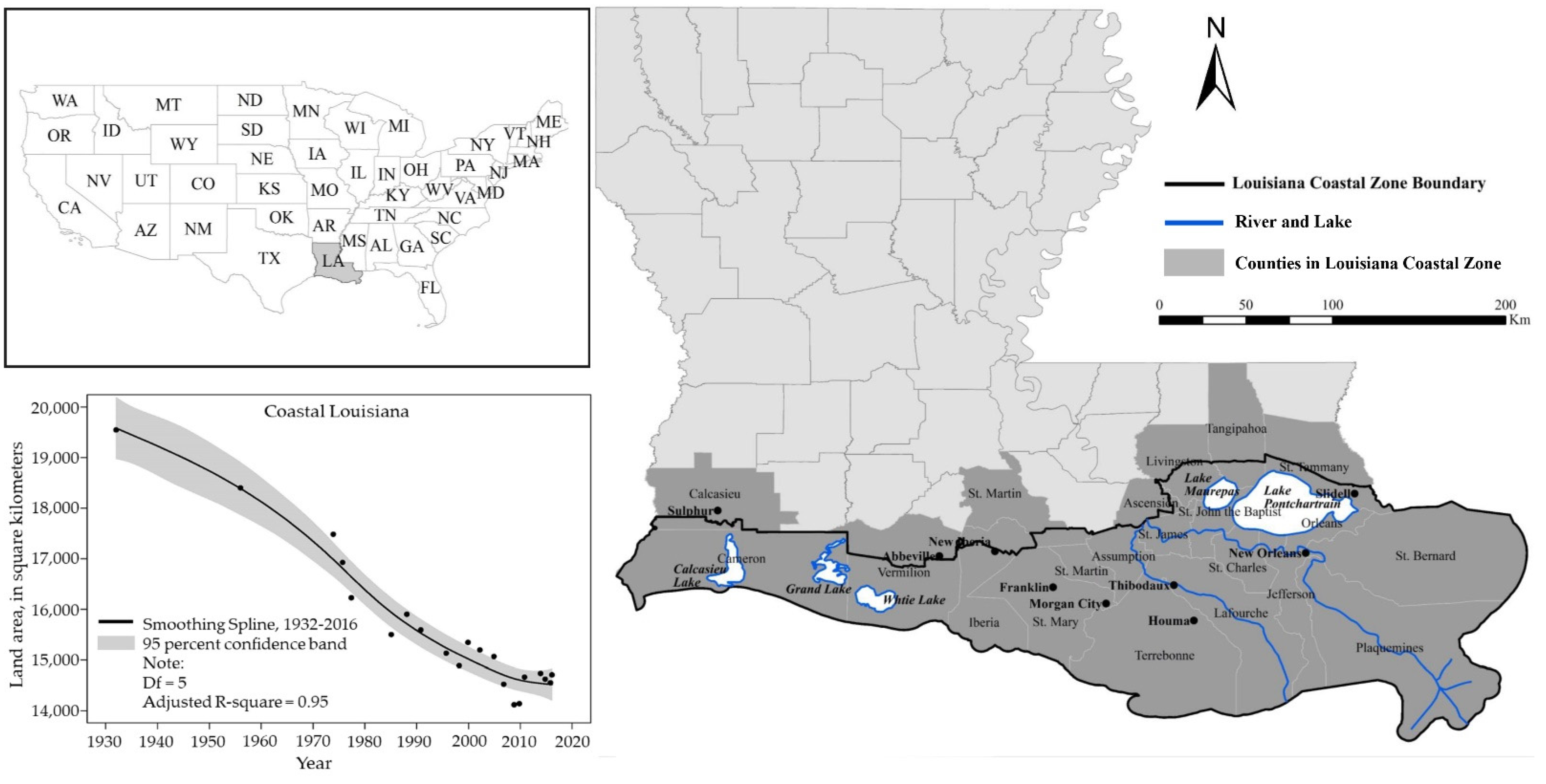
2. Study Area
Related Research
3. Materials
3.1. Land Use and Land Cover Data
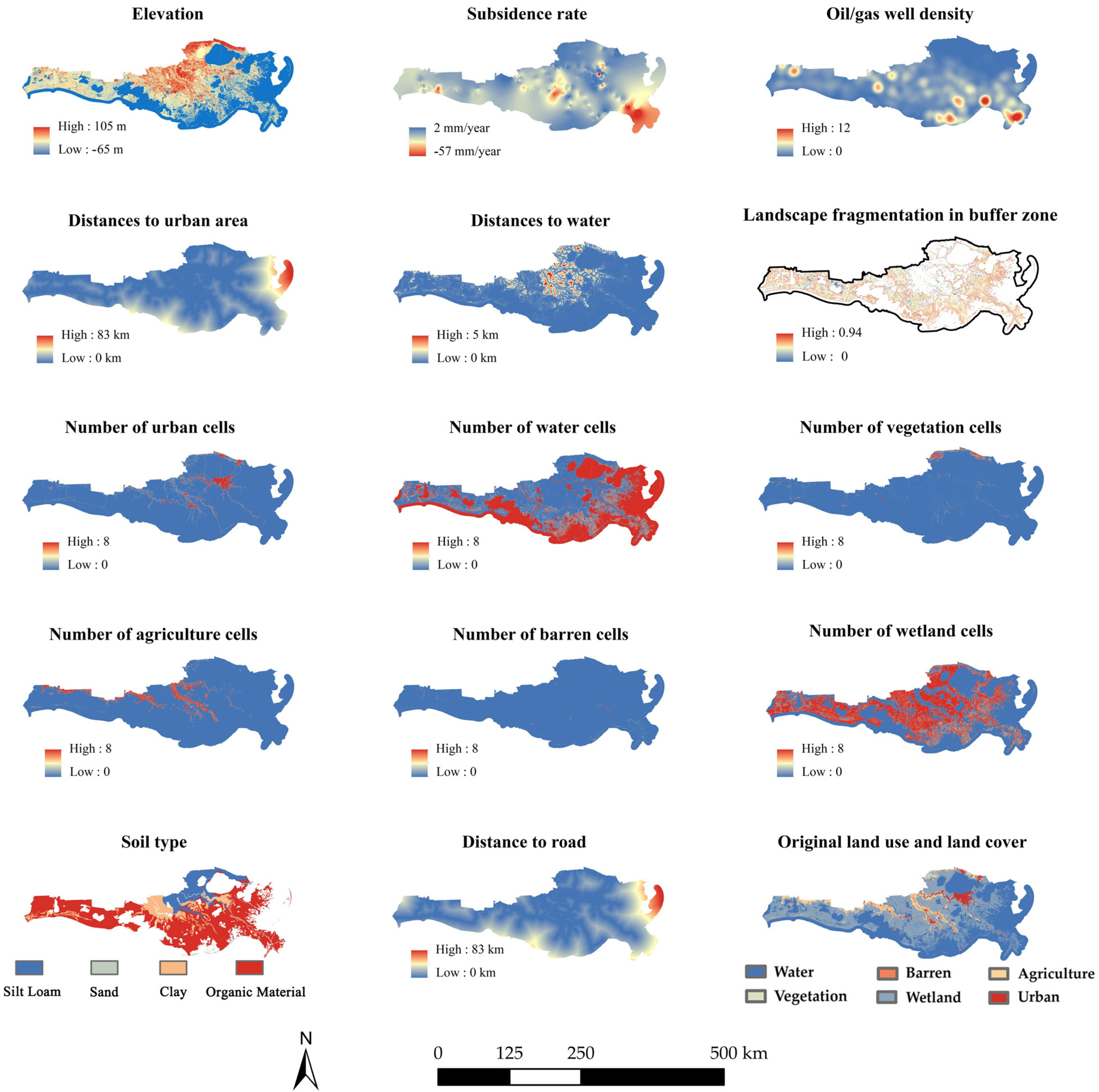
3.2. Human–Environmental Variables
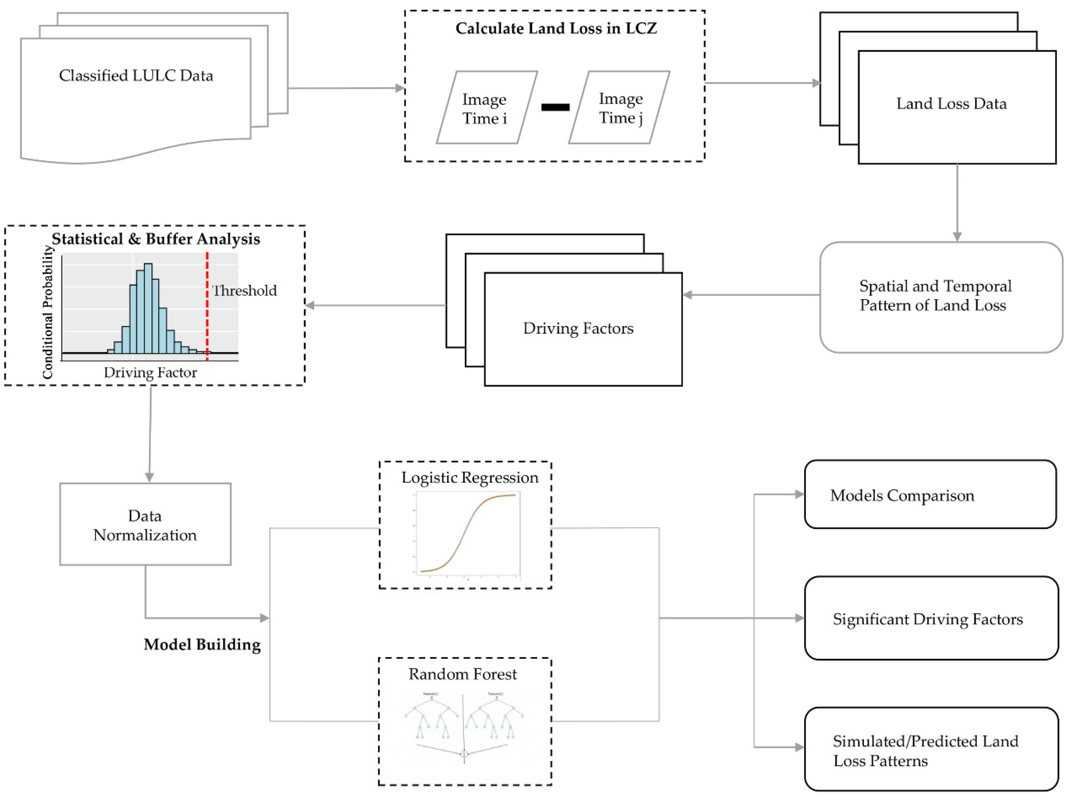
4. Methodology
4.1. Statistical Analysis
4.2. Machine Learning
4.3. Accuracy Analysis
5. Results
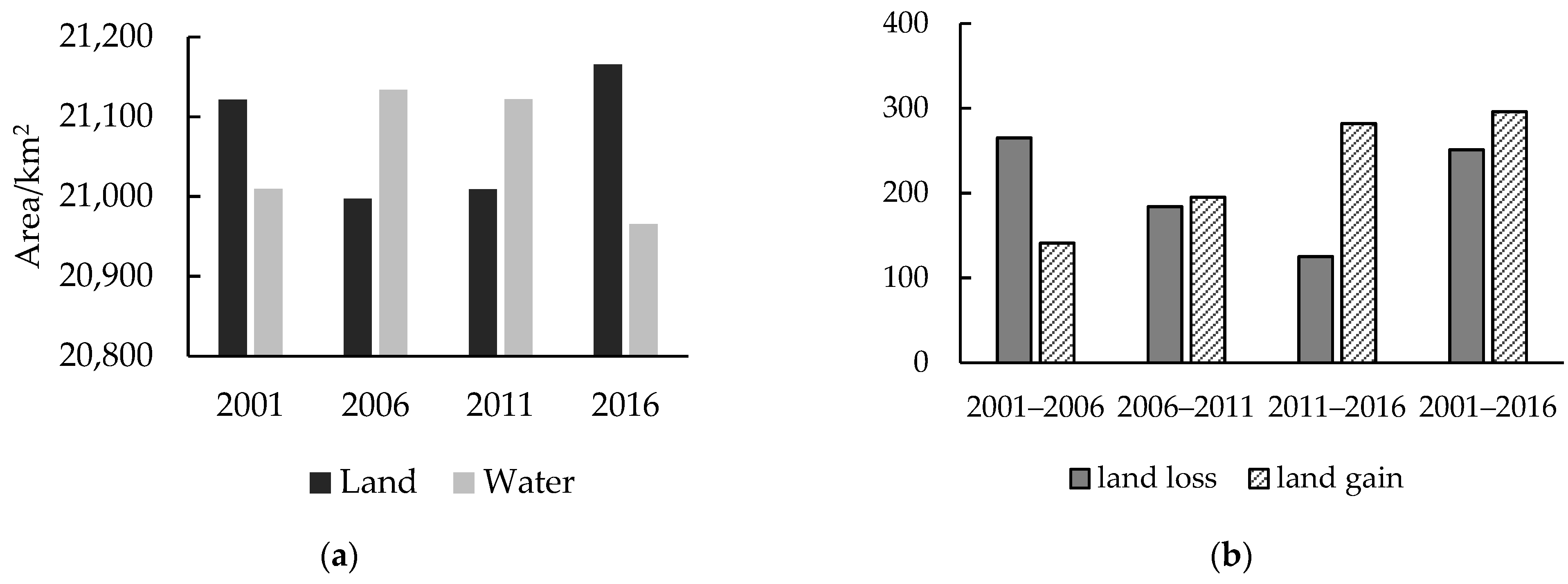
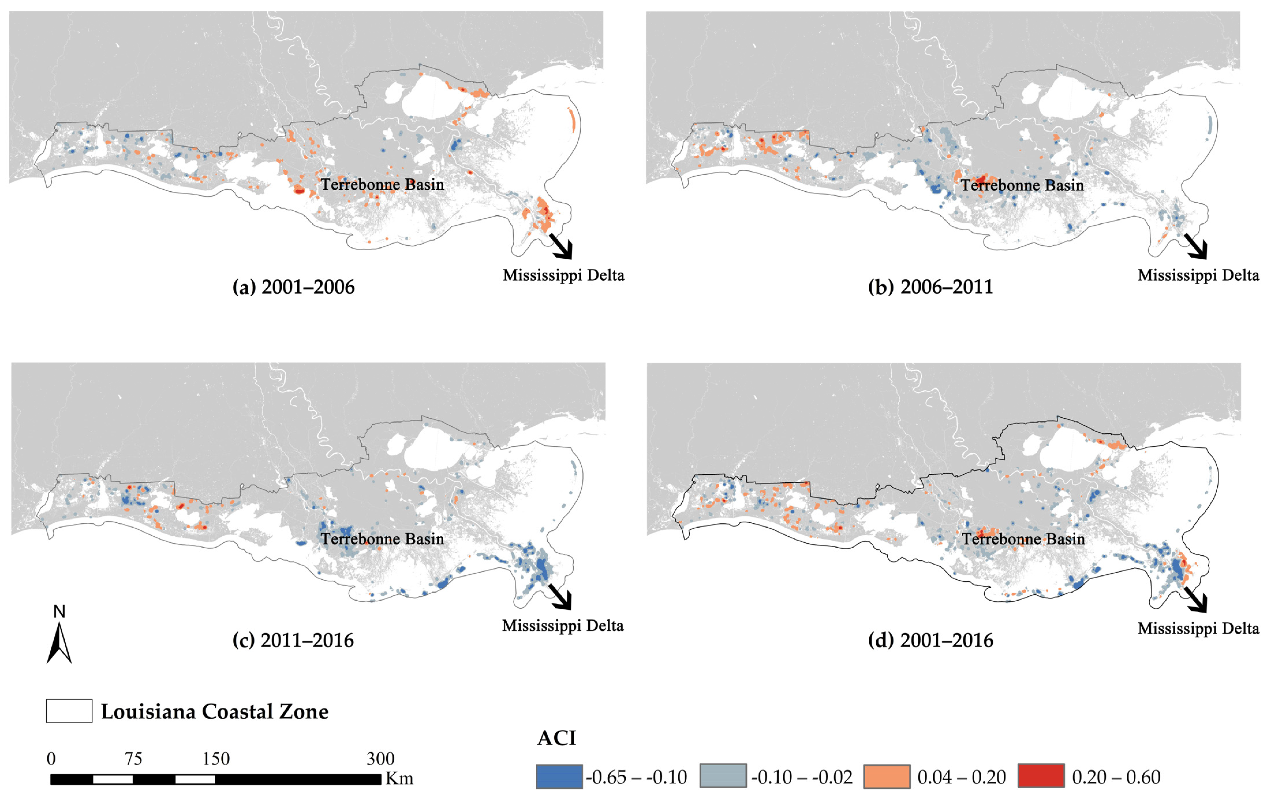
5.1. Spatial and Temporal Patterns of Land Change
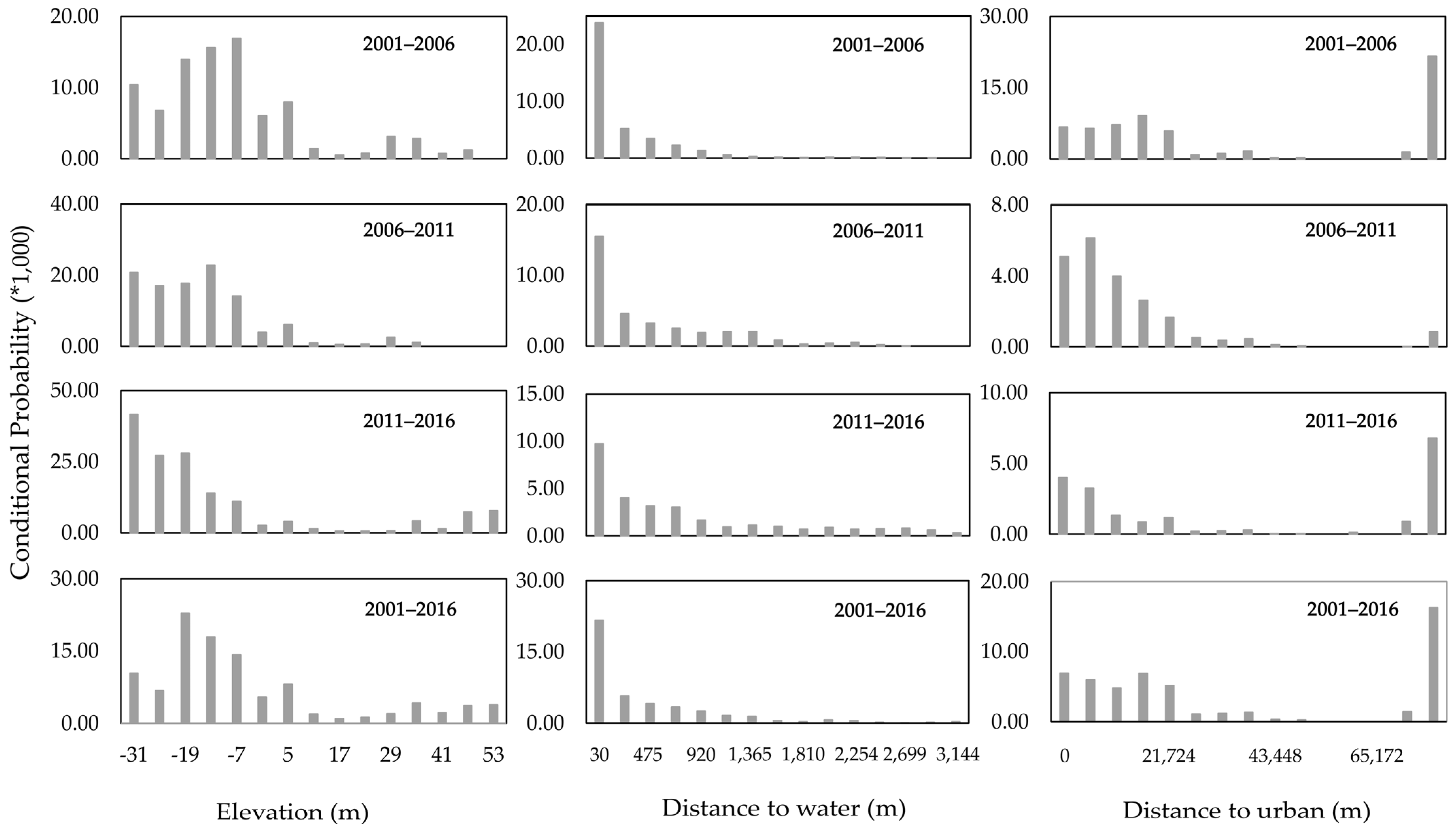
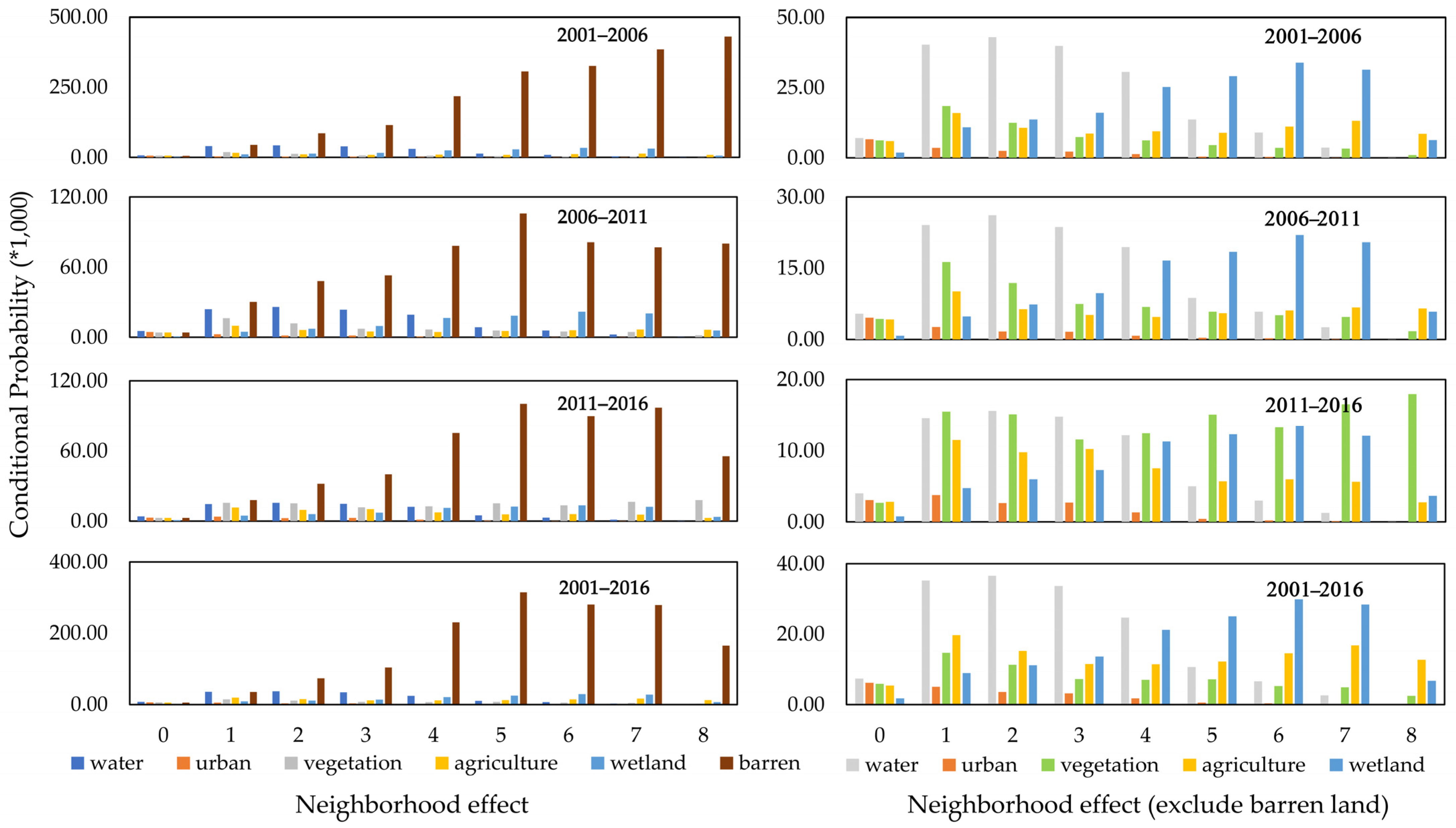
5.2. The Relationship between Land Loss and Selected Variables
5.3. Model Comparision
5.4. Models Explanation
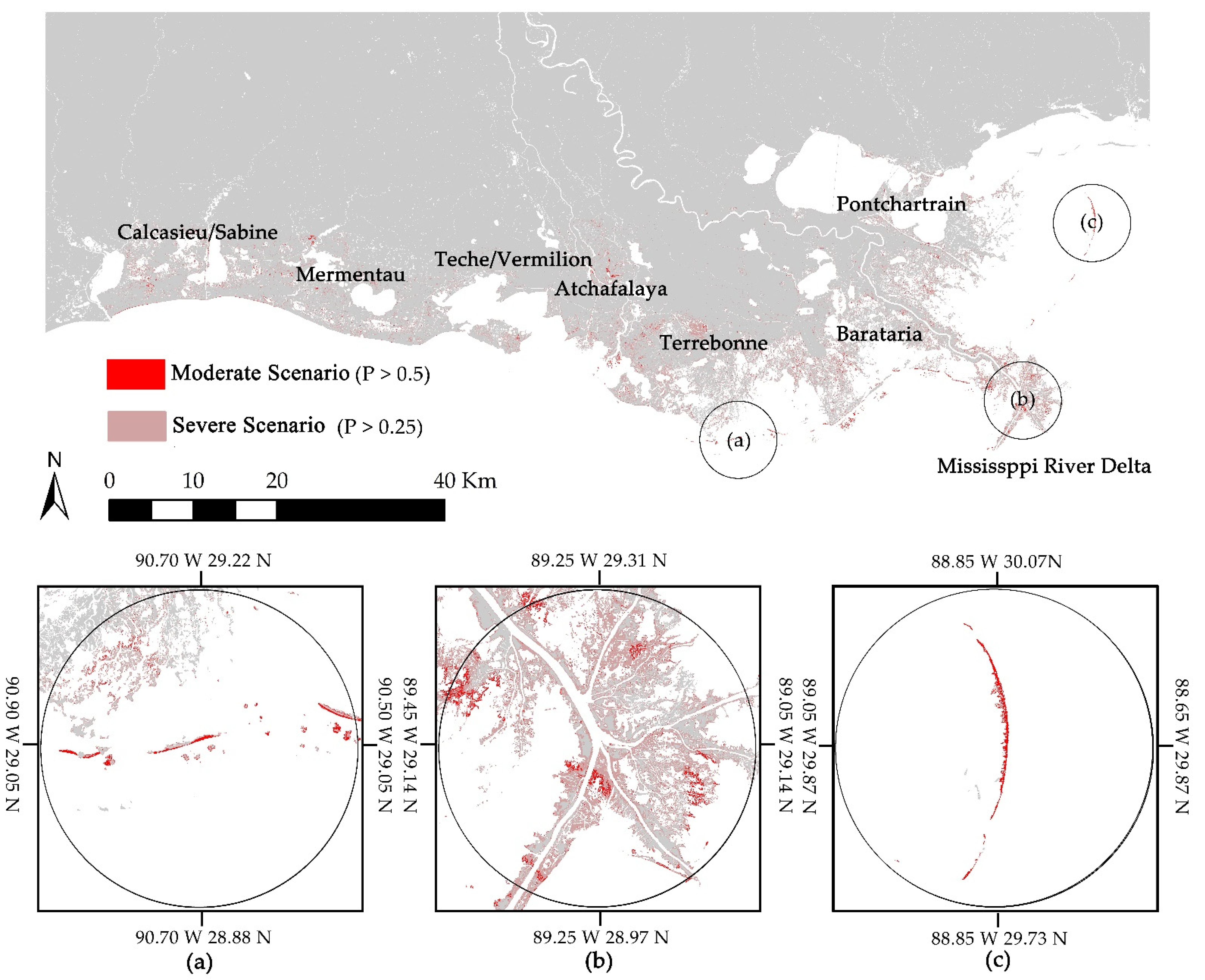
5.5. Land Loss Simulation and Prediction
6. Discussion and Conclusions
Author Contributions
Funding
Data Availability Statement
Conflicts of Interest
References
- Reed, D.; Wang, Y.; Meselhe, E.; White, E. Modeling wetland transitions and loss in coastal Louisiana under scenarios of future relative sea-level rise. Geomorphology 2019, 352, 106991. [Google Scholar] [CrossRef]
- Palaseanu-Lovejoy, M.; Kranenburg, C.; Barras, J.A.; Brock, J.C. Land Loss Due to Recent Hurricanes in Coastal Louisiana, USA. J. Coast. Res. 2013, 63, 97–109. [Google Scholar] [CrossRef]
- O’Leary, M.; Gottardi, R. Relationship between Growth Faults, Subsidence, and Land Loss: An Example from Cameron Parish, Southwestern Louisiana, USA. J. Coast. Res. 2020, 36, 812. [Google Scholar] [CrossRef]
- Mentaschi, L.; Vousdoukas, M.I.; Pekel, J.F.; Voukouvalas, E.; Feyen, L. Global long-term observations of coastal erosion and accretion. Sci. Rep. 2018, 8, 12876. [Google Scholar] [CrossRef] [Green Version]
- Barbier, E.B.; Georgiou, I.Y.; Enchelmeyer, B.; Reed, D.J. The Value of Wetlands in Protecting Southeast Louisiana from Hurricane Storm Surges. PLoS ONE 2013, 8, e58715. [Google Scholar] [CrossRef]
- Steyer, G.; Visser, J.; Owens, A.; Twilley, R. Coastal Louisiana Ecosystem Assessment and Restoration Program: The Role of Ecosystem Forecasting in Evaluating Restoration Planning in the Mississippi River Deltaic Plain. Trans. Am. Fish. Soc. 2008, 64, 29–46. [Google Scholar]
- Visser, J.M.; Duke-Sylvester, S.M.; Carter, J.; Broussard, W. A Computer Model to Forecast Wetland Vegetation Changes Resulting from Restoration and Protection in Coastal Louisiana. J. Coast. Res. 2013, 67, 51–59. [Google Scholar] [CrossRef]
- Colten, C.E. Environmental management in coastal Louisiana: A historical review. J. Coast. Res. 2017, 33, 699–711. [Google Scholar]
- Haer, T.; Kalnay, E.; Kearney, M.; Moll, H. Relative sea-level rise and the conterminous United States: Consequences of potential land inundation in terms of population at risk and GDP loss. Glob. Environ. Chang. 2013, 23, 1627–1636. [Google Scholar] [CrossRef]
- Hemmerling, S.; Carruthers, T.; Hijuelos, A.; Bienn, H. Double exposure and dynamic vulnerability: Assessing economic well-being, ecological change and the development of the oil and gas industry in coastal Louisiana. Shore Beach 2020, 72–82. [Google Scholar] [CrossRef]
- Tibbetts, J. Louisiana’s Wetlands: A Lesson in Nature Appreciation. Environ. Health Perspect. 2006, 114. [Google Scholar] [CrossRef]
- Roy, S.; Robeson, S.M.; Ortiz, A.C.; Edmonds, D.A. Spatial and temporal patterns of land loss in the Lower Mississippi River Delta from 1983 to 2016. Remote Sens. Environ. 2020, 250, 112046. [Google Scholar] [CrossRef]
- Coastal Protection and Restoration Authority of Louisiana. 2017. Louisiana’s Comprehensive Master Plan for a Sustainable Coast. Available online: http://coastal.la.gov/wp-content/uploads/2017/04/2017-Coastal-Master-Plan_Web-Book_CFinal-with-Effective-Date-06092017.pdf (accessed on 15 November 2021).
- Couvillion, B.R.; Beck, H.; Schoolmaster, D.; Fischer, M. Land area change in coastal Louisiana (1932 to 2016). U.S. Geol. Surv. 2017, 3381, 16. [Google Scholar] [CrossRef] [Green Version]
- Killebrew, C.J.; Khalil, S.M. An overview of history of coastal restoration plans and programs in Louisiana. Shore Beach 2018, 86, 28–37. [Google Scholar]
- Colten, C.E. Cartographic Depictions of Louisiana Land Loss: A Tool for Sustainable Policies. Sustainability 2018, 10, 763. [Google Scholar] [CrossRef] [Green Version]
- Qiang, Y.; Lam, N.S.N. Modeling land use and land cover changes in a vulnerable coastal region using artificial neural networks and cellular automata. Environ. Monit. Assess. 2015, 187, 57. [Google Scholar] [CrossRef] [PubMed]
- Zou, L.; Kent, J.; Lam, N.S.N.; Cai, H.; Qiang, Y.; Li, K. Evaluating Land Subsidence Rates and Their Implications for Land Loss in the Lower Mississippi River Basin. Water 2015, 8, 10. [Google Scholar] [CrossRef] [Green Version]
- Glick, P.; Clough, J.; Polaczyk, A.; Couvillion, B.; Nunley, B. Potential Effects of Sea-Level Rise on Coastal Wetlands in Southeastern Louisiana. J. Coast. Res. 2013, 63, 211–233. [Google Scholar] [CrossRef]
- Olea, R.A.; Coleman, J.L., Jr. A synoptic examination of causes of land loss in southern Louisiana as related to the exploitation of subsurface geologic resources. J. Coast. Res. 2014, 30, 1025–1044. [Google Scholar] [CrossRef]
- Lam, N.S.N.; Cheng, W.; Zou, L.; Cai, H. Effects of landscape fragmentation on land loss. Remote Sens. Environ. 2018, 209, 253–262. [Google Scholar] [CrossRef]
- Altinay, Z.; Rittmeyer, E.; Morris, L.L.; Reams, M.A. Public risk salience of sea level rise in Louisiana, United States. J. Environ. Stud. Sci. 2020, 11, 523–536. [Google Scholar] [CrossRef]
- Day, J.W.; Templet, P. Consequences of sea level rise: Implications from the Mississippi Delta. Coast. Manag. 1989, 17, 241–257. [Google Scholar] [CrossRef]
- FitzGerald, D.; Kulp, M.; Hughes, Z.; Georgiou, I.; Miner, M.; Penland, S.; Howes, N. Impacts of Rising Sea Level to Backbarrier Wetlands, Tidal Inlets, and Barrier Islands: Barataria Coast, Louisiana. Proc. Coast. Sediments 2007, 7, 1179–1192. [Google Scholar] [CrossRef]
- Jankowski, K.L.; Törnqvist, T.E.; Fernandes, A.M. Vulnerability of Louisiana’s coastal wetlands to present-day rates of relative sea-level rise. Nat. Commun. 2017, 8, 14792. [Google Scholar] [CrossRef] [Green Version]
- Day, J.W.; Shaffer, G.P.; Cahoon, D.R.; De Laune, R.D. Canals, backfilling and wetland loss in the Mississippi Delta. Estuarine Coast. Shelf Sci. 2019, 227, 106325. [Google Scholar] [CrossRef]
- Cahoon, D.R.; Lynch, J.C.; Roman, C.T.; Schmit, J.P.; Skidds, D.E. Evaluating the Relationship Among Wetland Vertical Development, Elevation Capital, Sea-Level Rise, and Tidal Marsh Sustainability. Estuaries Coasts 2018, 42, 1–15. [Google Scholar] [CrossRef]
- Jin, S.; Homer, C.; Yang, L.; Danielson, P.; Dewitz, J.; Li, C.; Zhu, Z.; Xian, G.; Howard, D. Overall Methodology Design for the United States National Land Cover Database 2016 Products. Remote Sens. 2019, 11, 2971. [Google Scholar] [CrossRef] [Green Version]
- Choi, W.; Deal, B.M. Assessing hydrological impact of potential land use change through hydrological and land use change modeling for the Kishwaukee River basin (USA). J. Environ. Manag. 2008, 88, 1119–1130. [Google Scholar] [CrossRef]
- Hu, T.; Liu, J.; Zheng, G.; Zhang, D.; Huang, K. Evaluation of historical and future wetland degradation using remote sensing imagery and land use modeling. Land Degrad. Dev. 2019, 31, 65–80. [Google Scholar] [CrossRef]
- Wickham, J.; Stehman, S.V.; Homer, C.G. Spatial patterns of the United States National Land Cover Dataset (NLCD) land-cover change thematic accuracy (2001–2011). Int. J. Remote Sens. 2017, 39, 1729–1743. [Google Scholar] [CrossRef] [Green Version]
- Anderson, J.R.; Hardy, E.E.; Roach, J.T.; Witmer, R.E. A Land Use and Land Cover Classification System for Use with Remote Sensor Data; Geological Survey Professional Paper 964; United States Department of the Interior: Washington, DC, USA, 1976.
- Ortiz, A.C.; Roy, S.; Edmonds, D.A. Land loss by pond expansion on the Mississippi River Delta Plain. Geophys. Res. Lett. 2017, 44, 3635–3642. [Google Scholar] [CrossRef]
- Day, J.W., Jr.; Boesch, D.F.; Clairain, E.J.; Kemp, G.P.; Laska, S.B.; Mitsch, W.J.; Orth, K.; Mashriqui, H.; Reed, D.J.; Shabman, L.; et al. Restoration of the Mississippi Delta: Lessons from Hurricanes Katrina and Rita. Science 2007, 315, 1679–1684. [Google Scholar] [CrossRef] [Green Version]
- Chambers, L.G.; Steinmuller, H.E.; Breithaupt, J.L. Toward a mechanistic understanding of “peat collapse” and its potential contribution to coastal wetland loss. Ecology 2019, 100, e02720. [Google Scholar] [CrossRef] [Green Version]
- Scavia, D.; Field, J.C.; Boesch, D.F.; Buddemeier, R.W.; Burkett, V.; Cayan, D.R.; Fogarty, M.; Harwell, M.A.; Howarth, R.; Mason, C.; et al. Climate change impacts on U.S. Coastal and Marine Ecosystems. Estuaries 2002, 25, 149–164. [Google Scholar] [CrossRef]
- González, J.L.; Tornqvist, T.E. Coastal Louisiana in crisis: Subsidence or sea level rise? Eos Trans. Am. Geophys. Union 2006, 87, 493–498. [Google Scholar] [CrossRef] [Green Version]
- Overmars, K.; de Koning, G.; Veldkamp, T. Spatial autocorrelation in multi-scale land use models. Ecol. Model. 2003, 164, 257–270. [Google Scholar] [CrossRef]
- Wear, D.N.; Bolstad, P. Land-use changes in southern Appalachian landscapes: Spatial analysis and forecast evaluation. Ecosystems 1998, 1, 575–594. [Google Scholar] [CrossRef] [Green Version]
- Bi, X.; Wang, B.; Lu, Q. Fragmentation effects of oil wells and roads on the Yellow River Delta, North China. Ocean Coast. Manag. 2011, 54, 256–264. [Google Scholar] [CrossRef]
- Feng, Y.; Liu, Y. A heuristic cellular automata approach for modelling urban land-use change based on simulated annealing. Int. J. Geogr. Inf. Sci. 2013, 27, 449–466. [Google Scholar] [CrossRef]
- Cowan, J.H., Jr.; Turner, R.E. Modeling wetland loss in coastal Louisiana: Geology, geography, and human modifications. Environ. Manag. 1988, 12, 827–838. [Google Scholar] [CrossRef]
- Rahman, H.A.A.; Wah, Y.B.; He, H.; Bulgiba, A. Comparisons of ADABOOST, KNN, SVM and Logistic Regression in Classification of Imbalanced Dataset; Springer: Singapore, 2015; pp. 54–64. [Google Scholar] [CrossRef]
- Cai, H.; Lam, N.S.N.; Zou, L.; Qiang, Y. Modeling the Dynamics of Community Resilience to Coastal Hazards Using a Bayesian Network. Ann. Am. Assoc. Geogr. 2018, 108, 1260–1279. [Google Scholar] [CrossRef]
- Breiman, L. Random forests. Mach. Learn. 2001, 45, 5–32. [Google Scholar] [CrossRef] [Green Version]
- Kamusoko, C.; Gamba, J. Simulating Urban Growth Using a Random Forest-Cellular Automata (RF-CA) Model. ISPRS Int. J. Geo-Inf. 2015, 4, 447–470. [Google Scholar] [CrossRef]
- Liaw, A.; Wiener, M. Classification and regression by RandomForest. R News 2002, 2, 18–22. [Google Scholar]
- Chen, T.; Guestrin, C. Xgboost: A scalable tree boosting system. In Proceedings of the 22nd ACM SIGKDD International Conference on Knowledge Discovery and Data Mining, San Francisco, CA, USA, 13–17 August 2016. [Google Scholar]
- Fan, J.; Upadhye, S.; Worster, A. Understanding receiver operating characteristic (ROC) curves. Can. J. Emerg. Med. 2006, 8, 19–20. [Google Scholar] [CrossRef] [PubMed]
- Goutte, C.; Gaussier, E. A probabilistic interpretation of precision, recall and F-score, with implication for evaluation. In European Conference on Information Retrieval; Springer: Berlin, Germany, 2005; pp. 345–359. [Google Scholar]
- Barras, J.; Beville, S.; Britsch, D.; Hartley, S.; Hawes, S.; Johnston, J.; Kemp, P.; Kinler, Q.; Martucci, A.; Porthouse, J.; et al. Historical and Projected Coastal Louisiana Land Changes: 1978–2050; United States Geological Survey Open File Report: Reston, VA, USA, 2003.
- McKee, K.L.; Cherry, J.A. Hurricane Katrina sediment slowed elevation loss in subsiding brackish marshes of the Mississippi River delta. Wetlands 2009, 29, 2–15. [Google Scholar] [CrossRef]
- Boyer, T.; Polasky, S. Valuing urban wetlands: A review of non-market valuation studies. Wetlands 2004, 24, 744–755. [Google Scholar] [CrossRef]
- Rojas, C.; Munizaga, J.; Rojas, O.; Martínez, C.; Pino, J. Urban development versus wetland loss in a coastal Latin American city: Lessons for sustainable land use planning. Land Use Policy 2018, 80, 47–56. [Google Scholar] [CrossRef]


| Original Land Cover | Anderson’s Land Cover Classification | Land/Water Categories |
|---|---|---|
| Water | Water | Water |
| Developed, Open Space | Urban | Land |
| Developed, Low Intensity | ||
| Developed, Medium Intensity | ||
| Developed, High Intensity | ||
| Barren Land | Barren | |
| Deciduous Forest | Vegetation | |
| Evergreen Forest | ||
| Mixed Forest | ||
| Shrub/Scrub | ||
| Herbaceuous | ||
| Hay/Pasture | Agriculture | |
| Cultivated Crop | ||
| Woody Wetlands | Wetlands | |
| Emergent Herbaceuous Wetlands |
| Variables | Data Source | Original Format |
|---|---|---|
| Environment | ||
| Elevation | SRTM 1 Arc-Second Global from US Geological Survey | Raster (30 m × 30 m) |
| Soil type | National Cooperative Soil Survey and supersedes the State Soil Geographic | Polygon |
| Subsidence rate | NOAA’s National Geodetic Survey, recorded from 1920 | Point |
| Original land cover | NOAA Coastal Service Center, updated in 2001, 2006, 2011 and 2016 | Raster (30 m × 30 m) |
| Moran’s I | Same as above | Same as above |
| Distance to water | Same as above | Same as above |
| Neighborhood Conditions | ||
| Number of water cells | NOAA Coastal Service Center, updated in 2001, 2006, 2011 and 2016 | Raster (30 m × 30 m) Neighborhood size: 3 × 3 cells |
| Number of urban cells | ||
| Number of barren cells | ||
| Number of vegetation cells | ||
| Number of agriculture cells | ||
| Number of wetland cells | ||
| Human Activity | ||
| Oil/gas well density | Louisiana Department of Natural Resource | Point |
| Distance to road | US Census Bureau, updated in 2000, 2006, 2011 and 2016 | Polyline |
| Distance to urban | NOAA Coastal Service Center, updated in 2001, 2006, 2011 and 2016 | Raster (30 m × 30 m) |
| Model | Parameter | Range | Optimum Value |
|---|---|---|---|
| RF | n_estimators | 400 to 1200 | 800 |
| max_feature | [Auto, SQRT, Log2] | Auto | |
| min_samples_split | [2, 4, 8] | 2 | |
| Bootstrap | [True, False] | FALSE | |
| XGBoost | Nrounds | 100 to 500 | 400 |
| Eta | 0 to 1 | 0.3 | |
| Gamma | 0 to 1 | 0 | |
| min_child_weight | 0 to 10 | 1 |
| 2001–2006 | 2006–2011 | 2011–2016 | 2001–2016 | |||||||||
|---|---|---|---|---|---|---|---|---|---|---|---|---|
| LR | XGBoost | RF | LR | XGBoost | RF | LR | XGBoost | RF | LR | XGBoost | RF | |
| AUC | 0.73 | 0.86 | 0.93 | 0.70 | 0.87 | 0.95 | 0.72 | 0.85 | 0.92 | 0.75 | 0.87 | 0.95 |
| Accuracy | 0.76 | 0.89 | 0.89 | 0.75 | 0.90 | 0.90 | 0.75 | 0.89 | 0.88 | 0.76 | 0.91 | 0.91 |
| Precision | 0.69 | 0.84 | 0.85 | 0.62 | 0.86 | 0.86 | 0.64 | 0.84 | 0.83 | 0.63 | 0.88 | 0.88 |
| Recall | 0.32 | 0.77 | 0.75 | 0.31 | 0.79 | 0.78 | 0.25 | 0.76 | 0.72 | 0.20 | 0.75 | 0.74 |
| F1-score | 0.44 | 0.80 | 0.80 | 0.41 | 0.82 | 0.82 | 0.36 | 0.80 | 0.77 | 0.30 | 0.80 | 0.80 |
| 2001–2006 | 2006–2011 | 2011–2016 | 2001–2016 | |
|---|---|---|---|---|
| Elevation | −4.63 | −5.07 | −6.19 | −4.30 |
| Number of urban cells | −4.10 | −4.73 | −2.68 | −3.71 |
| Distance to water area | −2.55 | −1.98 | −1.56 | −2.42 |
| Oil/gas well density | +0.27 | −1.68 | −1.76 | −1.14 |
| Distance to urban area | +0.28 | −2.56 | −3.17 | −0.28 |
| Moran’s I | +0.19 | +0.26 | −0.27 | +0.61 |
| Number of vegetation cells | +0.79 | +1.29 | +2.65 | +1.05 |
| Number of water cells | +1.27 | +1.57 | +1.78 | +1.06 |
| Number of agriculture cells | +1.15 | +0.88 | +0.73 | +1.55 |
| Subsidence rate | +1.76 | +4.37 | +1.28 | +2.16 |
| Number of barren cells | +4.34 | +3.11 | +4.87 | +4.15 |
| 2001–2006 | 2006–2011 | 2011–2016 | 2001–2016 | |
|---|---|---|---|---|
| Oil/well gas density | +1.66 | +0.98 | +0.13 | +0.46 |
| Moran’s I | +1.25 | +0.50 | +0.15 | +1.14 |
| Distances to urban | +2.21 | −0.08 | −0.55 | +1.49 |
| Probability of Land Loss | The Number of Pixels | Area (km2) |
|---|---|---|
| 0–10% | 4,662,297 | 4196.07 |
| 10–20% | 3,036,637 | 2732.97 |
| 20–30% | 2,195,063 | 1975.56 |
| 30–40% | 1,318,586 | 1186.73 |
| 40–50% | 436,932 | 393.24 |
| 50–60% | 127,998 | 115.20 |
| 60–70% | 52,131 | 46.92 |
| 70–80% | 11,735 | 10.56 |
| 80–90% | 556 | 0.50 |
| 90–100% | 8 | 0.01 |
Publisher’s Note: MDPI stays neutral with regard to jurisdictional claims in published maps and institutional affiliations. |
© 2022 by the authors. Licensee MDPI, Basel, Switzerland. This article is an open access article distributed under the terms and conditions of the Creative Commons Attribution (CC BY) license (https://creativecommons.org/licenses/by/4.0/).
Share and Cite
Yang, M.; Zou, L.; Cai, H.; Qiang, Y.; Lin, B.; Zhou, B.; Abedin, J.; Mandal, D. Spatial–Temporal Land Loss Modeling and Simulation in a Vulnerable Coast: A Case Study in Coastal Louisiana. Remote Sens. 2022, 14, 896. https://doi.org/10.3390/rs14040896
Yang M, Zou L, Cai H, Qiang Y, Lin B, Zhou B, Abedin J, Mandal D. Spatial–Temporal Land Loss Modeling and Simulation in a Vulnerable Coast: A Case Study in Coastal Louisiana. Remote Sensing. 2022; 14(4):896. https://doi.org/10.3390/rs14040896
Chicago/Turabian StyleYang, Mingzheng, Lei Zou, Heng Cai, Yi Qiang, Binbin Lin, Bing Zhou, Joynal Abedin, and Debayan Mandal. 2022. "Spatial–Temporal Land Loss Modeling and Simulation in a Vulnerable Coast: A Case Study in Coastal Louisiana" Remote Sensing 14, no. 4: 896. https://doi.org/10.3390/rs14040896
APA StyleYang, M., Zou, L., Cai, H., Qiang, Y., Lin, B., Zhou, B., Abedin, J., & Mandal, D. (2022). Spatial–Temporal Land Loss Modeling and Simulation in a Vulnerable Coast: A Case Study in Coastal Louisiana. Remote Sensing, 14(4), 896. https://doi.org/10.3390/rs14040896