
Vegetation Monitoring of Protected Areas in Rugged Mountains Using an Improved Shadow-Eliminated Vegetation Index (SEVI)


Abstract
:
1. Introduction
2. Study Areas and Data
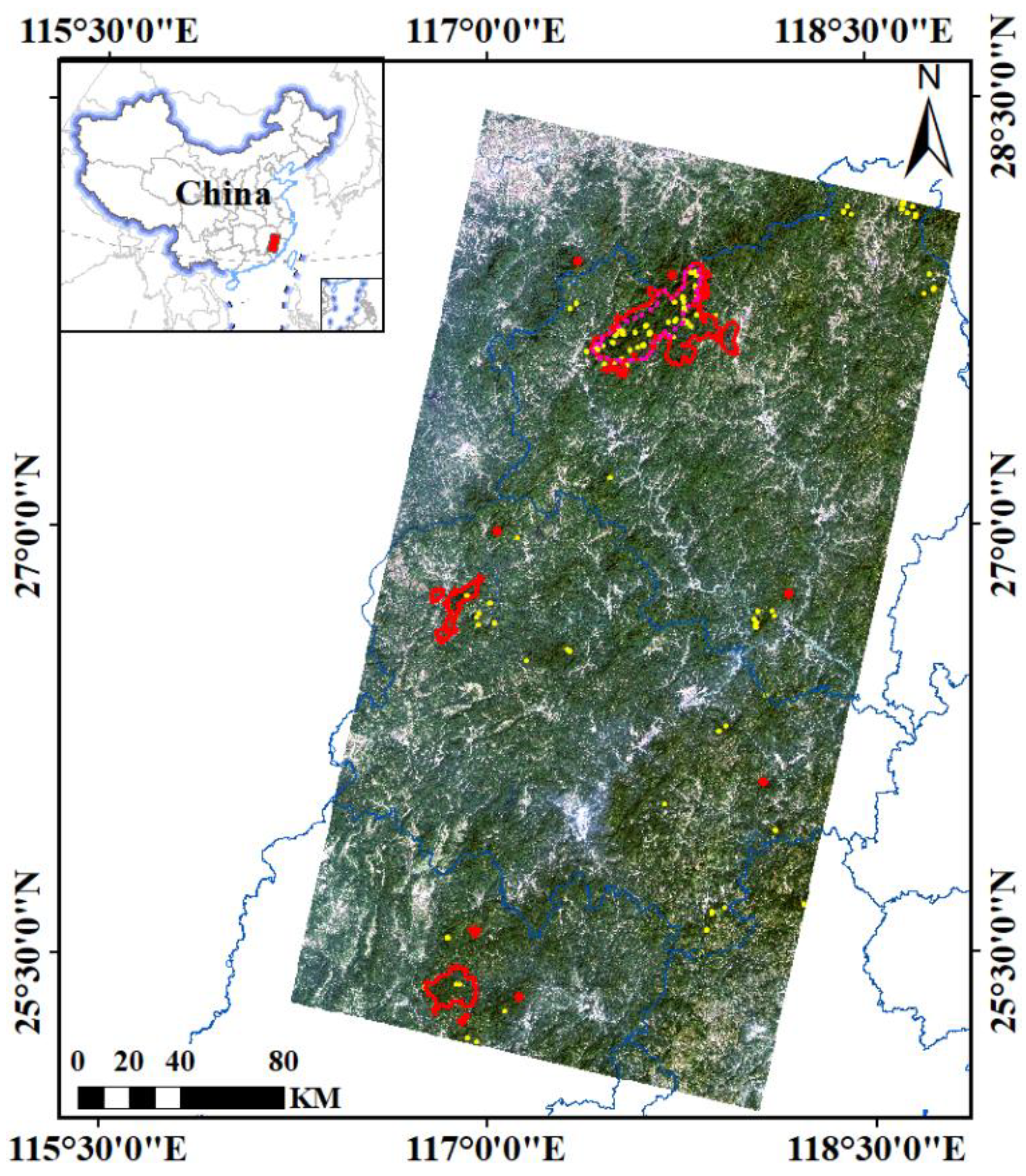
2.1. Study Areas
2.2. Data
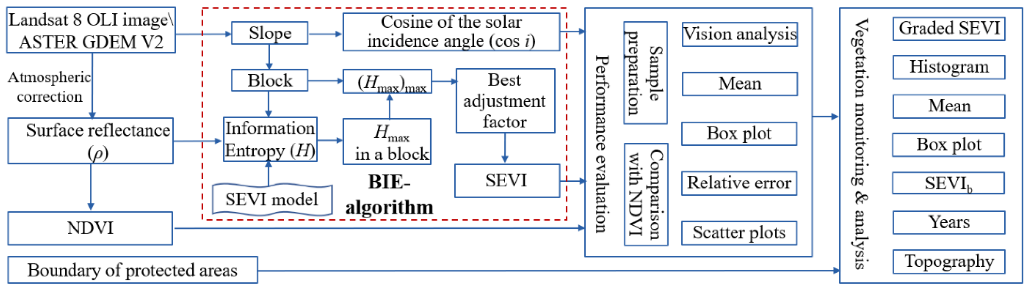
3. Methods
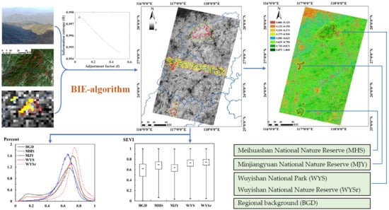
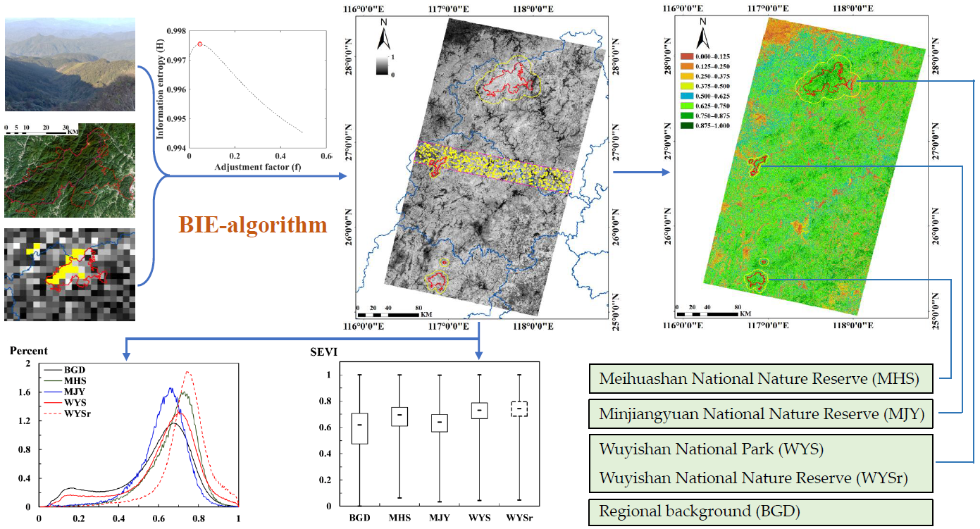
3.1. BIE-Algorithm Development
3.2. Performance Evaluation
3.3. Vegetation Monitoring and Analysis
4. Results
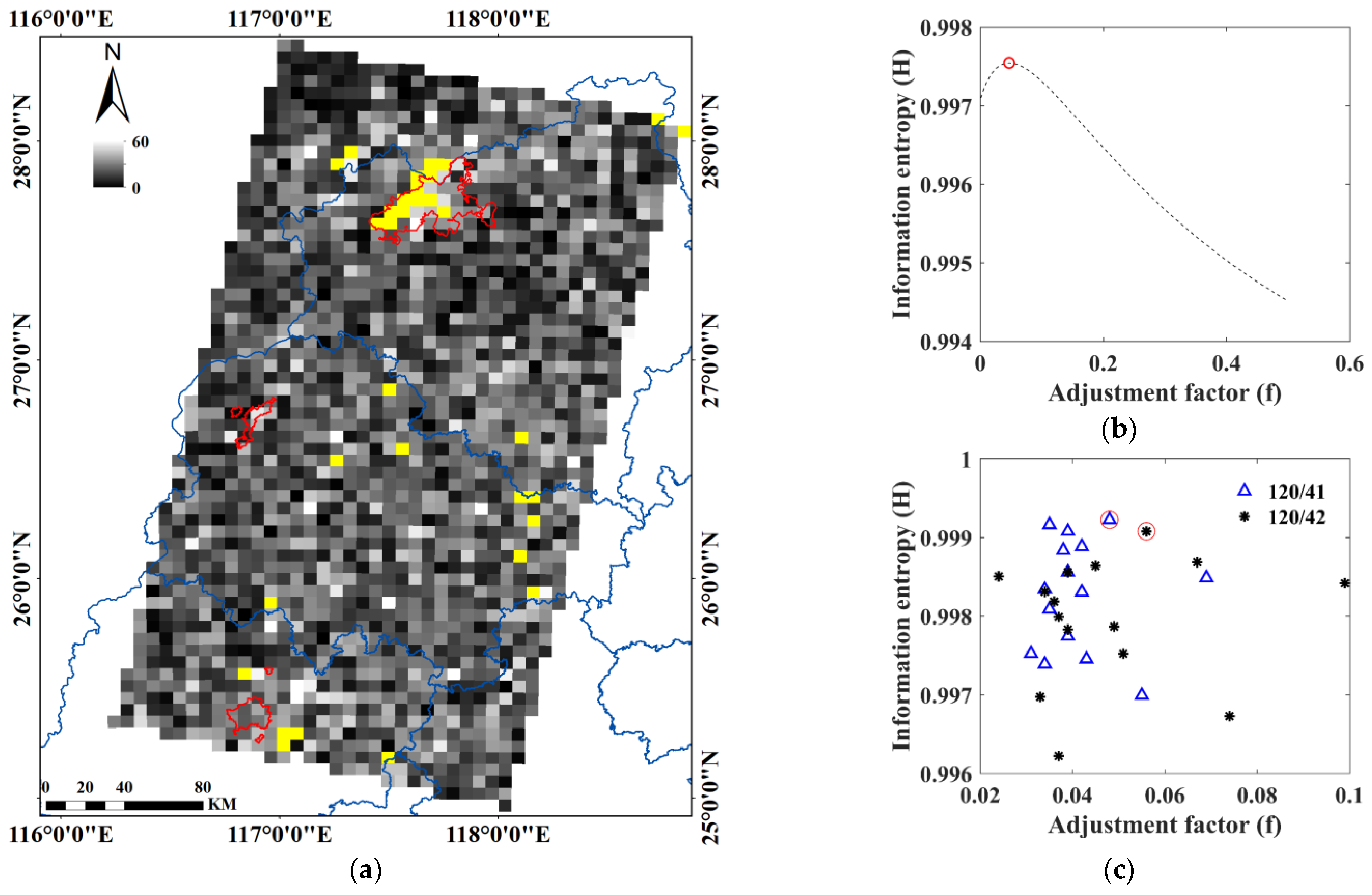
4.1. Block and Adjustment Factor
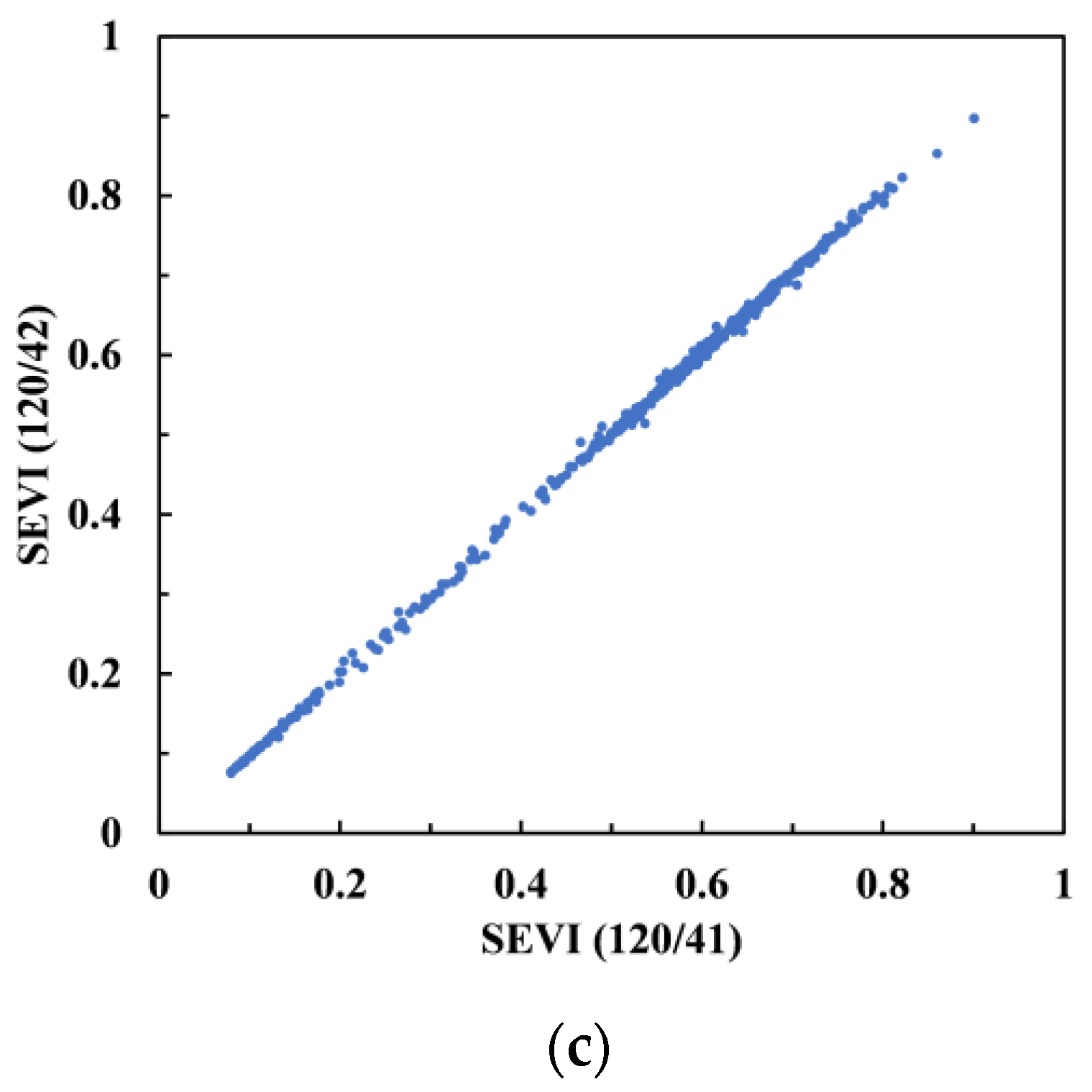
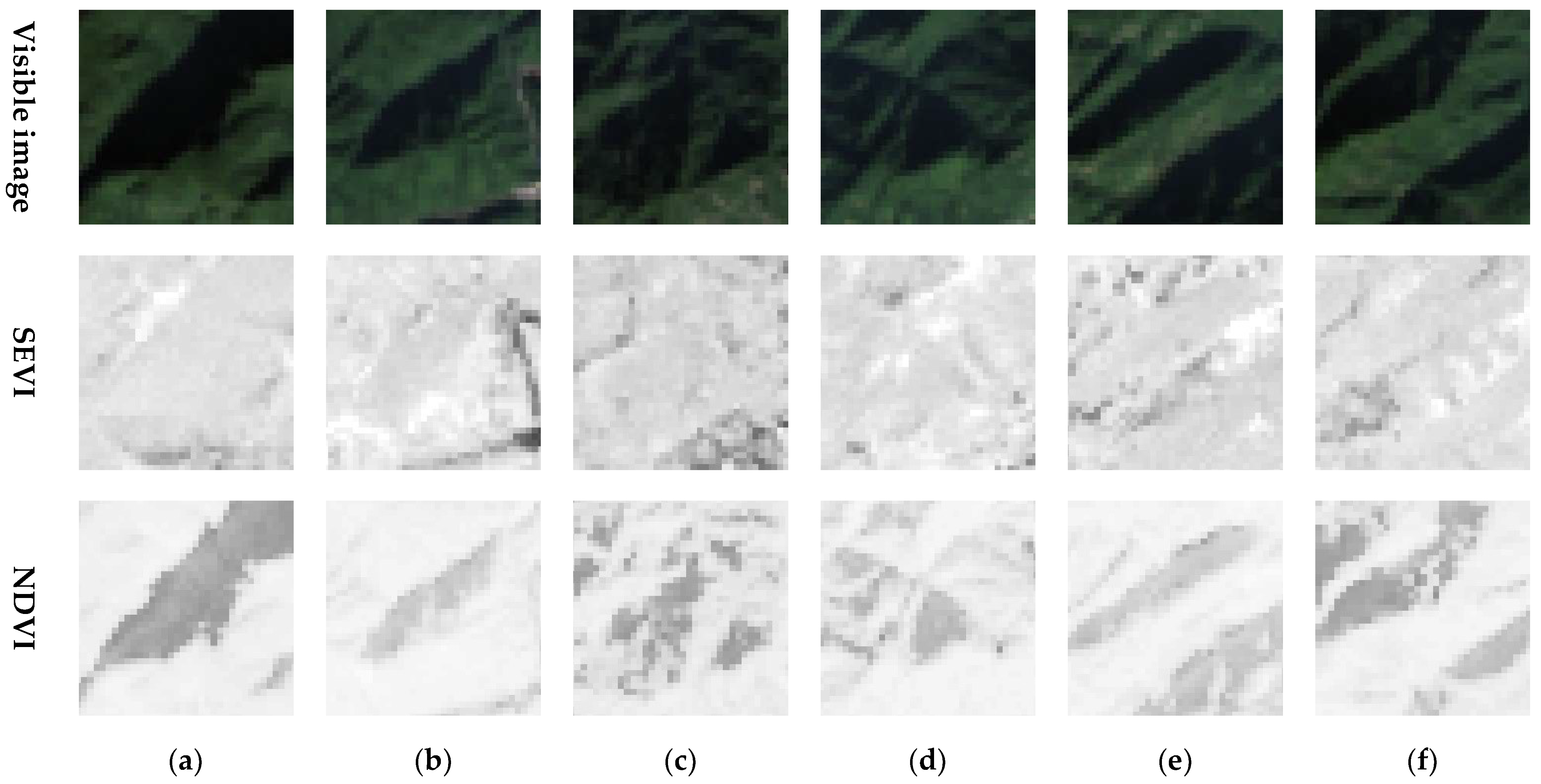
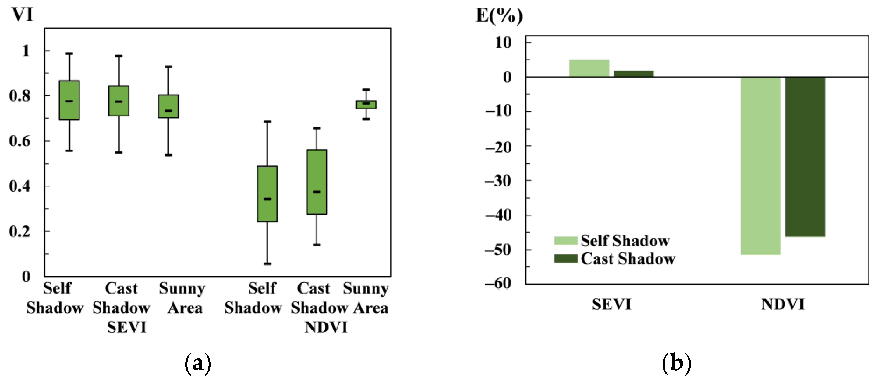
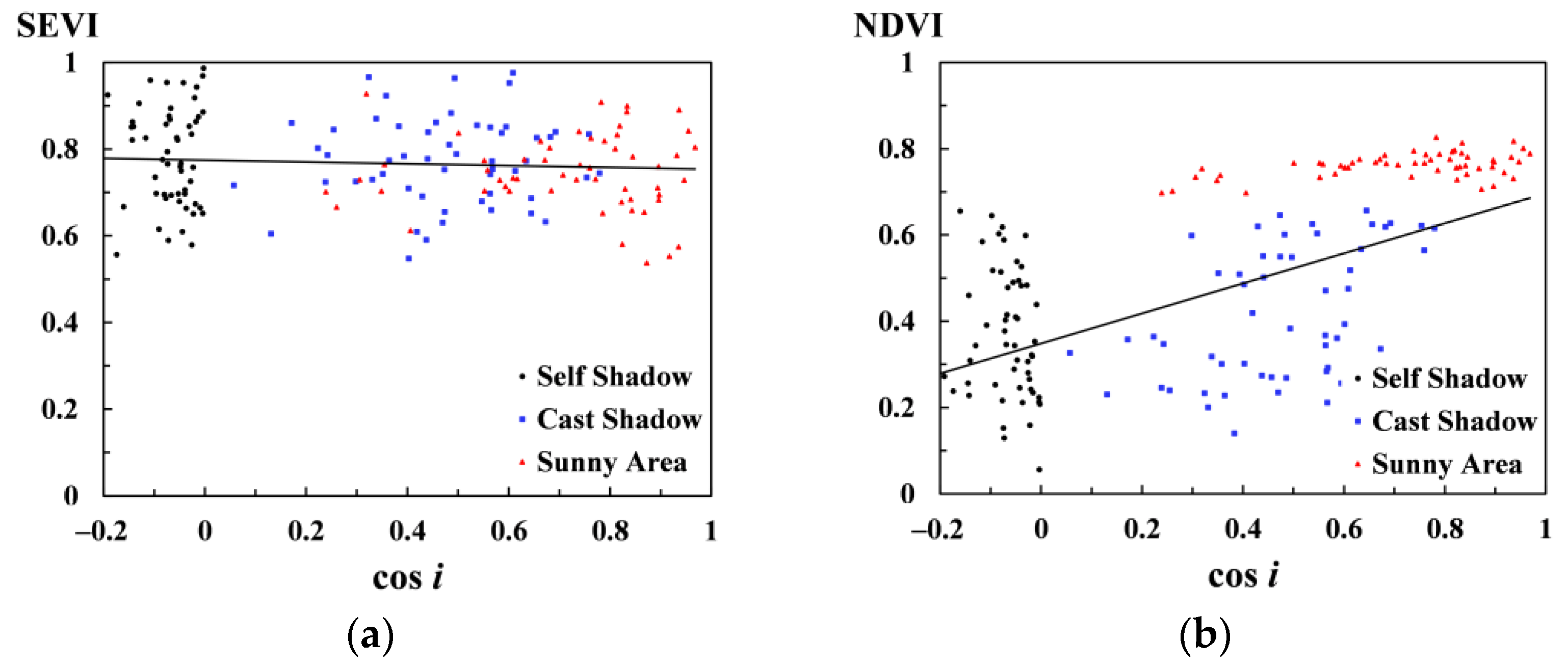
4.2. Performance of BIE-Algorithm
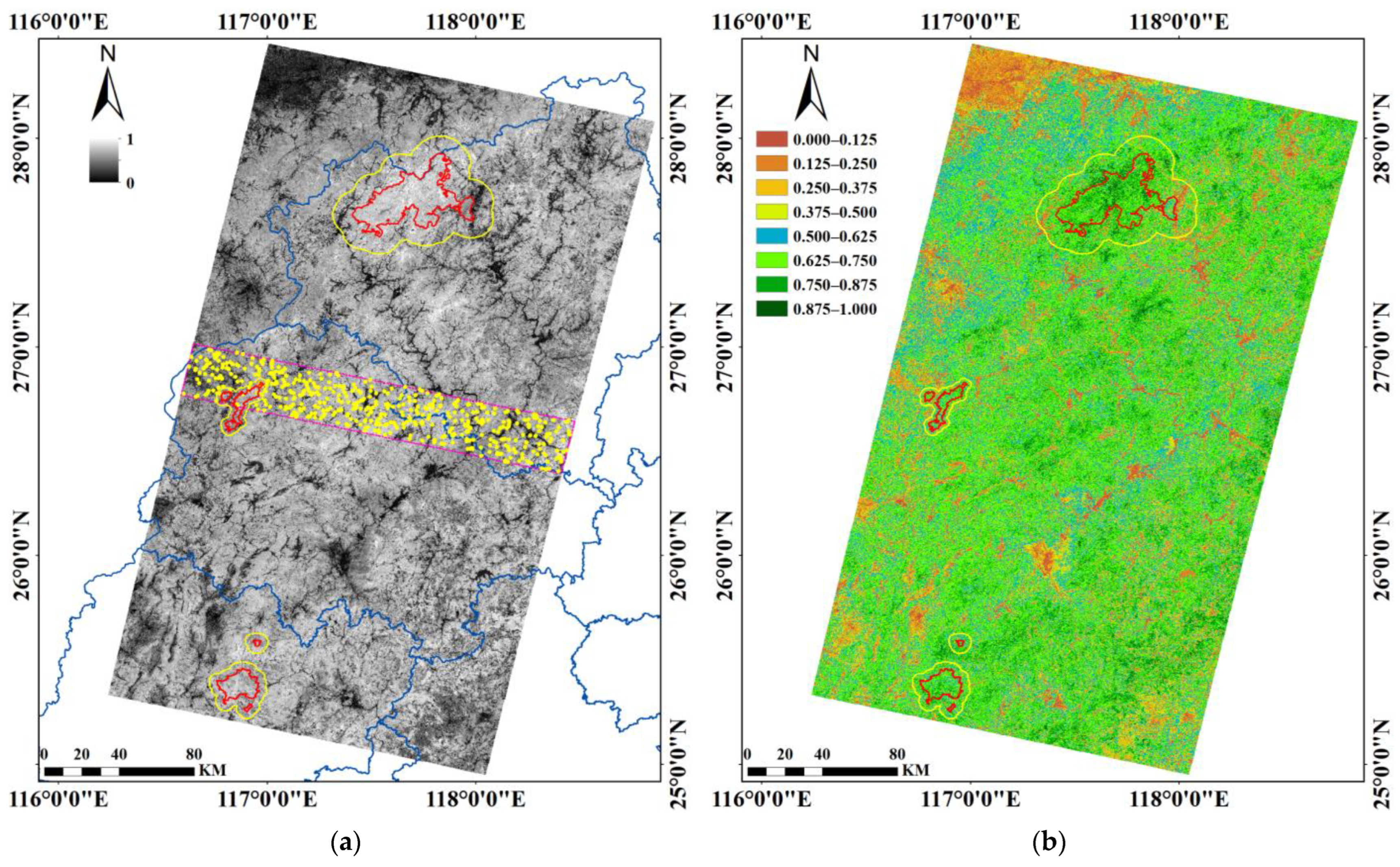
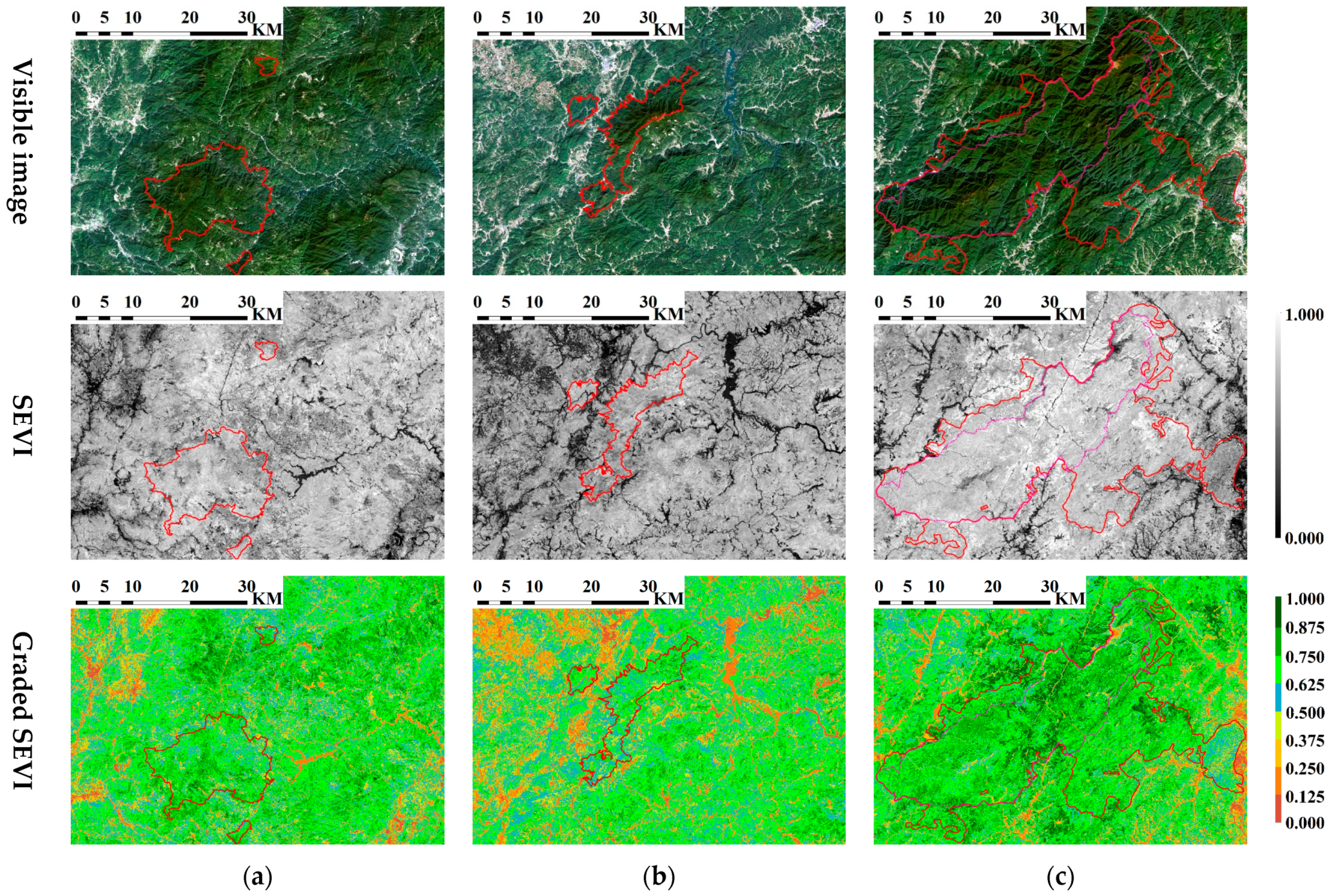
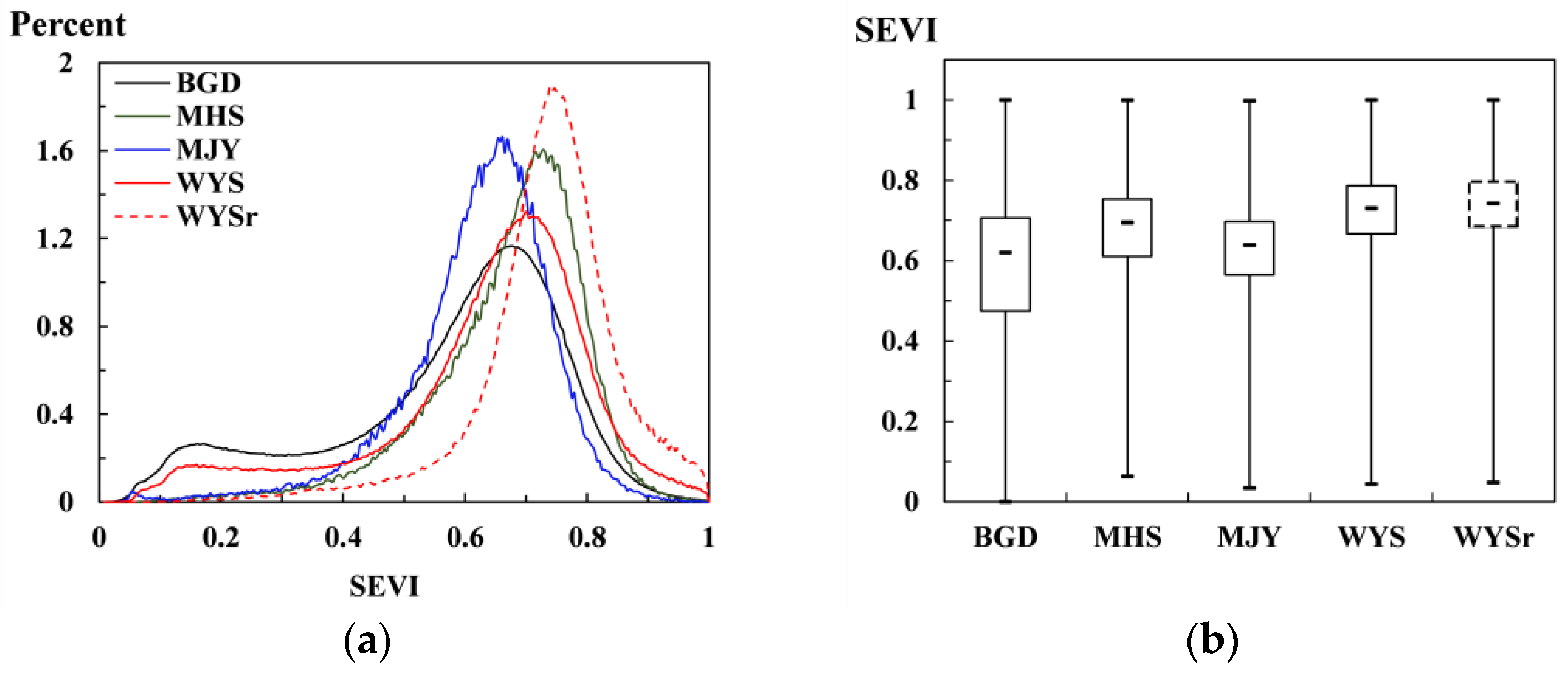
4.3. Vegetation Distribution
5. Discussion
5.1. BIE-Algorithm
5.2. SEVI Feature
5.3. Vegetation of Protected Areas
6. Conclusions
Author Contributions
Funding
Acknowledgments
Conflicts of Interest
References
- Pereira, H.M.; Leadley, P.W.; Proença, V.; Alkemade, R.; Scharlemann, J.P.W.; Fernandez-Manjarrés, J.F.; Araújo, M.B.; Balvanera, P.; Biggs, R.; Cheung, W.W.L.; et al. Scenarios for global biodiversity in the 21st century. Science 2010, 330, 1496–1501. [Google Scholar] [CrossRef] [PubMed] [Green Version]
- Bellassen, V.; Luyssaert, S. Carbon sequestration: Managing forests in uncertain times. Nature 2014, 506, 153–155. [Google Scholar] [CrossRef] [PubMed] [Green Version]
- Le Quéré, C.; Andrew, R.M.; Friedlingstein, P.; Sitch, S.; Hauck, J.; Pongratz, J.; Pickers, P.A.; Korsbakken, J.I.; Peters, G.P.; Canadell, J.G.; et al. Global carbon budget 2018. Earth Syst. Sci. Data 2018, 10, 2141–2194. [Google Scholar] [CrossRef] [Green Version]
- Di Marco, M.; Watson, J.E.M.; Currie, D.J.; Possingham, H.P.; Venter, O. The extent and predictability of the biodiversity-carbon correlation. Ecol. Lett. 2018, 21, 365–375. [Google Scholar] [CrossRef] [Green Version]
- Buřivalová, Z.; Hart, S.J.; Radeloff, V.C.; Srinivasan, U. Early warning sign of forest loss in protected areas. Curr. Biol. 2021, 31, 4620–4626. [Google Scholar] [CrossRef]
- Cao, M.; Peng, L.; Liu, S. Analysis of the network of protected areas in China based on a geographic perspective: Current status, issues and integration. Sustainability 2015, 7, 15617–15631. [Google Scholar] [CrossRef] [Green Version]
- Tang, J.; Lu, H.; Xue, Y.; Li, J.; Li, G.; Mao, Y.; Deng, C.; Li, D. Data-driven planning adjustments of the functional zoning of Houhe National Nature Reserve. Glob. Ecol. Conserv. 2021, 29, e01708. [Google Scholar] [CrossRef]
- Ding, Y.; Qiu, M. Research on establishing nature reserve system with national park as the main body: A case study of Potatso National Park system pilot area. Int. J. Geoherit. Parks 2020, 8, 239–243. [Google Scholar] [CrossRef]
- Fassnacht, F.E.; Latifi, H.; Koch, B. An angular vegetation index for imaging spectroscopy data—Preliminary results on forest damage detection in the Bavarian National Park, Germany. Int. J. Appl. Earth Obs. 2012, 19, 308–321. [Google Scholar] [CrossRef]
- Wang, G.; Wang, M.; Yuan, Y.; Lu, X.; Jiang, M. Effects of sediment load on the seed bank and vegetation of Calamagrostis angustifolia wetland community in the National Natural Wetland Reserve of Lake Xingkai, China. Ecol. Eng. 2014, 63, 27–33. [Google Scholar] [CrossRef]
- Powers, R.P.; Coops, N.C.; Nelson, T.; Wulder, M.A. Evaluating nature reserve design efficacy in the Canadian Boreal forest using time series AVHRR data. Can. J. Remote Sens. 2016, 42, 171–189. [Google Scholar] [CrossRef]
- Yu, B.; Chao, X.; Zhang, J.; Xu, W.; Ouyang, Z. Effectiveness of nature reserves for natural forests protection in tropical Hainan: A 20 year analysis. Chin. Geogr. Sci. 2016, 26, 208–215. [Google Scholar] [CrossRef] [Green Version]
- Hamadou, A.Z.; Hyacente, A.; Paul, K.; Danra, D.D.; Clautilde, M. Influence of anthropization on flora and the carbon stock of the corridor’s vegetation at the Benoue National Park of Cameroon. Environ. Chall. 2021, 5, 100345. [Google Scholar] [CrossRef]
- Mengist, W.; Soromessa, T.; Feyisa, G.L. Monitoring Afromontane forest cover loss and the associated socio-ecological drivers in Kaffa Biosphere Reserve, Ethiopia. Trees For. People 2021, 6, 100161. [Google Scholar] [CrossRef]
- Townshend, J.R.; Masek, J.G.; Huang, C.; Vermote, E.F.; Gao, F.; Channan, S.; Sexton, J.O.; Feng, M.; Narasimhan, R.; Kim, D.; et al. Global characterization and monitoring of forest cover using Landsat data: Opportunities and challenges. Int. J. Digit. Earth 2012, 5, 373–397. [Google Scholar] [CrossRef] [Green Version]
- Alphonse, K.; Alishir, K.; Felix, N.; Lamek, N.; Fidele, K.; Abdimijit, A.; Haiwen, L.; Osman, I. Monitoring forest cover change and fragmentation using remote sensing and landscape metrics in Nyungwe-Kibira park. J. Geosci. Environ. Prot. 2016, 4, 11–33. [Google Scholar]
- Da Ponte, E.; Mack, B.; Wohlfart, C.; Rodas, O.; Fleckenstein, M.; Oppelt, N.; Dech, S.; Kuenzer, C. Assessing forest cover dynamics and forest perception in the Atlantic forest of Paraguay, combining remote sensing and household level data. Forests 2017, 8, 389. [Google Scholar] [CrossRef] [Green Version]
- Garioud, A.; Valero, S.; Giordano, S.; Mallet, C. Recurrent-based regression of Sentinel time series for continuous vegetation monitoring. Remote Sens. Environ. 2021, 263, 112419. [Google Scholar] [CrossRef]
- Wulder, M.A.; Masek, J.G.; Cohen, W.B.; Loveland, T.R.; Woodcock, C.E. Opening the archive: How free data has enabled the science and monitoring promise of Landsat. Remote Sens. Environ. 2012, 122, 2–10. [Google Scholar] [CrossRef]
- Bai, Y. Analysis of vegetation dynamics in the Qinling-Daba Mountains region from MODIS time series data. Ecol. Indic. 2021, 129, 108029. [Google Scholar] [CrossRef]
- Hansen, M.C.; Potapov, P.V.; Moore, R.; Hancher, M.; Turubanova, S.A.; Tyukavina, A.; Thau, D.; Stehman, S.V.; Goetz, S.J.; Loveland, T.R.; et al. High-resolution global maps of 21st-century forest cover change. Science 2013, 342, 850–853. [Google Scholar] [CrossRef] [PubMed] [Green Version]
- Thapa, R.B.; Shimada, M.; Watanabe, M.; Motohka, T.; Shiraishi, T. The tropical forest in south east Asia: Monitoring and scenario modeling using synthetic aperture radar data. Appl. Geogr. 2013, 41, 168–178. [Google Scholar] [CrossRef]
- Silveira, E.M.O.; Radeloff, V.C.; Martinuzzi, S.; Pastur, G.J.M.; Rivera, L.O.; Politi, N.; Lizarraga, L.; Farwell, L.S.; Elsen, P.R.; Pidgeon, A.M. Spatio-temporal remotely sensed indices identify hotspots of biodiversity conservation concern. Remote Sens. Environ. 2021, 258, 112368. [Google Scholar] [CrossRef]
- Chance, C.M.; Hermosilla, T.; Coops, N.C.; Wulder, M.A.; White, J.C. Effect of topographic correction on forest change detection using spectral trend analysis of Landsat pixel-based composites. Int. J. Appl. Earth Obs. 2016, 44, 186–194. [Google Scholar] [CrossRef]
- Bishop, M.P.; Young, B.; Colby, J.; Furfaro, R.; Schiassi, E.; Chi, Z. Theoretical evaluation of anisotropic reflectance correction approaches for addressing multi-scale topographic effects on the radiation-transfer cascade in mountain environments. Remote Sens. 2019, 11, 2728. [Google Scholar] [CrossRef] [Green Version]
- Moreira, E.P.; Valeriano, M.M. Application and evaluation of topographic correction methods to improve land cover mapping using object-based classification. Int. J. Appl. Earth Obs. 2014, 32, 208–217. [Google Scholar] [CrossRef]
- Li, H.; Xu, L.; Shen, H.; Zhang, L. A general variational framework considering cast shadows for the topographic correction of remote sensing imagery. ISPRS Int. J. Geo-Inf. 2016, 117, 161–171. [Google Scholar] [CrossRef]
- Teillet, P.M.; Guindon, B.; Goodenough, D.G. On the slope-aspect correction of multispectral scanner data. Can. J. Remote Sens. 1982, 8, 84–106. [Google Scholar] [CrossRef] [Green Version]
- Civco, D.L. Topographic normalization of landsat thematic mapper digital imagery. Photogramm. Eng. Remote Sens. 1989, 55, 1303–1309. [Google Scholar]
- Meyer, P.; Itten, K.L.; Kellenberger, T.; Sandmeier, S.; Sandmeier, R. Radiometric corrections of topographically induced effects on Landsat TM data in an alpine environment. ISPRS J. Photogramm. Remote Sens. 1993, 48, 17–28. [Google Scholar] [CrossRef]
- Gu, D.; Gillespie, A. Topographic normalization of Landsat TM images of forest based on subpixel sun–canopy–sensor geometry. Remote Sens. Environ. 1998, 64, 166–175. [Google Scholar] [CrossRef]
- Riano, D.; Chuvieco, E.; Salas, J.; Aguado, I. Assessment of different topographic corrections in Landsat TM data for mapping vegetation types. IEEE Trans. Geosci. Remote Sens. 2003, 41, 1056–1061. [Google Scholar] [CrossRef] [Green Version]
- Soenen, S.A.; Peddle, D.R.; Coburn, C.A. SCS + C: A modified sun-canopy-sensor topographic correction in forested terrain. IEEE Trans. Geosci. Remote Sens. 2005, 43, 2148–2159. [Google Scholar] [CrossRef]
- Vázquez-Jiménez, R.; Romero-Calcerrada, R.; Ramos-Bernal, R.; Arrogante-Funes, P.; Novillo, C. Topographic correction to Landsat imagery through slope classification by applying the SCS + C Method in mountainous forest areas. ISPRS Int. J. Geo-Inf. 2017, 6, 287. [Google Scholar] [CrossRef]
- Smith, J.A.; Lin, T.L.; Ranson, K.J. The lambertian assumption and Landsat data. Photogramm. Eng. Remote Sens. 1980, 46, 1183–1189. [Google Scholar]
- Kane, V.; Gillespie, A.; McGaughey, R.; Lutz, J.; Ceder, K.; Franklin, J. Interpretation and topographic compensation of conifer canopy self-shadowing. Remote Sens. Environ. 2008, 112, 3820–3832. [Google Scholar] [CrossRef]
- Richter, R.; Kellenberger, T.; Kaufmann, H. Comparison of topographic correction methods. Remote Sens. 2009, 1, 184–196. [Google Scholar] [CrossRef] [Green Version]
- Sandmeier, S.; Itten, K.I. A physically-based model to correct atmospheric and illumination effects in optical satellite data of rugged terrain. IEEE Trans. Geosci. Remote Sens. 1997, 35, 708–717. [Google Scholar] [CrossRef] [Green Version]
- Santini, F.; Palombo, A. Physically based approach for combined atmospheric and topographic corrections. Remote Sens. 2019, 11, 1218. [Google Scholar] [CrossRef] [Green Version]
- Wen, J.; Liu, Q.; Liu, Q.; Xiao, Q.; Li, X. Parametrized BRDF for atmospheric and topographic correction and albedo estimation in Jiangxi rugged terrain, China. Int. J. Remote Sens. 2009, 30, 2875–2896. [Google Scholar] [CrossRef]
- Yin, G.; Li, A.; Wu, S.; Fan, W.; Zeng, Y.; Yan, K.; Xu, B.; Li, J.; Liu, Q. PLC: A simple and semi-physical topographic correction method for vegetation canopies based on path length correction. Remote Sens. Environ. 2018, 215, 184–198. [Google Scholar] [CrossRef]
- Chen, J.M.; Leblanc, S.G. A four-scale bidirectional reflectance model based on canopy architecture. IEEE Trans. Geosci. Remote Sens. 1997, 35, 1316–1337. [Google Scholar] [CrossRef]
- Fan, W.; Li, J.; Liu, Q.; Zhang, Q.; Yin, G.; Li, A.; Zeng, Y.; Xu, B.; Xu, X.; Zhou, G.; et al. Topographic correction of forest image data based on the canopy reflectance model for sloping terrains in multiple forward mode. Remote Sens. 2018, 10, 717. [Google Scholar] [CrossRef] [Green Version]
- Liao, Z.; He, B.; Quan, X. Modified enhanced vegetation index for reducing topographic effects. J. Appl. Remote Sens. 2015, 9, 096068. [Google Scholar] [CrossRef]
- Jiang, H.; Wang, S.; Cao, X.; Yang, C.; Zhang, Z.; Wang, X. A shadow-eliminated vegetation index (SEVI) for removal of self and cast shadow effects on vegetation in rugged terrains. Int. J. Digit. Earth 2019, 12, 1013–1029. [Google Scholar] [CrossRef] [Green Version]
- Shannon, C.E. A mathematical theory of communication. Bell Syst. Tech. J. 1948, 27, 379–423. [Google Scholar] [CrossRef] [Green Version]
- Harte, J.; Newman, E.A. Maximum information entropy: A foundation for ecological theory. Trends Ecol. Evol. 2014, 29, 384–389. [Google Scholar] [CrossRef]
- Parrott, L. Measuring ecological complexity. Ecol. Indic. 2010, 10, 1069–1076. [Google Scholar] [CrossRef]
- Rodríguez, R.A.; Herrera, A.M.; Quirós, Á.; Fernández-Rodríguez, M.J.; Delgado, J.D.; Jiménez-Rodríguez, A.; Fernández-Palacios, J.M.; Otto, R.; Escudero, C.G.; Luhrs, T.C.; et al. Exploring the spontaneous contribution of Claude, E. Shannon to eco-evolutionary theory. Ecol. Model. 2016, 327, 57–64. [Google Scholar] [CrossRef]
- Wang, C.; Zhao, H. Analysis of remote sensing time-series data to foster ecosystem sustainability: Use of temporal information entropy. Int. J. Remote Sens. 2019, 40, 2880–2894. [Google Scholar] [CrossRef]
- Liu, G.; Yang, Z.; Chen, B.; Zhang, L.; Zhang, Y.; Su, M. An ecological network perspective in improving reserve design and connectivity: A case study of Wuyishan Nature Reserve in China. Ecol. Model. 2015, 306, 185–194. [Google Scholar] [CrossRef]
- Gao, S.; Chen, B.; Yang, Z.; Huang, G. Network environ analysis of spatial arrangement for reserves in Wuyishan Nature Reserve, China. J. Environ. Inform. 2010, 15, 74–86. [Google Scholar] [CrossRef]
- He, S.; Gallagher, L.; Su, Y.; Wang, L.; Cheng, H. Identification and assessment of ecosystem services for protected area planning: A case in rural communities of Wuyishan National Park pilot. Ecosyst. Serv. 2018, 31, 169–180. [Google Scholar] [CrossRef]
- Hantson, S.; Chuvieco, E. Evaluation of different topographic correction methods for Landsat imagery. Int. J. Appl. Earth Obs. 2011, 13, 691–700. [Google Scholar] [CrossRef]
- Tobler, W.R. A computer movie simulating urban growth in the Detroit region. Econ. Geogr. 1970, 46, 234–240. [Google Scholar] [CrossRef]
- Moon, M.; Li, D.; Liao, W.; Rigden, A.J.; Friedl, M.A. Modification of surface energy balance during springtime: The relative importance of biophysical and meteorological changes. Agric. For. Meteorol. 2020, 284, 107905. [Google Scholar] [CrossRef]
- Richardson, A.D.; Keenan, T.F.; Migliavacca, M.; Ryu, Y.; Sonnentag, O.; Toomey, M. Climate change, phenology, and phenological control of vegetation feedbacks to the climate system. Agric. For. Meteorol. 2013, 169, 156–173. [Google Scholar] [CrossRef]
- Keenan, T.F.; Darby, B.; Felts, E.; Sonnentag, O.; Friedl, M.A.; Hufkens, K.; O’Keefe, J.; Klosterman, S.; Munger, J.W.; Toomey, M.; et al. Tracking forest phenology and seasonal physiology using digital repeat photography: A critical assessment. Ecol. Appl. 2014, 24, 1478–1489. [Google Scholar] [CrossRef] [Green Version]
- Duffield, S.J.; Le Bas, B.; Morecroft, M.D. Climate change vulnerability and the state of adaptation on England’s National Nature Reserves. Biol. Conserv. 2021, 254, 108938. [Google Scholar] [CrossRef]
- Gonzalez, P.; Wang, F.; Notaro, M.; Vimont, D.J.; Williams, J.W. Disproportionate magnitude of climate change in United States national parks. Environ. Res. Lett. 2018, 13, 104001. [Google Scholar] [CrossRef] [Green Version]


| Path/Row | Sun Azimuth (°) | Sun Elevation (°) | Reserve Located | Elevation (m) | Slope (°) |
|---|---|---|---|---|---|
| 120/42 | 152.56 | 46.84 | MHS | 224~1842 | 0~71.3 |
| MJY | 250~1858 | 0~73.0 | |||
| 120/41 | 153.57 | 45.66 | WYS | 138~2160 | 0~73.5 |
| Protected Areas | SEVI | SEVIb | Slope Mean (°) | Years |
|---|---|---|---|---|
| MHS | 0.672 | 0.642 | 22.25 | 20 |
| MJY | 0.624 | 0.577 | 22.35 | 12 |
| WYS | 0.718 | 0.648 | 26.80 | 39 |
Publisher’s Note: MDPI stays neutral with regard to jurisdictional claims in published maps and institutional affiliations. |
© 2022 by the authors. Licensee MDPI, Basel, Switzerland. This article is an open access article distributed under the terms and conditions of the Creative Commons Attribution (CC BY) license (https://creativecommons.org/licenses/by/4.0/).
Share and Cite
Jiang, H.; Yao, M.; Guo, J.; Zhang, Z.; Wu, W.; Mao, Z. Vegetation Monitoring of Protected Areas in Rugged Mountains Using an Improved Shadow-Eliminated Vegetation Index (SEVI). Remote Sens. 2022, 14, 882. https://doi.org/10.3390/rs14040882
Jiang H, Yao M, Guo J, Zhang Z, Wu W, Mao Z. Vegetation Monitoring of Protected Areas in Rugged Mountains Using an Improved Shadow-Eliminated Vegetation Index (SEVI). Remote Sensing. 2022; 14(4):882. https://doi.org/10.3390/rs14040882
Chicago/Turabian StyleJiang, Hong, Maolin Yao, Jia Guo, Zhaoming Zhang, Wenting Wu, and Zhengyuan Mao. 2022. "Vegetation Monitoring of Protected Areas in Rugged Mountains Using an Improved Shadow-Eliminated Vegetation Index (SEVI)" Remote Sensing 14, no. 4: 882. https://doi.org/10.3390/rs14040882
APA StyleJiang, H., Yao, M., Guo, J., Zhang, Z., Wu, W., & Mao, Z. (2022). Vegetation Monitoring of Protected Areas in Rugged Mountains Using an Improved Shadow-Eliminated Vegetation Index (SEVI). Remote Sensing, 14(4), 882. https://doi.org/10.3390/rs14040882