Application of Shape Moments for Cloudiness Assessment in Marine Environmental Research

Abstract

The search for clouds in satellite images is a challenging subject which still attracts a lot of attention due to the amount and quality of data, which is growing at a tremendous pace, the development of satellite techniques and methods, inexpensive equipment, and automation of satellite imaging processes. This paper presents a new approach to the assessment of cloudiness based on the use of the theory of moments with invariants. The values of moments with invariants, determined on the basis of the available cloudiness maps, create a new, valuable set of data, which are the geometrical parameters of the scene representing the cloud cover. In further research, the obtained data sets will be used in machine learning methods, deep machine learning methods, etc. The method is used for different conditions, including different angular positions of the Sun and time periods. The effectiveness of the method is checked on the basis of comparing the entropy results of the input maps after subtracting clouds masked by various methods. The obtained results additionally indicate the potential of the moments method as a support for the existing methods of estimating cloudiness over the sea surface.

1. Introduction

Cloud detection is one of the basic problems in contemporary remote sensing [1]. The group of recipients interested in using satellite data is expanding, along with the development of satellite technology and data analysis methods. There is a growing demand for implementing new clouds detection methods, as well meeting the specific needs of various groups of recipients included. An example of such a group is regional oceanographers. An example of a region that requires the development of dedicated methods is the Baltic Sea Basin. The Baltic is an inland sea of Northern Europe, with a surface area of about 415,000 km${}^2$ and a complex and developed coastline; see Figure 1.

In general, the methods of cloud detection based on the satellite imagery can be divided into two groups: those based on radiative values and those based on structure. Most of the recent research confirms the high efficiency of the structure-based methods, emphasizing the important role of the initial parameterization [2]. Reference [3] gives a review the literature on cloud detection techniques in satellite imagery, including hybrid approaches using machine learning, physical parameter retrieval, and ground validation. In reference [4], machine learning methods with manually pre-generated parameters are compared with classical conventional methods. The authors show that the use of machine learning methods for cloud detection is not robust enough. In contrast, deep learning methods show excellent performance, surpassing many classic cloud detection methods. Reference [5] presents a peculiar machine learning approach for detecting clouds over the ocean, in both daytime and 24-h conditions. At night, the 24-h model demonstrates better results, but the quality of the references label and potential sampling problems affect performance.

Reference [6] presents a comprehensive review and comparison of the most commonly used model-based and machine learning-based segmentation strategies for remote sensing images based on spectral information. It is observed that machine learning-based segmentations are extremely reliable when the training and test sets are homogeneous. They provide a competitive alternative to classical applications even if they have their specific disadvantages. The authors of reference [7] use statistical machine learning techniques for cloud identification in the extraction of marine biophysical parameters and explain the effectiveness of the proposed method on a large number of marine satellite images. In reference [8], machine learning-based cloud detection algorithms are developed using spectral observations aboard the Himawari-8 geostationary satellite. Both daytime and nighttime algorithms, that differ depending on whether solar band observations are included or not, are introduced. It was found that machine-learning-based algorithms can serve as a reliable method for providing cloud masking results for day and night observations. They improve the detection accuracy of cloudy pixels by $5\%$, as well as reduce misjudgement by $3\%$.

As discussed above, machine learning is a promising method for satellite-based cloud detection on a regional scale, yet its instability prevents widespread application. Therefore, the massive amount of highly variable data requires parameterization.

Selecting parameters that describe geometric shapes, positions and other characteristics of clouds from satellite images is a research goal that requires a robust mathematical apparatus. The separate clouds form a set of physically interacting objects that can be described by partial differential equations of the Navier–Stokes type. The next step consists of determining geometrical moments of the considered ensemble of clouds. This could be done by investigation of the geometric moments of the multiply connected domain D, where clouds are holes in this domain D. However, such a study loses the physical nature of clouds, hence, does not properly describe the ensemble of clouds as a set of interacting objects. Thus, the joint set of clouds is treated as a two-phase, two-dimensional medium. Two-phase media are traditionally investigated by the theory of spatial correlation functions, which theoretically describe them completely. However, computational restrictions lead to the application of an autocorrelation function only. A computationally effective method to calculate structural sums $e_{mn}$ has been recently developed in references [9,10]. Such a structural sum can be considered as a geometric moment of a multiple order that characterizes the shape properties of the multiply connected domain D. It was proven [9,10] that the infinite set of structural sums quite sufficiently describes the physical properties of interacting inclusions (clouds). A truncation of sums is used as in the classical moment theory. The few sums $e_{mn}$ of lower orders were implemented for elliptic shapes of holes $D_k$ [10].

In short, we apply two moment theories, the geometric moment theory for separately investigated single clouds and structural analysis applied to the joint set of clouds. We concentrate our attention on the detection of clouds and their approximation by simple shapes, ellipses. Therefore, a two-phase model of clouds with sharp boundaries is introduced. It can be considered as a geometric parameterization of the selected image scene equivalent to the digitally established vectors that determine the considered clouds configuration.The implementation of the method described above allows us to achieve the goal of our research that consists of supplementing satellite data with an additional set of structural parameters for further use in models based on machine learning and deep machine learning techniques.

At the beginning, we approximate each separate cloud by an ellipse and its set of moments $\left\{M_{mn}\right\}$, written as a vector. Next, the vector of structural sums $\left\{e_{mn}\right\}$ is assigned to the set of clouds under study. Therefore, we treat a set of clouds as a two-dimensional geometrical object, as a multi-connected domain on the macroscopic level, and, as well, as an elliptical approximation assigned to a separate cloud. The atmospheric energy level (e.g., the amount of radiation reaching the sea surface [11]) is described by transmission equations with appropriate initial and boundary conditions. The shape functions approximate the locations of spectrally and spatially defined areas with ellipses embedded in a plane. Any function that is continuously differentiable within a closed, smooth, connected domain can be approximated by a special type of function called a packing function. It is a slight modification of the class of continuous piecewise linear functions, with a few variables. Therefore, radiation relationships can meet approximation conditions. This is why we are confident that the method can be used to approximate the radiation function with the packing functions. In addition to cloud approximations, ellipses form a graph related to the Voronoi diagram. Such a graph can be regarded as a discrete model of separate clouds.

2. Materials and Methods

In satellite remote sensing, clouds assessment by the amount of reflected or emitted radiance reaching the satellite is most commonly used. From the point of view of oceanographic research, clouds alter the radiation in the atmosphere, making it impossible to read sea surface parameters correctly. Thus, cloud cover corresponds to a lack of data for sea analysis. All data used in the research were taken from the Eumetsat website www.eumetsat.int (accessed on 1 February 2022). We used the satellite imagery obtained from the Spinning Enhanced Visible and InfraRed Imager (SEVIRI) radiometer on-board the Meteosat Second Generation satellite (MSG). The satellite images applied in this research are the short-wave and long-wave radiation maps (reflection and brightness temperature), according to the recommendations of the European Space Agency (ESA). In order to limit the data for processing, the satellite images were covered with a mask of the Baltic Sea area. The maps were radiometrically calibrated and converted to a uniform format that was developed in the SatBaltic project [12].

For further research, we used maps downloaded from the SatBaltic database. The main objective of the SatBaltic (2010–2014) (Satellite Monitoring of the Baltic Sea Environment) project was satellite-based monitoring of the Baltic Sea environment. This system determined the properties of the sea and routinely characterized the structural and functional relationships of the environment. Based on satellite data, the project determined properties, such as: solar radiation influx to the sea’s waters in various spectral intervals, energy balances of the short- and long-wave radiation, cloudiness, sea surface temperature (SST), concentrations of chlorophyll, etc. In SatBaltic, the originally formed SEVIRI grid was normalized using the nearest neighbor method at a spatial resolution of 1 km. To fully exploit the potential of the source data, all available SEVIRI bands (

Table 1. SEVIRI and model spectral characteristics used in the analysis.

N*	Channel ID	Wavelengths ($\mathsf{\mu }$m)			Remarks
		Central	Minimum	Maximum
Satellite
1	VIS0.6	0.63	0.56	0.71	Atmospheric  visible window
2	VIS0.8	0.81	0.74	0.88	Atmospheric  visible window
3	IR10.8	10.80	9.80	11.80	Atmospheric thermal window
4	IR12.0	12.00	11.00	13.00	Atmospheric thermal window
5	HRV	0.75	0.40	1.10	Atmospheric  visible window
					+ water vapor absorption
Modeled
6	VIS0.6${}^M$	0.63	0.56	0.71	SolRad
7	VIS0.8${}^M$	0.81	0.74	0.88	SolRad
8	IR10.8${}^M$	10.80	9.80	11.80	M3D
9	IR12.0${}^M$	12.00	11.00	13.00	M3D

N* is the channel number; Channel ID is the codename of the channels.

) were involved in the compilation of the cloud map. For the daytime, the split-window operation on pairs of adjacent channels 1 and 2 (VIS0.6 and VIS0.8) and 3 and 4 (IR10.8 and IR12.0) was used (see Table 1). Both the long-wavelength and short-wavelength combinations of bands were used, together with the panchromatic channel (High-Resolution Visible (HRV)). After transformation and normalization, the normalized pixel intensities of the maps and the values of HRV belong to the range $[0,1]$. At night, we also use channels 3 and 4. All the details of the estimation of cloudiness and uncertainty arising from the cell size were presented in reference [13]. Three data sets were used in further research: exact estimation examples for the original and normalized data of three projections—9 December 2019 at 06:00 UTC + 01:00 (set A.1), 9 December 2019 at 12:00 UTC + 01:00 (set A.2), and 10 July 2019 at 11:45–12:15 UTC + 02:00 (set A.3). More statistically relevant results were obtained on the basis of 97 maps from a 24-h observation period from 8 December 2019 at 12:00 UTC + 01:00 to 9 December 2019 at 12:00 UTC + 01:00 (set B). Finally, for a fully serial evaluation (set C), we used ≈3000 maps (31 days × 24 h/day × 4 projections/hours).

On the satellite image, the atmospheric transmission function $h(x,y)$ summarizes, a priori, the emission of radiation from the sea and the clouds. Its modeled equivalent relates only to radiation from the sea in cloudless weather. h may be a normalized function that determines the path of radiation reaching the satellite. It can be adapted for further research with short-wave band data as follows:

$$h_1(x,y)=\frac{VIS0.8-VIS0.8^M}{\frac{VIS0.6^M\times VIS0.8-VIS0.8^M\times VIS0.6}{VIS0.8\times VIS0.6^M-VIS0.6+VIS0.8^M}-VIS0.8^M},$$

(1)

where $h_1$ is a dimensionless parameter that determines the cloudiness coefficient based on the short-wave range; $VIS0.6$ and $VIS0.8$ are radiances in the neighboring SEVIRI channels; and $VIS0.6^M$ and $VIS0.8^M$ are radiances from the sea in a cloudless atmosphere modeled for SEVIRI channels 1 and 2, respectively (see Table 1). The radiation that reaches the satellite in a cloudless atmosphere was determined using the SolRad model [14] in relation to the Solar Zenith Angle (SZA). A comprehensive analysis of the method was presented in references [13,15]. The long wavelength part is described as [16]:

$$h_2(x,y)=1-\frac{IR12.0-IR12.0^M}{\frac{IR10.8^M\times IR12.0-IR12.0^M\times IR10.8}{IR12.0\times IR10.8^M-IR10.8+IR12.0^M}-IR12.0^M},$$

(2)

where $h_2$ is a dimensionless parameter that determines the cloudiness coefficient from the long-wave radiation information; $IR10.8$ and $IR12.0$ are the SEVIRI temperatures in Kelvins (K) (see Table 1); $IR10.8^M$ and $IR12.0^M$ are the cloudless atmosphere values in K as determined from the model. The solution evaluates the brightness temperature based on the sea surface temperature, according to the M3D model [17]. For detailed description of the data flow, please see Appendix A [18]. The data are successively checked with (1) and (2) to estimate normalized values between 0 and 1 for the short-wave and long-wave radiation, respectively [13,15]. Finally, we chose h as maximum pixel value of rasters [$h_1$ or $h_2$ or $HRV$] (Table 1), where $h_1$ and $h_2$ are dimensionless and normalized from 0 to 1 (at night-time $h=h_2$). The higher value is used to generate the final cloud map (see reference [13] for the algorithm description).

Mathematical Approach

The normalized function gives the intensity of each pixel of the cloud map. Based on the intensity map, we define the boundaries of the segmentation, or, rather, the intensity class. Such transition areas do not always give a definite answer. However, the normalization by differentiating the registered and modeled radiation for the cloudless sea surface determines the dimensionless factor. So, for a completely cloudless atmosphere, we have an intensity value of 0. Everything above is cloudy to some degree. Of course, the segmentation boundary can be defined, inter alia, according to the transmission function [14] to 0.1, where there will also be thin clouds that slightly distort the signal recorded from the sea surface.

From a mathematical point of view, cloud detection must answer the question of how wide the range of patterns observed in the atmosphere can be assigned to a homogeneous group. Mathematical methods for those patterns are based on differential equations of selected structures. Such structures can be regarded as a result of solving various partial differential equations. In a previous paper, a discrete link was established between optimal positions on the model formation plane [19]. Differential equation-based solutions are demonstrated to be amenable to approximation by physical functions, for example, equations describing the transmission of solar radiation through the atmosphere [14,19]. The shape analysis is conducted on a 2D plane by developing a finite difference technique for certain boundary conditions. An applied geometric method can be related to the approach of structural approximation, that consists of combining the theory of moments and structural analysis of cloud sets [20,21].

Consider N separated clouds. Fix a cloud with a number k and investigate the plane domain $D_k$ which models the cloud. The classical theory of image moments [22] describes the shape properties of a simply connected domain $D_k$ on the plane $(x,y)$. The image moment of order $(p,q)$ is expressed by integrals (sums) on the characteristic function of $D_k$ multiplied by weights represented by the power functions $x^p{y}^q$ ($p,q=1,2,\dots$). The set of moments is theoretically infinite, but it is truncated in practical applications. Hence, a finite vector of moments is assigned to the domain $D_k$. The main mathematical result of the theory of moments is the assertion that any convex domain is uniquely determined by the set of its moments, and it is approximated by a finite truncated vector of moments. The $(0,0)$-moment is equal to the area of the considered D, and the first and second moments define an ellipse which approximate D. In the present paper, we use the theory of moments in order to approximate the shape of each cloud by an ellipse. Therefore, a finite shape vector can be assigned to every cloud. This set of moment vectors is the first goal of our computations.

3. Results

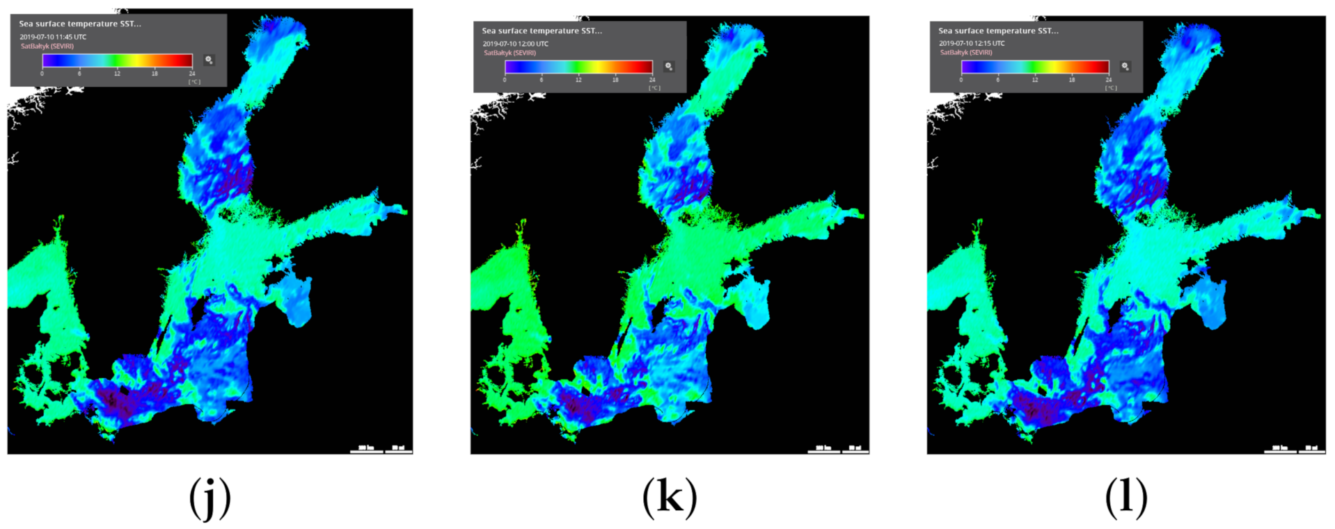
The question in this section is: how can the frequencies computed with moments and invariants be compared and visualized? We would like to superimpose approximate shapes over the surface of the Earth, or more precisely, of the atmosphere over the Baltic Sea. Figure 2 shows the experimental data flow for set A.3—the three following maps with 15-min interval for angular conditions SZA 30–35 degrees. The research data flow goes through the following steps: raw data (satellite image)—calculation of radiation transfer through the atmosphere (cloudiness map 0–1), in Figure 2a–c—determination of the binary cloud mask (0/1), in Figure 2d–f [19]—description of the geometrical elliptical mask (0/1), in Figure 2g–i—derivation of parametric data on their basis Table 2. In addition, SST maps are included for comparison, in Figure 2j–l.

The moments functions that compute the geometrically clouded part of the map are based on fitting a circle, an ellipse, or a rounded shape to the region (the circle fit is computed by fitting the first-order moments, etc., in Mathematica software). To determine the map of moments based on a binary cloud mask, we used the script in MATLAB software. The analytical procedure required fine-tuning of the parameters of the script. A procedure was developed to determine the ellipse parameters for the best fit with a given SatBaltic cloud mask. A useful technique is given in reference [23]. It eliminates clouded pixels when reduced to a binary mask. Since it is statistically difficult to determine which are correct, it is worth looking at a few selected cases, as in Figure 3. The effectiveness of each comparison is determined by the degree of similarity between multiple measurements of the same quantity by different methods: where all case numbers are defined as the sum of: a—the number of cases defined equally as cloudiness by both methods; b—the number of overestimated cases (not defined equally and as cloudiness by one method); c—the number of underestimated cases (not defined equally and as cloudiness by the other method); and d—the number of cases correctly detecting no cloudiness. Ideal detection preserves $H=(ad-bc)/\left(\right(a+c\left)\right(b+d\left)\right)$ at 1; H equals 0 for a statistically random distribution, while negative values classify detection as poor [13]. More detailed instructions for the experimental set-up can be found in Appendix A. The analysis began with unsupervised classifications (successively supplemented with moments) aimed at determining local features for automatically defined data fields. The classification assessed the extent of cloudy areas. In the following part, this study is compared to the supervised solution. There were false positive and false negative areas (underestimated is marked in dark yellow and overestimated marked in white in Figure 2g–i, respectively).

The central moments of the domain D are defined by the integrals [22]

$$M_{mn}:=\underset{D}{\int \int }f(x,y)dxdy,$$

(3)

where $f(x,y)=x^n{y}^m$ is written in the local coordinates, with the origin corresponding to the center of gravity of D. The corresponding discrete form of (3) is given by the sum [22]

$$M_{mn}:=\sum _{P\in D}f\left(P\right),$$

(4)

where $P=(x_i,y_i)$. Following reference [24], we use the invariants of the central moments

$$\begin{array}{c}{I}_1=M_{20}+M_{02},\hfill \\ I_2={(M_{20}-M_{02})}^2+4M_{11}^2,\hfill \\ I_3={(M_{30}-M_{12})}^2+{(3M_{21}-M_{03})}^2,\hfill \\ I_4={(M_{30}-M_{12})}^2+{(M_{21}-M_{03})}^2.\hfill \end{array}$$

(5)

Analogous long formulas take place for the invariants of higher orders [24].

The invariants can be normalized by scaling [24]

$$I_j^{\prime }=-sign\left(I_j\right){log}_{10}(abs\left(I_j\right).$$

(6)

The invariants (5) and (6) are calculated for a selected large cloud displayed in Figure 2 for $I_j^{\prime }$ ($j=1,\dots ,8$). In Figure 4, the cloud is shown in dynamics at the time 10 July 2019–11:45 UTC + 02:00 (blue), 12:00 UTC + 02:00 (pink), and 12:15 UTC + 02:00 (yellow), respectively.

The moments and invariants are calculated by the Formulas (4)–(6) for two sets of data corresponding to Figure 2b,c, at three time points. The values $I_j^{\prime }$ ($j=1,\dots ,8$) are selected in Table 2 for three moments of times. The graphical illustration of the moments in dynamics is displayed in Figure 5. The graphs corresponding to Figure 2b are shown by solid lines, and to Figure 2c by dashed lines. The dashed lines demonstrate the perturbation of the moments calculated for the fixed separate cloud by small clouds surrounding the main cloud or by its fuzzy boundary. One can see that the moments $I_j^{\prime }$ ($j=1,\dots ,8$) changes in time and can compound the principal moment vector which characterizes the considered cloud and its dynamic. The moments $I_j^{\prime }$ ($j=1,2$) changes slowly and can be neglected in the further analysis.

Table 2. Results the calculations of the invariants of the central moments according to Figure 4.

ID	20190710114500		20190710120000		20190710121500
Figure 4	(b)	(c)	(b)	(c)	(b)	(c)
$I_1^{\prime }$	−0.005626	−0.00004	−0.010374	−0.00024	−0.005504	−0.00027
$I_2^{\prime }$	0.314075	0.47134	0.349036	0.566524	0.377664	0.632733
$I_3^{\prime }$	1.310573	1.187512	1.771835	1.536233	1.976419	2.060756
$I_4^{\prime }$	1.488028	2.911716	1.866378	3.104067	2.508078	4.612025
$I_5^{\prime }$	2.122588	3.581997	1.905485	3.603337	2.193086	4.395174
$I_6^{\prime }$	4.106302	6.830714	4.337209	6.961784	5.027498	8.906801
$I_7^{\prime }$	2.783723	4.190248	2.815536	4.404323	3.209285	5.428758
$I_8^{\prime }$	3.933062	6.973255	3.853848	7.029442	4.721769	9.044957

Table 2. Results the calculations of the invariants of the central moments according to Figure 4.

ID	20190710114500		20190710120000		20190710121500
Figure 4	(b)	(c)	(b)	(c)	(b)	(c)
$I_1^{\prime }$	−0.005626	−0.00004	−0.010374	−0.00024	−0.005504	−0.00027
$I_2^{\prime }$	0.314075	0.47134	0.349036	0.566524	0.377664	0.632733
$I_3^{\prime }$	1.310573	1.187512	1.771835	1.536233	1.976419	2.060756
$I_4^{\prime }$	1.488028	2.911716	1.866378	3.104067	2.508078	4.612025
$I_5^{\prime }$	2.122588	3.581997	1.905485	3.603337	2.193086	4.395174
$I_6^{\prime }$	4.106302	6.830714	4.337209	6.961784	5.027498	8.906801
$I_7^{\prime }$	2.783723	4.190248	2.815536	4.404323	3.209285	5.428758
$I_8^{\prime }$	3.933062	6.973255	3.853848	7.029442	4.721769	9.044957

Let us compare the results of effective detection obtained with the four methods:

1. using the conventional technique, from values of radiation transmission ranging from 0 to 1 (at this stage the notation 0.5 means a single pixel half covered by completely opaque clouds or completely covered by semi-transparent clouds [14]) (see references [13,15,16,25]) by linear approximation [14] to 0/1 binary mask (0 if clear/1 if cloudy);

2. the conventional technique supplemented with the method of moments with invariants (0/1 binary mask, 0 if clear/1 if cloudy);

3. the Otsu technique supplemented with the method of moments with invariants [26] (0/1 binary mask, 0 if clear/1 if cloudy);

4. in a supervised manner, with the subjective participation of the observer (0/1 binary mask, 0 if clear/1 if cloudy).

Cloud detection based on selected maps from 9 December 2019 was performed according to methods 1 to 4; the results are shown in Figure 3. Data from 06:00 UTC + 01:00 are presented in the left column (set A.1—the brighter areas correspond to low temperatures) and from 12:00 UTC + 01:00 in the right column (set A.2—the brighter areas correspond to high reflectivity). In the Baltic Sea area, the cloud cover was determined with the conventional method according to the SatBaltic algorithm [13] (method 1) (see Figure 3a,b). The maps were then subjected to a masking operation using the method of moments (method 2); the results are shown in Figure 3c,d. The second order method of moments provides for cloud masking using ellipses; hence, in Figure 3, transparent yellow ellipses appear on the masks. The next pair, Figure 3e,f, represents the results of the statistical work of the Otsu technique with moments added (method 3). The last pair, Figure 3g,h, is the result of the work of a subjective observer. As explained earlier, in the figures, we observe both underestimation (visible light grey fragments) and overestimation of cloudiness (ellipse superimposed on dark grey sea fragments not covered by clouds). The coast/land fragments in the outline of the ellipses are not included.

3.1. Comparative Analysis of Cloud Detection according to Methods 1 and 3

The results of cloud detection in the Baltic Sea area determined according to methods 1 and 3 were compared. In Figure 6a,b, we see a comparison of histograms for the initial map (orange color): after applying the cloud mask according to the conventional SatBaltic algorithm (blue color), and after completing using the method of moments (grey color). The preliminary results show satisfactory results for the application of the method of moments in cloud estimation. The analysis shows that the combination of methods can have a positive impact on the detection, effectively eliminating cloud “noise” initially classified as sea. The cloud cover of the Baltic Sea basin determined according to methods 1 and 3 at 06:00 UTC+01:00 (set A.1) was 43% and 47%, respectively, and, at 12:00 UTC+01:00 (set A.2), it was 39% and 38%, respectively (see Figure 6 and Appendix B). That is, for the map (Figure 6a), the method of moments relative to the conventional method leads to an overestimation of the clouded area by 4%, and, for the reflectance map (Figure 6b), it underestimates it by 1%. Significant differences between the cloud detection paths occurred for intensities in the interval [0.00, 0.30]; pixels in this interval were mostly found in the parts of the satellite image showing sea. For set A.1, the method of moments yielded a cloudiness result that was 7% higher than the conventional methods; for set A.2, the result was 2% lower for the method of moments. For pixel intensities in the range [0.60, 0.75] (pixels from this range were mostly present in the cloud parts of the satellite image), the method of moments yielded cloudiness results 3% higher for set A.1, and 5% higher for set A.2. These results were determined after removing land areas from the moments mask and partly mixing with the measurement uncertainty limit.

3.2. Comparative Analysis of Cloud Detection Results for Methods 1–4

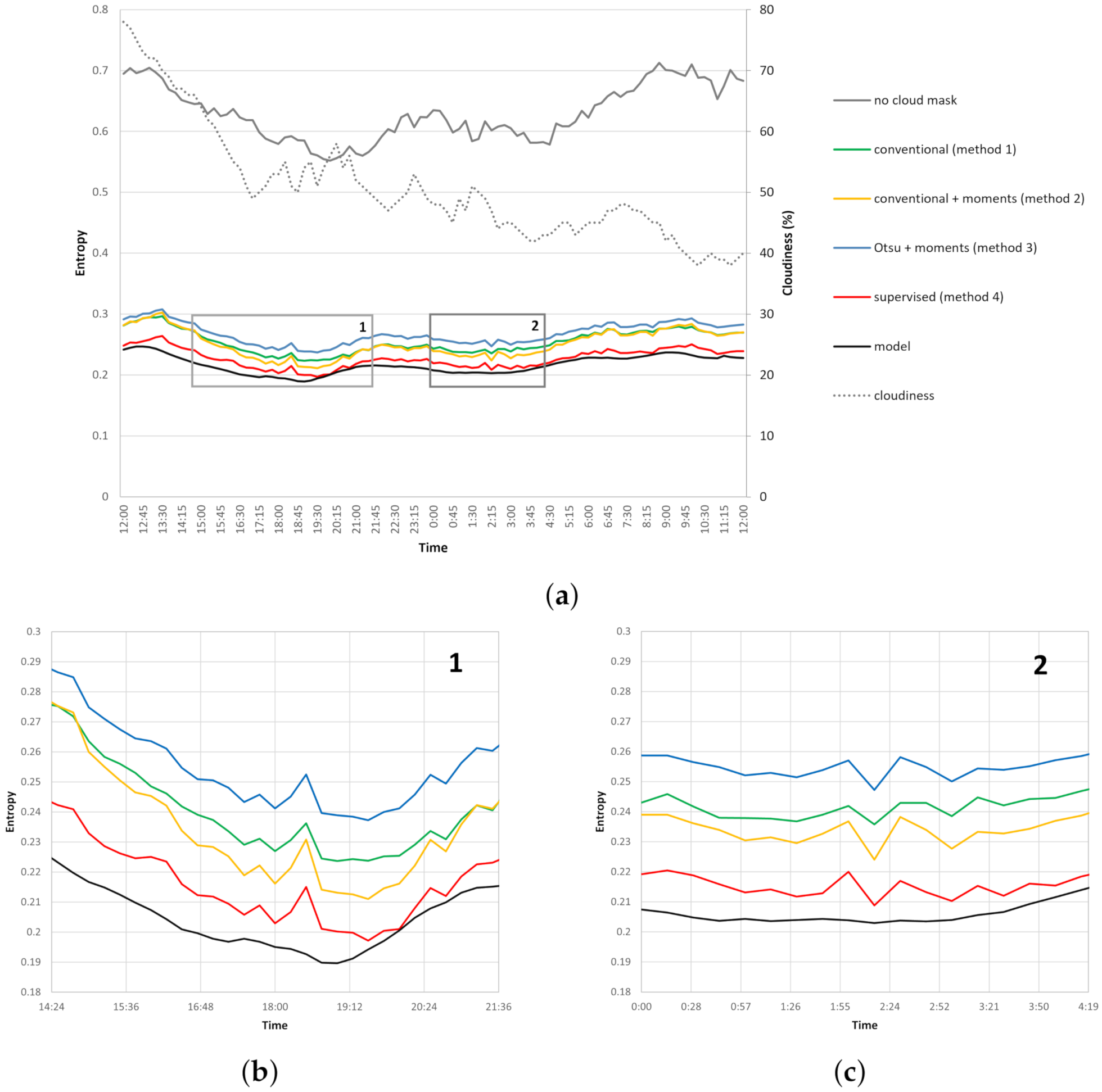
The effectiveness of various cloud detection methods is carried out on the basis of a comparison of the entropy calculation results for the “residuals” of the output image after the cloud masking. According to the research hypothesis, a more adequate method is the one when the result of the calculated entropy is the closest to the entropy of the cloudless model map (black line); see Figure 7. The study is conducted on the basis of data set B (

Table 3. SEVIRI data sets used in further research.

ID	Source File	Date	Time	Remark
A.1	MSG4-SEVI-MSG15-0100-NA-20191209060000	9 December 2019	06:00 UTC + 01:00	Figure 3a
A.2	MSG4-SEVI-MSG15-0100-NA-20191209120000	9 December 2019	12:00 UTC + 01:00	Figure 3e
A.3	MSG4-SEVI-MSG15-0100-NA-20190710114500–	10 July 2019	11:45–	Figure 2a
	MSG4-SEVI-MSG15-0100-NA-20190710121500		12:15 UTC + 02:00	Figure 2b
				Figure 2c
B	MSG4-SEVI-MSG15-0100-NA-20191208120000–	8 December 2019–	12:00–	Figure 7
	MSG4-SEVI-MSG15-0100-NA-20191209120000	9 December 2019	12:00 UTC + 01:00
C	MSG4-SEVI-MSG15-0100-NA-202010	December/2020		Figure 8

), being a 24-h sequence of satellite images from 8 December 2019 12:00 to 9 December 2019 12:00 UTC + 01: 00, taken every 15 min.

By analyzing the entropy diagrams presented in Figure 7, we concluded that, according to this parameter, the use of the alternative method based on moments (method 3), leads to a greater discrepancy of results compared to those obtained by the observer. Methods 1 and 2 yield similar results over the whole observation interval. Let us pay particular attention to the time intervals from 16:00 to 21:00 UTC + 01:00 (Figure 7b) and from 0:00 to 5:00 UTC+01:00 (Figure 7c), in which the predominance of method 2 in cloud detection is observed (based on a measure of entropy). The comparison of these results with the cloud cover curve leads to the research hypothesis that it is particularly appropriate to use method 2 in periods of forecasted high cloud cover variability. In these two time periods, the changes of cloudiness took place every 15 min at an amplitude of approximately 5%.

In more complex situations (Figure 8), this comparison shows that the moments method can effectively support unsupervised detection (for a relatively large data set, this depends on some elimination of clouds that do not contrast with the sea). The Baltic pixels remaining after masking determine the entropy described by Figure 7a. Additionally, the dashed line in Figure 7a shows the cloudiness of the Baltic Sea. The extent of the binary mask depends on the method, the product of the statistical moment map, or the opinion of the subjective observer. The last one takes place in a supervised procedure, allowing areas difficult to detect by automatic methods to be completed. This has been demonstrated by analyzing less turbid areas, while keeping entropy at its lowest level. At this stage, it is difficult to say that the alternative method of moments (method 3) is superior to the conventional solutions (method 1), but, due to the high correlation of the solutions, we can consider it an interesting addition. The final product could be a conventional cloud mask with added moment shapes (method 2), whose aim is not to compete with nor replace existing solutions but to complement them. Specifically, Figure 7a specifies two periods (1 and 2, in Figure 7b,c), where a combination of solutions improves the results. It should be noted that these are spectrally and spatially well-defined objects. To demonstrate that the method indeed has the potential to parameterize cloud signaling, a 1-month satellite image sequence was used (Figure 8).

Figure 7 and Figure 8 shows the entropy value of the SatBaltic maps after masking in an automatic and supervised manner. The quantitative evaluation of the method consists of determining the entropy difference between the conventional and assisted moments and the supervised solution.

The moments method allowed the entropy to be decreased by a 3%, while eliminating a underestimated area 5%. It is clear that underestimated sea areas occur, but the decreased estimation of entropy becomes high enough not to be ignored in the overall budget. In general, as can be seen in Figure 8, cloud cover can be estimated with moments, but significant uncertainties arise. Uncertainty estimation is not the goal at this stage; the goal is to effectively demonstrate the potential for improving conventional analysis using the moments method.

On the other hand, for poorly-defined cloud formations, overestimation may result from the assumptions of the method itself. Such formations cover rather large areas, so they extend to the semi-transparent regions (e.g., blurred cloud edges). As shown above, the moments method accomplishes this task by extending the cloudiness estimate to areas that are considered cloud-free by operational cloudiness detection systems. Further references to other operational cloud detection systems can be found in reference [13]. Clouds are also characterized by multicoherent regions (e.g., an ellipse within an ellipse) due to the great diversity in their structures. Each ellipse contains a set of statistical parameters that we use for further processing, for example, providing data for machine learning. A set of clouds in the atmosphere can be modeled as a set of inclusions embedded in a bulk medium with physical properties, such as density, thermal and electrical conductivity, etc. Due to the different physical properties of clouds and the surrounding air, interactions between clouds are possible. In this model, interactions of physical fields, not mechanical collisions, are captured. With the help of this method, we naturally arrive at the consideration of cloud sets as a two-phase medium. This theory is outlined in the following section.

3.3. Structural Sums

The theory of two-phase media is based on the field interactions of inclusions dispersed in a bulk medium. These interactions are described by various partial differential equations. In reference [21], it was shown that a sufficiently large class of such phenomena can be described by the structural approximations associated with a graph. It was proven in references [9,10] that expressions for the macroscopic physical properties can be decomposed into a linear combination of the structural sums. The set of structural sums associated with any geometric object is infinite, and one usually takes its finite subset. To be consistent with references [9,10], the following scaling is used. The coordinates of the square in Figure 6 are reduced by a linear transformation to the unit square $(-0.5,0.5)\times (-0.5,0.5)$. The corresponding ellipse centers are written in terms of the complex coordinates $a_k=x_k+i{y}_k$, where $(x_k,y_k)$ denotes the Cartesian coordinates of the centers, and i the imaginary units. Let $A_k$ and $B_k$ be the semi-axes of the kth ellipse. Its area is

$$s_k=\pi A_k{B}_k.$$

(7)

Let $E_p\left(z\right)$ denote the Eisenstein function of order p [9,21]. These functions are related to the classic Weierstrass elliptic functions by simple formulas and are usually implemented in standard packages. The low-order structural sums are introduced as below. The clouds of significant area are taken into account in the example in A.2 ($N=20$). Introduce the area fraction of clouds in the normalized unit cell

$$f=\sum _{k=1}^N{s}_k.$$

(8)

Introduce the low-order structural sums following references [9,21] and using another scaling in concentration f:

$$e_2=\frac{1}{f^2{N}^2}\sum _{k=1}^N\sum _{m=1}^N{s}_k{s}_m{E}_2(a_k-a_m),$$

(9)

and

$$e_{pp}=\frac{{(-1)}^p}{f^{2p}{N}^{p+1}}\sum _{k=1}^N|\sum _{m=1}^N{s}_k{s}_m{E}_p(a_k-a_m){|}^2,p=2,3,4.$$

(10)

Here, $\left|z\right|$ denotes the modulus of the complex number z. It is assumed that $E_2\left(0\right):=\pi$ by definition when $a_k=a_m$ for shortness in the sums (9) and (10). For the cases in question, we have:

$$(e_2,e_{22},e_{33},e_{44})=(0.00929-0.00278i,0.0123,-0.11,31.86),$$

(11)

and, in A.1, it is:

$$(e_2,e_{22},e_{33},e_{44})=(0.00262-0.037i,0.247,-579.4,1.47·{10}^6).$$

(12)

These are characteristic vectors of this set of clouds. The monodispersed structural sums were considered in references [9,10]. For instance, $e_2^{mono}$ is defined by (9) with $f=1$ and $s_k=s_m=1$. The values $e_2^{mono}=3.05+1.16i$ and $e_2^{mono}=0.0478-0.6798i$ for sets A.1 and A.2, respectively, characterize the macroscopic isotropy of the corresponding cloud phase. For an ideally isotropic set, we have $e_2^{mono}=\pi$. It can be seen thatm for different vectors, (11) and (12), calculated for sets A.1 and A.2, we get different results. This means that the first group of clouds is more isotropic than the second. In this simple way, the information calculated graphically shows the extent of anisotropy of the cloud cluster. The cloud moments, as well as the cloud clusters, are different; this applies to both groups and individual moments with elliptical shapes (

Table 4. The values of moments for the examples discussed.

ID	${\mathit{M}}_{11}$	${\mathit{M}}_{20}$	${\mathit{M}}_{02}$	$[{\mathit{I}}_1,{\mathit{I}}_2]$	$[{\mathit{I}}_1^{\prime },{\mathit{I}}_2^{\prime }]$
A.1	−0.1346	0.7434	0.5993	[1.3427, 0.0933]	[−0.1280, 1.0302]
A.2	−0.2919	1.0850	0.5365	[1.6215, 0.6416]	[−0.2099, 0.1927]

).

The final features of the satellite image (given as input data) are the values $[{\phi }_1,{\phi }_2]$. These functions are used to recognize clouds from an satellite image and can be used to recreate an mask of clouds. The advantage is that the mask is reduced to a few mathematical functions related to the cloud’s features. The structural sums $e_{22}$, $e_{33}$, and $e_{44}$ include the higher orders of correlation functions and characterize the “total” shape of the set of clouds. It follows from general theory [9,10] that an infinite set of structural sums completely describe the set. Therefore, its truncation (11) approximates the structure in question.

4. Discussion

The cloud detection process requires many different methods, such as dynamic thresholding, surface analysis, etc. Each of the above-mentioned methods has its own strengths and weaknesses [16]. New solutions, such as machine learning [5], are often unstable and require some parameterization. The main goal of this research is to obtain a data set of parameters of the geometrical structures (i.e., values of invariant moments) that models real satellite images. The obtained data set will be used in our further research to make a prognosis of the cloudiness changes. The method of moments can be used to complement satellite-based solutions. Its main advantage is that it supports the detection of objects with regular shapes on a local scale by overestimating regions that are conventionally difficult to detect but physically justified (e.g., blurred cloud edges).

There may be some concerns about the representation of a complex cloud structures with compact shapes, such as ellipses. However, clouds as atmospheric objects have a natural tendency to form compact structures due to the accompanying physical phenomena, including electrostatic interactions. Therefore, the method works well for predicting dynamics events. A valuable advantage of the method may be the obtained parameters defining geometric structures, which can be used in further research. The mask of the sea is a certain obstacle, and, in the next stage, a procedure will be developed, allowing for the extension of the research area with adjacent pieces of land. However, it is important to understand the important differences in the detection of clouds over water and over land. In more complex situations, it can effectively support oceanographic analyses (e.g., for a large data set that does not contrast with the sea, even at the expense of possible overestimation).

5. Conclusions

Improving the quality of cloud analysis is of great importance in various branches of science, from oceanology to climatology. In order to successfully complement the detection of clouds on a regional and local scale, more attention should be paid to the analysis of objects visible on the background of the sea. One of the way to achieve this goal is to introduce additional geometric parameters at the level of the raw digitized satellite image, before applying the image analysis methods. Conventional methods for eliminating noise to obtain a homogeneous map may lead to a loss of important satellite image features, thus lowering the recognition accuracy. The innovative method of cloud detection presented in the article is based on the theory of unchanging moments and structural sums. This allows the parameters of the problem to be optimized. In this paper, the theory of moments and structural approximation are used to consider a set of clouds as a two-dimensional geometric object. The corresponding shape moment vector is assigned to a separate cloud. Moreover, a cloud set is investigated as a multi-connected domain by structural approximation in order to describe the interactions between separate clouds within the set. This method consists of combining the basic features of an satellite image on the same scale in different directions, according to the rule of unchanging moments, in order to detect an object for identification. The experimental results show that the proposed method is effective and parameterizes the detection of satellite image features. In the next step, the set of relations (11) and (12) will be used in the application of machine learning and for classifying cloudiness based on structural sums and the analysis of feature vectors $(e_2,e_{22},e_{33},e_{44})$ and $\left\{M_{mn}\right\}$.