Article

Cotton Classification Method at the County Scale Based on Multi-Features and Random Forest Feature Selection Algorithm and Classifier

1
School of Information Engineering, Tarim University, Alaer 843300, China
2
Southern Xinjiang Research Center for Information Technology in Agriculture, Tarim University, Alaer 843300, China
3
College of Information and Electrical Engineering, China Agricultural University, Beijing 100083, China
*
Author to whom correspondence should be addressed.
Remote Sens. 2022, 14(4), 829; https://doi.org/10.3390/rs14040829
Submission received: 10 December 2021 / Revised: 22 January 2022 / Accepted: 7 February 2022 / Published: 10 February 2022

Abstract

:
Accurate cotton maps are crucial for monitoring cotton growth and precision management. The paper proposed a county-scale cotton mapping method by using random forest (RF) feature selection algorithm and classifier based on selecting multi-features, including spectral, vegetation indices, and texture features. The contribution of texture features to cotton classification accuracy was also explored in addition to spectral features and vegetation index. In addition, the optimal classification time, feature importance, and the best classifier on the cotton extraction accuracy were evaluated. The results showed that the texture feature named the gray level co-occurrence matrix (GLCM) is effective for improving classification accuracy, ranking second in contribution among all studied spectral, VI, and texture features. Among the three classifiers, the RF showed higher accuracy and better stability than support vector machines (SVM) and artificial neural networks (ANN). The average overall accuracy (OA) of the classification combining multiple features was 93.36%, 7.33% higher than the average OA of the single-time spectrum, and 2.05% higher than the average OA of the multi-time spectrum. The classification accuracy after feature selection by RF can still reach 92.12%, showing high accuracy and efficiency. Combining multiple features and random forest methods may be a promising county-scale cotton classification method.

1. Introduction

Cotton is a significant economic crop in China, covering approximately 3,168,910 hectares in 2020 [1], one of the significant cotton lint-producing countries with 5,910,500 tons, accounting for approximately 24% of global cotton production (FAO, 2020). Accurate statistics for a large area of cotton are prerequisites for yield estimation [2,3,4], agricultural production management [5], and various types of research [6,7]. As a large-scale, multi-temporal monitoring method, remote sensing technology has been increasingly applied in many aspects in recent years, such as resource management [8], agricultural monitoring [9], environmental monitoring [10], mineral exploration [11], etc. According to the information provided by the National Bureau of Statistics of China, the annual cotton planting area in Xinjiang is obtained through a combination of remote sensing and sampling surveys, but county-scale and detailed cotton planting areas and maps are not provided. For production managers and scientific researchers, it is necessary to provide a convenient way to obtain county or field-scale cotton distribution mapping. Therefore, it is of great practical significance to study county-scale cotton remote sensing classification methods for field management, precision agriculture, and government decision making.
So far, many countries have been studied using satellite observations for land-cover classification and crop yield forecasting (Table 1), for example, Brazil [12], Uzbekistan [13,14], China [15,16,17], and Mali [18]. The spectral, temporal, and spatial characteristics are the primary theoretical basis for remote sensing image classification [19]. The spatial resolution of satellite images used in these studies ranges from hundreds of meters to less than 1 m. Satellite images with low spatial resolution usually cover a larger area, which is beneficial for large-scale agricultural monitoring. By improving the time resolution, complex classification can be achieved with the help of phenological rules [20,21]. For example, Huang et al. [22] developed a crop model and data assimilation framework that assimilated leaf area index (LAI) derived from time-series Landsat TM and MODIS data to estimate regional wheat yield predictions. Xun et al. [23] explored the feasibility of combining time-series enhanced vegetation index (EVI) computed from MODIS satellite data with a fused representation-based classification (FRC) algorithm to identify cotton pixels and map cotton acreage. However, due to the mixed pixels of low- and medium-resolution (hundreds of meters) remote sensing images, it is difficult to obtain accurate classification results. Increasing the spatial resolution of the image can solve mixed pixels; for example, Zhang et al. [16] used WorldView-2 images to classify crops in smallholder agricultural areas accurately. However, due to the cost constraints of image acquisition, storage, and calculation, very high-resolution (less than 10 m) images are not suitable for county-level monitoring. More researchers choose medium and high resolution (tens of meters) images, such as Landsat and Sentinel, for agricultural observation research.
In addition to increasing the spatial and temporal resolution, methods to improve the classification accuracy mainly include classifier selection and parameter tuning [24], integrating multi-source remote sensing information [25,26], etc. In recent years, some machine learning algorithms, such as ANNs [27,28], decision trees (DTs) [29,30], SVMs [31], etc., have been widely used in remote sensing image classification. In addition, deep learning has also brought new possibilities in many remote sensing research fields, such as image optimization [32,33], object detection, and classification [2,34]. However, various machine learning classifiers often show different performances in different research objects [35]. For example, Edwin Raczko and Bogdan Zagajewski compared SVM, RF, and ANN algorithms in tree species classification and believed that RF achieved higher overall classification accuracy than SVM [36]. However, Phan Thanh Noi et al.’s study on the classification of land cover types showed that SVM produces higher overall accuracy than RF [37]. In view that we have not retrieved a comparative study of cotton classification methods in the current literature search, it is necessary to evaluate the classifier’s performance for this task.
To further improve the classification accuracy, the various features of the image, such as spectral features, temporal features, texture features, digital elevation models (DEM), and other features, can be added to the classifier [38]. Al-Shammari et al. [39] added the magnitude and phase features of the NDVI time series to the classification features, which improved the cotton extraction accuracy. In the existing classification research, texture features are often used in object-based image analysis (OBIA) [16,40,41], but they are rarely used in pixel-based image analysis. Nevertheless, the research of Chen et al. [42] showed that texture features play a role in promoting image fusion and classification in pixel-based research. Zhang et al. [43] used the spectral and texture features obtained by Landsat 5 to classify complex areas using an RF classifier, showing that the method has the potential to improve land cover classification accuracy. In recent studies on cotton classification research, the texture was added to the classification of Tiangong-2 images to improve the extraction accuracy of cotton [44]. You et al. [45] used optimized features from spectral, temporal, and texture characteristics of the land surface to create a crop map of Northeast China, and the estimates agreed well with the statistical data for most of the municipalities.
Involving too many features in classification may cause information redundancy, which will reduce the classification efficiency or even classification accuracy [46]. Feature engineering is essential preparatory work for machine learning. Applying a reasonable feature selection approach is critical to effectively reduce feature redundancy and improve the efficiency and accuracy of classification [47]. Feature selection methods commonly include filter, wrapper, and embedded methods [48,49]. Filter methods directly delete features from the original feature set and quickly select important features, but it is challenging to reduce redundancy for multiple features with high correlation. Wrapper and embedded algorithms select features concurrently with the learning process and generally lead to better results than filter methods. Some studies have confirmed that machine learning algorithms, such as RF, SVM, etc., can easily and efficiently achieve feature scoring and selection [50], but the required features must be selected according to some rules.
In order to achieve county-scale cotton classification, this paper explored and evaluated a cotton mapping method based on multi-features, random forest (RF) feature selection algorithm and classifier to improve accuracy and efficiency. The main objectives were to (1) Explore the contribution of texture features to cotton classification accuracy in addition to spectral features and vegetation index. (2) Attempt to use RF feature screening methods to improve classification efficiency. (3) Evaluate the effects of image acquisition time, feature importance, and the best classifier on the cotton extraction accuracy.

2. Materials

2.1. Study Region

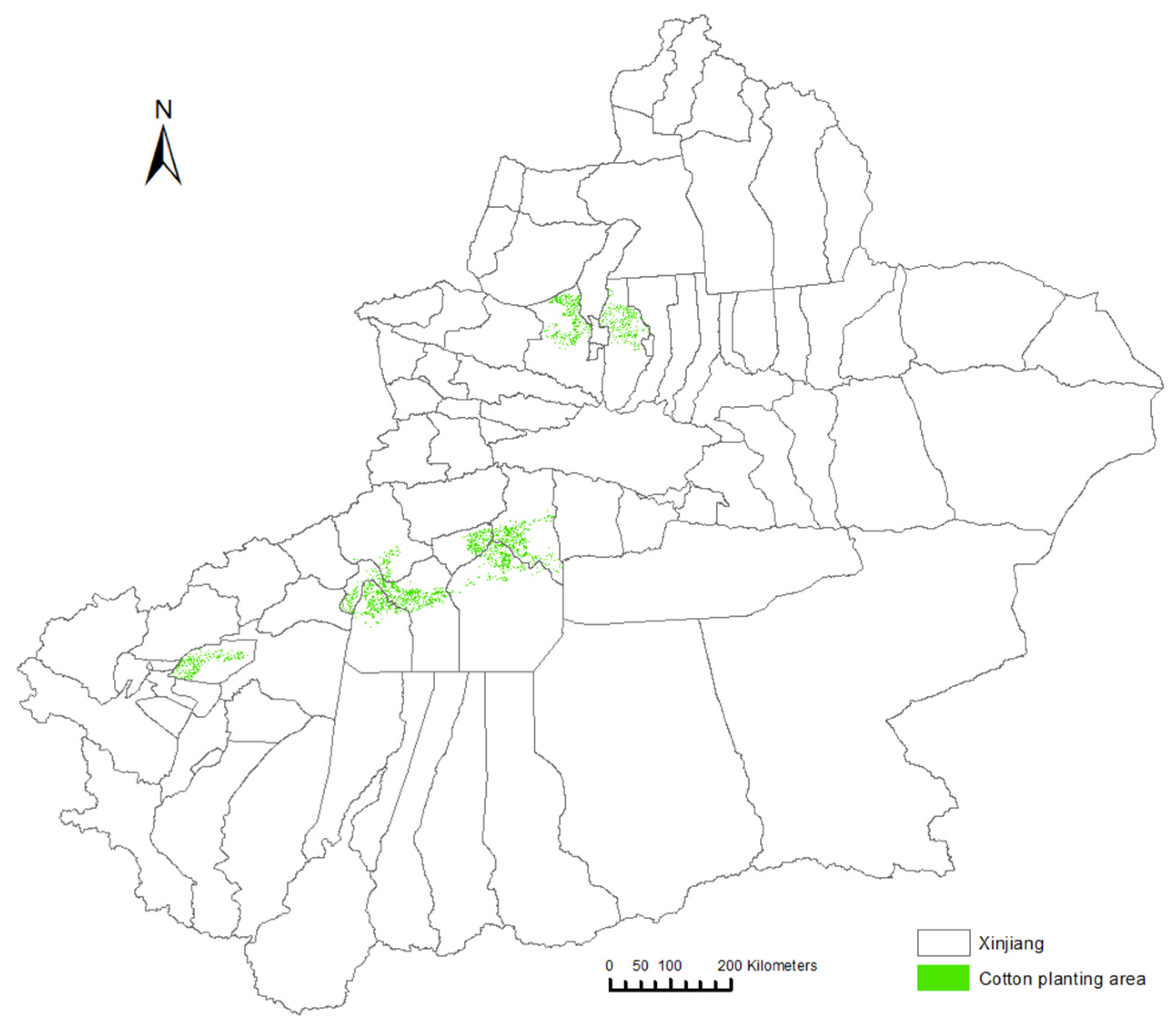
This study selected ten counties with high cotton production in Xinjiang, China, to carry out experiments. The study area is located in the north and south of the Tianshan Mountains, a temperate continental climate zone. Due to its unique geographical location, the region has little precipitation and a dry climate, but it has sufficient sunshine and abundant river water resources. The main field surveys were carried out in the Aksu area, and visual interpretation was carried out in other counties based on the spectral characteristics of various ground features. Cotton is an important crop in this region. In 2017, the cotton planting area in the selected area was approximately 930,000 hectares, accounting for 42% of Xinjiang. Figure 1 shows the distribution of cotton planting areas in various counties, of which six counties have cotton planting areas over 100,000 hectares. In this study, counties with a large cotton planting area were selected as the study area, as well as some counties with a small cotton planting area. Therefore, the selection of the study area makes the experimental results more convincing.

2.2. Data and Preprocessing

2.2.1. Remote Sensing Image Data

In this study, the remote sensing data came from USGS EarthExplorer (https://earthexplorer.usgs.gov/), and the Landsat 8 L1T data with less cloud cover during the growth period of cotton was selected. As Landsat 8 L1T data has been geometrically corrected, only radiometric calibration and atmospheric correction were completed. The vector boundary data of the county was used to cut and mosaic the corrected image to obtain the image within each county. Since images at a specific time may be affected by clouds, when images at the same time within the county area cannot be obtained, images at adjacent times were used for mosaicking to obtain images at the county area. Finally, the time distribution of the images available in each county is shown in Figure 2. Among them, the abscissa is the number of days on the observation date in 2017.

2.2.2. Ground Sample Data

Field surveys were mainly conducted in the Alar reclamation area, using GPS to locate and mark the types of ground targets. The collected samples included 202 cotton samples, 142 fruit tree samples, 84 rice samples, 45 other crop samples, 74 bare land samples, and 47 water samples. Each sample is a small area containing multiple pixels. Based on the collected sample data, the spectral characteristics of various ground objects could be summarized, and reasonable visual interpretation could be performed on remote sensing images in other regions. Non-repetitive sampling was performed for each region, and these samples were divided into training samples and verification samples at a ratio of 3:1 to construct a sample dataset.
Table 2 shows the planting area of main crops in each unit in the study region. The main crops in the study area included cotton and fruit trees (such as jujube, apples, etc.), while other annual crops such as wheat and maize, which account for a smaller proportion, were classified as “other crops”. Rice was classified into a single category because its spectral characteristics were similar to water in the early growth period. In addition, different types of non-crop classes (forests, water, bare land, etc.) were registered to obtain non-crop classification data. The actual sown area of various crops refers to the Xinjiang statistical yearbook and Xinjiang Production and Construction Corps statistical yearbook.

3. Methods

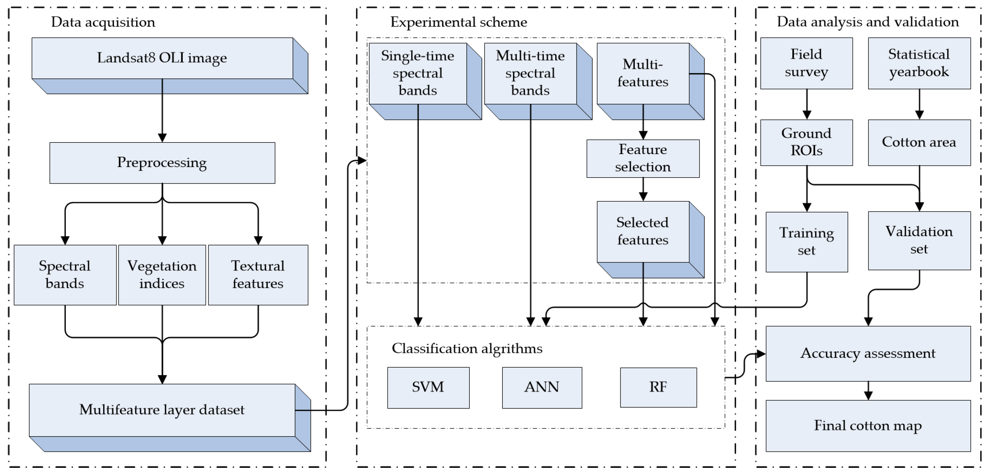
Figure 3 provides the technical research route of this article. This study used Landsat 8 OLI images; the spectral band, vegetation index, and texture features were extracted to construct the feature space, all features of the feature space were sorted and selected using a random forest (RF) algorithm. Then, three relatively mature machine learning algorithms were used to classify the original spectral images and the composite feature images and identify and extract the cotton planting area. According to the different features added to the classifier, the experiment was divided into four groups to evaluate various features on the classification results. The same experimental scheme was used for classification in multiple counties to compare classification results and evaluate the adaptability of classification methods in different regions.

3.1. Feature Extraction

3.1.1. Spectral Bands

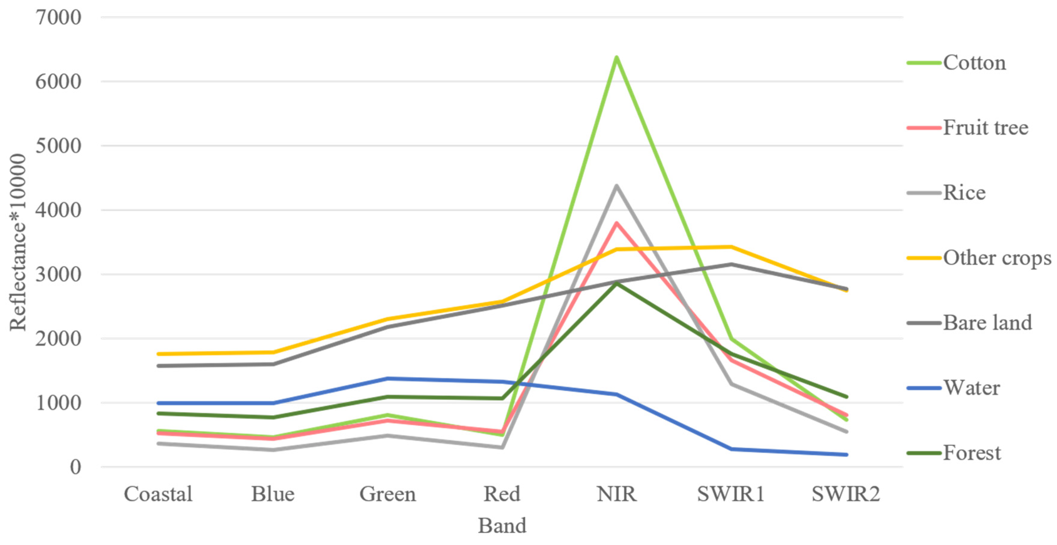
Multi-spectral remote sensing images record the reflectivity of multiple bands in the electromagnetic spectrum. Different types of ground objects have different reflectivities of electromagnetic waves in each band. Therefore, the object can be distinguished from other categories based on its spectral reflectance characteristics. Referring to the spectral reflectance curves of various ground objects in July (Figure 4), it was found that cotton reached a very high peak in the NIR band, which was significantly different from other ground objects. This is because green plants have strong absorption in the red (R) band and strong reflection in the NIR band. Some studies suggest that red edge and NIR bands are important in crop research [51,52]. However, it is worth mentioning that the value of the spectral reflectance curve here was the average value obtained in many sample points. In the image, the actual reflectance value of each sample point fluctuated up and down. In a particular band, the range of reflectance values for different crops overlapped. Therefore, even if the spectral reflectance curves of various ground objects had apparent differences, it was not feasible to use this feature to classify them. Other bands with apparent differences in spectral reflectance curves are the R and SWIR1 bands. The reflectance data of these three bands were extracted to construct a spectral feature library.

3.1.2. Vegetation Indices

An appropriate vegetation index can be used for various applications in scientific research, such as plant classification, growth monitoring, and studying plant diseases and insect pests. The vegetation index (VI) is obtained by calculating the different spectral bands of remote sensing images based on the difference in reflectance of vegetation between different spectral bands [19]. Because vegetation has strong absorption in the R band and high reflectivity in the NIR band, the difference and ratio of the NIR and R bands are often used to distinguish vegetation from non-vegetation. Many vegetation indices are calculated based on the R and NIR bands to reflect the growth of vegetation, such as the differential vegetation index (DVI), ratio vegetation index (RVI), normalized vegetation index (NDVI), etc. Many scholars and experts have proposed various vegetation indices suitable for different scenarios according to particular application scenarios. For example, when the vegetation coverage in the study area is high, a vegetation index such as NDVI tends to be saturated, making classification difficult. The enhanced vegetation index (EVI) adds blue bands to enhance the vegetation signal and correct the influence of soil background and aerosol scattering, which can solve the saturation phenomenon and is suitable for terrains with lush vegetation. In areas with low vegetation coverage, the vegetation index is greatly affected by the soil background. The soil-adjusted vegetation index (SAVI) can adjust the parameters according to the vegetation coverage to reduce the impact of the soil background. In this study, a total of 5 vegetation indices were selected, including DVI, RVI, NDVI, SAVI, and EVI. The calculation formula is shown in Table 3.

3.1.3. Texture Features

Texture features can be used to distinguish ground objects with similar spectral features [53]. Image texture is a description of image homogeneity, representing the spatial arrangement and change frequency of continuous pixels in the local neighborhood of the image [54]. The texture feature is not based on the feature of a pixel, it is calculated by the distribution rule between the neighborhood of the image pixel and the pixel, so it has a strong resistance to the noise of a single pixel. Within the scope of the field, the type of crop is generally single and has good homogeneity, so adding texture features is helpful to distinguish the field from other categories. Calculating texture features by generating a gray level co-occurrence matrix (GLCM) is a representative statistical method generated by calculating the pixel pairs’ frequency with specific values and specific spatial relationships in the image [42]. GLCM can be understood as the number distribution table of the pairwise combinations of all different element values in the original matrix, the order of which is equal to the gray level of the original matrix. First, we determined the spatial direction and spacing of the pixel pairs to specify the traversal rules and then traversed the original gray-scale image to find the number of pixel pairs in a specific relationship. The element value of the generated gray-level co-occurrence matrix is the number of pixel pairs. Calculating statistical metrics from the generated GLCM can express the texture characteristics of the original image. The second-order probability statistical filtering method (co-occurrence measures) displays the image by calculating the frequency of specific pixels in two windows in a gray image. The relationship between the element and its specific neighborhood is GLCM. When calculating, it is necessary to determine the size of the window, the direction, and the distance of translation to determine the thickness of the texture feature. Since remote sensing images are composed of multiple spectral bands, the texture features were obtained by statistical calculation of a one-dimensional image. Therefore, the principal component analysis (PCA) was performed on multiple spectral bands of the remote sensing image, and the first principal component was taken to calculate the texture feature. In our experiments, the first principal component often contained more than 80% of the information in the multi-spectral image, so it can be approximately considered that the texture features extracted by the first principal component reflect the shape information of the multi-spectral image. The texture feature calculation formulas [55] used in this research are shown in Table 4, where:
P i , j = V i , j i , j = 0 N 1 V i , j
i is the row number, and j is the column number. V is the value in the cell i,j of the image window. P i , j is the probability value recorded for the cell i,j.

3.2. Classification Based on Random Forests

In remote sensing image classification research, various machine learning classifiers often show different performances in different studies due to research objects and methods [36]. Noi et al. [37] calculated the literature from 2007 to 2017 and found that support vector machine (SVM), random forest (RF), maximum likelihood (MLC), and artificial neural network (ANN) are the four most commonly used classifiers. In this study, we chose three classifiers for comparison, i.e., SVM, RF, and ANN, and emphasized the essential issues when using these classifiers. The SVM classification in this study used the RBF kernel, and the penalty parameter was set to 0.7. For ANN, in terms of parameter settings, we chose the number of hidden layers to be two and adjusted the training rate to stabilize the training error below 0.3. Random forest methods usually do not require complex parameter modulation processes. The number of trees is the most critical parameter, which was set to 100 in this study.

3.2.1. RF Description

RF is a commonly used algorithm in feature importance measurement. It can not only realize feature selection, but also has good accuracy and robustness of classification [56]. Due to its fast-training speed, high precision, and no need for complex parameter adjustments, the RF model has apparent advantages in feature selection [57]. The RF [58] algorithm implementation process is as follows:
Step 1: A random forest is a classifier consisting of a collection of tree structured classifiers { h ( X , Θ k ) ,   k = 1 , 2 , } where the { Θ k } are independent identically distributed random vectors, and each tree casts a unit vote for the most popular class at input x.
Step 2: Given an ensemble of classifiers h 1 ( x ) ,   h 2 ( x ) ,   ,   h K ( x ) , with the training set drawn at random from the distribution of the random vector Y , X , define the margin function m g ( X , Y ) , see Formula (2).
m g ( X , Y ) = a v k I ( h k ( X ) = Y ) m a x j Y a v k I ( h k ( X ) = j )
Step 3: As the number of trees increases, for almost surely all sequences, P E * converges to Formulas (3) and (4).
P X , Y ( P Θ ( h ( X , Θ ) = Y ) m a x j Y P Θ ( h ( X , Θ ) = j ) < 0 )
P E * = P X , Y ( m g ( X , Y ) < 0 )
Step 4: The margin function for a random forest is m r ( X , Y ) , see Formula (5).
m r ( X , Y ) = P Θ ( h ( X , Θ ) = Y ) m a x j Y P Θ ( h ( X , Θ ) = j )
The strength of the set of classifiers h ( X , Θ ) is as follows, see Formula (6).
s = E X , Y m r ( X , Y )
Step 5: A more revealing expression for the variance of m r is derived in the following, see Formula (7).
J ^ ( X , Y ) = a r g   m a x j Y P Θ ( h ( X , Θ ) = j )
Therefore, the margin function for a random forest is shown in Formula (8).
m r ( X , Y ) = P Θ ( h ( X , Θ ) = Y ) P Θ ( h ( X , Θ ) = J ^ ( X , Y ) ) = E Θ [ I ( h ( X , Θ ) = Y ) I ( h ( X , Θ ) = J ^ ( X , Y ) ) ]
The raw margin function is shown in Formula (9).
r m g ( Θ , X , Y ) = I ( h ( X , Θ ) = Y ) I ( h ( X , Θ ) = J ^ ( X , Y ) )
An upper bound for the generalization error is given by Formula (10).
P E * ρ ¯ ( 1 s 2 ) s 2
where, ρ ¯ / s 2 is the correlation divided by the square of the strength. In understanding the functioning of random forests, this ratio will be a helpful guide; the smaller it is, the better.

3.2.2. Feature Selection Based on Random Forest (RF)

RF is an embedded method that uses Gini index, or out of bag data (OOB) error rate, to quantitatively evaluate the contribution of each feature in the model training process. This allows the feature importance ranking. According to the ranking, feature bands of high importance are selected for combination, and the combined multi-feature image is obtained for classification.
In this research, scikit-learn was used to implement the RF algorithm and feature importance evaluation. Scikit-learn is a set of python modules for machine learning. In addition, implementing learning algorithms can simply and efficiently accomplish data loading, divide training and validation sets, and conduct data preprocessing. Scikit-learn provides a method based on a Gini index to evaluate the importance of features. The Gini index can quantitatively evaluate the ability of a feature to separate instances from different categories [59]. For each node of the decision tree, assuming that the sample set s contains m categories, the Gini index is defined as [60]:
G i n i ( s ) = i = 1 m p i ( 1 p i ) = 1 i = 1 m p i 2
where, p i is the proportion of observations in the i-th class. At each node of the decision tree, it is necessary to search all features and find a value to distinguish different categories and minimize the Gini impurity. Finally, according to its contribution to reducing Gini impurities, the importance score for each feature is obtained.
The random forest function in scikit-learn has many parameters. Among them, the parameter “n_estimators” has the most significant impact on the classification result, representing the number of trees in the random forest. In the RF algorithm, setting this parameter to 100 can achieve better training results [61]. If the number of samples or features is large, some parameters of the subtree need to be adjusted, such as “max_depth”, “min_samples_split”, etc.

3.3. Accuracy Evaluation

The confusion matrix obtained by the verification samples can be used to obtain parameters such as overall accuracy (OA), Kappa coefficient, producer accuracy (PA), user accuracy (UA), etc. The classification accuracy based on pixels is usually evaluated by OA and the Kappa coefficient [62]. PA and UA are used to evaluate the classification accuracy of a single category of ground objects from the perspective of map producers and users. The difference between PA and UA is the reference data. In pixel-based classification, the reference data for PA is the actual number of pixels in the category. The reference data for UA is the number of pixels divided into that category. However, the evaluation parameters obtained by the confusion matrix depend on the verification samples. Since the verification samples cannot fully cover the study area, neither the misclassification nor the omission can be detected in the unsampled area. Therefore, referring to the actual area of cotton, the relative accuracy of the cotton area (RAC) in the classification result was used as the evaluation index of the classification result. The predicted area of cotton could be calculated by the pixel points of the cotton category in the statistical classification results. The cotton sown area in the Xinjiang Statistical Yearbook was used as the actual area to calculate the relative accuracy of the cotton area. In this study, five parameters, OA, Kappa, PA, UA, and RAC, were counted according to the validation samples of the ROI to evaluate the accuracy of classification results. The formulae are as follows:
O A = i = 1 r x i i N
where i = 1 r x i i represents the number of pixels of all samples correctly classified, and N represents the total number of samples.
K a p p a = P o P e 1 P e
where P o represents the correctly allocated samples (the proportion of cases in agreement), and P e is the hypothetical random agreement.
P A = C c C t
where C c represents the correctly classified samples of a specific class, and C t is the total number of pixels in the category.
U A = C c C r
where C r represents the total number of pixels classified into this category.
R A C = ( 1 | P A C A A C | A A C ) × 100 %
where RAC represents the predicted area of cotton, and AAC represents the true area of cotton.

3.4. Experiments

Various experiments were conducted on ten county-level units to improve the classification accuracy and find suitable methods for extracting the cotton area in different regions. Only agricultural production areas were cropped for image classification for some vast counties, ignoring mountainous areas and deserts. Spectral image, vegetation index, and texture features were combined into a learning database for each area.
  • In terms of feature selection, the RF model was used first to learn the training samples, and the obtained model was used to rank the importance of all features in the learning database. Then, a certain number of features were selected for classification in a stepwise manner. The RAC of the classification results was used as an evaluation index to determine the number of feature bands to be selected.
  • The classification experiment was divided into three groups according to the different bands of the added images: (1) classification based on single-phase spectral images; (2) classification based on multi-phase spectral images; (3) classification based on the learning feature library of multi-time spectral images, vegetation index, and texture features; and (4) classification based on multi-feature images after feature selection on the learning database.

4. Results and Discussion

4.1. Feature Selection Based on Random Forest Algorithm

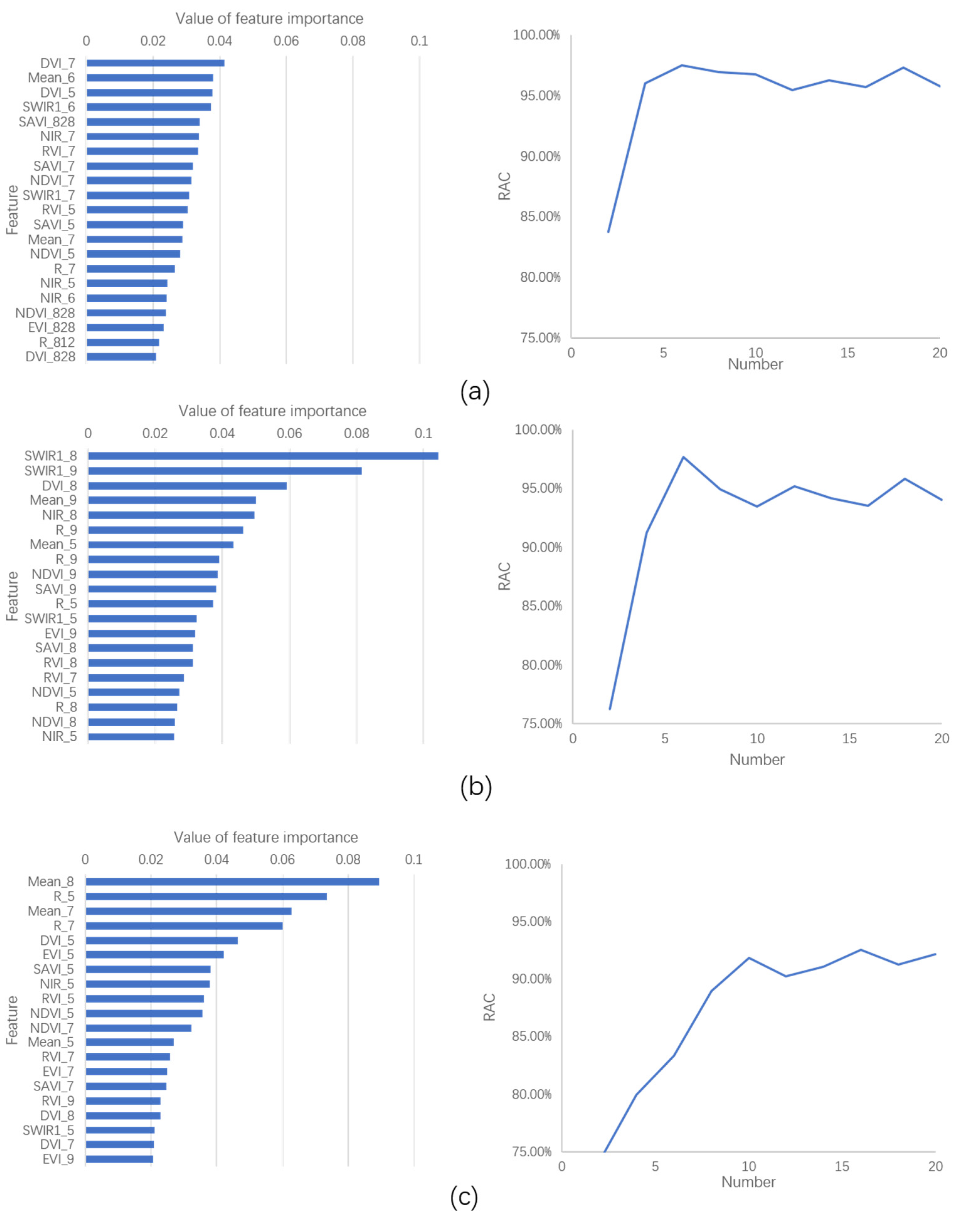
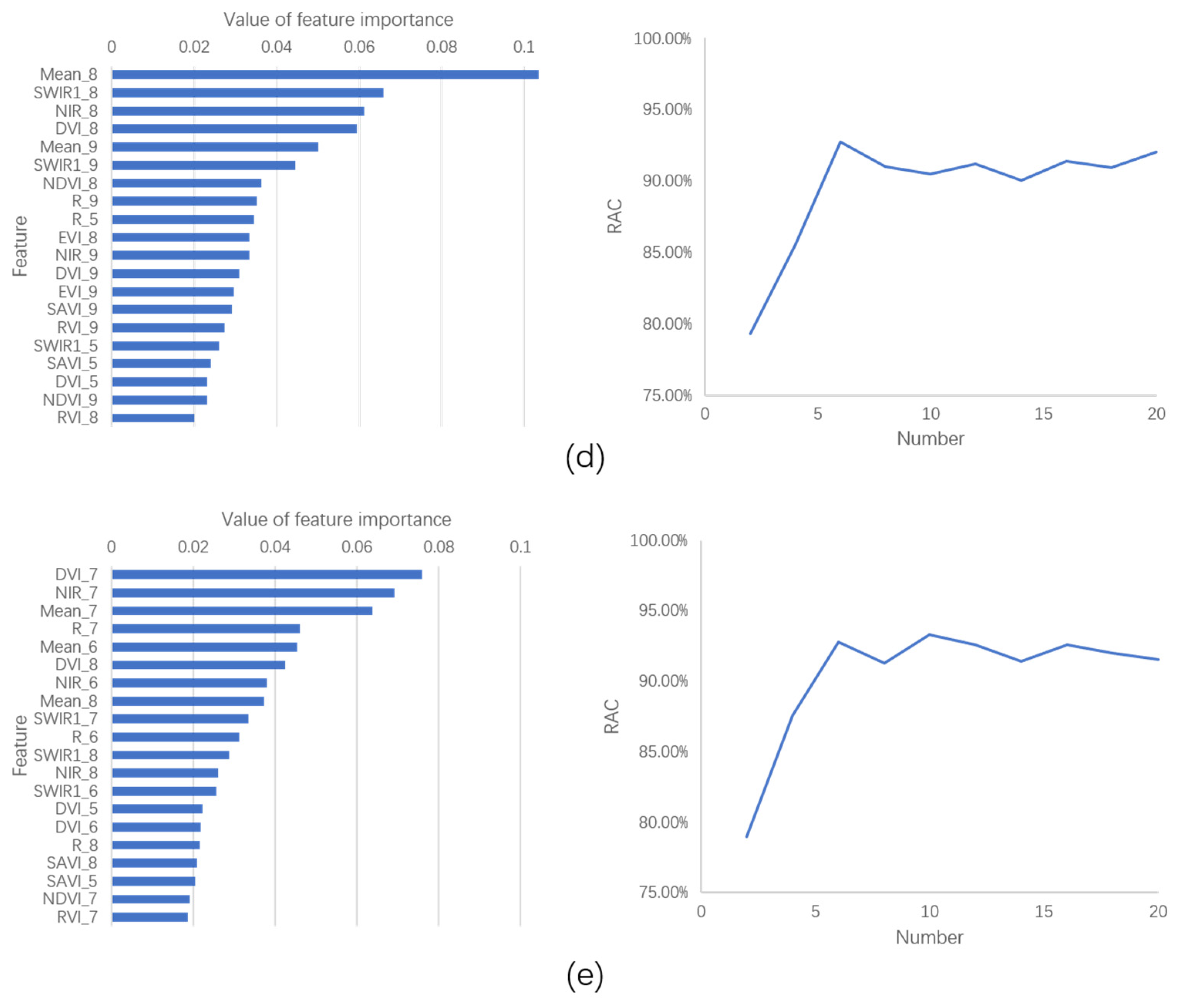
The random forest (RF) algorithm can sort the importance of each feature in the model, but it cannot determine how many features should be selected to participate in the classification to get the best result. Therefore, the problem of how to determine the number of features to participate in the classification is difficult. In this study, the RF algorithm was used to experiment with feature importance assessment in five regions: Alaer, Aksu, Wensu, Awat, and Xinhe. The ranking results are shown in Figure 5. Considering that too many features may lead to information redundancy and decreased computational efficiency, this study selected the top 20 important feature bands, tried different band combinations in a stepwise manner, and then used RF for classification. The classification results can provide a reference for determining the number of features.
According to the feature ranking results shown in Figure 5, the feature scores of each county are quite different. In Alaer city (a), the value of the most crucial feature was only 0.04, while in Aksu city (b) and Awat county (d), this value exceeded 0.1. This is related to the number of features involved in sorting. Alaer city (a) had six remote sensing images with a total of 96 features participating in the model training, while Aksu city (b) had only three remote sensing images with a total of 48 features. Because all the features were used when constructing the decision tree in RF when there were too many features, the importance score of a single feature would decrease, and the difference in the scores of each feature would become smaller. This is one of the drawbacks of the random forest algorithm for feature importance evaluation.
According to the RAC curve, when the number of features was less than six, the RAC was lower, and the curve showed a rapid upward trend. When the number of features was between 6 and 10, the RAC curve gradually stabilized. After the number of features exceeded 10, the RAC curve still fluctuated, but increasing the number would not significantly increase the RAC. Therefore, it is speculated that a maximum local value of RAC could be obtained when the number of features was between 6 and 10. Therefore, considering the classification accuracy and work efficiency, 6, 8, and 10 feature bands were selected as the three preferred combinations of features for classification.
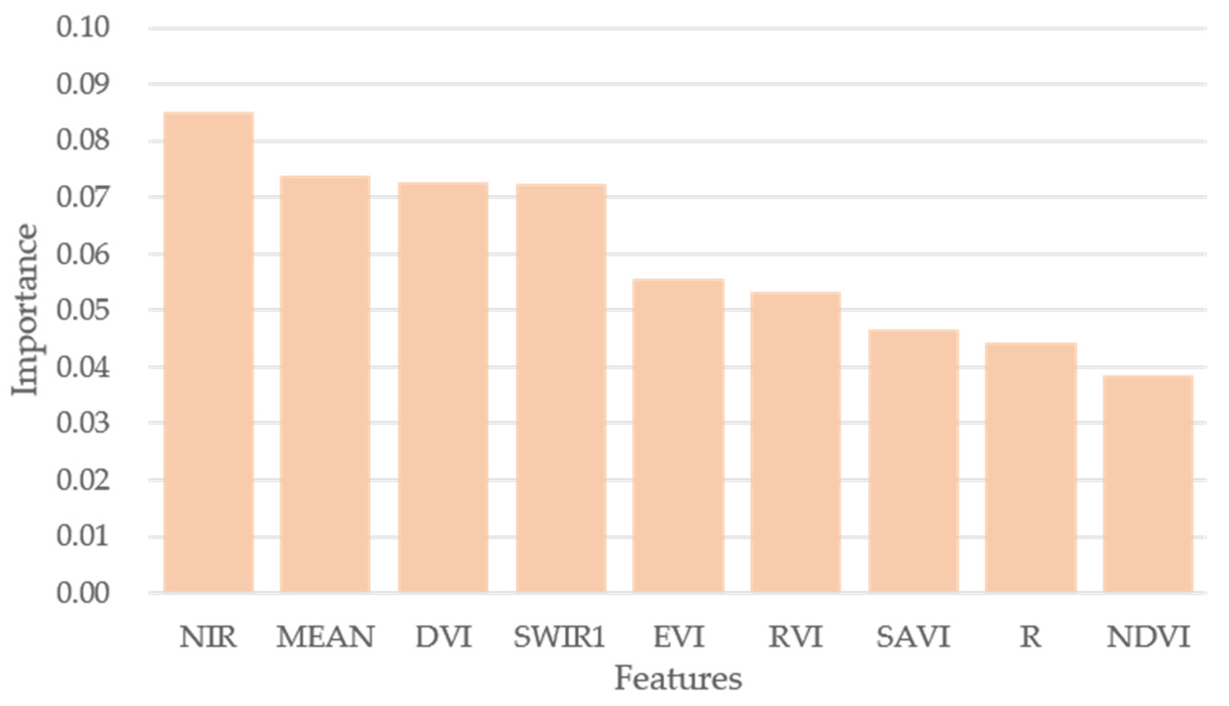
The top 20 features of 10 counties were counted and ranked by average importance, Figure 6. Firstly, the NIR band had the highest ranking of importance among all the features, indicating that it plays an essential role in improving the classification accuracy in this experiment. In addition, the SWIR1 band and the R band were also important spectral features. Secondly, the GLCM mean was ranked high in importance among the eight texture features, but other texture features were not important in the experiment. Finally, DVI had the highest score of importance among the five vegetation indices, while the other four NDVI have relatively low scores. The results showed that the RF algorithm had the potential to determine the number of classification features and rank the feature contributions.

4.2. Optimal Classification Time

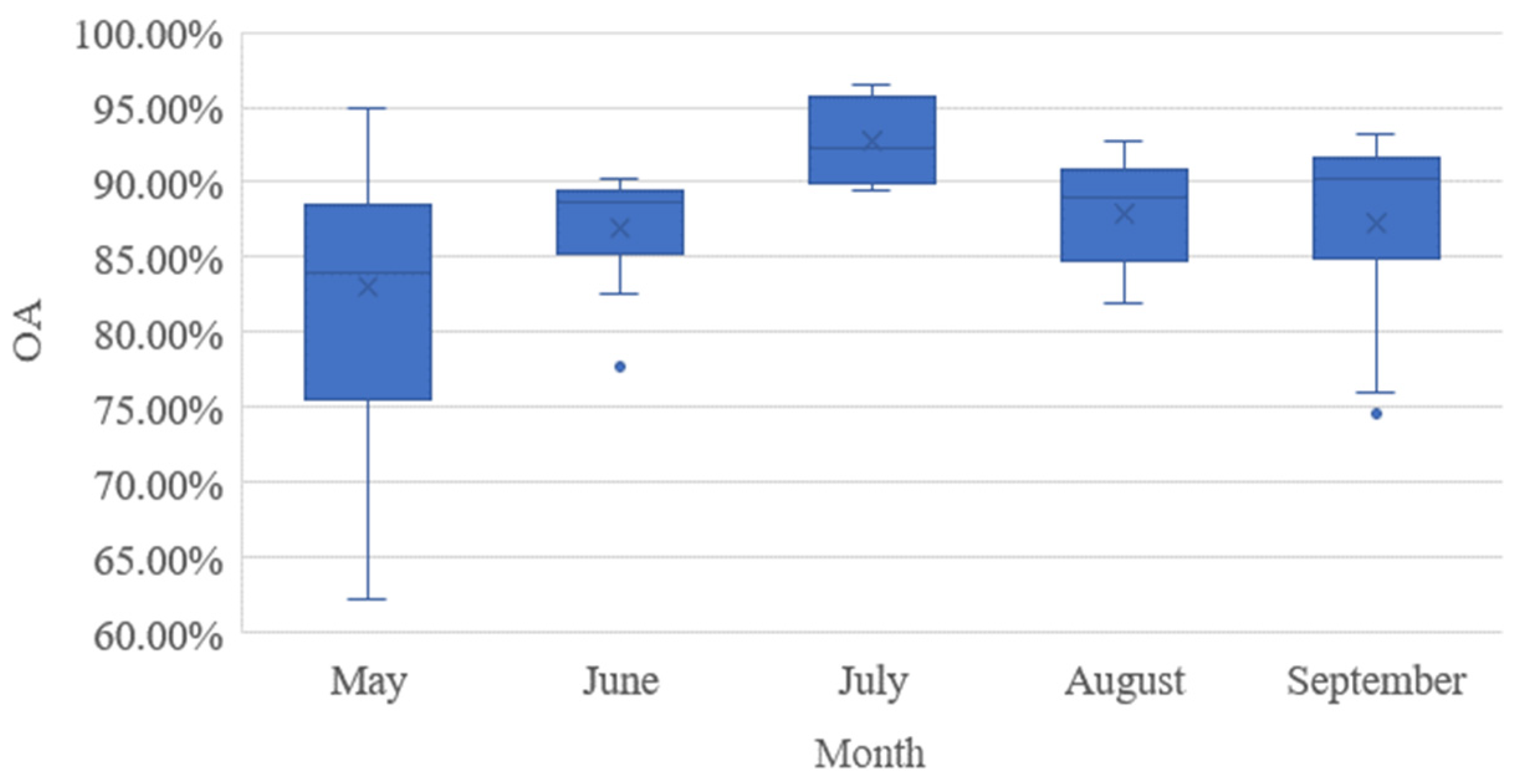
To evaluate the optimal classification time of the experiment, the overall accuracy (OA) of all single-phase images is plotted as a box plot, Figure 7. It can be seen that July had the highest average OA and the lowest degree of dispersion, which is the most suitable month for classification. In the study area, cotton is generally sown in April. When the cotton is in the flowering period in July and August, it can be easily identified on remote sensing images. The vigorous growth gives the remote sensing images little difference within the field, and they rarely produce the “salt and pepper phenomenon”. However, due to climate and other reasons, July images were heavily affected by clouds, and the number of high-quality images available was significantly lower than in other months. This means that remote sensing images at the best time may not be available, and combining multi-temporal images and multi-features is necessary to improve classification accuracy.
June and August were the other two months with good results. In May, cotton is in the early stage of growth and development, and the image is greatly affected by the soil background. In September, cotton entered the boll opening period and began to drop leaves. Due to the different harvest times between cotton fields, cotton fields at the same time may show different states, resulting in misclassification. Therefore, these two months are not suitable for cotton classification. Although there are individual classification results of these two months with high accuracy, the overall dispersion was very high, and the classification results were unstable.

4.3. Classification Results

To evaluate the impact of image data on the classification results, the classification experiments of 10 counties were divided into four groups, and each group was classified by using single time spectrum, multi-time spectrum, multi-feature image, and feature selection image, respectively. Based on three classification algorithms, SVM, ANN, and RF, the five indicators of each group of classification results were counted. Because there were too many experimental data points, only the classification results of the best method in each group of experiments are listed in Table 5.
From the best classification results of each county listed in Table 5, it can be concluded that the group based on single time spectral image classification often had the lowest classification accuracy, which indicates that the combination of multi-time image and multiple image features is helpful to improve the classification accuracy. In addition, multiple image features could achieve higher overall accuracy in most cases over using only multiple temporal, spectral images. The overall classification accuracy of the image after feature selection may be slightly lower than that of all features, but it is rarely lower than that of spectral images only. In conclusion, multi-features can usually achieve higher classification accuracy, and RF classification algorithms can usually be used as the best classifiers. After feature selection, the classification efficiency can be significantly improved.
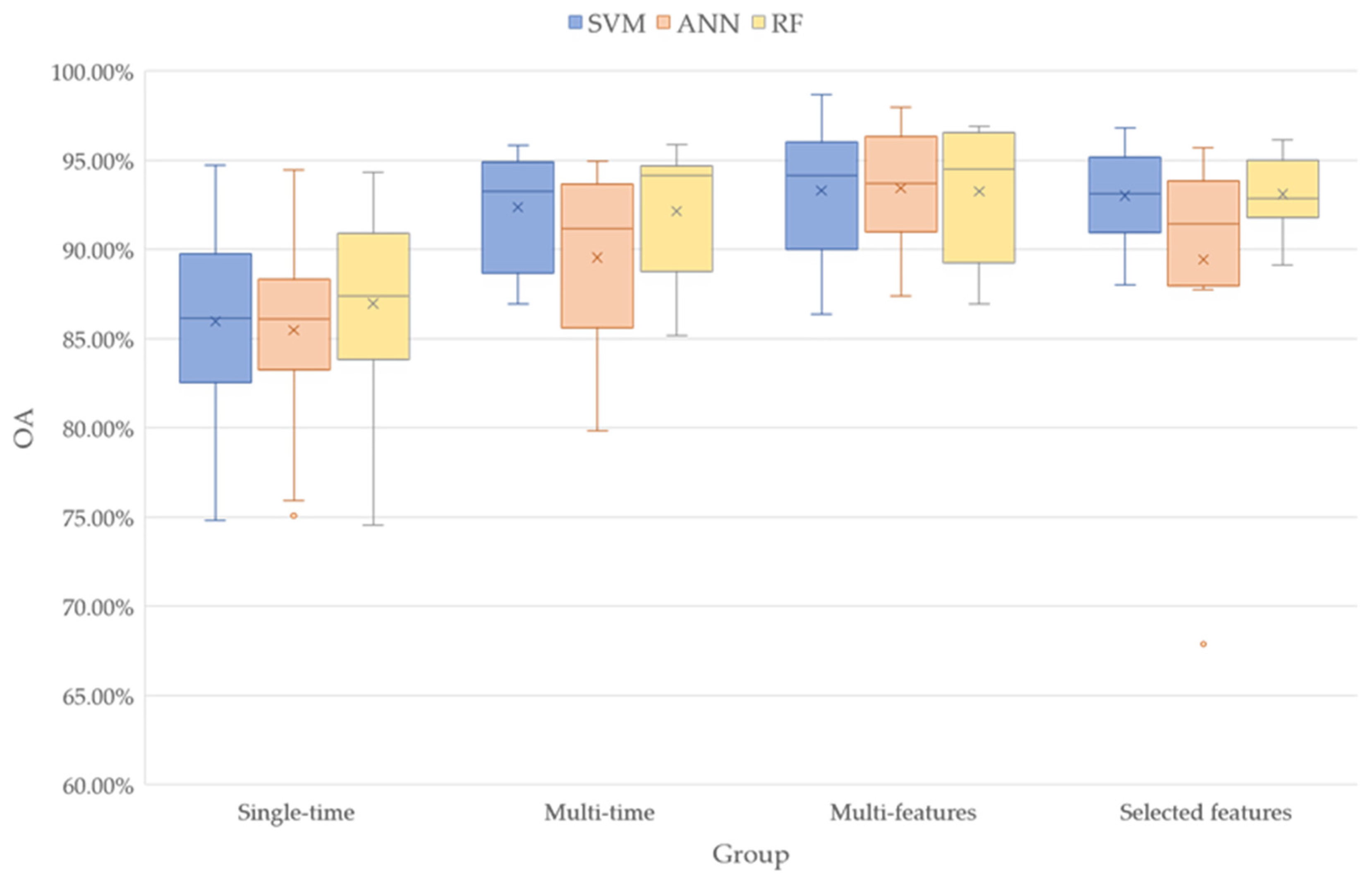
According to the three classification methods, the overall accuracy of the four groups of experimental results was plotted into a box plot, as shown in Figure 8. Results with an overall accuracy lower than 50% were not counted, and the following conclusions were drawn:
(1) Compared with the four classification results, the classification based on the single-time spectral image had the lowest average accuracy. The highest overall accuracy was found in the multi-features group, which also had the highest average accuracy, indicating that the addition of vegetation indices and texture features improved the classification accuracy. The average accuracy of the selected features group was second only to that of the multi-features group, but the data interval was more convergent (except for one discrete point). This indicates that the excessive number of features in the multi-feature group may have a negative impact on the classification results (in the data not included in Figure 8, there were five classification results in the multi-feature group that had an average accuracy of less than 50%). Feature selection eliminates these negative features and makes the classification data more reliable. The classification accuracy of the multi-time group was higher than that of the single-time group but lower than that of the other two groups. The single-time group achieved the lowest accuracy due to the inability to distinguish the phenological characteristics of crops.
The selected features group used less than 10 feature bands, and the average accuracy of all classification results in this group was 92.12%, which is 0.92% higher than the overall accuracy obtained by She et al. [44], using 29 feature bands. In Alaer’s experiment, 10 feature bands were selected from 96 feature bands using the feature selection method, the data volume was reduced by 90%, and the calculation amount was greatly reduced. The overall accuracy of the classification was only 0.19% different. On the basis of accuracy, data redundancy was avoided. Feature selection allowed us to use fewer feature bands to obtain higher classification accuracy. In another crop classification study, the overall classification accuracy using multiple feature combination methods reached 87% [45], and our average accuracy was 5.12% higher. For the cotton category, the selected features group has the best result statistics, with an average user accuracy of 91.71% and an average producer accuracy of 97.76%, indicating that the commission error of cotton is higher than the omission error and misidentifying other crops as cotton may overestimate cotton area.
(2) Comparing the performance of the three classifiers, the experimental results show that RF can get the best average overall accuracy in the single-time classification. In the classification results of the multi-features group, the average accuracy of SVM and RF was similar, but the median of RF was higher. The classification results of multi-feature groups showed that SVM achieved the maximum value, but the median was lower than RF, and the mean was similar. The classification results of RF had lower dispersion, indicating that it had better stability. There is a similar rule in the selected feature group. SVM had a higher maximum value, but was more discrete than RF, and the average accuracy of the two was approximately equal. The overall performance of ANN was worse than SVM and RF, but its performance in the multi-features group was acceptable, which may indicate that ANN is more suitable for processing higher-dimensional data. The dispersion of the classification results obtained by ANN was greater than that of RF and SVM, which was similar to the research conclusion of Raczko et al. [33]. There are too many modeling parameters of ANN, and it is difficult to determine the most suitable parameters, which may be the reason for the poor classification results. In summary, the RF classifier showed higher accuracy and stability.
Based on the above analysis, combining multiple image features for classification can effectively improve classification accuracy. Selecting image features can eliminate useless features, reduce computational expenses, and the classification accuracy will not be significantly reduced due to feature selection. SVM and RF have little difference in the performance of multi-feature image classification, but the dispersion of the classification results of RF is lower, and the training speed is higher than SVM, which is more suitable for multi-feature image classification.

4.4. Regional Applicability

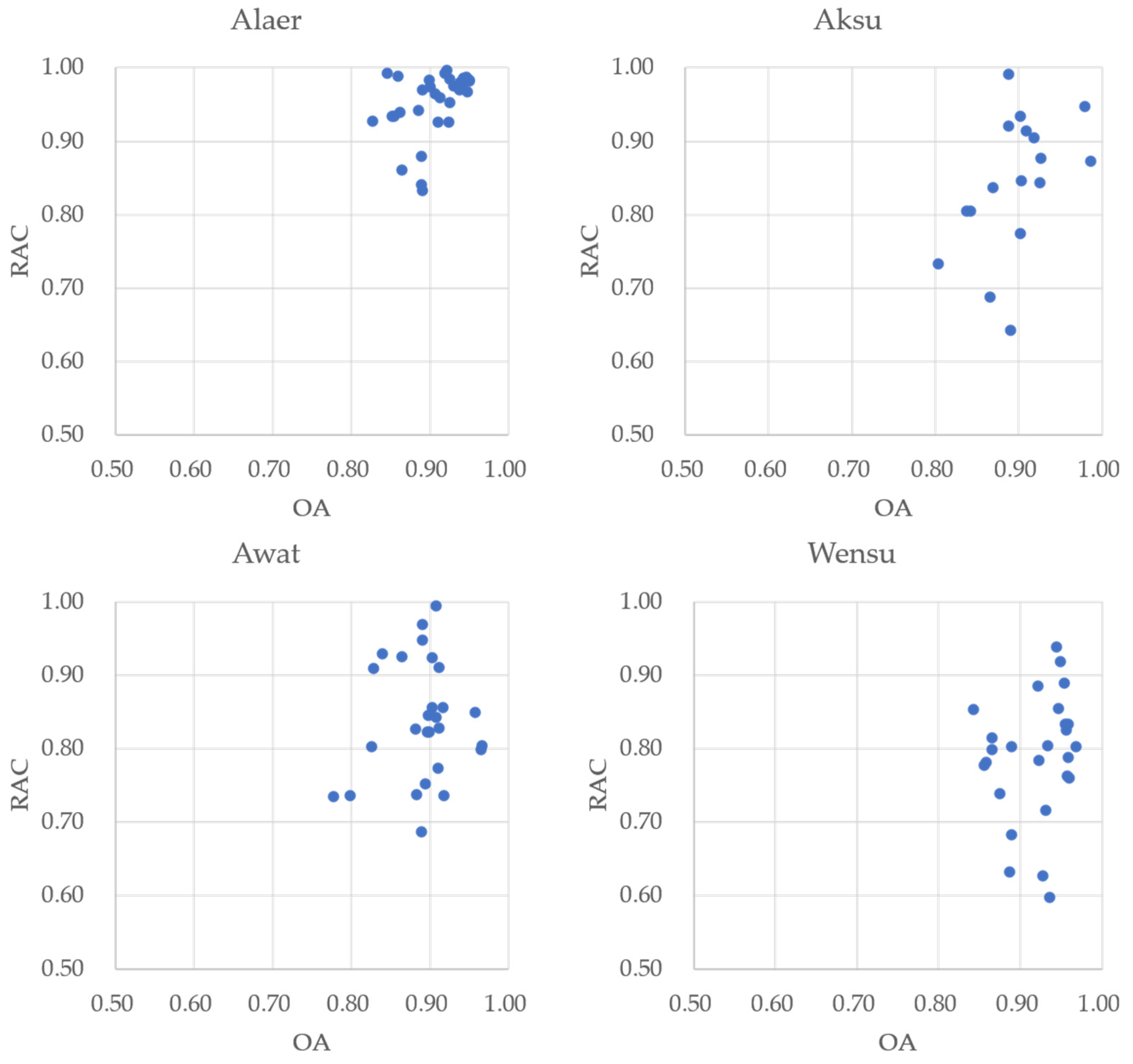
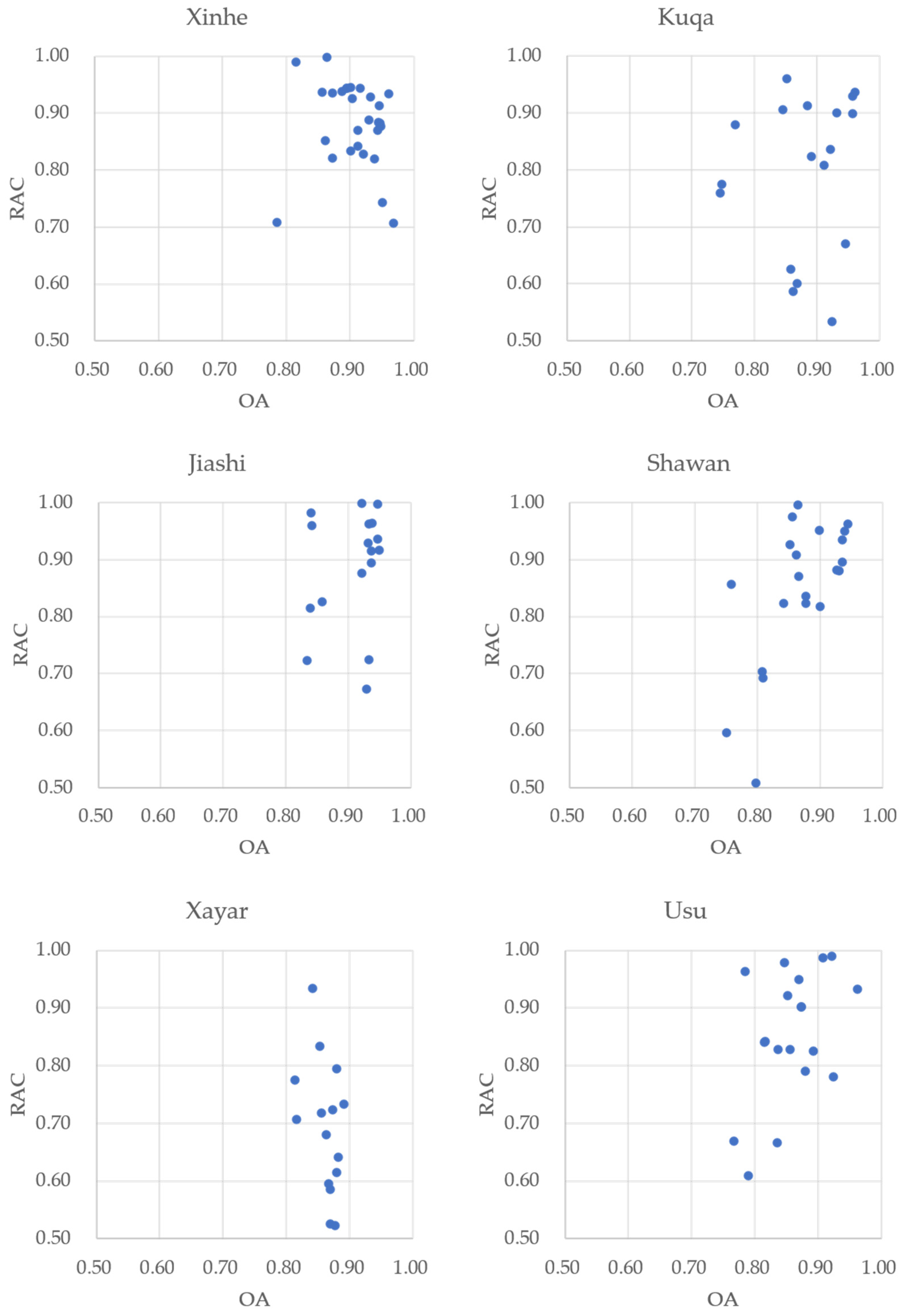
It can be seen from the previous section that the classification results of the combined multi-feature images in each county were generally better than using only the multi-spectral images, which shows that the multi-feature combined classification method can significantly improve the overall accuracy. However, there are significant differences in the classification results between regions, which is not reflected in the analysis in the previous section. Wensu County had the highest average OA, reaching 93.32%, while Aksu City only reached 88.34%. The average value of RAC in Alaer City reached 97.35%, while that in Wensu County was only 85.84%. This is related to the quality and quantity of remote sensing images in each region and related to various counties’ cropping patterns. In Figure 9, we show a scatter plot of the corresponding relationship between OA and RAC of the classification results of 10 counties to show the differences in the classification results of each region.
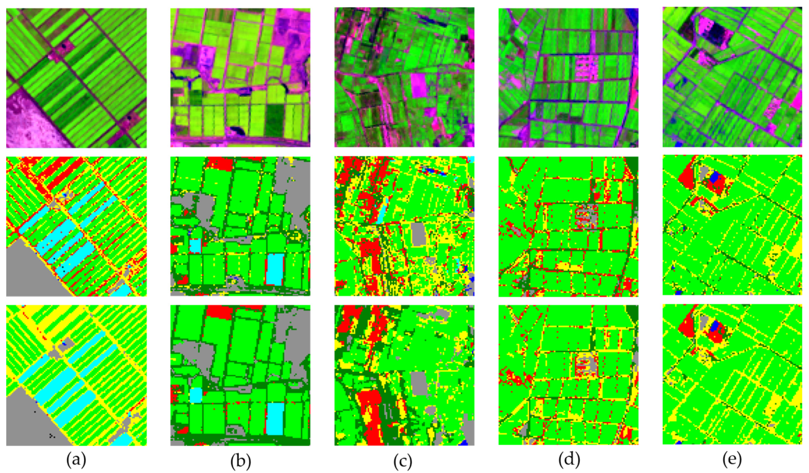
The reasons for the differences in classification between counties are as follows. Firstly, the number of remote sensing images determines the amount of information. For example, in Aksu City, only three images were available in May, August, and September, and the images were partly affected by clouds. Therefore, the classification accuracy of Aksu City was low, and the dispersion was high. In comparison, images were available every month during the cotton growing period in Alaer, and the images were clear and cloudless, so the classification results were better. Secondly, different planting patterns and crop growth conditions in each county greatly influenced the classification results. Figure 10 shows the detailed classification results of cotton growing areas in five counties. In the part of Aksu city shown in Figure 10a, due to the narrow width of the cultivated field, the mixed pixels at the edge of the field were seriously misclassified, which significantly reduced the accuracy of cotton area extraction. Even the combination of multiple features could not effectively solve this problem. In Wensu county, shown in Figure 10c, the distribution of the cultivated field was scattered, and the growth of crops in the field was different, which can easily cause misclassification, so the classification result of cotton was poor. In Alaer shown in Figure 10b, the field area was large and regular, which is beneficial to the area extraction of cotton, so the relative accuracy of cotton was better than in other areas.
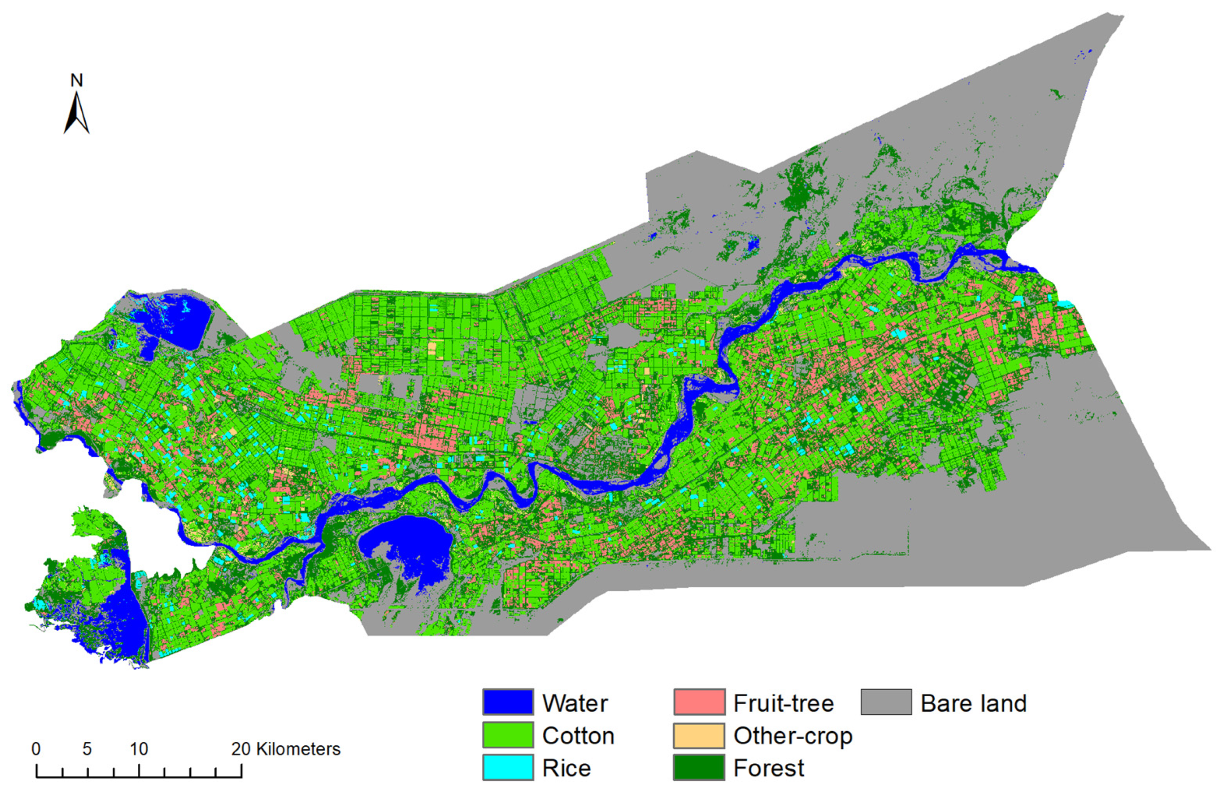
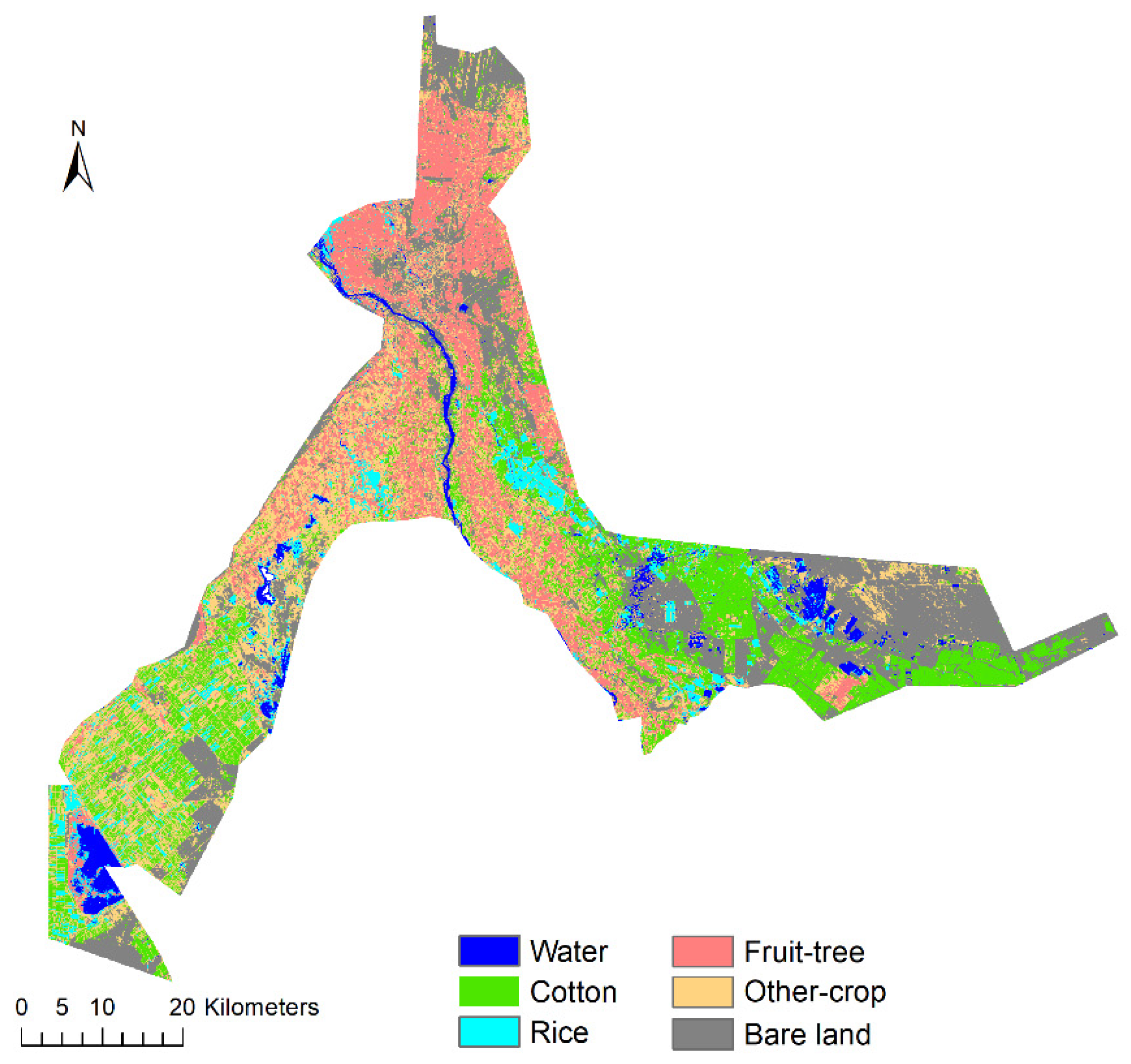
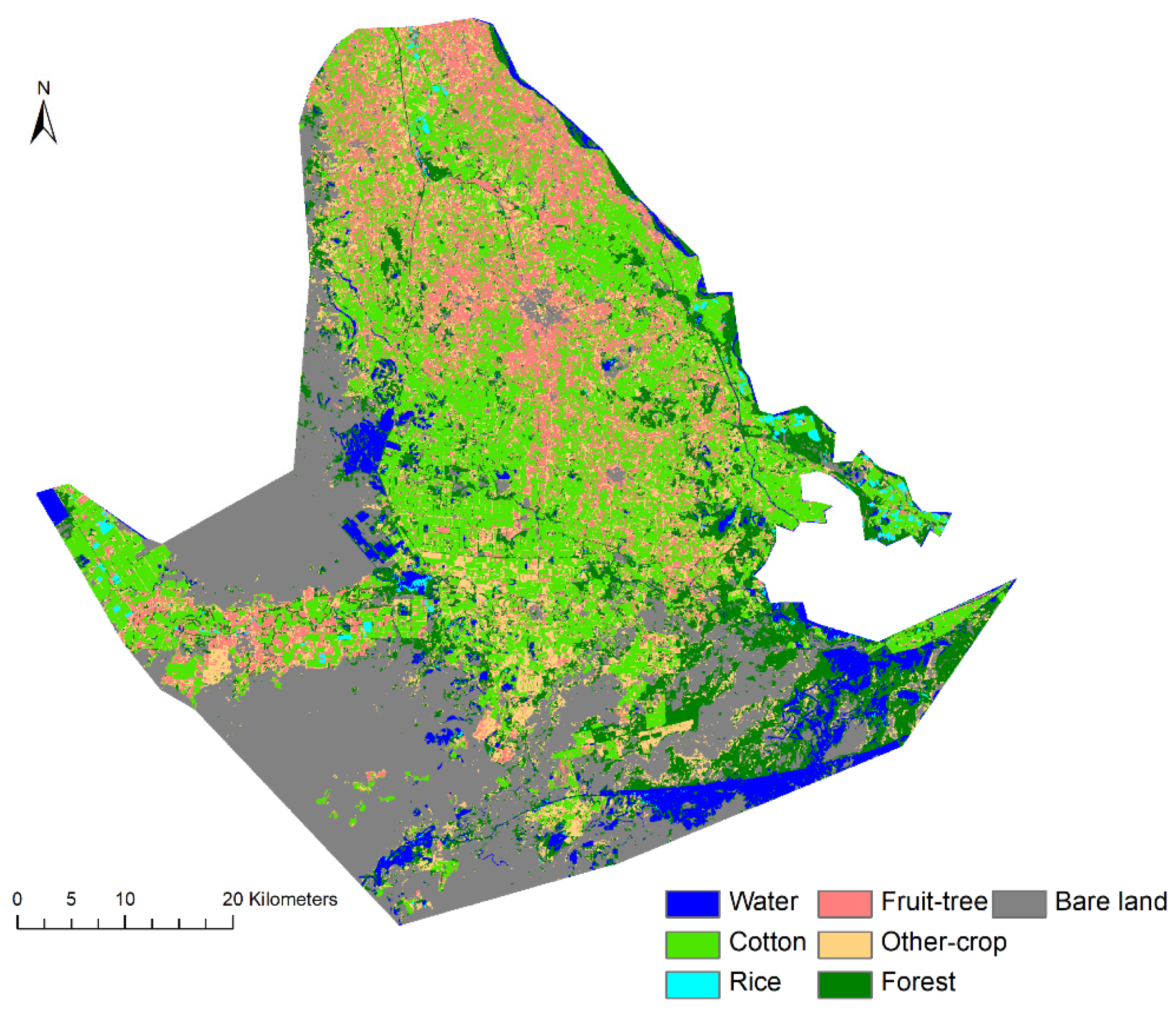
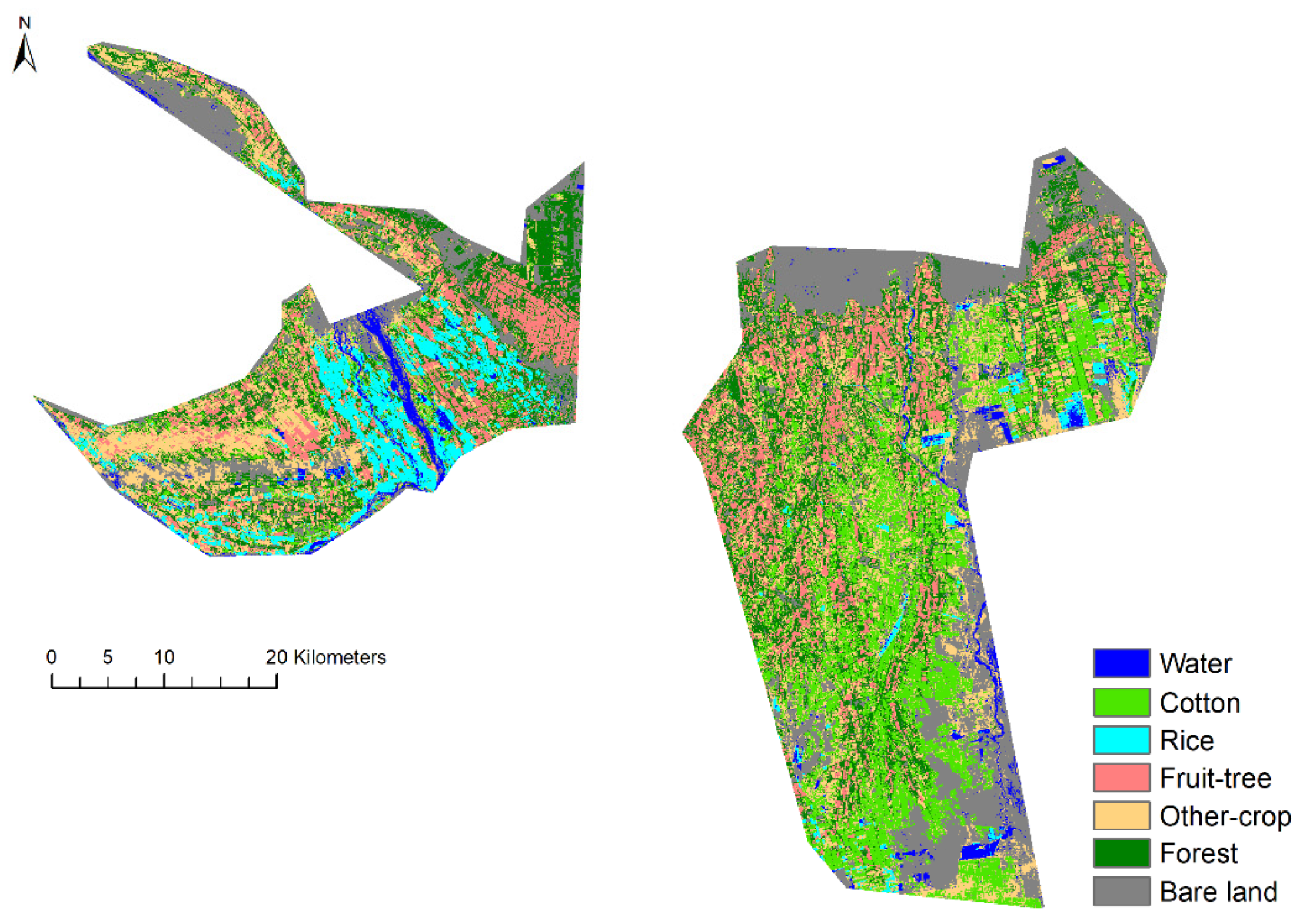
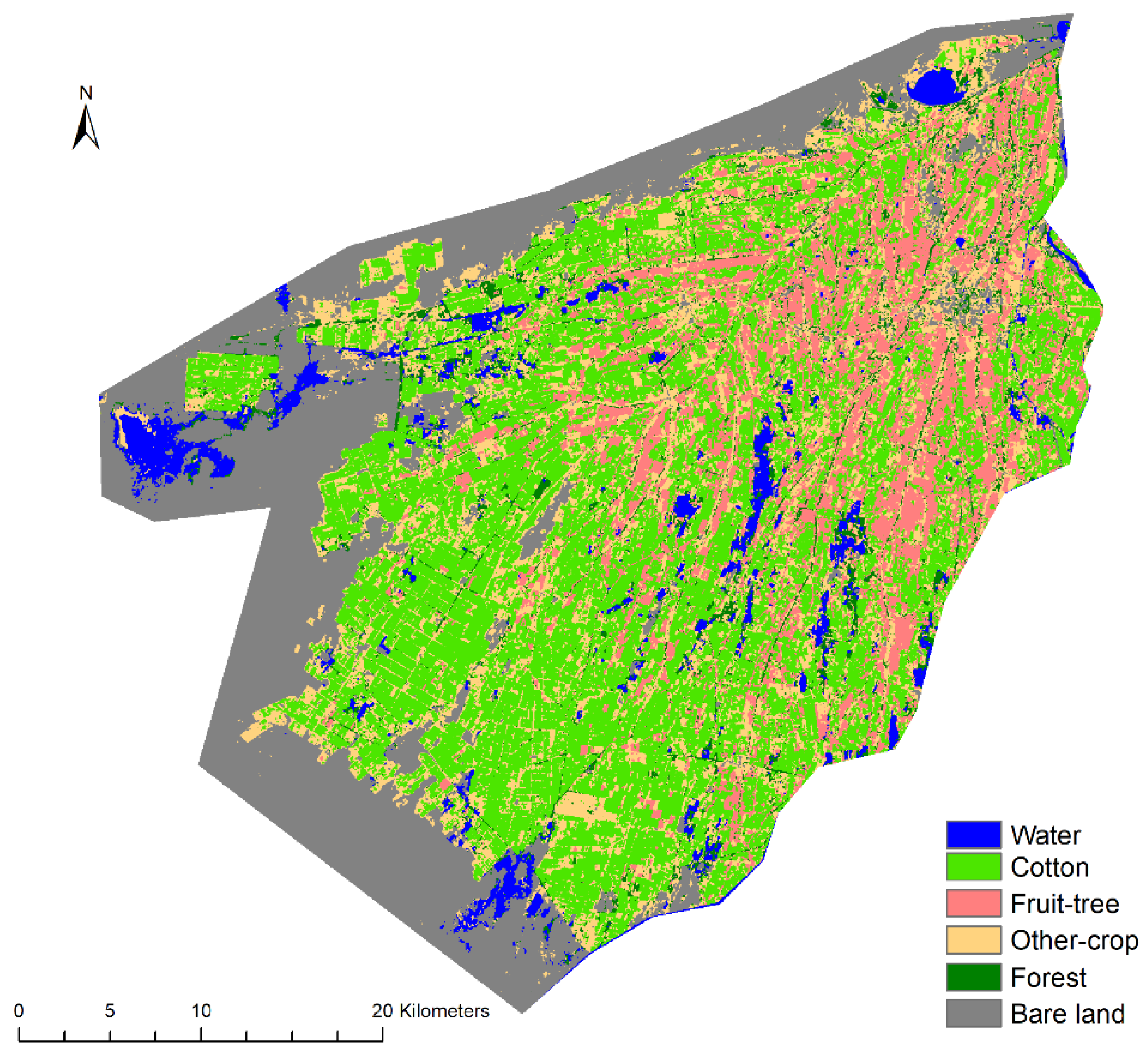
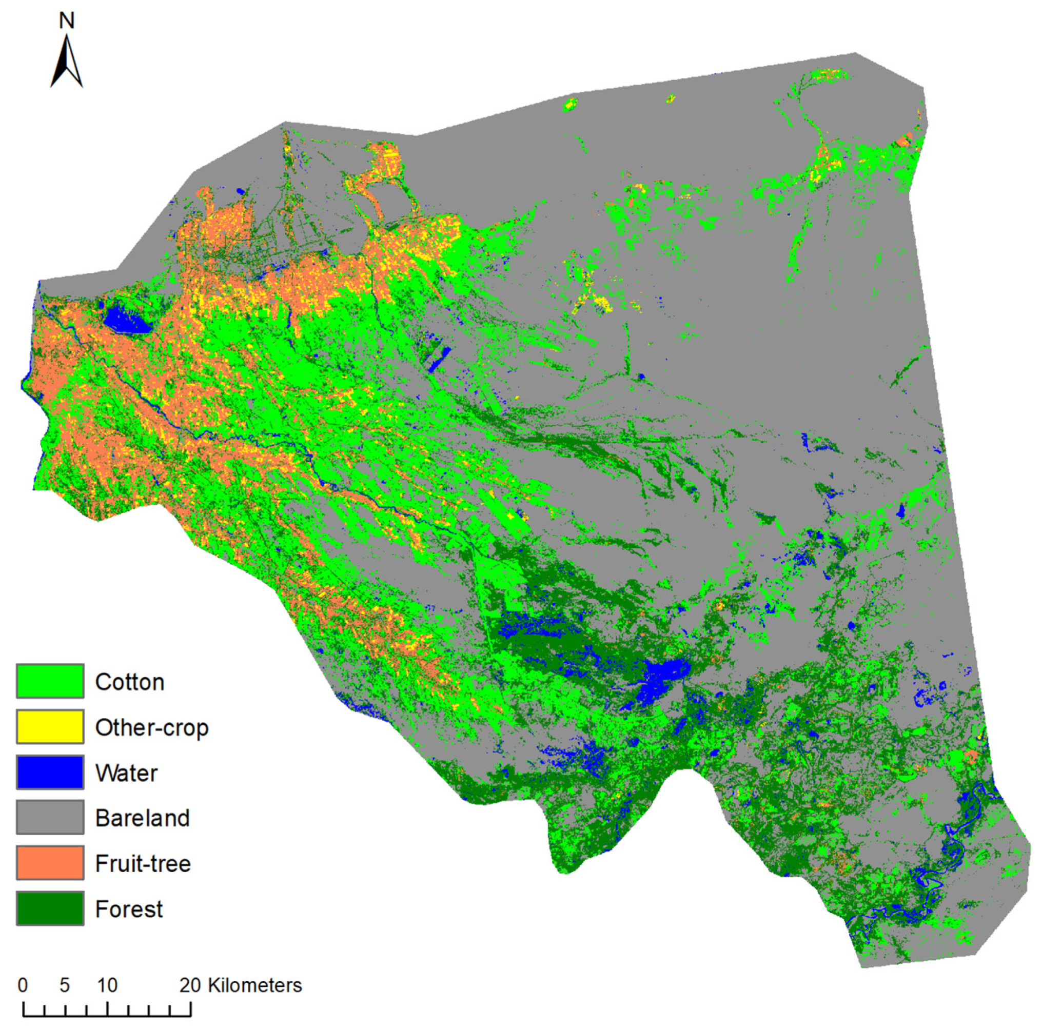
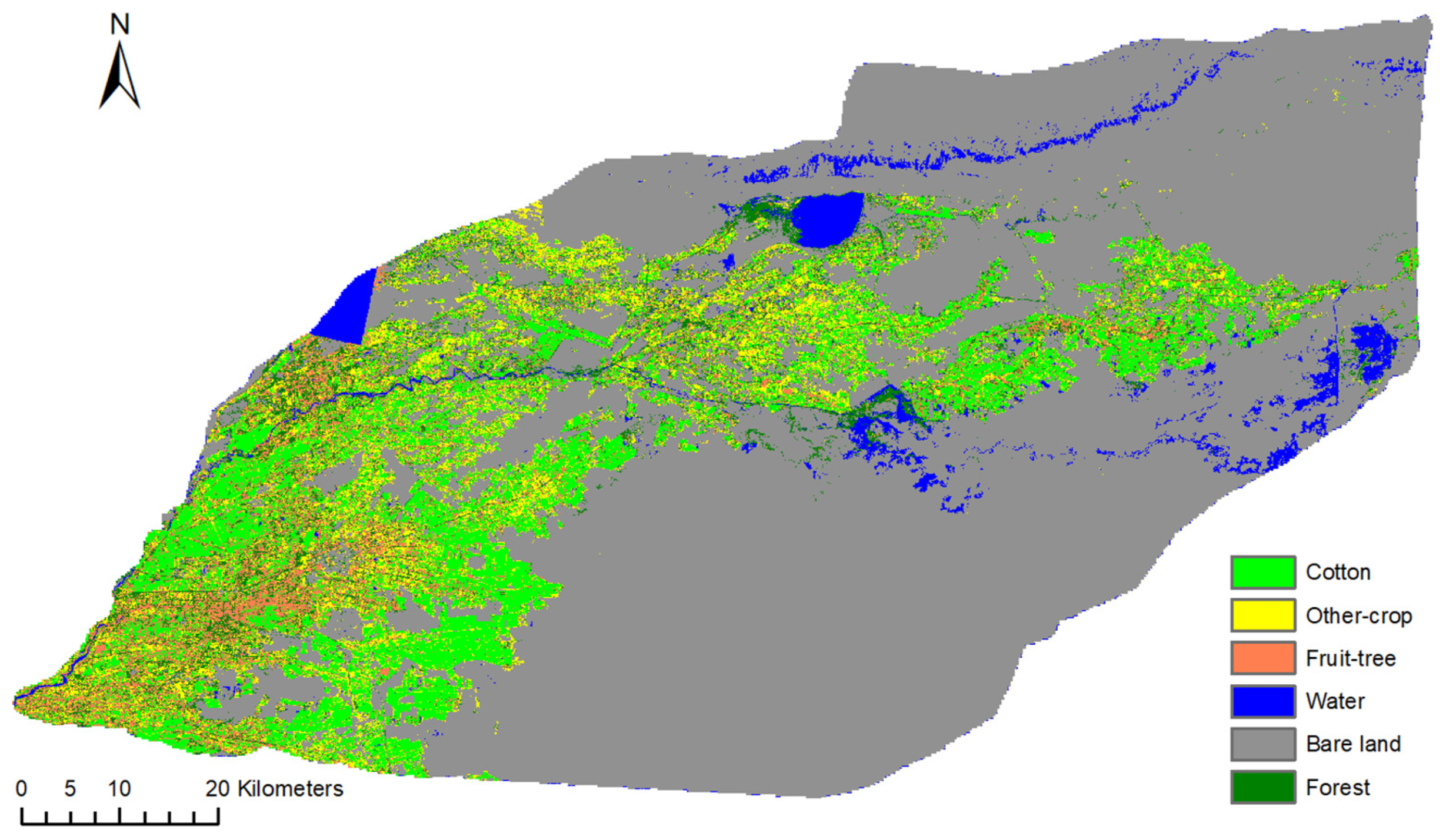
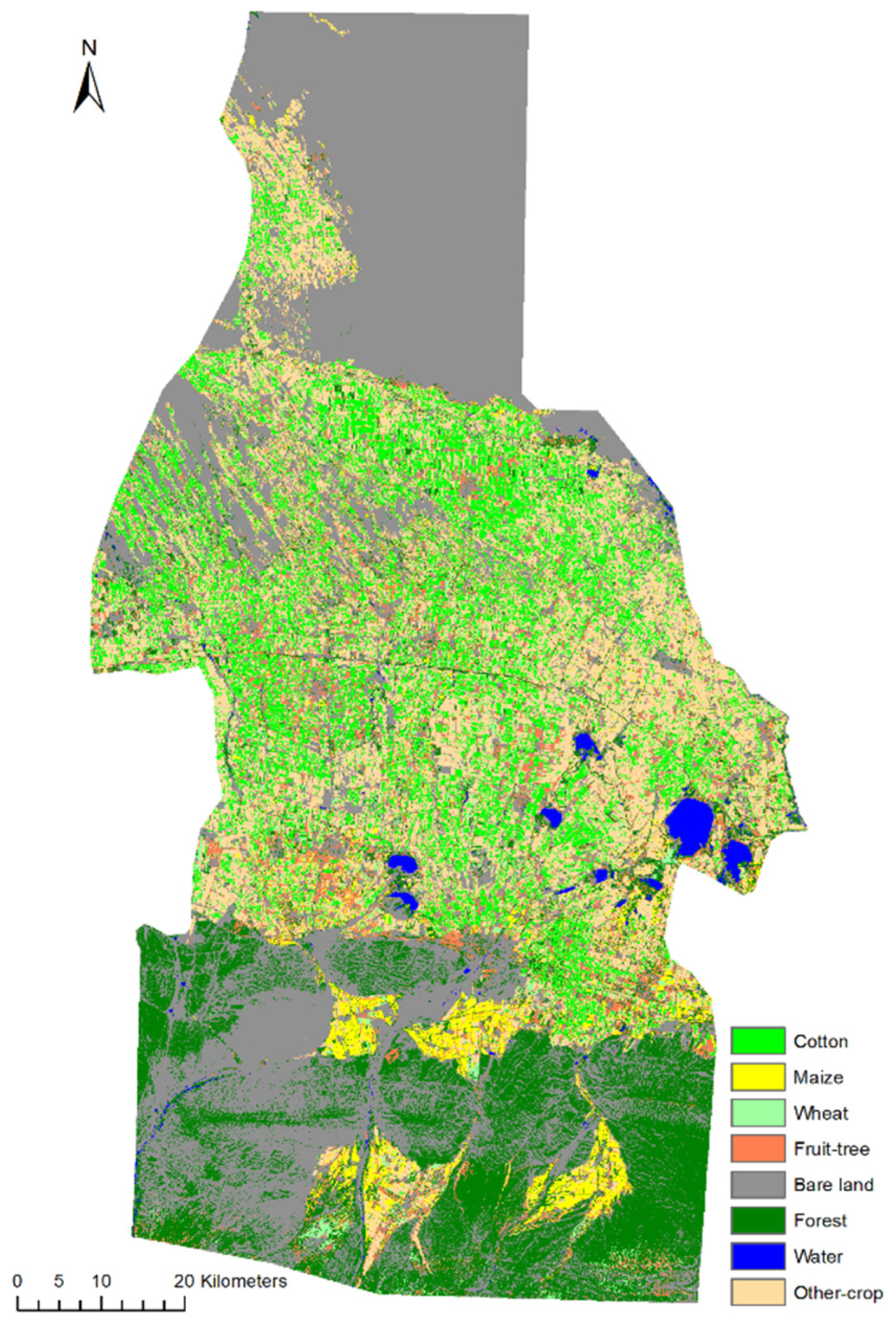
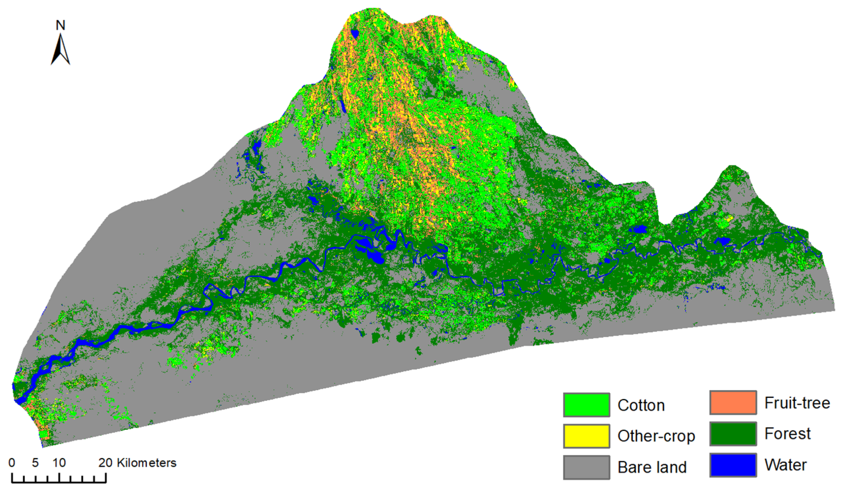
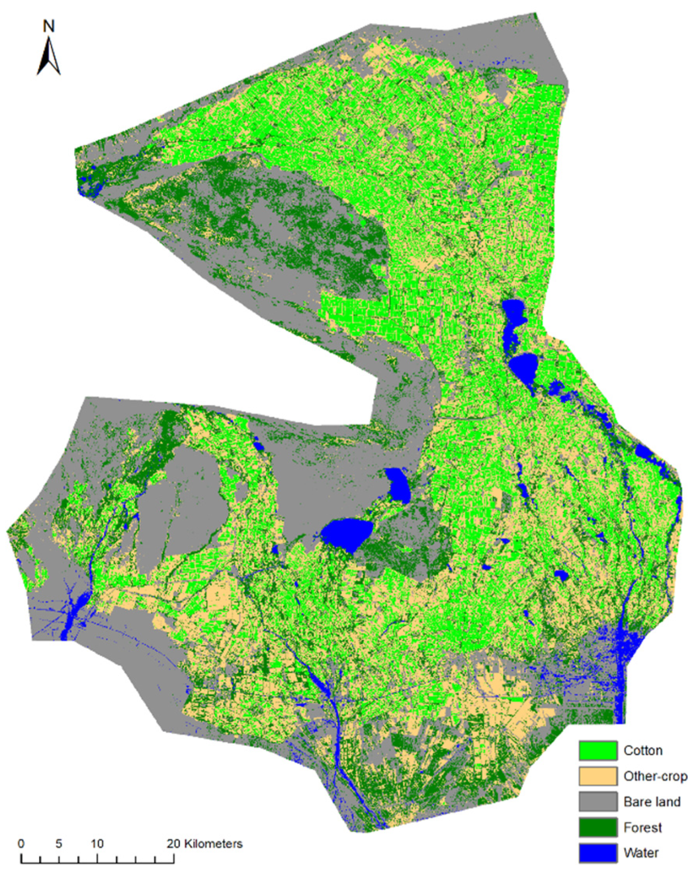
In addition, combining the local classification results of each county, it can be found that mixed pixels made more or less noise appear in all classification results due to the low image resolution. However, compared with single-phase images, the classification results of multi-feature images had greatly reduced noise and misclassification. This shows that this method can combine the characteristics of multiple features and reduce the influence of mixed pixels. To show the classification results of comprehensive multi-features more intuitively, we have listed the comprehensive multi-feature classification maps for each county, as shown in Figure 11, Figure 12, Figure 13, Figure 14, Figure 15, Figure 16, Figure 17, Figure 18, Figure 19 and Figure 20. The finally extracted cotton planting area map is shown in Figure 21.

4.5. Implications and Improvements

Previous studies have developed a series of crop classification and mapping approaches based on remote sensing images [3,4,8,12,14,18]. Many studies have focused on the acquisition period of satellite images and the performance comparison of classifiers [14,33,39,40,47]. However, in agricultural remote sensing research, the number of bands of multi-spectral imagery is limited, and the temporal and spatial resolution is low. Therefore, the phenomenon of "same spectrum with different objects" and mixed pixels often occurs, making it difficult to improve the classification accuracy. Some studies use multiple images to construct time series [20,48], which often requires complex modeling. The advantage of this research is the use of a simple feature selection algorithm to combine image spectral information, vegetation index, and texture features of different times for classification, without the need for complex modeling and analysis of a large number of features. The classification based on feature optimization can not only combine the phenological characteristics of crops in different periods, but also adds the texture features of the image so that the phenomenon of "same spectrum with different objects" and "salt and pepper noise" in traditional pixel-based remote sensing classification has been improved. The feasibility of feature selection based on the random forest algorithm was verified. It is confirmed that a lower data dimension can be used to obtain a good classification result.
This study used a random forest impurity reduction method to evaluate feature importance instead of ranking according to the number of features or the separability between classes. Although the experimental results prove that this method can provide a better feature combination, this sorting does not directly indicate the actual importance, so there may be some drawbacks of using the model method to evaluate the importance. For example, a feature band with a lot of information may be of low importance due to its strong homogeneity with other feature bands. The ranking result will be biased towards features with more categories. In addition, in terms of feature selection, this method only analyzed the influence of the number of features on the classification result, so the effect of different combinations on the separability of classes was not considered. In verifying the classification results, only the overall accuracy and the relative accuracy of the cotton area were considered, and the classification effects of other types of crops were not analyzed. These shortcomings need to be improved in future research.

5. Conclusions

This study selected ten counties as the study area and used Landsat8 OLI images available during the cotton growth period in 2017 to extract spectral features, vegetation index, and texture features from each image. The random forest algorithm was used to select these features, and three relatively mature machine learning algorithms, SVM, ANN, and RF, were used for classification. Using OA and RAC as evaluation indicators, the classification results were analyzed and compared from the three perspectives of image date, feature selection, and classifier selection. The best classification method to realize the extraction of cotton planting areas was discussed. The following conclusions were obtained:
i. Three types of features: spectral features, vegetation index, and texture features are all important in image classification. NIR shows the highest importance, and the other two spectral bands, R and SWIR1, are also essential in classification. Secondly, GLCM mean shows the highest importance in texture features, although the importance of other texture features is very low. In addition, the importance of DVI in the five vegetation indices is relatively high.
ii. July is the best time to distinguish the various vegetations in the study area, but the quality of remote sensing images during this period may be insufficient. By comparing the classification results of single-phase images and combined multi-feature images, it is confirmed that the combination of multi-features can effectively improve the classification accuracy, and this is more stable than single-phase images.
iii. The comparison of the three classifiers shows that although SVM and ANN can obtain better classification results than random forests in some cases, the RF has the best stability in multi-feature classification, and its average accuracy is almost the same as the support vector machine. In addition, the training speed of SVM and ANN is slow. Moreover, the parameters of the ANN are not easy to adjust, and only by constantly adjusting these parameters can the desired results be obtained. Combining these characteristics, random forest is efficient and straightforward and is the best classifier in this experiment.
In addition, experiments conducted in different regions show that the combined multi-feature classification method based on the RF has achieved better overall accuracy (OA) than any single temporal image. Moreover, unlike some remote sensing classification studies based on time series, this method requires only a small amount of remote sensing images, which means that its applicability is better. This research provided an effective cotton classification by comparing various methods and provided a method reference for the precise management of cotton at the county level. The conclusions obtained from the experiment can also provide references for feature selection and classifier selection in classification research.

Author Contributions

H.F. and Z.F.: co-first authors; H.F., Z.F. and C.W.: methodology and writing/preparation of the original draft. N.Z. and T.W.: validation. R.C.: investigation. T.B.: review and editing, and supervision. All authors have read and agreed to the published version of the manuscript.

Funding

This research was funded by the “National Natural Science Foundation of China (61961035), the National Key R and D Program of China (2020YFD1001005), and Bingtuan Science and Technology Program (2021DB001 and 2018CB020).

Acknowledgments

The authors would like to thank the editors and anonymous reviewers for valuable comments, which were significant in improving this manuscript.

Conflicts of Interest

The authors declare no conflict of interest.

References

  1. Shengyong, M.; Zhicai, Y. China Statistical Yearbook; China Statistics Press: Beijing, China, 2018; ISBN 978-7-5037-8587-0. [Google Scholar]
  2. Wang, X.; Huang, J.; Feng, Q.; Yin, D. Winter Wheat Yield Prediction at County Level and Uncertainty Analysis in Main Wheat-Producing Regions of China with Deep Learning Approaches. Remote Sens. 2020, 12, 1744. [Google Scholar] [CrossRef]
  3. Zhuo, W.; Huang, J.; Li, L.; Zhang, X.; Ma, H.; Gao, X.; Huang, H.; Xu, B.; Xiao, X. Assimilating Soil Moisture Retrieved from Sentinel-1 and Sentinel-2 Data into WOFOST Model to Improve Winter Wheat Yield Estimation. Remote Sens. 2019, 11, 1618. [Google Scholar] [CrossRef] [Green Version]
  4. Zhuo, W.; Fang, S.; Gao, X.; Wang, L.; Wu, D.; Fu, S.; Wu, Q.; Huang, J. Crop yield prediction using MODIS LAI, TIGGE weather forecasts and WOFOST model: A case study for winter wheat in Hebei, China during 2009–2013. Int. J. Appl. Earth Obs. 2022, 106, 102668. [Google Scholar] [CrossRef]
  5. Zhuo, W.; Huang, J.; Gao, X.; Ma, H.; Huang, H.; Su, W.; Meng, J.; Li, Y.; Chen, H.; Yin, D. Prediction of Winter Wheat Maturity Dates through Assimilating Remotely Sensed Leaf Area Index into Crop Growth Model. Remote Sens. 2020, 12, 2896. [Google Scholar] [CrossRef]
  6. Waldner, F.; Canto, G.S.; Defourny, P. Automated annual cropland mapping using knowledge-based temporal features. ISPRS J. Photogramm. Remote Sens. 2015, 110, 1–13. [Google Scholar] [CrossRef]
  7. Chakhar, A.; Ortega-Terol, D.; Hernández-López, D.; Ballesteros, R.; Ortega, J.F.; Moreno, M.A. Assessing the Accuracy of Multiple Classification Algorithms for Crop Classification Using Landsat-8 and Sentinel-2 Data. Remote Sens. 2020, 12, 1735. [Google Scholar] [CrossRef]
  8. Reddy, C.S.; Jha, C.S.; Diwakar, P.G.; Dadhwal, V.K. Nationwide classification of forest types of India using remote sensing and GIS. Environ. Monit. Assess. 2015, 187, 777. [Google Scholar] [CrossRef]
  9. Dusseux, P.; Vertes, F.; Corpetti, T.; Corgne, S.; Hubert-Moy, L. Agricultural practices in grasslands detected by spatial remote sensing. Environ. Monit. Assess. 2014, 186, 8249–8265. [Google Scholar] [CrossRef] [PubMed]
  10. Martins, V.S.; Novo, E.M.; Lyapustin, A.; Aragão, L.E.; Freitas, S.R.; Barbosa, C.C.F. Seasonal and interannual assessment of cloud cover and atmospheric constituents across the Amazon (2000–2015): Insights for remote sensing and climate analysis. ISPRS J. Photogramm. Remote Sens. 2018, 145, 309–327. [Google Scholar] [CrossRef] [Green Version]
  11. Xu, Y.; Meng, P.; Chen, J. Study on clues for gold prospecting in the Maizijing-Shulonggou area, Ningxia Hui autonomous region, China, using ALI, ASTER and WorldView-2 imagery. J. Vis. Commun. Image Represent. 2019, 60, 192–205. [Google Scholar] [CrossRef]
  12. Chen, Y.; Lu, D.; Moran, E.; Batistella, M.; Dutra, L.V.; Sanches, I.D.; da Silva, R.F.B.; Huang, J.; Luiz, A.J.B.; de Oliveira, M.A.F. Mapping croplands, cropping patterns, and crop types using MODIS time-series data. Int. J. Appl. Earth Obs. Geoinf. 2018, 69, 133–147. [Google Scholar] [CrossRef]
  13. Conrad, C.; Rahmann, M.; Machwitz, M.; Stulina, G.; Paeth, H.; Dech, S. Satellite based calculation of spatially distributed crop water requirements for cotton and wheat cultivation in Fergana Valley, Uzbekistan. Glob. Planet. Chang. 2013, 110, 88–98. [Google Scholar] [CrossRef]
  14. Conrad, C.; Fritsch, S.; Zeidler, J.; Rücker, G.; Dech, S. Per-Field Irrigated Crop Classification in Arid Central Asia Using SPOT and ASTER Data. Remote Sens. 2010, 2, 1035–1056. [Google Scholar] [CrossRef] [Green Version]
  15. Hao, P.-Y.; Tang, H.-J.; Chen, Z.-X.; Meng, Q.-Y.; Kang, Y.-P. Early-season crop type mapping using 30-m reference time series. J. Integr. Agric. 2020, 19, 1897–1911. [Google Scholar] [CrossRef]
  16. Zhang, P.; Hu, S.; Li, W.; Zhang, C. Parcel-level mapping of crops in a smallholder agricultural area: A case of central China using single-temporal VHSR imagery. Comput. Electron. Agric. 2020, 175, 105581. [Google Scholar] [CrossRef]
  17. Bagan, H.; Li, H.; Yang, Y.; Takeuchi, W.; Yamagata, Y. Sensitivity of the subspace method for land cover classification. Egypt. J. Remote Sens. Space Sci. 2018, 21, 383–389. [Google Scholar] [CrossRef]
  18. Lambert, M.-J.; Traoré, P.C.S.; Blaes, X.; Baret, P.; Defourny, P. Estimating smallholder crops production at village level from Sentinel-2 time series in Mali’s cotton belt. Remote Sens. Environ. 2018, 216, 647–657. [Google Scholar] [CrossRef]
  19. Lane, C.R.; Liu, H.; Autrey, B.C.; Anenkhonov, O.A.; Chepinoga, V.V.; Wu, Q. Improved Wetland Classification Using Eight-Band High Resolution Satellite Imagery and a Hybrid Approach. Remote Sens. 2014, 6, 12187–12216. [Google Scholar] [CrossRef] [Green Version]
  20. Gómez, C.; White, J.C.; Wulder, M.A. Optical remotely sensed time series data for land cover classification: A review. ISPRS J. Photogramm. Remote Sens. 2016, 116, 55–72. [Google Scholar] [CrossRef] [Green Version]
  21. Palacios-Orueta, A.; Huesca, M.; Whiting, M.L.; Litago, J.; Khanna, S.; Garcia, M.; Ustin, S.L. Derivation of phenological metrics by function fitting to time-series of Spectral Shape Indexes AS1 and AS2: Mapping cotton phenological stages using MODIS time series. Remote Sens. Environ. 2012, 126, 148–159. [Google Scholar] [CrossRef]
  22. Huang, J.; Tian, L.; Liang, S.; Ma, H.; Becker-Reshef, I.; Huang, Y.; Su, W.; Zhang, X.; Zhu, D.; Wu, W. Improving winter wheat yield estimation by assimilation of the leaf area index from Landsat TM and MODIS data into the WOFOST model. Agric. For. Meteorol. 2015, 204, 106–121. [Google Scholar] [CrossRef] [Green Version]
  23. Xun, L.; Zhang, J.; Cao, D.; Wang, J.; Zhang, S.; Yao, F. Mapping cotton cultivated area combining remote sensing with a fused representation-based classification algorithm. Comput. Electron. Agric. 2021, 181, 105940. [Google Scholar] [CrossRef]
  24. Domenikiotis, C.; Spiliotopoulos, M.; Tsiros, E.; Dalezios, N.R. Early cotton yield assessment by the use of the NOAA/AVHRR derived Vegetation Condition Index (VCI) in Greece. Int. J. Remote Sens. 2004, 25, 2807–2819. [Google Scholar] [CrossRef]
  25. Sun, C.; Bian, Y.; Zhou, T.; Pan, J. Using of Multi-Source and Multi-Temporal Remote Sensing Data Improves Crop-Type Mapping in the Subtropical Agriculture Region. Sensors 2019, 19, 2401. [Google Scholar] [CrossRef] [Green Version]
  26. Dong, J.; Fu, Y.; Wang, J.; Tian, H.; Fu, S.; Niu, Z.; Han, W.; Zheng, Y.; Huang, J.; Yuan, W. Early-season mapping of winter wheat in China based on Landsat and Sentinel images. Earth Syst. Sci. Data 2020, 12, 3081–3095. [Google Scholar] [CrossRef]
  27. Pelletier, C.; Webb, G.I.; Petitjean, F. Temporal Convolutional Neural Network for the Classification of Satellite Image Time Series. Remote Sens. 2019, 11, 523. [Google Scholar] [CrossRef] [Green Version]
  28. Hassan-Esfahani, L.; Torres-Rua, A.; Jensen, A.; McKee, M. Assessment of Surface Soil Moisture Using High-Resolution Multi-Spectral Imagery and Artificial Neural Networks. Remote Sens. 2015, 7, 2627–2646. [Google Scholar] [CrossRef] [Green Version]
  29. Berhane, T.M.; Lane, C.R.; Wu, Q.; Autrey, B.C.; Anenkhonov, O.A.; Chepinoga, V.V.; Liu, H. Decision-Tree, Rule-Based, and Random Forest Classification of High-Resolution Multispectral Imagery for Wetland Mapping and Inventory. Remote Sens. 2018, 10, 580. [Google Scholar] [CrossRef] [Green Version]
  30. Hubert-Moy, L.; Thibault, J.; Fabre, E.; Rozo, C.; Arvor, D.; Corpetti, T.; Rapinel, S. Mapping Grassland Frequency Using Decadal MODIS 250 m Time-Series: Towards a National Inventory of Semi-Natural Grasslands. Remote Sens. 2019, 11, 3041. [Google Scholar] [CrossRef] [Green Version]
  31. Xiong, J.; Thenkabail, P.S.; Tilton, J.C.; Gumma, M.K.; Teluguntla, P.; Oliphant, A.; Congalton, R.G.; Yadav, K.; Gorelick, N. Nominal 30-m cropland extent map of continental Africa by integrating pixel-based and object-based algorithms using Sentinel-2 and Landsat-8 data on Google Earth Engine. Remote Sens. 2017, 9, 1065. [Google Scholar] [CrossRef] [Green Version]
  32. Bazi, Y.; Melgani, F. Convolutional SVM Networks for Object Detection in UAV Imagery. IEEE Trans. Geosci. Remote Sens. 2018, 56, 3107–3118. [Google Scholar] [CrossRef]
  33. Zhu, Z.; Luo, Y.; Wei, H.; Li, Y.; Qi, G.; Mazur, N.; Li, Y.; Li, P. Atmospheric Light Estimation Based Remote Sensing Image Dehazing. Remote Sens. 2021, 13, 2432. [Google Scholar] [CrossRef]
  34. Ji, S.; Zhang, C.; Xu, A.; Shi, Y.; Duan, Y. 3D Convolutional Neural Networks for Crop Classification with Multi-Temporal Remote Sensing Images. Remote Sens. 2018, 10, 75. [Google Scholar] [CrossRef] [Green Version]
  35. Maxwell, A.E.; Warner, T.A.; Fang, F. Implementation of machine-learning classification in remote sensing: An applied review. Int. J. Remote Sens. 2018, 39, 2784–2817. [Google Scholar] [CrossRef] [Green Version]
  36. Raczko, E.; Zagajewski, B. Comparison of support vector machine, random forest and neural network classifiers for tree species classification on airborne hyperspectral APEX images. Eur. J. Remote Sens. 2017, 50, 144–154. [Google Scholar] [CrossRef] [Green Version]
  37. Thanh Noi, P.; Kappas, M. Comparison of Random Forest, k-Nearest Neighbor, and Support Vector Machine Classifiers for Land Cover Classification Using Sentinel-2 Imagery. Sensors 2017, 18, 18. [Google Scholar] [CrossRef] [Green Version]
  38. Lu, D.; Weng, Q. A survey of image classification methods and techniques for improving classification performance. Int. J. Remote Sens. 2007, 28, 823–870. [Google Scholar] [CrossRef]
  39. Al-Shammari, D.; Fuentes, I.; Whelan, B.M.; Filippi, P.; Bishop, T.F.A. Mapping of Cotton Fields Within-Season Using Phenology-Based Metrics Derived from a Time Series of Landsat Imagery. Remote Sens. 2020, 12, 3038. [Google Scholar] [CrossRef]
  40. Lebourgeois, V.; Dupuy, S.; Vintrou, É.; Ameline, M.; Butler, S.; Bégué, A. A Combined Random Forest and OBIA Classification Scheme for Mapping Smallholder Agriculture at Different Nomenclature Levels Using Multisource Data (Simulated Sentinel-2 Time Series, VHRS and DEM). Remote Sens. 2017, 9, 259. [Google Scholar] [CrossRef] [Green Version]
  41. Yuan, Q.; Shen, H.; Li, T.; Li, Z.; Li, S.; Jiang, Y.; Xu, H.; Tan, W.; Yang, Q.; Wang, J.; et al. Deep learning in environmental remote sensing: Achievements and challenges. Remote Sens. Environ. 2020, 241, 111716. [Google Scholar] [CrossRef]
  42. Chen, S.; Useya, J.; Mugiyo, H. Decision-level fusion of Sentinel-1 SAR and Landsat 8 OLI texture features for crop discrimination and classification: Case of Masvingo, Zimbabwe. Heliyon 2020, 6, e05358. [Google Scholar] [CrossRef] [PubMed]
  43. Zhang, X.M.; He, G.J.; Peng, Y.; Long, T.F. Spectral-spatial multi-feature classification of remote sensing big data based on a random forest classifier for land cover mapping. Clust. Comput. 2017, 20, 2311–2321. [Google Scholar] [CrossRef]
  44. She, X.; Fu, K.; Wang, J.; Qi, W.; Li, X.; Fu, S. Identification of Cotton Using Random Forest Based on Wide-Band Imaging Spectrometer Data of Tiangong-2. Lect. Notes Electr. Eng. 2019, 5417, 264–276. [Google Scholar] [CrossRef]
  45. You, N.; Dong, J.; Huang, J.; Du, G.; Zhang, G.; He, Y.; Yang, T.; Di, Y.; Xiao, X. The 10-m crop type maps in Northeast China during 2017–2019. Sci. Data 2021, 8, 41. [Google Scholar] [CrossRef] [PubMed]
  46. Wang, M.; Wan, Y.; Ye, Z.; Lai, X. Remote sensing image classification based on the optimal support vector machine and modified binary coded ant colony optimization algorithm. Inf. Sci. 2017, 402, 50–68. [Google Scholar] [CrossRef]
  47. Zhou, Y.; Zhang, R.; Wang, S.; Wang, F. Feature Selection Method Based on High-Resolution Remote Sensing Images and the Effect of Sensitive Features on Classification Accuracy. Sensors 2018, 18, 2013. [Google Scholar] [CrossRef] [Green Version]
  48. Chandrashekar, G.; Sahin, F. A survey on feature selection methods. Comput. Electr. Eng. 2014, 40, 16–28. [Google Scholar] [CrossRef]
  49. Cao, X.; Wei, C.; Han, J.; Jiao, L. Hyperspectral Band Selection Using Improved Classification Map. IEEE Geosci. Remote Sens. Lett. 2017, 14, 2147–2151. [Google Scholar] [CrossRef] [Green Version]
  50. Zhu, J.; Pan, Z.; Wang, H.; Huang, P.; Sun, J.; Qin, F.; Liu, Z. An Improved Multi-temporal and Multi-feature Tea Plantation Identification Method Using Sentinel-2 Imagery. Sensors 2019, 19, 2087. [Google Scholar] [CrossRef] [Green Version]
  51. Delegido, J.; Verrelst, J.; Alonso, L.; Moreno, J. Evaluation of Sentinel-2 Red-Edge Bands for Empirical Estimation of Green LAI and Chlorophyll Content. Sensors 2011, 11, 7063–7081. [Google Scholar] [CrossRef] [PubMed] [Green Version]
  52. Lin, Y.; Zhu, Z.; Guo, W.; Sun, Y.; Yang, X.; Kovalskyy, V. Continuous Monitoring of Cotton Stem Water Potential using Sentinel-2 Imagery. Remote Sens. 2020, 12, 1176. [Google Scholar] [CrossRef] [Green Version]
  53. Haralick, R.M.; Shanmugam, K.; Dinstein, I.H. Textural Features for Image Classification. IEEE Trans. Syst. Man Cybern. 1973, SMC-3, 610–621. [Google Scholar] [CrossRef] [Green Version]
  54. Zhang, X.; Cui, J.; Wang, W.; Lin, C. A Study for Texture Feature Extraction of High-Resolution Satellite Images Based on a Direction Measure and Gray Level Co-Occurrence Matrix Fusion Algorithm. Sensors 2017, 17, 1474. [Google Scholar] [CrossRef] [Green Version]
  55. Hall-Beyer, M. GLCM Texture: A Tutorial. 2017, 2. Available online: https://www.researchgate.net/publication/315776784?channel=doi&linkId=58e3e0b10f7e9bbe9c94cc90&showFulltext=true (accessed on 1 December 2021).
  56. Genuer, R.; Poggi, J.-M.; Tuleau-Malot, C. Variable selection using random forests. Pattern Recognit. Lett. 2010, 31, 2225–2236. [Google Scholar] [CrossRef] [Green Version]
  57. Rodriguez-Galiano, V.F.; Ghimire, B.; Rogan, J.; Chica-Olmo, M.; Rigol-Sanchez, J.P. An assessment of the effectiveness of a random forest classifier for land-cover classification. ISPRS J. Photogramm. Remote Sens. 2012, 67, 93–104. [Google Scholar] [CrossRef]
  58. Du, P.; Samat, A.; Waske, B.; Liu, S.; Li, Z. Random Forest and Rotation Forest for fully polarized SAR image classification using polarimetric and spatial features. ISPRS J. Photogramm. Remote Sens. 2015, 105, 38–53. [Google Scholar] [CrossRef]
  59. Li, J.; Cheng, K.; Wang, S.; Morstatter, F.; Trevino, R.P.; Tang, J.; Liu, H. Feature Selection: A Data Perspective. ACM Comput. Surv. 2017, 50, 1–45. [Google Scholar] [CrossRef]
  60. Cánovas-García, F.; Alonso-Sarría, F. Optimal Combination of Classification Algorithms and Feature Ranking Methods for Object-Based Classification of Submeter Resolution Z/I-Imaging DMC Imagery. Remote Sens. 2015, 7, 4651–4677. [Google Scholar] [CrossRef] [Green Version]
  61. Guan, H.; Li, J.; Chapman, M.; Deng, F.; Ji, Z.; Yang, X. Integration of orthoimagery and lidar data for object-based urban thematic mapping using random forests. Int. J. Remote Sens. 2013, 34, 5166–5186. [Google Scholar] [CrossRef]
  62. Congalton, R.G.; Green, K. Assessing the Accuracy of Remotely Sensed Data; CRC Press: Boca Raton, FL, USA, 2019. [Google Scholar]
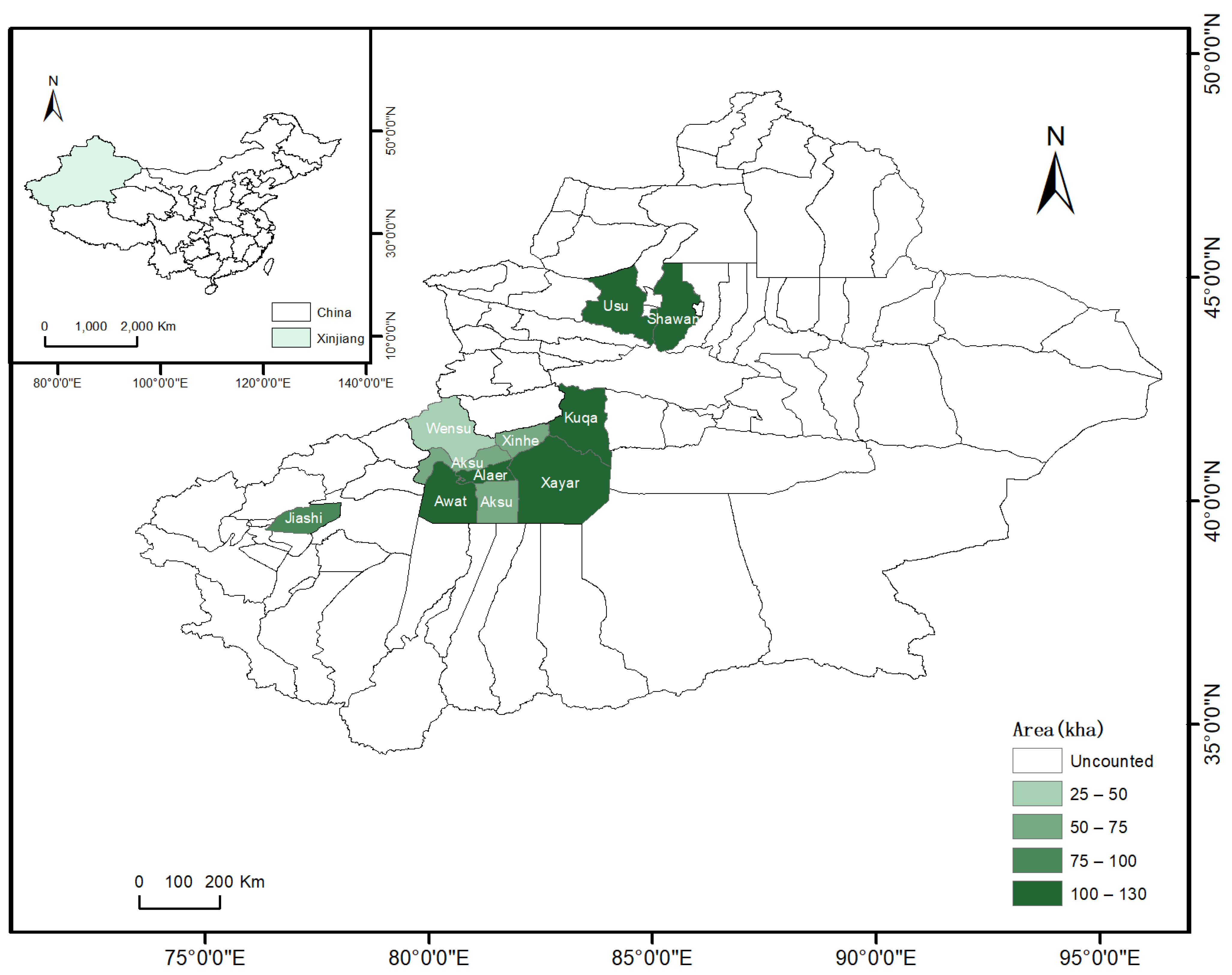
Figure 1. The geographical location of the study area and the distribution of the cotton planting area.
Remotesensing 14 00829 g001
Figure 2. The time distribution of images in various regions.
Remotesensing 14 00829 g002
Figure 3. Workflow of the cotton feature extraction and validation.
Remotesensing 14 00829 g003
Figure 4. Spectral reflectance of various ground objects in July.
Remotesensing 14 00829 g004
Figure 5. Feature ranking results of (a) Alaer City; (b) Aksu City; (c) Wensu County; (d) Awat County; (e) Xinhe County. The left side shows the top 20 feature scores of each county, the ordinate represents the abbreviation of each feature band, and the number suffixed in the feature name represents the time phase of the band. For example, DVI_7 represents the difference in vegetation index in July. The right side shows the relationship between the number of features and the RAC in each county. This result is a statistic of the results of using different numbers of features for classification.
Remotesensing 14 00829 g005aRemotesensing 14 00829 g005b
Figure 6. The average importance of various features.
Remotesensing 14 00829 g006
Figure 7. Box plot of monthly OA distribution. The box plot shows the distribution of OA for each month. The two ends of the box plot are the maximum and minimum values of the dataset, the edge of the box is two quartiles, and the middle is the median. The mark “×” gives the location of the mean value. It should be noted that the points with too large deviation in the dataset are individually marked as a discrete point but still participate in the calculation of the average.
Remotesensing 14 00829 g007
Figure 8. OA box plots of different classifiers.
Remotesensing 14 00829 g008
Figure 9. Distribution of OA and RAC in each county.
Remotesensing 14 00829 g009aRemotesensing 14 00829 g009b
Figure 10. 3 × 3 km zoom-in regions in (a) Aksu; (b) Alaer; (c) Wensu; (d) Awat; and (e) Xinhe, displaying examples of false-color composite image of best classification time with blue = band 4, green = band 5, and red = band 6 (row 1); the best single-phase classification results (row 2); and combining classification results with multiple features (row 3).
Remotesensing 14 00829 g010
Figure 11. Classification result of Alaer.
Remotesensing 14 00829 g011
Figure 12. Classification result of Aksu.
Remotesensing 14 00829 g012
Figure 13. Classification result of Awat.
Remotesensing 14 00829 g013
Figure 14. Classification result of Wensu.
Remotesensing 14 00829 g014
Figure 15. Classification result of Xinhe.
Remotesensing 14 00829 g015
Figure 16. Classification result of Kuqa.
Remotesensing 14 00829 g016
Figure 17. Classification result of Jiashi.
Remotesensing 14 00829 g017
Figure 18. Classification result of Shawan.
Remotesensing 14 00829 g018
Figure 19. Classification result of Xayar.
Remotesensing 14 00829 g019
Figure 20. Classification result of Usu.
Remotesensing 14 00829 g020
Figure 21. Cotton planting area map of 10 counties.
Remotesensing 14 00829 g021
Table 1. A summary of previous studies on cotton planted area mapping, including research areas, classification methods, and data sources at varied spatial resolutions. The classifiers used include decision tree (DT), random forest (RF), neural network (NN), and support vector machine (SVM).
AuthorStudy AreaSmallest UnitClassifierSatellite
Chen, Y.L. et al., 2018 [12]BrazilPixelsDTMODIS (250 m)
Conrad, C. et al., 2013 [13]UzbekistanObjectsDTSPOT5(2.5–5 m)/ASTER (15–30m)
Conrad, C. et al., 2010 [14]UzbekistanObjectsRFRapidEye (6.5m)/Landsat5 (30 m)
Hao, P.Y. et al., 2020 [15]ChinaPixelsNNLandsat-7/8 (30m)/Sentinel-2 (30 m)
Zhang, P. et al., 2018 [16]ChinaObjectsRF/SVMWorldView-2 (0.5 m)
Bagan, H. et al., 2018 [17]ChinaPixelsNNLandsat-5 (30 m)
Lambert, M.J. et al., 2020 [18]MaliPixelsRFSentinel-2 (30 m)
Table 2. The planting area of main crops in each unit in the study region (unit: 1000 hectares).
CottonWheatRiceMaize
Alaer100.66-4.823.23
Aksu64.9910.231.753.61
Awat101.6412.20-3.59
Wensu39.9118.848.456.39
Xinhe67.9511.34-3.27
Kuqa119.5529.25-5.71
Jiashi87.425.8-22.77
Shawan112.059.85-18.60
Xayar125.2619.00-3.25
Usu110.748.870.5415.13
Table 3. Description of Vegetation Indices.
Vegetation IndexFormulaDescription
DVI D V I = N I R R DVI is the difference in reflectivity of the two channels. It is sensitive to vegetation.
RVI R V I = N I R R RVI is the ratio of reflectance of two bands. It is suitable for areas with high vegetation coverage.
NDVI N D V I = N I R R N I R + R The range of NDVI is −1~1. It is suitable for dynamic monitoring of early and middle growth stages of vegetation
SAVI S A V I = N I R R N I R + R + L ( 1 + L ) L represents the degree of vegetation coverage, and the range is 0~1. L = 0.5
EVI E V I = N I R R N I R + C 1 × R C 2 × B + L ( 1 + L ) EVI enhances the vegetation signal by adding blue bands to correct soil background and aerosol scattering effects. In this study, L is set to 1.5, C1 is set to 6, C2 is set to 7.5.
Table 4. Calculation formulas of texture features.
Feature NameFormulation
GLCM Mean μ i = i , j = 0 N 1 i ( P i , j ) or μ i = i , j = 0 N 1 j ( P i , j )
GLCM Variance σ i 2 = i , j = 0 N 1 P i , j ( i μ i ) 2 or σ i 2 = i , j = 0 N 1 P i , j ( j μ j ) 2
Homogeneity i , j = 0 N 1 P i , j 1 + ( i j ) 2
Contrast i , j = 0 N 1 P i , j ( i j ) 2
Dissimilarity i , j = 0 N 1 P i , j | i j |
Entropy i , j = 0 N 1 P i , j ( l n P i , j )
Second Moment i , j = 0 N 1 P i , j 2
Correlation i , j = 0 N 1 P i , j [ ( i μ i ) ( j μ j ) ( σ i 2 ) ( σ j 2 ) ]
Table 5. Summary of best classification results.
GroupClassifierOAKappaUAPARAC
AlaerSingle-timeRF92.48%0.910298.30%99.63%95.22%
Multi-timeRF95.05%0.940999.74%99.63%98.28%
Multi-featuresRF95.01%0.940399.71%99.93%98.25%
Selected featuresRF94.82%0.938199.08%98.83%96.77%
AksuSingle-timeRF86.89%0.838875.83%95.83%83.70%
Multi-timeRF91.82%0.900385.44%96.93%90.43%
Multi-featuresSVM98.65%0.983297.91%98.14%87.29%
Selected featuresRF92.66%0.910284.58%96.35%87.63%
AwatSingle-timeRF91.74%0.899997.33%95.83%73.63%
Multi-timeRF89.44%0.873599.78%95.16%75.22%
Multi-featuresRF96.67%0.959699.73%95.16%80.33%
Selected featuresSVM91.21%0.893294.34%99.69%82.82%
WensuSingle-timeANN94.45%0.931897.19%99.81%93.91%
Multi-timeRF95.89%0.949594.79%100.00%83.30%
Multi-featuresSVM95.84%0.9491 95.30%100.00%78.78%
Selected featuresSVM96.79%0.960695.21%100.00%80.19%
XinheSingle-timeRF94.32%0.925794.74%98.39%86.92%
Multi-timeRF94.41%0.929994.73%99.46%88.36%
Multi-featuresRF96.88%0.959394.55%94.72%70.66%
Selected featuresRF96.13%0.949594.63%97.76%93.32%
KuqaSingle-timeSVM91.08%0.886189.70%98.91%80.82%
Multi-timeSVM95.64%0.944374.27%99.56%89.84%
Multi-featuresRF96.05%0.949680.49%100.00%93.68%
Selected featuresRF92.47%0.902268.78%94.76%83.59%
JiashiSingle-timeRF93.66%0.914982.95%98.78%89.40%
Multi-timeSVM94.66%0.928582.49%100.00%93.59%
Multi-featuresSVM93.14%0.908278.99%99.85%92.85%
Selected featuresRF94.62%0.927982.18%100.00%99.76%
ShawanSingle-timeRF89.93%86.84%100.00%99.60%95.19%
Multi-timeRF94.46%92.92%100.00%99.90%96.17%
Multi-featuresRF94.01%92.31%100.00%99.93%94.93%
Selected featuresRF93.03%91.02%100.00%98.00%88.03%
XayarSingle-timeSVM86.36%0.820992.72%99.29%67.96%
Multi-timeSVM86.96%0.8304100.00%98.35%58.53%
Multi-featuresRF88.25%0.847100.00%95.27%64.06%
Selected featuresRF89.10%0.8321100.00%93.85%73.37%
UsuSingle-timeANN97.58%0.963799.33%96.45%90.16%
Multi-timeANN96.77%0.954699.26%98.34%-
Multi-featuresSVM90.77%0.8708100.00%78.78%98.62%
Selected featuresSVM96.20%0.946698.34%98.34%93.18%
Publisher’s Note: MDPI stays neutral with regard to jurisdictional claims in published maps and institutional affiliations.